Modelling, Characterizing, and Monitoring Boreal Forest Wetland Bird Habitat with RADARSAT-2 and Landsat-8 Data

Abstract

Earth observation technologies have strong potential to help map and monitor wildlife habitats. Yellow Rail, a rare wetland obligate bird species, is a species of concern in Canada and provides an interesting case study for monitoring wetland habitat with Earth observation data. Yellow Rail has highly specific habitat requirements characterized by shallowly flooded graminoid vegetation, the availability of which varies seasonally and year-to-year. Polarimetric Synthetic Aperture Radar (SAR) in combination with optical data should, in theory, be a great resource for mapping and monitoring these habitats. This study evaluates the use of RADARSAT-2 data and Landsat-8 data to characterize, map, and monitor Yellow Rail habitat in a wetland area within the mineable oil sands region. Specifically, we investigate: (1) The relative importance of polarimetric SAR and Landsat-8 data for predicting Yellow Rail habitat; (2) characterization of wetland habitat with polarimetric SAR data; (3) yearly trends in available habitat; and (4) predictions of potentially suitable habitat across northeastern Alberta. Results show that polarimetric SAR using the Freeman–Durden decomposition and polarization ratios were the most important predictors when modeling the Yellow Rail habitat. These parameters also effectively characterize this habitat based on high congruence with existing descriptions of suitable habitat. Applying the prediction model across all wetland areas showed accurate predictions of occurrence (validated on field occurrence data), and high probability habitats were constrained to very specific wetland areas. Using the RADARSAT-2 data to monitor yearly changes to Yellow Rail habitat was inconclusive, likely due to the different image acquisition times of the 2014 and 2016 images, which may have captured seasonal, rather than inter-annual, wetland dynamics. Polarimetric SAR has proved to be very useful for capturing the specific hydrology and vegetation structure of the Yellow Rail habitat, which could be a powerful technology for monitoring and conserving wetland species habitat.

1. Introduction

The recent proliferation of Earth observation (EO) data has facilitated tremendous growth in applications of this technology. EO data have become progressively more used in species modeling, due to easy access to data almost anywhere in the world and the ability to have repeat observations of the same area, i.e., monitoring [1]. Additionally, EO data can provide continuous predictor variables which require no interpolation or sampling biases [1]. These predictor variables are often the most useful in modern presence/absence species distribution models using techniques like Boosted Regression Trees [2]. Wetland species, in particular, can benefit from habitat/species modeling with EO because these habitats are typically remote/inaccessible (boreal wetlands especially), and they are also very dynamic in both space and time. Wetland mapping and monitoring with EO sensors, such as optical, Synthetic Aperture Radar (SAR), and Light Detection and Ranging have been well studied [3,4,5,6,7], but the application of these technologies to characterize species habitat within wetlands is the next logical step which can help habitat monitoring and conservation efforts.

The species of interest for this study is the Yellow Rail (YERA–Coturnicops noveboracensis), which is an obligate wetland species that are typically very secretive. The majority of its known habitat is in the boreal forest zone [8], and it is thought to have a small and declining global population (ca. 10,000–25,000 individuals [9]). However, the species is also listed as data deficient because of the challenges associated with sampling and mapping the habitat this species requires. This led to it being listed as a species of special concern under Canada’s Species at Risk Act. Most descriptions characterize its breeding habitat as graminoid wetlands with shallow standing water, and an understory layer of senescent vegetation [10,11]. The Yellow Rail’s suitable habitat is expected to be highly specific, dynamic, and sensitive to human hydrological disturbance making it an ideal test case for EO species habitat modeling/monitoring applications.

Most previous studies using EO data to study wetlands have focused on wetland mapping and monitoring, rather than directly modeling wildlife habitat. The mapping of wetland areas versus other landcover can typically be accomplished with either optical data [12,13,14] to identify wetland vegetation or with a Digital Elevation Model to identify topographically wet areas [5,15]. The seasonal and dynamic nature of wetlands is typically captured with SAR backscatter, due to its ability to see through clouds and its strong ability to detect surface water/flooded vegetation [3]. This hybrid data approach can typically achieve very high accuracies for wetland, wetland class, and landcover maps [5,7,16], but, in the end, this categorical data may not be very useful for characterizing meaningful habitat for wetland species. Using these EO sources directly to model the species’ habitat may be a better method [16]. This method can directly correlate a species’ habitat to EO data without the intermediate step of running a species model on top of the landcover classification models, which may compound errors. These categorical landcover classifications are often not updated regularly, making species monitoring difficult when using such approaches [1]. Further, EO data can be specifically chosen to detect habitat features of interest to a given species. In the case of YERA, we would want EO data to detect and monitor the changing hydrology and capture the specific vegetation structure rather than a coarser wetland type designation.

SAR, and specifically polarimetric SAR, including both fully polarimetric and compact polarimetric configurations, have shown a strong ability to detect water/vegetation interactions and characterize wetland vegetation structure [17,18]. Certain decompositions from SAR, such as the Freeman–Durden decomposition [19], can separate SAR backscatter into useful parameters for characterizing wetland habitat: Double bounce–typically associated with flooded vegetation in wetlands; volume scattering–higher values associated with higher biomass, and rough surface–rougher surface at the scale of the wavelength. Moderate-resolution optical data should also theoretically detect graminoid vegetation, but may be limited for characterizing vegetation/water interactions. A DEM may not be of interest for YERA modeling as DEMs are typically used to distinguish wetland from upland areas, and we would expect habitat to only occur in flat wetland areas.

While species habitat modeling with EO is less common than landcover mapping with EO, there have been numerous studies that use EO for species conservation purposes. Prior studies have used optical data for species distribution models of the bird’s breeding habitat [20,21,22] or used SAR/LiDAR to model specific habitat vegetation structures for bird species [23,24]. Other studies have used SAR to map and monitor Panda habitat [25], and to characterize wetland habitat in the Brazilian Pantanal [26]. Similar polarimetric SAR and bird habitat studies have been done with Black Tern habitat in the Great Lakes region [27]. In a related study to ours, [16] used Sentinel-1, Sentinel-2 (multi-spectral optical), and DEM data to predict YERA species abundance. Species habitat monitoring is potentially a very powerful and under-utilized application of this technology, especially when monitoring dynamic habitats.

This study aims to build on the work from [16,28] by investigating the importance of polarimetric SAR from RADARSAT-2 for developing more accurate predictive models of the YERA habitat. We also investigate yearly and seasonal habitat dynamics with RADARSAT-2 and Landsat-8 data to determine if we can track changes in habitat suitability in time. The objectives of this study are divided into four parts: (1) Investigate the relative importance of polarimetric SAR for predicting YERA wetland habitat, (2) characterize YERA habitat based on the EO variables (3) explore the ability of EO data to detect changes in YERA habitat year-to-year, and (4) assess the ability of polarimetric SAR and optical data to predict suitable YERA habitat across larger areas.

2. Materials and Methods

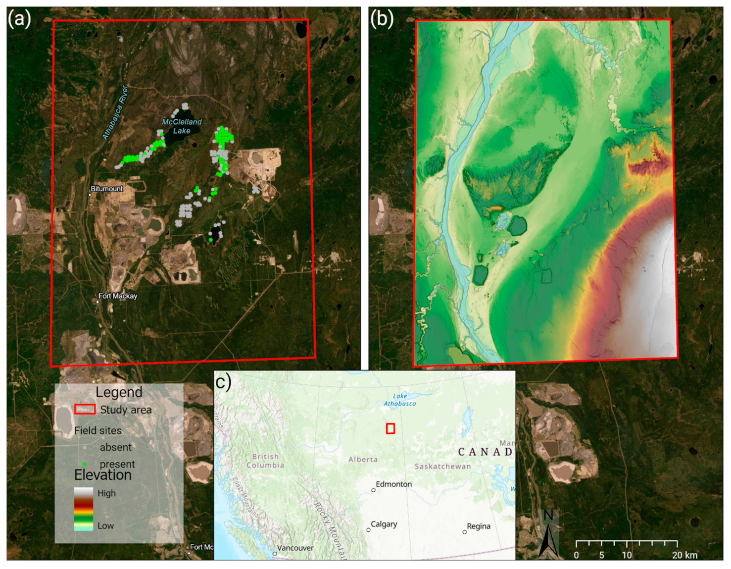
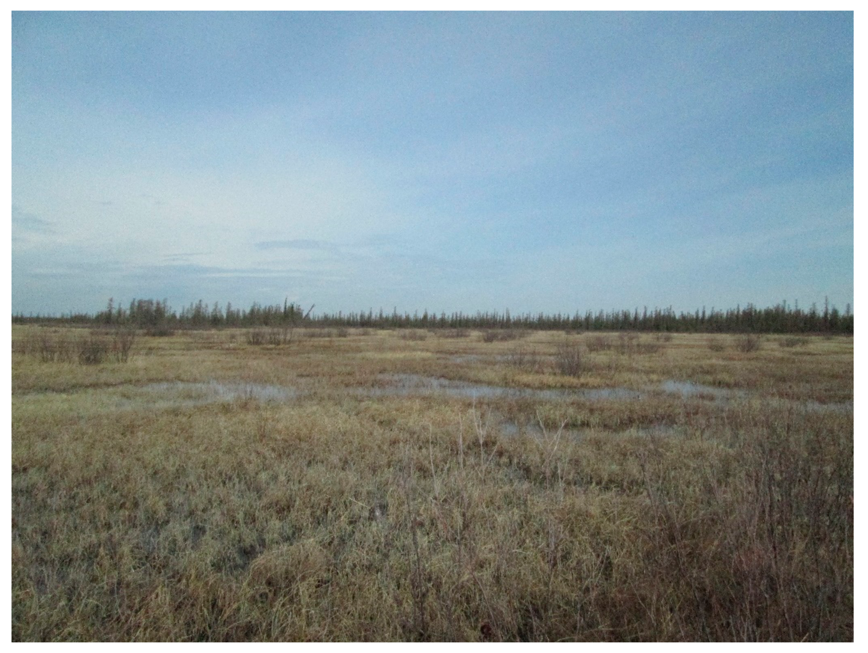
2.1. Study Area

The area of interest for this study is a 3480 km² region in northeastern Alberta, Canada (Figure 1). This is in the Boreal Plains Ecozone/Boreal Forest Natural Region, and elevation in this area is relatively flat from 200–600 m above sea level. Vegetation in this area is mainly conifer, mixed and deciduous forests, along with large peatland complexes in low-lying areas [29]. As seen in panel (a) of Figure 1, the study area is the main mining area in the Athabasca oil sands mineable area. The area has numerous open mines with associated tailing ponds and resource roads. The current extent of wetlands in the area is located around the blue field points seen in Figure 1. According to DeLancey, Simms, Mahdianpari, Brisco, Mahoney and Kariyeva [7], 30% of the study area is wetland habitat, with most of this being treed, shrub, and graminoid fens.

2.2. Yellow Rail Abundance Data

The YERA abundance data comes from previous studies in [17,29]. This data comes from autonomous recording units during field campaigns in 2013–2019. There were 203 recording units placed within wetland sites in the study area. The presence/absence of YERA at each site was determined using automated processing and human interpretation. First, a recognizer was used to filter out potential YERA calls, then, a human interpreter would validate this call. Prior work has shown that the effective detection radius for these recording units is about 250 m [30], and therefore, these sites were buffered by 250 m. These sites were then clipped to include only wetland areas using the ABMI Wetland Inventory [7], which has been suggested as best practice in Thuiller, et al. [31].

2.3. Earth Observation Data

This study used RADARSAT-2 and Landsat-8 data from 2014 and 2016 listed in

Table 1. List of images used for the analysis of the Yellow Rail habitat. Two RADARSAT-2 images were used for the 28 June 2016 date.

Satellite	Date	Resolution (m)	Data Type
RADARSAT-2	06 Aug 2014	8	Fine Quad-Pol
RADARSAT-2	28 June 2016	8	Fine Quad-Pol
Landsat-8	02 Aug 2014	30	Surface reflectance
Landsat-8	29 June 2016	30	Surface reflectance

. RADARSAT-2 Fine Quad-Pol data was provided by the Canadian Centre for Mapping and Earth Observation. The 2016 data consisted of two ascending orbit images, while the 2014 data was one ascending orbit image. The images were processed in PCI Geomatica with the following steps: 9 × 9 boxcar filter, matrix symmetrization, Freeman–Durden decomposition [19], and finally ortho-rectification and terrain correction using the ALOS digital elevation model. Parameters extracted from this data for YERA habitat modeling were the three components of the Freeman–Durden decomposition (volume scattering, double bounce, and rough surface; see [17] for a more detailed physical description of these parameters), Vertical-Vertical (VV), Horizontal-Horizontal (HH), and Horizontal-Vertical (HV) backscatter, cross-pol ratio (HH/VV), and co-pol ratio (HH/HV) (see

Table 2. List of EO inputs for Yellow Rail modeling.

Variable	Satellite	Description
HH	RADARSAT-2	Horizontal-Horizontal backscatter
HV	RADARSAT-2	Horizontal-Vertical backscatter
VV	RADARSAT-2	Vertical-Vertical backscatter
CrossPolRatio	RADARSAT-2	HH/VV
CoPolRatio	RADARSAT-2	HH/HV
DoubleBounce_FD	RADARSAT-2	Double bounce component of the Freeman–Durden decomposition
RoughSurface_FD	RADARSAT-2	Rough surface component of the Freeman–Durden decomposition
VolumeScattering_FD	RADARSAT-2	Volume scattering component of the Freeman–Durden decomposition
B2–7_	Landsat-8	Bands 2–7 from Landsat 8
NBR_	Landsat-8	$\mathrm{Normalized}\mathrm{Burn}\mathrm{Ratio} \frac{\left(B5-B7\right)}{\left(B5+B7\right)}$
NDVI_	Landsat-8	$\mathrm{Normalized}\mathrm{Difference}\mathrm{Vegetation}\mathrm{Index}\frac{\left(B5-B4\right)}{\left(B5+B4\right)}$
NDWI_	Landsat-8	$\mathrm{Normalized}\mathrm{Difference}\mathrm{Water}\mathrm{Index}\frac{\left(B5-B6\right)}{\left(B5+B6\right)}$

). The Freeman–Durden decomposition is a technique that uses the phase and amplitude part of the SAR wave to analyze the scattering characteristics of polarimetric SAR data. The volume scattering component typically represents random scattering of the SAR wave off targets like tree canopies, double bounce represents a SAR wave which bounces off two reflectors and back to the sensor (like water then vegetation), and rough surface represents scattering off of rough surfaces at the scale of the wavelength. The other parameters used from SAR are the amplitude of the SAR return in different send and receive configurations (HH, HV, VV) or ratios between their parameters (cross-pol ratio = HH/VV).

Landsat-8surface reflectance data were acquired and processed in Google Earth Engine [32]. Cloud free Landsat-8 images were chosen as close to the RADARSAT-2 dates as possible (see Table 1). From the Landsat-8 images, the Normalized Difference Vegetation Index (NDVI), Normalized Difference Water Index (NDWI), and Normalized Burn Ratio (NBR) were calculated. Parameters extracted and downloaded from this data for YERA habitat modeling were Bands 2–7, NDVI, NDWI, and NBR (see Table 2).

2.4. Habitat Modeling, Prediction, and Monitoring

The YERA abundance data were reduced to presence/absence for modeling by collapsing all 2013–2019 records. If YERA were detected at all during the 2013–2019 period, the site was considered occupied (presence), and if they were never detected, the site was considered absent. In the end, the presence/absence data were buffered polygons clipped to wetland boundaries with an associated presence/absence value. For each of these 208 polygons, the mean value for each of the RADARSAT-2 and Landsat-8 parameters were extracted. With these data, a Boosted Regression Tree model [33] was run with similar tuning parameters as in McLeod et al. (2021) [16]: Tree complexity = 5, learning rate = 0.03, and bag fraction of 0.5. Boosted Regression Trees is an ensemble modeling technique that uses multiple, averaged classification trees using boosting. These models are typically good for species modeling because they try to reduce overfitting and can model nonlinear responses and complex interactions. Outputs of this model were used to produce model statistics, variable importance charts (importance of RADARSAT-2 versus Landsat-8 for characterizing habitat), and response curves (specific YERA habitat characterization). The model was also run two additional times with RADARSAT-2 inputs only and Landsat-8 inputs only to further assess the relative importance of SAR versus optical. For each model variation, the Area Under the receiver operating characteristic curve (AUC) model statistic was compared. The receiver operating characteristic curve is a plot of the true positive rate and the false positive rate at different thresholds, and thus, the AUC is the calculated area of that curve. AUCs close to 1 are considered great classifiers, while anything near 0.5 is considered poor.

To predict YERA habitat across the study area, a hexagonal grid was generated with individual hexagons approximating the area of a 250 m radius circle. These hexagons were then clipped to wetland areas, and polygons were removed under 17,671 m² (5 × 5 Landsat-8 pixels). The 208 sites were split into 70% training and 30% test data to assess the prediction accuracy. Input variables into the Boosted Regression Tree model were reduced to exclude redundant inputs. The final list of input variables were: Volume scattering, double bounce, rough surface, cross-polarization ratio, and co-polarization ratio from RADARSAT-2 and NDVI, NDWI, B3, B5, B6, and B2 from Landsat-8. These variables were then used to predict the probability of YERA occupancy in the hexagonal grid. We assessed the accuracy of this prediction by predicting the probability of occurrence in the 30% test data. To assess the ability of EO data to monitor changes in habitat sites were split into three categories: (1) Loss of YERA occupancy from 2014 to 2016, (2) no change in occupancy, and (3) gain in occupancy. From this, the yearly trend in the EO inputs was charted to see if loss of occupancy was associated with any loss/gain in the EO indicator.

3. Results

An initial exploratory analysis of the inputs in relation to occupancy of YERA showed noticeable differences between presence/absence sites in some of the inputs (Figure 2). The rough surface component of the Freeman–Durden decomposition showed a large difference between occupied and unoccupied sites, with YERA preferring lower surface roughness (Figure 2 panel a). Most non-backscatter RADARSAT-2 inputs showed distinct differences between present/absent sites (Figure 2 panel b and c), while the Landsat-8 indices tended to overlap more between the two site types (Figure 2 panel d).

Figure 3 shows the relative importance of each variable in the Boosted Regression Tree model. As expected, based on the figures above, the three most important variables are RADARSAT-2 inputs which control the majority of the model. RADARSAT-2 backscatter inputs (HH, HV, and VV) appear to have the lowest importance, while polarization ratios or indicators which incorporate phase information (Freeman–Durden components) appear to be the most important for YERA habitat prediction. Some Landsat-8 indices and bands are seen to be moderately important in predicting suitable habitats. The model with all inputs recorded an AUC value of 0.86, which is generally considered high. The model with RADARSAT-2 inputs only showed an identical AUC of 0.86 (rounding up), while the Landsat-8 only mode showed an AUC of 0.75.

Response of predicted YERA occupancy probability to all EO inputs was generated to assess ideal habitat. Figure 4 shows some of the more interesting/important response curves. CrossPolRatio (Figure 4b) and DoubleBounce_FD (Figure 4c) were generally positively correlated with occupancy probability. RoughSurface_FD (Figure 4a) was strongly negatively associated with occupancy. VolumeScattering_FD (Figure 4d) showed a more complex relationship with occupancy with probability peaking at low to moderate amounts of volume scattering. Landsat-8 inputs, such as B3 and B6 (Figure 4e,f), showed higher predicted probability associated with higher reflectance values.

The two-year trend data can be seen in Figure 5. All site types (loss, gain, no change) had the same positive/negative change between the years, but the slope of the change did differ between site types. Sites with a loss of YERA occupancy saw a stronger dip in the cross-pol ratio than sites with no change or gain. Double bounce values increased less for sites that gained YERA while sites that lost YERA were associated with lower NDVI slope.

Predicted YERA occupancy can be seen in Figure 6. Most wetland areas were found to not be suitable YERA habitat (darker colors). The majority of high probability habitat is localized to a few small areas in the fen immediately west and east of McClelland Lake. Other prime habitat areas were small hexagons near the edges of lakes or streams. All treed wetland areas were shown to have near-zero YERA occupancy probability. Overall, this predicts YERA occupancy with an 82% accuracy when compared to the 30% test field sites. This prediction had a near-equal number of commission and omission errors, indicating a relatively useful prediction.

4. Discussion

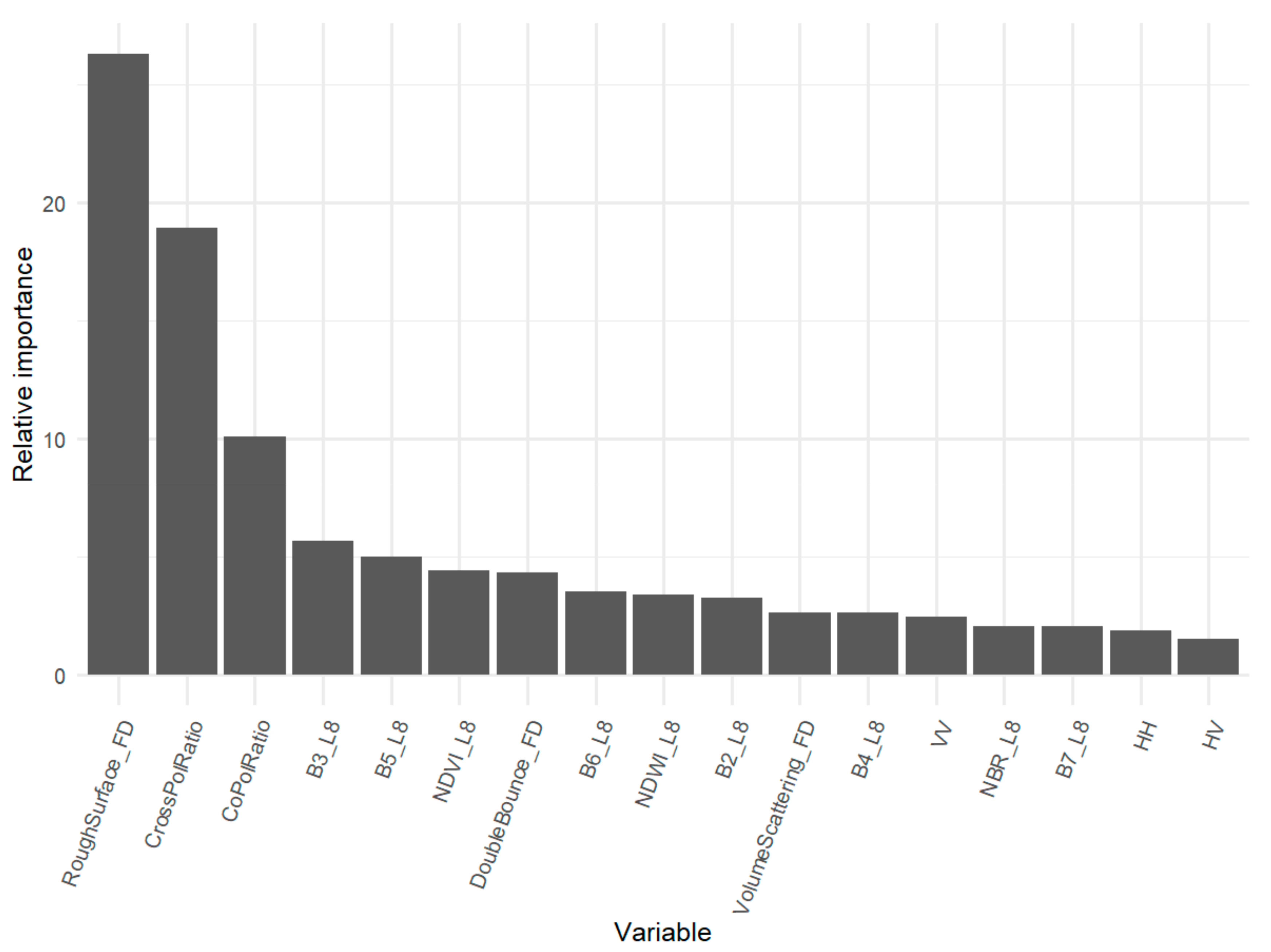
4.1. Relative Importance of EO Inputs

Figure 2 and Figure 3 revealed that polarimetric SAR is much more important for predicting YERA wetland habitat than Landsat-8 optical data. Polarization ratios or decomposition parameters from SAR were shown to have a much larger numerical difference between occupied and unoccupied sites and were much more important in the model. The prediction models were shown to be much more powerful with RADARSAT-2 data included. In fact, it appears that Landsat-8 variables did not improve model performance as a RADARSAT-2-only model generates the same AUC as the RADARSAT-2 + Landsat-8 models. This highlights a limitation of optical data in that it does not penetrate to the vegetation/water surface like SAR. Polarimetric SAR can detect important vegetation flooding and hydrology, due to the 180-degree phase shift of a double bounce SAR return [3,18]. This information is expressed in the cross-pol ratio and double bounce parameters. In addition to the relative importance of RADARSAT-2 data for habitat modeling, the parameters from certain SAR decompositions, such as the Freeman–Durden, can be intuitively related back to on-the-ground habitat characterization, which can be important for conservation efforts.

4.2. Yellow Rail Habitat

Figure 4 can facilitate the interpretation of YERA habitat from EO indices. The relationship between YERA occupancy probability and cross-pol ratio/double bounce shows YERA prefer habitat with flooded vegetation (i.e., there is water/veg interaction in the SAR return). Figure 4a shows a preference for smooth habitat, both vegetation, and topography-wise. Panel (d) of Figure 4 shows an interesting result with YERA preferring habitat with low to moderate amounts of volume scattering. This is most likely associated with graminoid habitat interspersed with tree and shrub habitat that would register high values of volume scattering and open water/barren areas, which would register very low volume scattering values. Landsat-8 index responses to occupancy are harder to interpret, but most bands show higher occupancy at high reflectance. This could be an association with more senescent vegetation (i.e., green vegetation is darker with low reflectance). Figure 7 shows an example of one of these YERA-occupied (verified in the field) habitats which demonstrated one of the highest predicted probability of occupancy hexagons seen in Figure 6. All the wetland habitat associations detected by the EO data are visible: Flooded vegetation, low to moderate biomass, smooth surface, and more senescent vegetation. These interpretations of EO data seem to be consistent with existing descriptions of YERA habitat based on on-the-ground data [10,11], which is a positive finding as EO data does not always match with field observations.

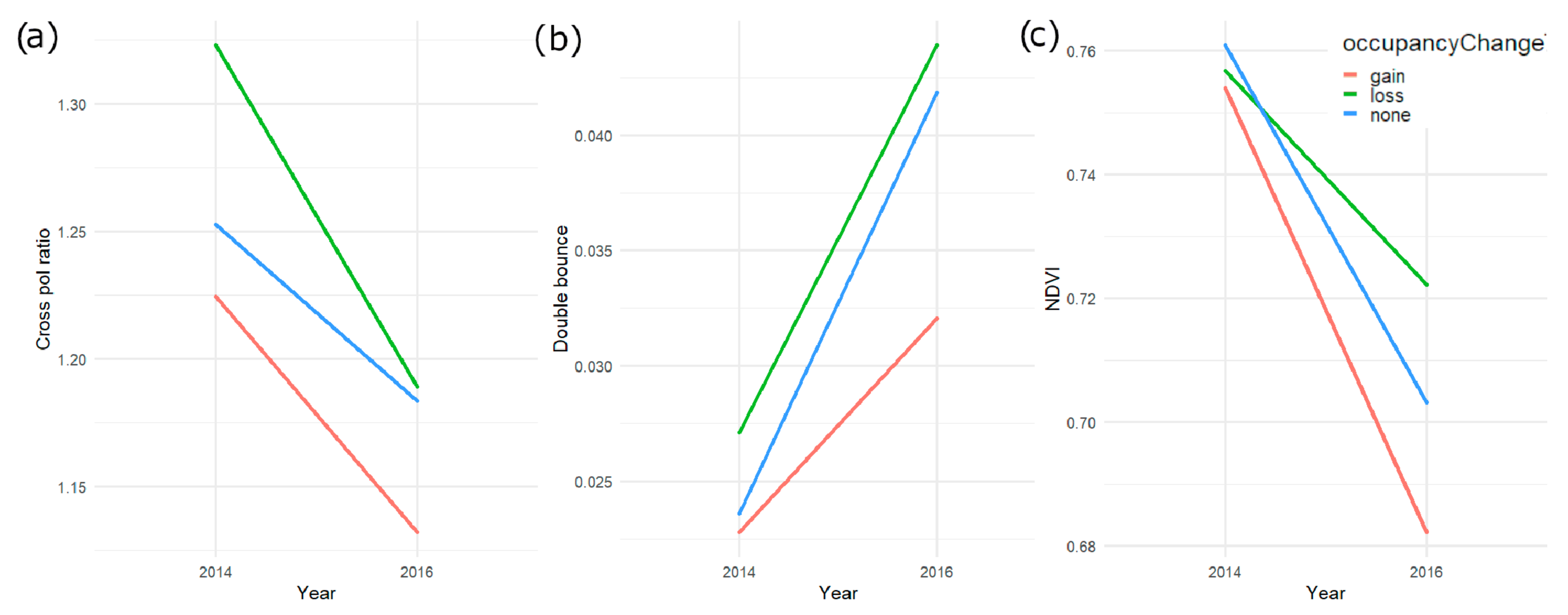
4.3. Monitoring Trends

The yearly trends in YERA habitat from 2014 to 2016 show inconclusive results. All sites, no matter whether the change in occupancy was negative or positive, had the same slope direction. This may indicate that the seasonal changes from August to June produce a stronger signal than the changes from 2014 to 2016. The relative change from 2014 to 2016 may tell us something about changing YERA habitat between years. For example, sites that lost YERA from 2014 to 2016 had a larger drop in cross-pol ratio than sites with no change or gain. This may indicate that sites that lost YERA dried out, corresponding with a lower flooded vegetation signal in 2016; however, this data does not provide conclusive evidence. It is likely that future studies monitoring yearly changes in wetland habitat will need to have consistent image acquisitions dates from year-to-year to capture wetlands in similar seasonal states. Optical data, such as Sentinel-2, may can accomplish this with a 5 day repeat imagery, although, consistent cloud or haze may make this difficult. RADARSAT Constellation Mission (RCM) data and future SAR missions may be a solution as it can provide a rich time series data stack that allows for more control on the observation of seasonal wetland dynamics. Ideally, rather than monitoring indices, multi-year/dynamic occupancy models [34] could be run for YERA or other species based on yearly EO data. This could better capture dynamic wetland habitats and estimate the extinction and colonization rates of many sites. With the increasing availability of high temporal resolution optical and SAR EO data, this will likely be achievable with the right multi-year field data.

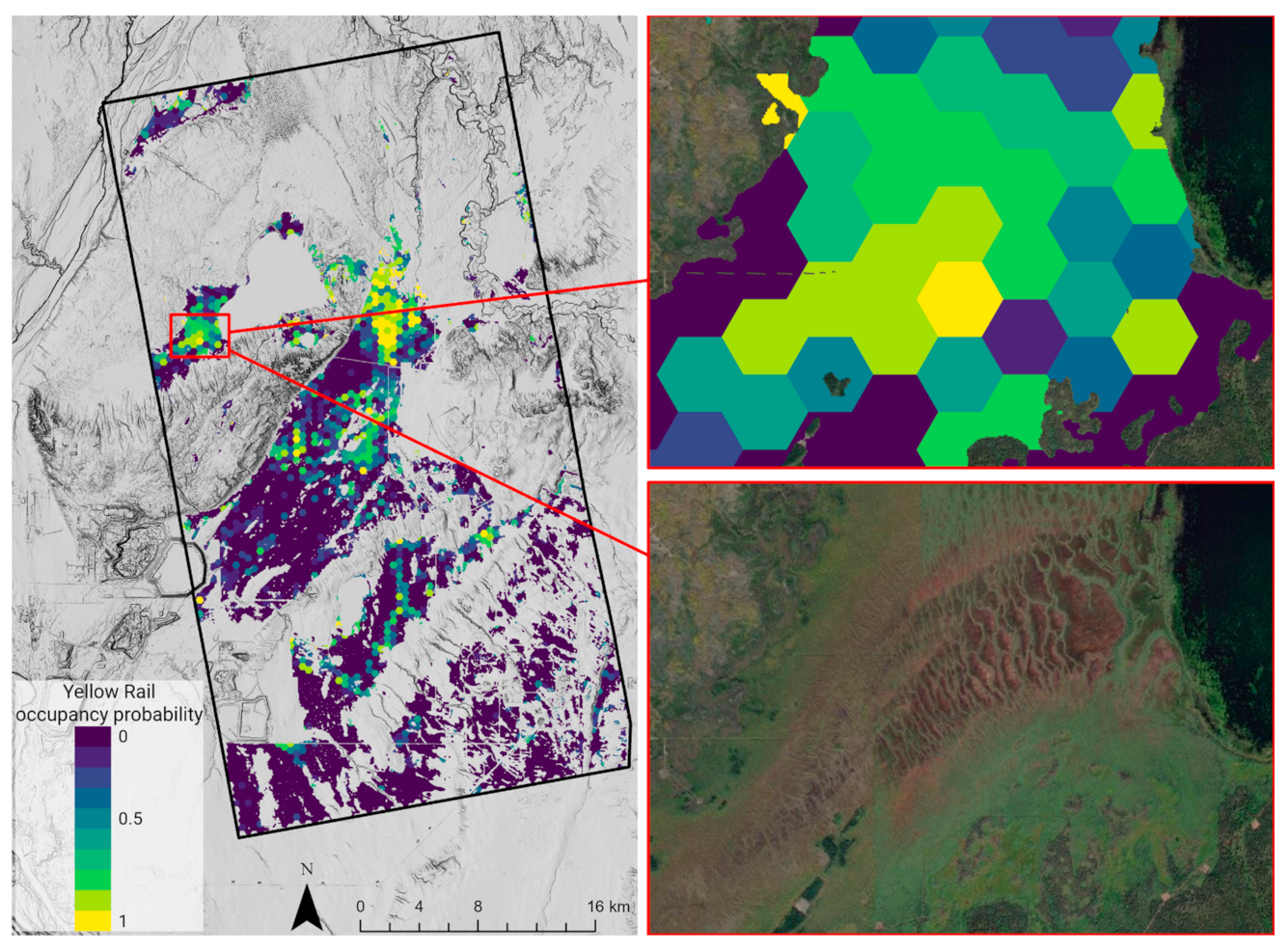
4.4. Habitat Prediction

The prediction of YERA occupancy probability showed good results, with most sites accurately predicting YERA habitat (82%). This prediction came with a 75% true-positive rate and an 86% true-negative rate. We believe this model/similar models should be generalizable to larger areas in the Boreal regions of Canada/North America, as seen in McLeod et al. (2021) [16]. Figure 6 shows that most wetland areas are not suitable habitat highlighting that YERA have very specific habitat needs. All treed wetland areas show near-zero occupancy probability, and most high probability areas were constrained to graminoid wetland areas with a flooded vegetation signature. The prediction results may be biased towards larger YERA habitat patches, due to the large size of the prediction hexagons. Many hexagons can have both treed and graminoid habitat, and therefore, the SAR response for the whole hexagon may not show ideal habitat even though much of the hexagon could be good habitat. A more sensitive model (i.e., fewer false negatives with more false positives) may be more appropriate in many cases for species modeling, especially in areas with development like this study. In the end, the sensitivity can be altered by end-users of these models to shift towards a more desired true positive rate.

Ideally, this prediction map could be updated yearly with new input RADARSAT-2 and Landsat-8 data every year to monitor seasonal changes in the YERA wetland habitat. This study, unfortunately, was data-limited for RADARSAT-2 data (only two available images during the growing season) and could not accomplish yearly monitoring, but moving forward, the RCM data can provide similar data with a dense time series for most areas in Canada.

5. Conclusions

The application of polarimetric RADARSAT-2 data proved to be very powerful for characterizing and predicting YERA habitat. Although optical data from Landsat-8 is likely useful for these applications, it is somewhat limited for detecting flooded vegetation and capturing specific vegetation structures that may be important for wetland-associated wildlife species. Parameters from the RADARSAT-2 Freeman–Durden decomposition provided somewhat intuitive interpretations of YERA habitat, which did match with on-the-ground expected habitat (flooded vegetation, with graminoid vegetation, and more senescent vegetation). Predicting this habitat across a larger area was found to be successful as high probability YERA habitat was constrained to wetland areas corresponding closely to existing descriptions of habitat from the literature (i.e., graminoid, shallow water, senescent vegetation). Results from 2014–2016 habitat trends proved to be somewhat inconclusive. This may be because the magnitude of seasonal change in wetlands (from June to Aug) may have been greater than the magnitude of year-to-year change. This highlights the need for more temporally consistent data with a better temporal resolution for wetland habitat monitoring. Fortunately, this data is now becoming available with the RADARSAT Constellation Mission, which should provide consistent polarimetric SAR data for capturing intra- and inter-year wetland variability. This data can then be a powerful tool for wetland habitat monitoring/conservation efforts.

References

1. He, K.S.; Bradley, B.A.; Cord, A.F.; Rocchini, D.; Tuanmu, M.N.; Schmidtlein, S.; Turner, W.; Wegmann, M.; Pettorelli, N. Will remote sensing shape the next generation of species distribution models? Remote Sens. Ecol. Conserv. 2015, 1, 4–18. [Google Scholar] [CrossRef] [Green Version]
2. Elith, J.; Leathwick, J.R. Species distribution models: Ecological explanation and prediction across space and time. Annu. Rev. Ecol. Evol. Syst. 2009, 40, 677–697. [Google Scholar] [CrossRef]
3. Brisco, B. Mapping and monitoring surface water and wetlands with synthetic aperture radar. Remote Sens. Wetl. Appl. Adv. 2015, 119–136. [Google Scholar] [CrossRef]
4. White, L.; Brisco, B.; Dabboor, M.; Schmitt, A.; Pratt, A. A collection of SAR methodologies for monitoring wetlands. Remote Sens. 2015, 7, 7615–7645. [Google Scholar] [CrossRef] [Green Version]
5. Hird, J.N.; DeLancey, E.R.; McDermid, G.J.; Kariyeva, J. Google earth engine, open-access satellite data, and machine learning in support of large-area probabilistic wetland mapping. Remote Sens. 2017, 9, 1315. [Google Scholar] [CrossRef] [Green Version]
6. Montgomery, J.; Brisco, B.; Chasmer, L.; Devito, K.; Cobbaert, D.; Hopkinson, C. SAR and LiDAR temporal data fusion approaches to boreal wetland ecosystem monitoring. Remote Sens. 2019, 11, 161. [Google Scholar] [CrossRef] [Green Version]
7. DeLancey, E.R.; Simms, J.F.; Mahdianpari, M.; Brisco, B.; Mahoney, C.; Kariyeva, J. Comparing deep learning and shallow learning for large-scale wetland classification in Alberta, Canada. Remote Sens. 2020, 12, 2. [Google Scholar] [CrossRef] [Green Version]
8. Wells, J.V. Boreal Birds of North America: A Hemispheric View of Their Conservation Links and Significance; University of California Press: Berkley, CA, USA, 2011. [Google Scholar]
9. Wetlands International. Waterbird Population Estimates. Available online: http://wpe.wetlands.org/ (accessed on 10 January 2019).
10. Leston, L.B.T. Yellow Rail (Coturnicops Noveboracensis), version 2.0; Cornell Lab of Ornithology: Ithaca, NY, USA, 2015. [Google Scholar]
11. Robert, M.; Laporte, P. Numbers and movements of yellow rails along the St. Lawrence River, Quebec. Condor 1999, 101, 667–671. [Google Scholar] [CrossRef]
12. Amani, M.; Mahdavi, S.; Afshar, M.; Brisco, B.; Huang, W.; Mohammad Javad Mirzadeh, S.; White, L.; Banks, S.; Montgomery, J.; Hopkinson, C. Canadian wetland inventory using google earth engine: The first map and preliminary results. Remote Sens. 2019, 11, 842. [Google Scholar] [CrossRef] [Green Version]
13. Pouliot, D.; Latifovic, R.; Pasher, J.; Duffe, J. Assessment of convolution neural networks for wetland mapping with landsat in the central Canadian boreal forest region. Remote Sens. 2019, 11, 772. [Google Scholar] [CrossRef] [Green Version]
14. Mao, D.; Wang, Z.; Du, B.; Li, L.; Tian, Y.; Jia, M.; Zeng, Y.; Song, K.; Jiang, M.; Wang, Y. National wetland mapping in China: A new product resulting from object-based and hierarchical classification of Landsat 8 OLI images. ISPRS J. Photogramm. Remote Sens. 2020, 164, 11–25. [Google Scholar] [CrossRef]
15. Millard, K.; Richardson, M. Wetland mapping with LiDAR derivatives, SAR polarimetric decompositions, and LiDAR–SAR fusion using a random forest classifier. Can. J. Remote Sens. 2013, 39, 290–307. [Google Scholar] [CrossRef]
16. McLeod, L.J.; DeLancey, E.R.; Bayne, E.M. Spatially Explicit Abundance Modelling of a Highly Specialized Wetland Bird using Sentinel-1 and Sentinel-2. Candian J. Remote Sens. 2021, in press. [Google Scholar]
17. Schmitt, A.; Brisco, B. Wetland monitoring using the curvelet-based change detection method on polarimetric SAR imagery. Water 2013, 5, 1036–1051. [Google Scholar] [CrossRef]
18. Brisco, B.; Schmitt, A.; Murnaghan, K.; Kaya, S.; Roth, A. SAR polarimetric change detection for flooded vegetation. Int. J. Digit. Earth 2013, 6, 103–114. [Google Scholar] [CrossRef]
19. Freeman, A.; Durden, S.L. A three-component scattering model for polarimetric SAR data. IEEE Trans. Geosci. Remote Sens. 1998, 36, 963–973. [Google Scholar] [CrossRef] [Green Version]
20. Wellmann, T.; Lausch, A.; Scheuer, S.; Haase, D. Earth observation based indication for avian species distribution models using the spectral trait concept and machine learning in an urban setting. Ecol. Indic. 2020, 111, 106029. [Google Scholar] [CrossRef]
21. Bino, G.; Levin, N.; Darawshi, S.; Van Der Hal, N.; Reich-Solomon, A.; Kark, S. Accurate prediction of bird species richness patterns in an urban environment using Landsat-derived NDVI and spectral unmixing. Int. J. Remote Sens. 2008, 29, 3675–3700. [Google Scholar] [CrossRef]
22. St-Louis, V.; Pidgeon, A.M.; Kuemmerle, T.; Sonnenschein, R.; Radeloff, V.C.; Clayton, M.K.; Locke, B.A.; Bash, D.; Hostert, P. Modelling avian biodiversity using raw, unclassified satellite imagery. Philos. Trans. R. Soc. B Biol. Sci. 2014, 369, 20130197. [Google Scholar] [CrossRef] [PubMed] [Green Version]
23. Buermann, W.; Saatchi, S.; Smith, T.B.; Zutta, B.R.; Chaves, J.A.; Milá, B.; Graham, C.H. Predicting species distributions across the Amazonian and Andean regions using remote sensing data. J. Biogeogr. 2008, 35, 1160–1176. [Google Scholar] [CrossRef]
24. Farrell, S.; Collier, B.; Skow, K.; Long, A.; Campomizzi, A.; Morrison, M.; Hays, K.; Wilkins, R. Using LiDAR-derived vegetation metrics for high-resolution, species distribution models for conservation planning. Ecosphere 2013, 4, 1–18. [Google Scholar] [CrossRef]
25. Chen, F.; Guo, H.; Ishwaran, N.; Zhou, W.; Yang, R.; Jing, L.; Chen, F.; Zeng, H. Synthetic aperture radar (SAR) interferometry for assessing Wenchuan earthquake (2008) deforestation in the Sichuan giant panda site. Remote Sens. 2014, 6, 6283–6299. [Google Scholar] [CrossRef] [Green Version]
26. Evans, T.L. Habitat Mapping of the Brazilian Pantanal Using Synthetic Aperture Radar Imagery and Object Based Image Analysis; University of Victoria: Victoria, BC, Canada, 2013. [Google Scholar]
27. Battaglia, M.J.; Banks, S.; Behnamian, A.; Bourgeau-Chavez, L.; Brisco, B.; Corcoran, J.; Chen, Z.; Huberty, B.; Klassen, J.; Knight, J. Multi-source eo for dynamic wetland mapping and monitoring in the great lakes basin. Remote Sens. 2021, 13, 599. [Google Scholar] [CrossRef]
28. Hedley, R.; McLeod, L.; Yip, D.; Farr, D.; Knaga, P.; Drake, K.; Bayne, E. Modeling the occurrence of the Yellow Rail (Coturnicops noveboracensis) in the context of ongoing resource development in the oil sands region of Alberta. Avian Conserv. Ecol. 2020, 15, 10. [Google Scholar] [CrossRef]
29. Natural Regions Committee. Natural Regions and Subregions of Alberta. Compiled by DJ Downing and WW Pettapiece. Government of Alberta; Government of Alberta Pub: Edmonton, AB, Canada, 2006. [Google Scholar]
30. Yip, D.; Leston, L.; Bayne, E.; Sólymos, P.; Grover, A. Experimentally derived detection distances from audio recordings and human observers enable integrated analysis of point count data. Avian Conserv. Ecol. 2017, 12, 1–10. [Google Scholar] [CrossRef] [Green Version]
31. Thuiller, W.; Brotons, L.; Araújo, M.B.; Lavorel, S. Effects of restricting environmental range of data to project current and future species distributions. Ecography 2004, 27, 165–172. [Google Scholar] [CrossRef]
32. Gorelick, N.; Hancher, M.; Dixon, M.; Ilyushchenko, S.; Thau, D.; Moore, R. Google Earth Engine: Planetary-scale geospatial analysis for everyone. Remote Sens. Environ. 2017, 202, 18–27. [Google Scholar] [CrossRef]
33. Elith, J.; Leathwick, J.R.; Hastie, T. A working guide to boosted regression trees. J. Anim. Ecol. 2008, 77, 802–813. [Google Scholar] [CrossRef]
34. MacKenzie, D.I.; Bailey, L.L.; Hines, J.E.; Nichols, J.D. An integrated model of habitat and species occurrence dynamics. Methods Ecol. Evol. 2011, 2, 612–622. [Google Scholar] [CrossRef]
Figure 1. Study area. Panel (a) shows the true color image of the area with field sites in green (YERA present) and grey (YERA absent), panel (b) shows the elevation of the area, and panel (c) show the study area located in relation to the rest of western Canada.
Water 13 02327 g001
Figure 2. Box plots showing the difference between the EO inputs and YERA site occupancy. Panel (a) is the rough surface component of the Freeman-Durden, (b) is the double bounce component of the Freeman-Durden, (c) is the cross polarization ratio, and (d) is NDVI.
Water 13 02327 g002
Figure 3. The relative importance of inputs in the prediction model.
Water 13 02327 g003
Figure 4. Response plots (how occupancy probability changes with changing EO values) for six potential YERA model inputs. (a) Rough surface (b) cross polarization ratio, (c) double bounce, (d) volume scattering, (e) band 3, (f) band 6.
Water 13 02327 g004
Figure 5. Yearly trends in three EO indies between 2014 and 2016 for three sites types. (a) cross polarization ratio (b) double bounce, and (c) NDVI.
Water 13 02327 g005
Figure 6. Hexagonal YERA occupancy probability for the study area. Yellows represent high YERA occupancy probability, and darker colors represent low probabilities. Insets on the right zoom in on areas with suitable YERA habitat (center and graminoid areas of wetland habitat) and poor habitat (edge/treed wetland).
Water 13 02327 g006
Figure 7. Field site picture capture in May 2014. This site is frequently occupied by YERA and had one of the highest predicted occupancy probabilities.
Water 13 02327 g007