
Uncertainty of Intensity-Duration-Frequency Curves Due to Adoption or Otherwise of the Temperature Climate Variable in Rainfall Disaggregation


1
Department of Water Resources Engineering, Mustansiriyah University, Baghdad 10001, Iraq
2
Department of Civil Engineering, Mustansiriyah University, Baghdad 10001, Iraq
*
Author to whom correspondence should be addressed.
Water 2021, 13(17), 2337; https://doi.org/10.3390/w13172337
Submission received: 7 July 2021
/
Revised: 19 August 2021
/
Accepted: 19 August 2021
/
Published: 26 August 2021
(This article belongs to the Section Hydrology)
Abstract
:Most areas around the world lack fine rainfall records which are needed to derive Intensity-Duration-Frequency (IDF) curves, and those that are available are in the form of daily data. Thus, the disaggregation of rainfall data from coarse to fine temporal resolution may offer a solution to that problem. Most of the previous studies have adopted only historical rainfall data as the predictor to disaggregate daily rainfall data to hourly resolution, while only a few studies have adopted other historical climate variables besides rainfall for such a purpose. Therefore, this study adopts and assesses the performance of two methods of rainfall disaggregation one uses for historical temperature and rainfall variables while the other uses only historical rainfall data for disaggregation. The two methods are applied to disaggregate the current observed and projected modeled daily rainfall data to an hourly scale for a small urban area in the United Kingdom. Then, the IDF curves for the current and future climates are derived for each case of disaggregation and compared. After which, the uncertainties associated with the difference between the two cases are assessed. The constructed IDF curves (for the two cases of disaggregation) agree in the sense that they both show that there is a big difference between the current and future climates for all durations and frequencies. However, the uncertainty related to the difference between the results of the constructed IDF curves (for the two cases of disaggregation) for each climate is considerable, especially for short durations and long return periods. In addition, the projected and current rainfall values based on disaggregation case which adopts historical temperature and rainfall variables were higher than the corresponding projections and current values based on only rainfall data for the disaggregation.
1. Introduction
Intensity-Duration-Frequency (IDF) curves indicate maximum rainfall events for certain frequencies and durations and this information is crucial for the flood analysis step in designing hydrosystems. There is an increasing trend in the maximum rainfall values with daily and sub-daily timescales in different regions of the world and such rainfall values are comparable to the amount displayed by the IDF curves [1,2,3,4,5]. However, due to global warming and non-stationarity, the return period for a specific rainfall event varies over time [6,7,8]. According to the Intergovernmental Panel on Climate Change (IPCC) [9], the return period for annual maximum (AM) precipitation will decrease significantly by the end of the 21st century, extreme rainfall events will occur more frequently, and consequently, the risk of flooding will increase [10].
Thus, action needs to be taken to ensure that stormwater collection systems for urban areas can accommodate these anticipated changes in extreme rainfall events [11]. To date, historical IDF curves are the main tool to design such water collection systems. However, due to climate change, these curves need to be amended [12]. Therefore, there is an urgent need to (1) check whether the current IDF curves used in the design of urban stormwater collection systems are still appropriate in terms of their level accuracy and uncertainty in light of the impact of climate change and (2) consider future projections based on sub-daily rainfall durations (hourly or sub-hourly) for the design of these curves.
For an urban watershed, it is necessary to have rainfall data with fine temporal resolution (i.e., hourly or sub-hourly) in order for a hydrological model to produce reliable outcomes [13,14]. However, in many parts of the world, precipitation records are normally available only as daily data, and only a few regions have hourly data, which means that fine-resolution observations are not often available. In addition, the outputs of climate models are mostly on a daily scale. Thus, to evaluate the sensitivity and strength of stormwater drainage systems for urban areas, it is important to disaggregate precipitation data for both current and future climates to a fine temporal resolution.
In the literature, a number of different disaggregation techniques have been proposed to overcome the issue of coarse temporal resolution, such as Poisson-cluster models [15,16,17,18,19], generalized linear models [13,20], random cascade models [21,22,23,24], and nonparametric methods such as the artificial neural network [25], K-nearest neighbor (KNN) technique [26,27,28,29], and method of fragments (MoF) framework [30,31,32,33]. Some of the above techniques consider only the rainfall variable (i.e., historical rainfall data) to disaggregate the current and future rainfall data [33,34,35,36,37]. Other techniques take into account other climate variables (e.g., temperature, relative humidity, etc.) in addition to the rainfall variable for the rainfall disaggregation [38,39,40].
Alam and Elshorbagy [41] and Uraba et al. [42] used the KNN method to disaggregate future daily rainfall to hourly and sub-hourly scales using only historical rainfall as the predictor for the disaggregation. The authors focused on finding the proper window size to find the AM rainfall values and compared them with the historical AMs. Although it is important to find proper values for AMs, it is just as important to identify the rainfall temporal pattern. The full rainfall temporal pattern at high resolution can be obtained by disaggregating low-resolution rainfall data. However, disaggregating future rainfall based on historical rainfall alone may not produce the proper rainfall temporal pattern. Due to climate change, the atmosphere is becoming warmer. Thus it follows that the rainfall temporal pattern for the warmer days in the historical rainfall data will reflect the future climate pattern [39].
When designing an urban hydrosystem, a flood analysis needs to be undertaken, and the accuracy of such an analysis depends on the continuous simulation of rainfall time series [37]. However, it can be argued that although the continuous simulation of a long rainfall time series (i.e., disaggregated data) will lead to the production of an accurate design for an urban drainage network, such a simulation requires a long computational time and the output needs to be subjected to statistical post-processing [11,43]. Thus, it is more practical to focus on the AMs and adopt a design storm with a certain temporal pattern that can later be used in an urban drainage model.
However, one of the drawbacks of design storms is that they are based on a fixed temporal pattern of rainfall that does not take into account the impacts of climate change. In addition, Wasko and Sharma [44] showed that the relationship between rainfall and temperature, which is known as scaling, is important not only for overall rainfall volume, but also for rainfall fractions (i.e., the segments of the rainfall temporal pattern) because each fraction within a rainfall temporal pattern scales differently with temperature. In regard to the area under investigation in the current study, Fadhel et al. [45] showed that as the climate warms, the peak fraction within a storm event become peakier while the non-peak fractions become less for different durations with and without seasonal separation.
Thus, from the above discussion, it can be seen that whether the designer of an urban drainage network adopts a continuous simulation or a design storm, the most important consideration in both of these approaches is the rainfall temporal pattern. Consequently, using only historical rainfall without temperature for the disaggregation of future rainfall may not lead to an output that reflects the proper rainfall temporal pattern of the future climate.
As previously mentioned, some of the earlier studies used more than one climate variable for disaggregation, especially when disaggregating daily rainfall to a sub-hourly (5 min) scale. However, when disaggregating daily rainfall to an hourly timescale, most of the previous studies used only historical rainfall. Thus, this study aims to determine whether it is necessary to adopt a historical temperature variable alongside historical rainfall data to disaggregate daily rainfall data to an hourly resolution or not. To achieve this aim, the difference in the results of the constructed IDF curves for two cases is studied. One case involves using the rainfall and temperature climate variables for the disaggregation and the other case involves using the rainfall climate variable alone (i.e., without temperature). The disaggregation is done for both the current and future climates and from a daily to an hourly timescale. Thus, the focus of this study is different from that of previous studies which concentrated on finding and comparing the uncertainty in the IDF curves that results from the application of different disaggregation methods. Here, the focus is instead on the uncertainty in the IDF curves that may result from using one or more than one climate variable as the predictor for the disaggregation of coarse rainfall data to fine-resolution data, especially from a daily to an hourly scale.
Thus, the aims of this study are to (1) produce continual hourly precipitation records for the future period 2069–2098 and derive future IDF curves; (2) distinguish the difference between the IDF curve results for the two climates (current and future) generated by the two cases of rainfall disaggregation—one with and one without the inclusion of the temperature variable alongside the rainfall variable, and (3) quantify the uncertainty associated with the derived IDF curves for both the observed current and modeled future climate which results from the two cases of disaggregation.
2. Materials and Methods
2.1. Study Area and Data
2.1.1. Metrological Data
The study area is a small urban catchment approximately 12 km × 5 km in size located in West Yorkshire, in the north of England in the United Kingdom (UK). The Centre of Ecology and Hydrology Gridded Estimates of Areal Rainfall (CEH_GEAR) created a gridded daily precipitation product for the whole of the UK for the period 1890–2014 [46]. This gridded rainfall dataset has a space scale of 1 km2 and is dependent on different densities of station for different periods of time. For instance, there were approximately 4400 rainfall stations during the period 1961–2000 with an average of one station for each 49 km2 over the whole of the UK [47], while the maximum station densities were for the year 1974 with around 6250 stations [48]. For the current study, the observed (historical) rainfall data for the study area was extracted from the CEH_GEAR dataset for the period 1950–2014.
In addition, composite radar rainfall data for the study area was obtained from the UK Met Office radar network through the British Atmospheric Data Centre. The composite radar data has a space scale and a timescale of 1 km and 5 min, respectively. A radar grid of 60 km2 covers the study area and is within the scope of three single-polarization C-band weather radars. These radars are Hameldon Hill, Ingham, and High Moorsley, which are 30 km, 90 km, and 95 km away from the study area, respectively [49]. The radar rainfall data has different sources of error which have previously been quality controlled and corrected [50]. Yet, more examination and post-processing of the radar rainfall data was done in the current study by adopting the procedure in Fadhel et al. [51]. Furthermore, the radar data were aggregated from 5 min to an hourly timescale for the period January 2006 to May 2016, and used to disaggregate the observed and future rainfall from daily to hourly durations.
As regards to the air temperature data, this study adopted the gridded daily temperature data provided by the Climate Hydrology and Ecology Research Support System meteorology dataset (1961–2015) (CHESS-met), which is at a 1 km space scale. The CHESS-met temperature was derived for a reference height of 1.2 m by Robinson et al. [52]. First, the authors modify the resolution of the MORECS air temperature from a 40 km to a 1 km space scale by adopting the bicubic spline method for the interpolation. Then they used the integrated hydrological digital terrain model to fit the interpolated data at each pixel of the 1 km grid to its elevation. For the current study, the observed temperature data for the period 1985–2014 was extracted from the CHESS-met dataset. The CHESS-met temperature data were used to correct the bias for the climate temperature data (Section 2.2.1) and to disaggregate the rainfall data as well (Section 2.2.2).
2.1.2. Climate Data
The climate data provided by the Met Office Hadley Centre HadRM3 dataset was adopted in this study. The Met Office Hadley Centre used the global climate model HadCM3 for its regional climate model HadRM3 in order to predict climate conditions for the future at the regional level [53]. The regional climate model (RCM) data consist of an 11-member ensemble that were derived for the historical emissions scenario, SRES A1B, by perturbing 10 members to atmospheric parametrizations with different perturbations and leaving one unperturbed member [53]. The climate data time series can be acquired from the HadRM3 Perturbed Physics Experiment Dataset (HadRM3-PPE-UK) for the period 1950–2100 with a 25 km and a daily spatial and temporal resolution, respectively.
The study area is situated among two climate grids and each grid has a space scale of 25 km. For the two grids, the future temperature data that were modeled at a 1.5 m reference height for the period 2069–2098 were bias corrected based on the period 1985–2014.
However, the modeled precipitation produced by the HadRM3 dataset showed systematic discrepancies compared to the observations, especially for the historical period pre-2000. Therefore, the future flow climate data provided by the Centre for Ecology and Hydrology modify and spatially downscale the modeled precipitation from 25 km down to 1 km [54,55]. Nevertheless, although Newton et al. [54] bias corrected and downscaled the modeled precipitation, Prudhomme et al. [55] stated that the data still had some inconsistencies as compared with the observed data. Thus, in the current study, the observed rainfall data for the period 1950–2014 and at a 1 km space scale were adopted to bias correct the future precipitation data for the period 2069–2098, as explained in Section 2.2.1.
2.2. Methodology
2.2.1. Statistical Bias Correction Method
The distribution-based scaling (DBS) approach was adopted in this study to correct the bias of the two climate variables (precipitation and temperature) modeled by the daily RCM [56].
First, the double gamma distribution was used to separate the precipitation distribution into two parts based on the 95th percentile. This separation technique was performed for every month over the calendar year to map the quantiles of the observed and simulated data, which helped to define the main features of both extreme and normal precipitations. The density distribution of the applied double gamma distribution is expressed as:
where Γ, α, and β are the gamma function, shape parameter, and scale parameter, respectively.
Second, before correcting the bias of the climate temperature data, the spatial resolution of the observed and modeled temperature datasets had to be adjusted. This was done by spatially upscaling the observed temperature data from 1 km to 25 km by using a simple averaging method, which resulted in two grids covering the study area that matched the RCM temperature grids. Then, the DBS method was applied to correct the bias of the climate temperature data to the upscaled observed data by using Gaussian distribution. Like Yang et al. [56], the seasonal variation was taken into account by a moving window of 15 days to smooth the mean and standard deviation of daily temperature. The variation was further smoothed by using Fourier series with five harmonics. In addition, the climate temperature data were corrected without dependence between precipitation and temperature (i.e., wet-dry day separation) because Olsson et al. [57] proved that the modeled temperature data could be bias corrected with and without wet-dry day separation.
To correct the bias of the model future projection, it is necessary to identify the cumulative distribution function (CDF) of the future period by finding the corresponding percentile values of the model in the reference period. Then, the bias-corrected future value can be found by using the observation CDF to find the value of the climate variable for the same future CDF. This relationship takes the following form:
where and denote the gamma CDF and its inverse function, respectively, and is the bias-corrected data in the baseline period. The parameters associated with the RCM simulated and observed precipitation are denoted by the subscripts mod and obs, respectively.
The main drawback of this bias correction procedure is assumption that there is a constant bias between the reference and future periods. However, Fadhel et al. [38] investigated the uncertainty in constructed future IDF curves that results from the use of different reference periods and found that an ensemble approach can be used to address this problem. Thus, this study adopted the Fadhel et al. [38] procedure for bias correction and used an ensemble of reference periods to bias correct one RCM to thereby mitigate the uncertainty that may have emerged from the use of one reference period for bias correction.
For this analysis, the observed and modeled rainfall time series for the period 1950–2014 were split into 8 sub-periods. Each sub-period had a specified length of 30 years and a moving window of 5 years that moved from the first to the last sub-period. Thus, all the ensemble members of the future RCM for the period 2069–2098 were bias corrected 8 times according to the 8 reference periods.
However, because the purpose of the study was to evaluate the uncertainty of the derived future IDF curves that may outcome from disaggregating the rainfall data with and without adopting the temperature variable for the disaggregation, the future climate temperature data for the period (2096–2098) were bias corrected depending on one reference period. The most recent reference period was adopted to bias correct the climate temperature variable (i.e., 1985–2014) because previous studies showed that the atmosphere is becoming warmer as compared to historical records [39]. Thus, using the most recent reference period (i.e., the warmest) to correct the bias of the modeled temperature and changing the reference period used to correct the bias of the modeled rainfall (i.e., 8 reference periods) will help to capture the temporal pattern of future rainfall based on the rainfall pattern of the warmer days in the historical data [39].
2.2.2. Disaggregation Methods
Due to climate change, the patterns of future rainfall can be reflected by the pattern of warmer days in the historical record [39]. Thus, the adoption of historical rainfall alone as a predictor to disaggregate future rainfall may not accurately predict the future rainfall temporal pattern [38]. However, previous studies adopted historical rainfall as the sole predictor for the disaggregation of future rainfall from daily to hourly and sub-hourly (i.e., 5 min) timescales. Therefore, this study investigated how the disaggregated future rainfall affected the constructed future IDF curves when the disaggregation was performed with and without using historical temperature as a second predictor alongside historical rainfall.
For the first method in this study, that is, for rainfall disaggregation using both the historical temperature and historical rainfall variables, this study adopted an algorithm that integrates both the nonparametric prediction (NPRED) model and the MoF framework [38,40]. The logic of partial informational correlation is employed in the NPRED model to determine the system predictors, and it predicts the responses by using the KNN regression formula depending on partial weights and the weighted Euclidean distance. The KNN regression estimator can be expressed as:
where E(X\Z) represents the conditional expectation of a response (X) conditional to a given predictor set (Z), ki represents the number of observations, the subscript j ranging from 1 to K, where K is the maximum number of neighbors permissible, i = 1 … n, are a sample of observations.
The NPRED model is freely available from the NPRED R-package open source [58]. As the NPRED model can only predict the responses, the MoF framework, which was developed by Westra et al. [33] and Mehrotra et al. [59] based on the assumption of historical climate, can be used to determine the whole temporal pattern of sub-daily rainfall [39]. The MoF framework uses historical observations on daily rainfall and other atmospheric covariates (i.e., the temperature variable in this study) to resample the fragments for the sub-daily scale. In this study, the current observed and future modeled rainfall data for the periods 1985–2014 and 2069–2098, respectively, were disaggregated from a daily to an hourly timescale.
For the same research area, Fadhel et al. [38] showed that using all the data for rainfall disaggregation is better than using seasonal separation. Thus, the NPRED algorithm was used to predict the maximum 1 h storm fraction without seasonal separation of the climate data.
The procedure used by the algorithm for rainfall disaggregation consists of the following steps:
- By using the historical hourly rainfall data (i.e., the sum of 5 min radar data), find the fraction of 1 h, that is, the ratio between the maximum 1 h storm fraction on a particular day divided by the total amount of rainfall value for that day;
- By using the NPRED tool, fit a model between the predictor variables, which are daily temperature and daily rainfall (i.e., the sum of 5 min radar data), and the response, which is the 1 h fraction determined from step 1;
- To predict the future 1 h fraction, apply the model that resulted from step 2 to the predictors of the future climate data;
- To find the analogue for the future atmospheric state which was projected in step 3, apply the MoF framework with an optimal window size 15 [28] to search the historical data for such an analogue. Then, the rainfall temporal pattern can be resampled from one of these days (see Equation (2) in [33]).
For the second method in this study, that is, for future rainfall disaggregation using only historical rainfall as the predictor (i.e., without using the temperature variable), this study employed the widely adopted KNN method, with an optimal window size of 15 in line with Sharif and Burn [46]. For more details on the application of this method in this area of research, see [26,27,29].
In the remainder of this paper, the rainfall disaggregation by the NPRED-MoF algorithm (i.e., by using the two climate variables of temperature and rainfall as the predictor variables) is denoted as case 1, while disaggregation by the KNN method (i.e., using only the rainfall variable as the predictor without temperature) is denoted as case 2.
2.2.3. Creation of IDF Curves
Based on the assessment of three different goodness-of-fit tests (i.e., the Kolmogorov–Smirnov, Anderson–Darling, and Chi-squared tests), the extreme value (EV) distribution was found to be the best probability distribution at the 95% significant level for the study area. The derivation process of the goodness-of-fit tests followed the standard procedure [60], and is therefore not described here. The cumulative density function of the EV distribution is defined as:
where, µ and σ are the location parameter, and scale parameter, respectively.
The IDF curves were created based on the EV distribution for the AM series, and the parameters of the EV distribution were obtained by using the maximum likelihood estimates method.
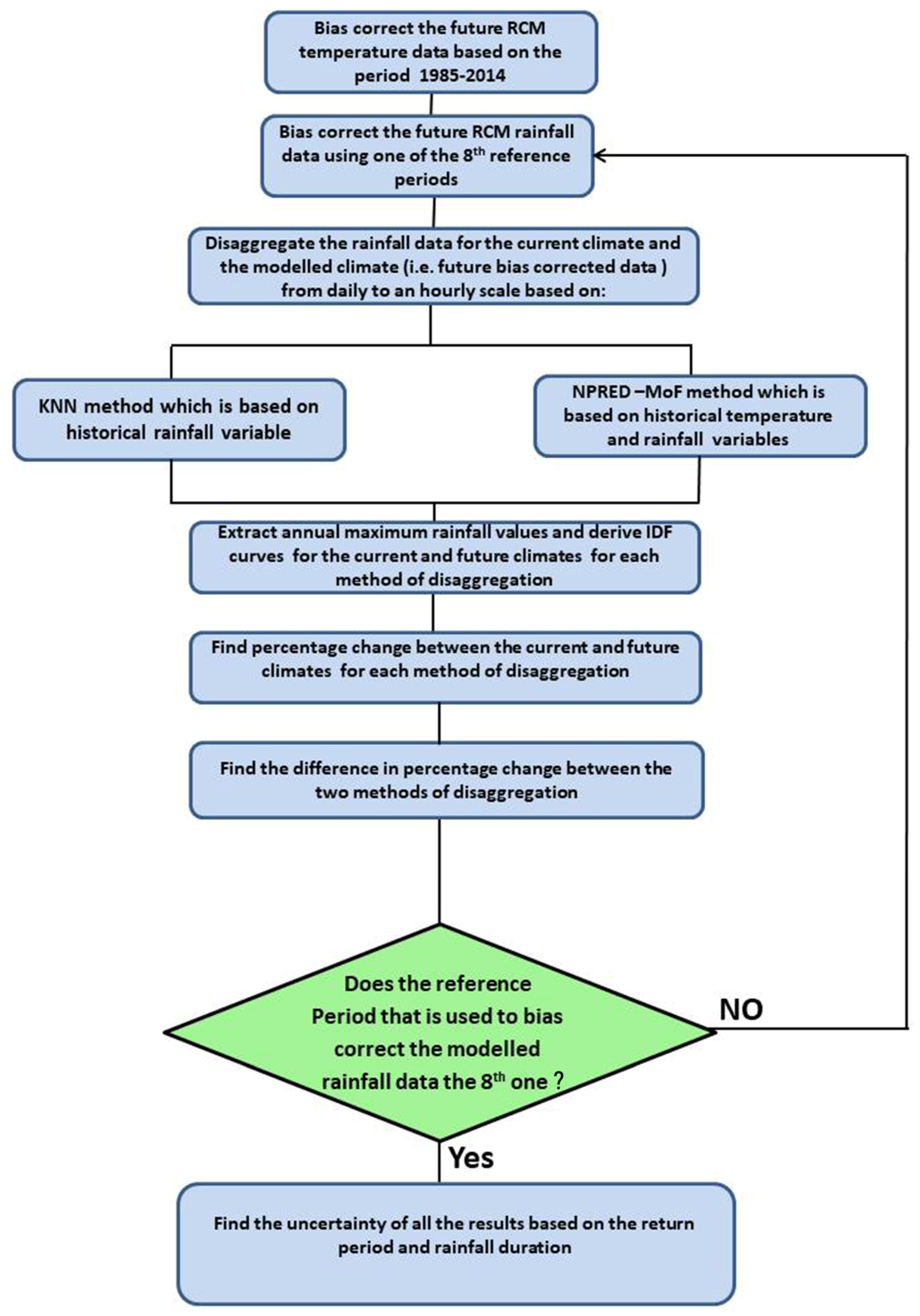
The procedure of creating future IDF curves is explained briefly below and shown in Figure 1:
- Use a specific reference period to correct the bias of the future modeled rainfall data for the period 2069–2098.
- Disaggregate the future bias-corrected RCM from a daily to a 1 h timescale using the NPRED-MoF algorithm one time and the KNN method another time, and determine the areal average of the future hourly disaggregated rainfall data for the study area.
- Aggregate the disaggregated future hourly rainfall intensity to five durations (1, 3, 6, 12, and 24 h) depending on the concentration time. Due to the high uncertainty that may result from the methods that can be used to calculate the concentration time [61,62,63], it was noticed that the value of concentration time for the study area can vary depending on the method used for such a purpose. Thus, the value that fit to the purpose of the study was adopted (i.e., a concentration time of 1 h) [62]. Thus, the aggregation into five rainfall durations had to be done by applying a moving window equal to the concentration time (i.e., 1 h) to the full hourly disaggregated time series.
- Derive AM series of rainfall intensity for each duration then apply EV distribution for the derived series to find the rainfall depths for six different return periods (2, 5, 10, 25, 50, and 100 years).
The above procedure is repeated to create IDF curves for all the eight reference periods.
3. Results and Discussion
3.1. Rainfall Disaggregation
As mentioned earlier, this study used two cases to disaggregate rainfall data from a daily to an hourly timescale. For case 1, the NPRED-MoF algorithm was adopted, in which the temperature variable as well as the rainfall variable was used for the disaggregation. For case 2, the conventional KNN method was used to disaggregate the rainfall by using the rainfall variable alone (i.e., without temperature). The effect of the two methods on the disaggregation of rainfall data from a daily to an hourly timescale is discussed below for three examples of the future climate, each of which used a different RCM ensemble member.
The first example was a climate ensemble member for the year 2074 and a daily rainfall value of 49.91 mm. When this daily rainfall value was disaggregated to an hourly scale by using the two cases of rainfall disaggregation, case 1 gave a rainfall temporal pattern with a peak of 25.1 mm and case 2 gave a temporal pattern with a peak of 13.6 mm. (It is worth noting that the peaks in this example and the rest of the examples in this section were the AM values for the duration of 1 h since the concentration time was found to be 1 h). Hence it was clear that the difference between the two peaks (i.e., the AMs) of the hourly disaggregated data produced by the two cases of disaggregation for this future climate example was considerable and would also lead to big differences in the derived IDF curves.
In the second RCM ensemble example, in contrast to the previous example where the peak of rainfall temporal pattern for the disaggregated data produced by case 1 was lower than that produced by case 2. Such disaggregation was for a future daily rainfall value of 105.3 mm and the year 2094 that gave peaks (which are the same as the AMs) of 28 mm and 45.3 mm when subjected to case 1 and case 2 disaggregation, respectively.
Interestingly, in the third RCM ensemble example, cases 1 and 2 produced the same rainfall temporal pattern, and consequently, the same peaks and AMs for the disaggregated data for the year 2084, as well as a daily rainfall value of 58 mm that gave a peak of 12.88 mm.
It is clear from the above examples that the differences in the AM values that resulted from the two cases of disaggregation were significant. It is also logical to conclude that such differences would highly affect the derived IDF curves for the current and future climates and consequently produce high uncertainty. Furthermore, this uncertainty resulted not just from the disaggregation method, but from the number of climate variables that were used for the disaggregation.
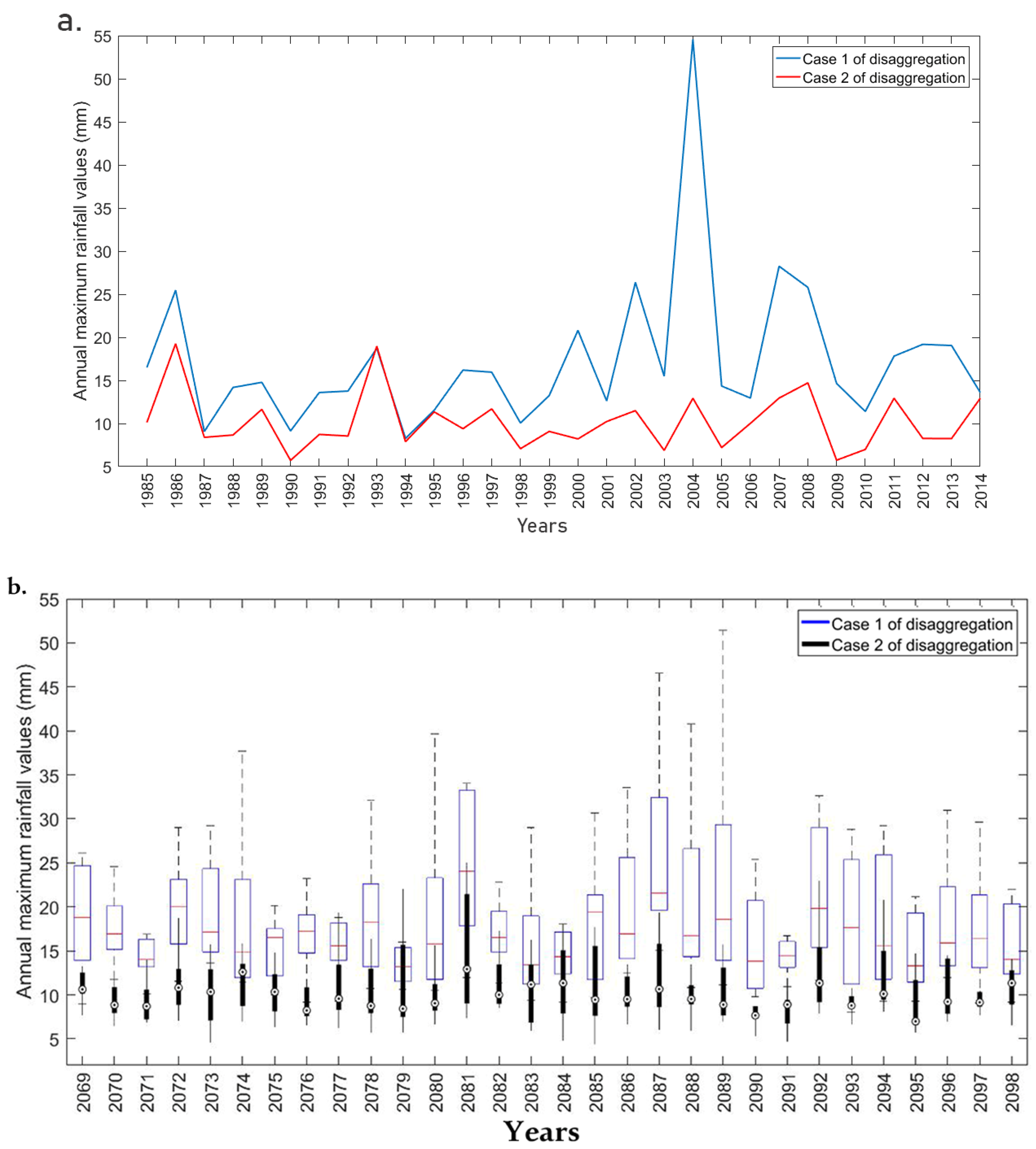
In order to make it easier for the reader to visualize the difference in AMs between the two cases of rainfall disaggregation, Figure 2a,b shows an example of the AM values for the disaggregated daily rainfall and for the current and future climates with a duration of 1 h. The future modeled rainfall data in Figure 2b and the above three examples were bias corrected based on the last reference period.
3.2. IDF Curves
The IDF curves for the current and future climates were derived for a small urban area in West Yorkshire by using the following: 11 RCM ensemble members, 5 rainfall durations, 6 return periods, 8 reference periods to bias correct the RCM, and 2 cases for rainfall disaggregation using the rainfall variable with and without the temperature variable. Then, the IDF curves were used to determine the percentage of relative change between the current and future climate. In addition, the uncertainty (which is the range of the results) of the future climate outputs was investigated by comparing 16 sets of future IDF curves. These sets were derived based on two cases of rainfall disaggregation and on the eight reference periods that were adopted to bias correct the future RCM rainfall data.
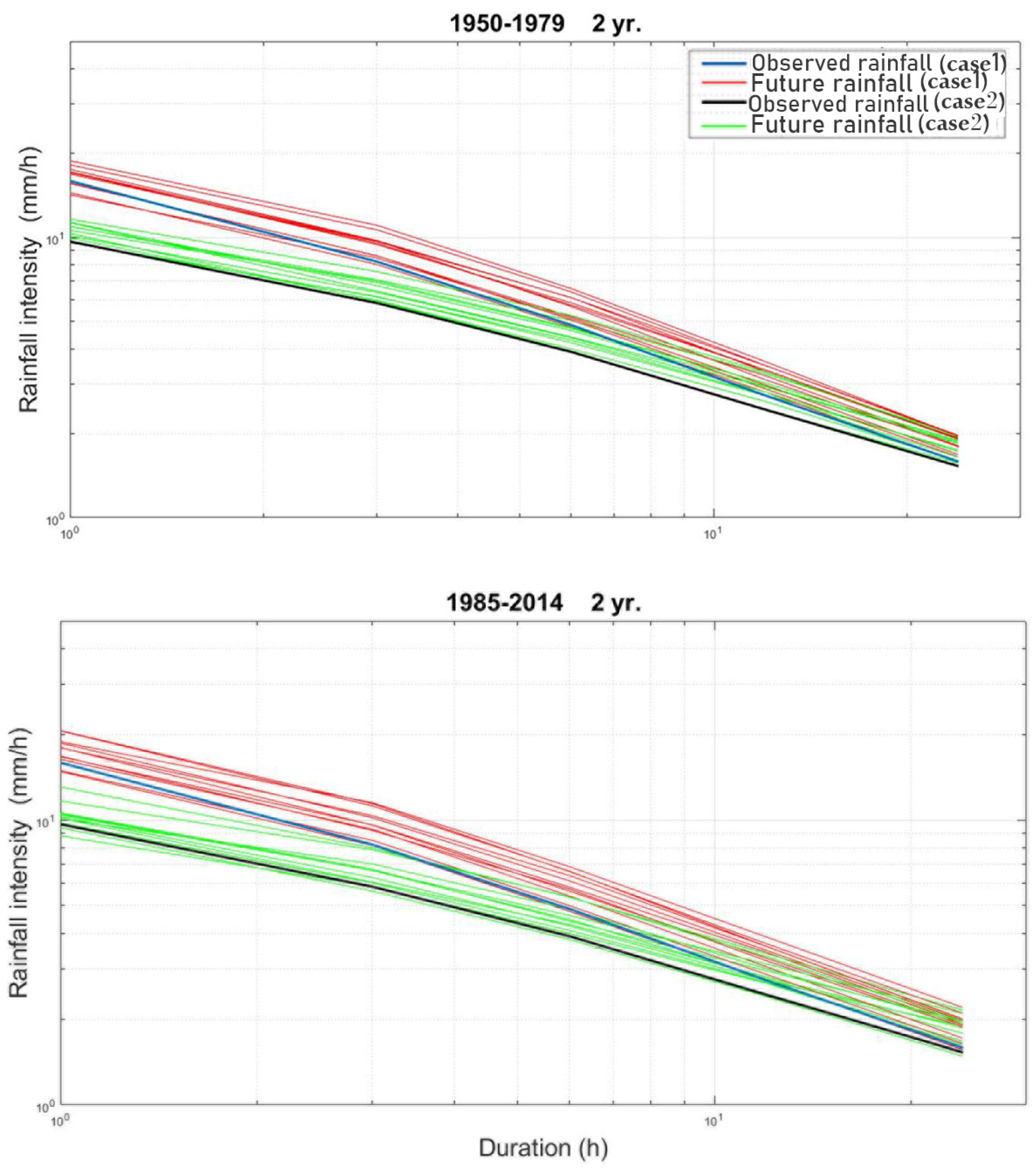
An example of the difference in IDF curves for both the current and future climate is presented in Figure 3 for the first and last reference periods and the two cases of rainfall disaggregation. The plots in the figure show that the future IDF curves differ from those of the current climate and the extent of the difference between them arises from the reference period (as previously stated by Fadhel et al. [38]), and also from the rainfall disaggregation method (i.e., the use or otherwise of the temperature variable together with the historical rainfall). In this study, the focus is not on the uncertainty that results from the reference period because this issue has already been addressed by Fathel et al. [38]. Instead, this study is interested in the uncertainty that may result from the rainfall disaggregation, where again this does not mean the uncertainty that results from the type of disaggregation method, but rather from the number of climate variables that are used for the disaggregation.
It is clear from Figure 3 (and Figures S1–S5 in the Supplementary Material and from the rest of the figures for the reference periods and rainfall disaggregation cases that are not shown here) that the projected rainfall intensity for most of the RCM ensemble members tends to increase for all frequencies, durations, reference periods, and rainfall disaggregation when case 2 is applied (i.e., without using the temperature variable). However, the results for future rainfall intensity, when also including the temperature variable in the rainfall disaggregation procedure (i.e., case 1), are similar to those of case 2 for all frequencies and durations except the first duration (i.e., 1 h) where the first five reference periods tend to project a decrease in the future rainfall intensity starting from the second return period (i.e., 5 years). Such a decrease in the projected rainfall intensity for the first duration is later shown by all the reference periods for the last three return periods (i.e., 25, 50, and 100 years) and by most of the climate ensemble members.
An interesting finding in respect of the results for the derived IDF curves was that the rainfall intensity for both the current and future climate which resulted from applying case 1 rainfall disaggregation (i.e., with temperature) was higher than that produced by case 2. This difference was seen for all reference periods, frequencies, and durations. As stated earlier in the Introduction, Wasko and Sharma [44] and Fadhel et al. [45] showed that in addition to the scaling of rainfall volume with temperature, each segment of the rainfall temporal pattern scales differently with temperature, especially the peak segment which scales positively with temperature. Consequently, the rainfall temporal pattern for the disaggregated rainfall based on the temperature and rainfall variables highly differs from that based on the rainfall variable alone, especially for the future climate scenarios because the weather is becoming warmer. Thus, disaggregating the rainfall based on case 2 (i.e., without temperature) can lead to a high over-under estimation of the actual results and uncertain outputs in regard to the derived IDF curves for both the current and future climate. It is also worth mentioning that the maximum likelihood estimate method was adopted to check the significance of the results at the 95% level and was applied to the parameters used for deriving the IDF curves (results not shown).
In this study, for each of the two cases of rainfall disaggregation, the percentage change between the future and current climate for the mean of the 11 RCM ensemble members was found in order to investigate the difference between the two climates and then compare the results of the two cases of rainfall disaggregation. A sample of the results is shown in Table 1 for 5 rainfall durations, the 2 cases of rainfall disaggregation, 8 reference periods, and the 10-year return period.
It is clear from Table 1 and the rest of the unshown results that by adopting the temperature variable to disaggregate the rainfall, the percentage change between the two climates was lower than the corresponding values for the case of disaggregation based on only the rainfall variable even though the rainfall values for both the current and future climates generated by the case 1 disaggregation method were higher than those obtained by applying case 2. This was true for all reference periods, durations, and frequencies with a few exceptions, vice versa. Such exceptions included (a) the first return period (2 years) for the first duration (1 h) and the last three reference periods; (b) the first return period for the second to the fourth durations (3 to 12 h) and all reference periods, and (c) the third duration (6 h) for all return periods and the last reference period.
However, the percentage change between the future and current climate for case 1 disaggregation and the first duration (i.e., 1 h) tended to indicate a projected decrease in the future rainfall intensity compared to the current climate for all return periods except for the first return period. Such a decrease in the projected rainfall intensity for the first duration was shown by five reference periods for the second return period (i.e., 5 years), and later expanded to include all eight reference periods for the last three return periods (i.e., 25, 50 and 100).
On the other hand, for the third return period (i.e., 10 years), only the seventh reference period showed a slight increase in future rainfall intensity compared to the current climate with a value of 0.64%, as shown in Table 1. By comparing the percentage change (i.e., for the seventh reference period, 1 h duration, and 10-year return period) by case 1 with that of case 2, it can be seen that the percentage change by case 1 was much lower than that by case 2 (i.e., 0.64% vs. 22.4%). Thus, the difference between the two values of percentage change for the two cases of rainfall disaggregation was 21.8%.
Staying with the same duration and return period (i.e., 1 h, 10 years) for case 1 rainfall disaggregation, the first reference period showed the maximum decrease in terms of the percentage change between the two climates with a value of −14.7%. However, the corresponding value for case 2 rainfall disaggregation in the first reference period showed an increase of 14.6%. Hence the difference between the predictions of the two cases is 29.3%. As can be seen from Table 1 (and the unshown results), the difference in the percentage change value between the two cases of disaggregation was higher for shorter durations and decreased as the duration increased for each return period.
As such differences in the percentage change values between the two cases of rainfall disaggregation were large compared with the return period and rainfall duration, the effect of the return period and rainfall duration on the percentage change between the current and future climate over the eight reference periods was investigated further for each case of rainfall disaggregation. Hence, the uncertainty in the difference between the results produced by the two cases of disaggregation were inspected as well.
It was found that the results (i.e., uncertainty in the difference in the percentage change between the two cases of rainfall disaggregation) varied over the eight reference periods. For each rainfall duration, the uncertainty of the results tended to increase as the return period increased. However, for each return period, the uncertainty in the difference of the projections between the two cases of rainfall disaggregation reduced as the rainfall duration increased over the eight reference periods. This was observed for all return periods except the first one (2 years) where the uncertainty declined for the first two durations (1 and 3 h) and increases for the last three (6, 12, and 24 h).
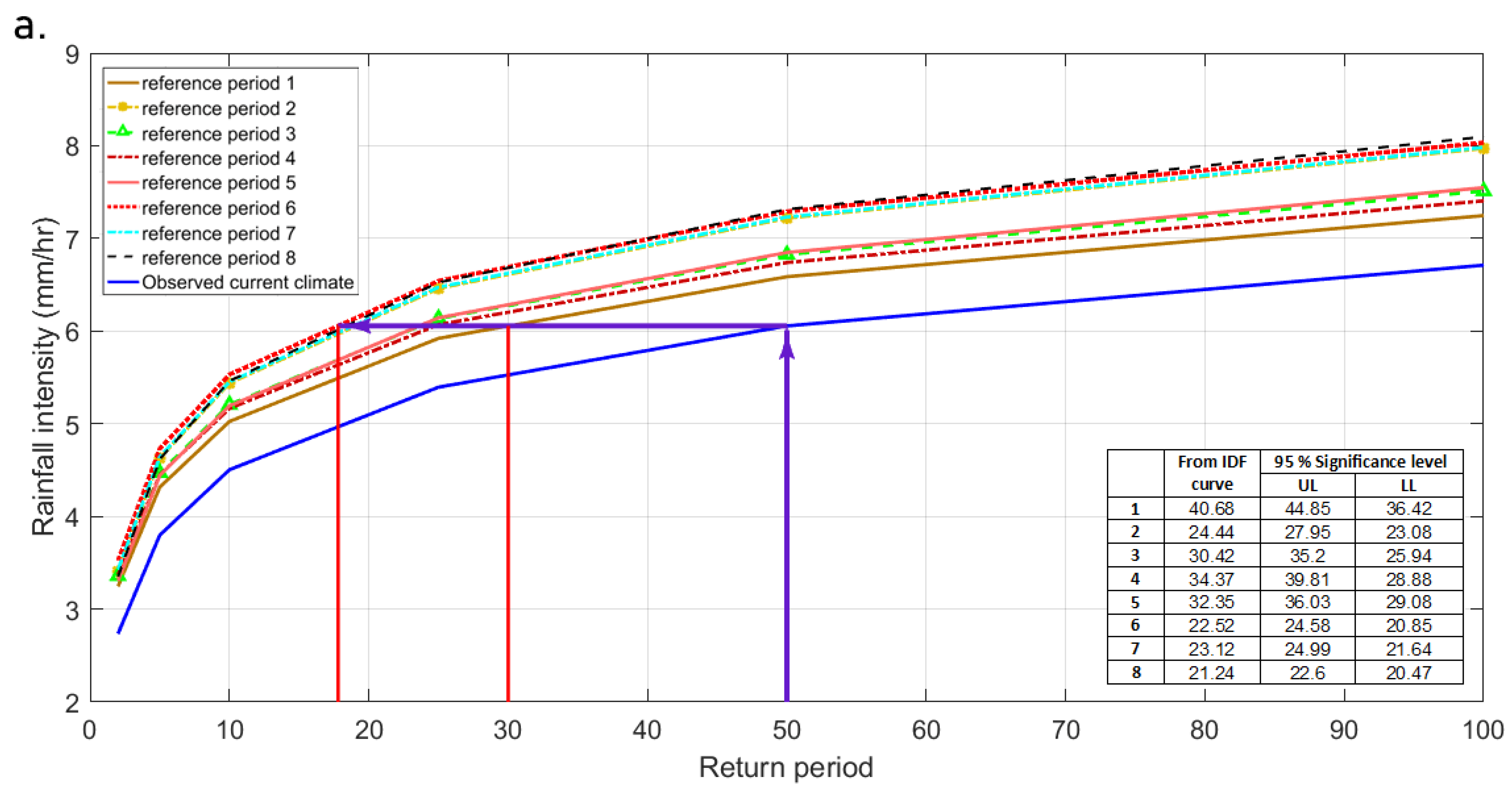
Since the projection results based on the two cases of rainfall disaggregation were not consistent for shorter durations and longer return periods, the results for all durations and return periods were examined in more detail. Figure 4 and Figure 5 show an example of the analysis of a short and a long duration of 3 h and 12 h, respectively, where both the current and future climates were plotted for the 8 reference periods, different return periods, the mean of the 11 RCM ensemble members, and the 2 cases of rainfall disaggregation.
It is clear from the graphs in Figure 4a,b and for a duration of 3 h, that for a specific rainfall intensity under the current climate that happened once every 50 years, the probability of such a specific rainfall occurring in any year was p = 2%. For the same rainfall intensity, but under future climate conditions and for case 1 rainfall disaggregation, the return period was found to vary between 21.2 and 40.7 years (i.e., p = 4.7–2.5%) based on the eight reference periods (Figure 4a). However, for case 2 rainfall disaggregation, the return period was found to be earlier than that for case 1 and it varied between 10.2 and 16.4 years (i.e., p = 9.8–6.1%) (Figure 4b). This means that the difference between the two ranges of the return period for the future climate depending on the two cases of rainfall disaggregation was between 11 and 24.3 years. When the above analysis was repeated for the duration of 12 h, it was noticed that the uncertainty varied between 17.8 and 30 years (Figure 5a) and between 9.9 and 16.9 years (Figure 5b) for case 1 and case 2, respectively. Thus, the difference between the two ranges for the two cases of disaggregation varied between 7.9 and 13.1 years. The above results were significant at the 95% level and are shown in a table within Figure 4 and Figure 5.
It is clear from the above analysis (and the unshown results) that the extent of uncertainty regarding a specific rainfall intensity under the current climate that is expected to appear in the future but with a shorter return period varies according to the case of disaggregation over the reference periods. In other words, the extent of uncertainty varies according to the climate variables that are used as predictors for the disaggregation. Such uncertainty is higher when the historical temperature and rainfall variables are adopted as predictors to disaggregate the rainfall as compared to using only the rainfall variable for disaggregation, and moreover, the uncertainty is significant for shorter durations and longer return periods. In addition, the difference between the results of the two cases of rainfall disaggregation is considerable for short durations and longer return periods.
Usually, global climate models and RCMs employ ensemble members to mitigate the uncertainty of future climate projections. The remainder of this section focuses on the uncertainty of future rainfall projections for 3 out of the 11 climate ensemble members: (1) the driest ensemble member; (2) the wettest ensemble member, and (3) the mean of the 11 RCM ensemble members. Table 2 presents a sample of the results of the projected rainfall intensity for future climate for the 10-year return period, 5 rainfall durations, 8 reference periods, and the 2 cases of rainfall disaggregation for the driest ensemble member, wettest ensemble member, and the mean of the 11 RCM ensemble members.
The wettest ensemble member is also known as the “pessimistic” climate scenario [11] since it gives the highest projection compared to the other climate ensemble members. In this study, it was found that the uncertainty related to the difference between the projected results based on the two cases of rainfall disaggregation and for all the reference periods increased as the return period increased for a specific rainfall duration. This uncertainty was considerable for small rainfall durations, especially the first two durations, but it tended to become less pronounced for rainfall durations higher than 6 h as the return period increased. However, the uncertainty of the future rainfall intensity that resulted from the difference between the two cases used to disaggregate the rainfall tended to decrease as the rainfall duration lengthened for a specific return period.
Similarly, the uncertainty for the driest ensemble member and the mean of the 11 RCM ensemble members increased for short rainfall durations and long return periods. Nevertheless, the extent of uncertainty was much lower than that for the wettest ensemble member.
As mentioned earlier, and as seen from Table 2 as well as the unshown results, the rainfall projections based on disaggregation by using both the temperature and the rainfall variables (case 1) were higher than the corresponding projections based on disaggregation by the rainfall variable alone (case 2). This was true for all reference periods, frequencies, and durations except for the last duration (24 h). For the 24 h duration, only the projections for a few climate ensemble members based on case 1 rainfall disaggregation were lower than the corresponding results based on case 2 rainfall disaggregation. However, the difference between these results for the two cases were very small because the predictions of the future rainfall intensity based on the two cases of rainfall disaggregation tended to be close to each other for the long durations and especially for the longest duration (i.e., 24 h).
4. Conclusions
In this study, a set of IDF curves for the current and future climate scenarios was derived and compared. Two cases of rainfall disaggregation were used to disaggregate the daily rainfall for both climates (i.e., current and future) to an hourly scale. One case was based on two climate variables, namely, historical temperature and historical rainfall, which were used as the predictors for the disaggregation (case 1). The other case was based on one climate variable only, i.e., historical rainfall (case 2). The uncertainty in the difference between the IDF curves which resulted from the two cases of disaggregation was assessed over eight reference periods. Each of the eight reference periods had a specified length of 30 years and a window of 5 years moving from the first to the last period. These reference periods were used to bias correct the future RCM rainfall data.
The projected results of the climate model based on the above two cases of rainfall disaggregation indicated that the percentage change between the projected and current rainfall intensities was significant. However, the uncertainty in the difference of percentage change between the two cases of disaggregation was found to vary with return period and rainfall duration. For each rainfall duration, the extent of uncertainty grew as the return period lengthened. On the other hand, the uncertainty decreased in each return period as the rainfall duration increased. However, the IDF curves that were produced on the basis of the two cases of disaggregation showed an increase in future rainfall projections as compared with the IDF curves of the current climate for all durations, frequencies, and over all eight reference periods, except for the first duration for case 1 disaggregation, which showed opposite results (i.e., a decline) in the future projection for all frequencies except the first frequency and by most of the reference periods. However, the projected and current rainfall values based on case 1 disaggregation were higher than the corresponding projections and current values based on case 2 disaggregation.
The return period for a specific rainfall intensity in the current climate is expected to be shorter when it appears in the future. The difference of the results for such a return period based on the two cases of rainfall disaggregation was found to be considerable. This difference was accompanied by high uncertainty over the eight reference periods and it became higher as the rainfall duration shortened and the return period lengthened. Moreover, the value of future rainfall intensity for the driest ensemble member, wettest ensemble member, and the mean of 11 RCM ensemble members was found to vary between the two cases of disaggregation and across the eight reference periods. The uncertainty related to this point is significant, especially for short rainfall durations and long return periods.
Overall, it can be clearly seen from the results of this study that the uncertainty in the projected IDF curves for the future climate is produced whether or not another climate variable (i.e., temperature) is adopted alongside historical rainfall as a predictor for rainfall disaggregation. Moreover, the effect of using temperature and rainfall instead of rainfall alone for the disaggregation of rainfall data from a daily to an hourly scale and, consequently, on the projection of future climate is significant. Due to climate change, the temperature rise and previous studies find that not just the rainfall volume scale with temperature. However, each fraction within the rainfall temporal pattern scales differently with temperature. So, the peak rainfall fraction scales positively with temperature and becomes peakier, while the non-peak fraction scales negatively with temperature and becomes less. Such a change in the rainfall temporal pattern would definitely have an effect on the peak flow of a sewer system and may lead to flooding. Thus, using both the temperature variable and the rainfall variable for disaggregation will produce accurate results for both AMs and storm profiles. Such AMs can be used to construct IDF curves while the storm profiles can be used to simulate design floods either by the continuous simulation or design storm approach.
While the above results are important for the engineering community, further research is required to examine some questions that remain unanswered. For example, how would the use of more than two climate variables (i.e., besides temperature and rainfall) for rainfall disaggregation affect the future IDF curves? Moreover, how would applying the results of the projected IDF curves for the two cases of rainfall disaggregation in a hydrological model affect the peak flow? Finally, how can the uncertainty of the peak flow be in comparison with the uncertainty of IDF curves? It is hoped that this study will motivate the research community to further investigate such questions.
Supplementary Materials
The following are available online at https://www.mdpi.com/article/10.3390/w13172337/s1, Figure S1. IDF curves for the current and future climate based on the two cases of rainfall disaggregation for the first and last reference periods. Each subplot is for the second return period and for five rainfall durations., Figure S2. IDF curves for the current and future climate based on the two cases of rainfall disaggregation for the first and last reference periods. Each subplot is for the third return period and for five rainfall durations., Figure S3. IDF curves for the current and future climate based on the two cases of rainfall disaggregation for the first and last reference periods. Each subplot is for the fourth return period and for five rainfall durations., Figure S4. IDF curves for the current and future climate based on the two cases of rainfall disaggregation for the first and last reference periods. Each subplot is for the fifth return period and for five rainfall durations., Figure S5. IDF curves for the current and future climate based on the two cases of rainfall disaggregation for the first and last reference periods. Each subplot is for the sixth return period and for five rainfall durations.
Author Contributions
Conceptualization, S.F.; methodology, S.F. and M.A.A.; software, S.F.; validation, M.S.S. and M.A.A.; formal analysis, S.F. and M.S.S.; writing—original draft preparation, M.S.S. and S.F.; writing—review and editing, M.A.A.; supervision, S.F. and M.A.A. All authors have read and agreed to the published version of the manuscript.
Funding
This research received no external funding.
Data Availability Statement
Not applicable.
Acknowledgments
The authors thank the UK Met Office, the Environment Agency, and the British Atmospheric Data Centre for providing the radar dataset. We also thank the Center of Ecology and Hydrology CEH for providing: The Gridded Estimates of Areal Rainfall (CEH_GEAR) dataset, the gridded temperature data through (CHESS-met) dataset, and the modeled climate data at 1 km within the urban area.
Conflicts of Interest
The authors declare no conflict of interest.
References
- Al Mamoon, A.; Joergensen, N.E.; Rahman, A.; Qasem, H. Design rainfall in Qatar: Sensitivity to climate change scenarios. Nat. Hazards 2016, 81, 1797–1810. [Google Scholar] [CrossRef]
- Aldosari, D.; Almedeij, J.; Alsumaiei, A.A. Update of intensity–duration–frequency curves for Kuwait due to extreme flash floods. Environ. Ecol. Stat. 2020, 27, 491–507. [Google Scholar] [CrossRef]
- Hosseinzadehtalaei, P.; Tabari, H.; Willems, P. Climate change impact on short-duration extreme precipitation and intensity–duration–frequency curves over Europe. J. Hydrol. 2020, 590, 125249. [Google Scholar] [CrossRef]
- Rodríguez, R.; Navarro, X.; Casas, M.C.; Ribalaygua, J.; Russo, B.; Pouget, L.; Redaño, A. Influence of climate change on IDF curves for the metropolitan area of Barcelona (Spain). Int. J. Climatol. 2014, 34, 643–654. [Google Scholar] [CrossRef] [Green Version]
- Zhao, W.; Kinouchi, T.; Nguyen, H.Q. A framework for projecting future intensity-duration-frequency (IDF) curves based on CORDEX Southeast Asia multi-model simulations: An application for two cities in Southern Vietnam. J. Hydrol. 2021, 598, 126461. [Google Scholar] [CrossRef]
- Dahm, R.; Bhardwaj, A.; Weiland, F.S.; Corzo, G.; Bouwer, L.M. A temperature-scaling approach for projecting changes in short duration rainfall extremes from GCM data. Water 2019, 11, 313. [Google Scholar] [CrossRef] [Green Version]
- Mailhot, A.; Duchesne, S. Design Criteria of Urban Drainage Infrastructures under Climate Change. J. Water Resour. Plan. Manag. 2010, 136, 201–208. [Google Scholar] [CrossRef]
- Silva, D.F.; Simonovic, S.P.; Schardong, A.; Goldenfum, J.A. Introducing non-stationarity into the development of intensity-duration-frequency curves under a changing climate. Water 2021, 13, 1008. [Google Scholar] [CrossRef]
- Intergovernmental Panel on Climate Change (IPCC). Managing the risks of extreme events and disasters to advance climate change adaptation. In Special Report of Working Groups I and II of the Intergovernmental Panel on Climate Change; Field, C.B., Barros, V., Stocker, T.F., Qin, D., Dokken, D.J., Ebi, K.L., Mastrandrea, M.D., Mach, K.J., Plattner, G.K., Allen, S.K., et al., Eds.; Cambridge University Press: New York, NY, USA, 2012. [Google Scholar]
- Intergovernmental Panel on Climate Change (IPCC). Climate Change 2013: The Physical Science Basis. In Contribution of Working Group I to the Fifth Assessment Report of the Intergovernmental Panel on Climate Change; Stocker, T.F., Qin, D., Plattner, G.K., Tignor, M., Allen, S.K., Boschung, J., Nauels, A., Xia, Y., Bex, V., Midgley, P.M., et al., Eds.; Cambridge University Press: Cambridge, UK; New York, NY, USA, 2013; p. 1535. [Google Scholar]
- Willems, P. Revision of urban drainage design rules after assessment of climate change impacts on precipitation extremes at Uccle, Belgium. J. Hydrol. 2013, 496, 166–177. [Google Scholar] [CrossRef]
- Watt, E.; Marsalek, J. Critical review of the evolution of the design storm event concept. Can. J. Civ. Eng. 2013, 40, 105–113. [Google Scholar] [CrossRef]
- Segond, M.-L.; Onof, C.; Wheater, H.S. Spatial-temporal disaggregation of daily rainfall from a generalized linear model. J. Hydrol. 2006, 331, 674–689. [Google Scholar] [CrossRef]
- Watt, W.E.; Waters, D.; McLean, R. Climate Variability and Urban Stormwater Infrastructure in Canada: Context and Case Studies; Toronto-Niagara Region Study Report and Working Paper Series, Report 2003-1; Meteorological Service of Canada: Waterloo, ON, Canada, 2003.
- Cowpertwait, P.S. Further developments of the Neyman–Scott clustered point process for modeling rainfall. Water Resour. Res. 1991, 27, 1431–1438. [Google Scholar] [CrossRef]
- Kim, D.; Kwon, H.-H.; Lee, S.-O.; Kim, S. Regionalization of the modified Bartlett–Lewis rectangular pulse stochastic rainfall model across the Korean peninsula. J. Hydro-Environ. Res. 2016, 11, 123–137. [Google Scholar] [CrossRef]
- Rodriguez-Iturbe, I.; Cox, D.R.; Isham, V. Some models for precipitation based on stochastic point processes. Proc. R. Soc. London Ser. A 1987, 410, 269–288. [Google Scholar] [CrossRef]
- De Luca, D.L.; Petroselli, A. STORAGE (STOchastic RAinfall GEnerator): A user-friendly software for generating long and high-resolution rainfall time series. Hydrology 2021, 8, 76. [Google Scholar] [CrossRef]
- De Luca, D.L.; Petroselli, A.; Galasso, L. A transient stochastic rainfall generator for climate changes analysis at hydrological scales in Central Italy. Atmosphere 2020, 11, 1292. [Google Scholar] [CrossRef]
- Chandler, R.E.; Wheater, H.S. Analysis of precipitation variability using generalized linear models: A case study from the west of Ireland. Water Resour. Res. 2002, 38, 1192. [Google Scholar] [CrossRef] [Green Version]
- Cârsteanu, A.; Foufoula-Georgiou, E. Assessing dependence among weights in a multiplicative cascade model of temporal rainfall. J. Geophys. Res. 1996, 101, 26363–26370. [Google Scholar] [CrossRef]
- Gupta, V.K.; Waymire, E.C. A statistical analysis of mesoscale rainfall as a random cascade. J. Appl. Meteorol. 1993, 322, 251–267. [Google Scholar] [CrossRef]
- Muzy, J.F.; Baïle, R. Self-similar continuous cascades supported by random cantor sets: Application to rainfall data. Phys. Rev. E 2016, 93, 052305. [Google Scholar] [CrossRef] [Green Version]
- Rupp, D.E.; Keim, R.F.; Ossiander, M.; Brugnach, M.; Selker, J.S. Time scale and intensity dependency in multiplicative cascades for temporal rainfall disaggregation. Water Resour. Res. 2009, 45, W07409. [Google Scholar] [CrossRef] [Green Version]
- Burian, B.S.J.; Durrans, S.R.; Tomic, S.; Pimmel, R.L.; Wai, C.N. Rainfall disaggregation using Artificial Neural Networks. J. Hydrol. Eng. 2000, 5, 299–307. [Google Scholar] [CrossRef]
- Buishand, T.A.; Brandsma, T. Multisite simulation of daily precipitation and temperature in the Rhine basin by nearest-neighbor resampling. Water Resour. Res. 2001, 37, 2761–2776. [Google Scholar] [CrossRef]
- Lall, U.; Sharma, A. A nearest neighbor bootstrap for time series resampling. Water Resour. Res. 1996, 32, 679–693. [Google Scholar] [CrossRef]
- Sharif, M.; Burn, D.H. Improved K-nearest neighbor weather generating model. J. Hydrol. Eng. 2007, 12, 42–51. [Google Scholar] [CrossRef] [Green Version]
- Yates, D.; Gangopadhyay, S.; Rajagopalan, B.; Strzepek, K. A technique for generating regional climate scenarios using a nearest-neighbor algorithm. Water Resour. Res. 2003, 39, SWC7-1–SWC7-14. [Google Scholar] [CrossRef] [Green Version]
- Lu, Y.; Qin, X.S. Multisite precipitation downscaling and disaggregation in a tropical urban area. J. Hydrol. 2014, 509, 55–65. [Google Scholar] [CrossRef]
- Sharma, A.; Srikanthan, S. Continuous rainfall simulation: A nonparametric alternative. In 30th Hydrology and Water Resources Symposium: Past, Present & Future; Conference Design: Tasmania, Australia, 2006; p. 86. [Google Scholar]
- Srikanthan, R.; McMahon, T.A. Stochastic Generation of Rainfall and Evaporation Data; Technical Report 84; Australian Water Resources Council, Department of Resources and Energy: Canberra, Australia, 1985. [Google Scholar]
- Westra, S.; Mehrotra, R.; Sharma, A.; Srikanthan, R. Continuous rainfall simulation: 1. A regionalized subdaily disaggregation approach. Water Resour. Res. 2012, 48. [Google Scholar] [CrossRef] [Green Version]
- Choi, J.; Socolofsky, S.A.; Olivera, F. Hourly disaggregation of daily rainfall in Texas using measured hourly precipitation at other locations. J. Hydrol. Eng. 2008, 13, 476–487. [Google Scholar] [CrossRef] [Green Version]
- Li, X.; Meshgi, A.; Wang, X.; Zhang, J.; Tay, S.H.X.; Pijcke, G.; Manocha, N.; Ong, M.; Nguyen, M.T.; Babovic, V. Three resampling approaches based on method of fragments for daily-to-subdaily precipitation disaggregation. Int. J. Clim. 2018, 38, e1119–e1138. [Google Scholar] [CrossRef]
- Pampaloni, M.; Sordo-Ward, A.; Bianucci, P.; Martin, I.G.; Caporali, E.; Garrote, L. A stochastic procedure for temporal disaggregation of daily rainfall data in SuDS design. Water 2021, 13, 403. [Google Scholar] [CrossRef]
- Pui, A.; Sharma, A.; Mehrotra, R.; Sivakumar, B.; Jeremiah, E. A comparison of alternatives for daily to sub-daily rainfall disaggregation. J. Hydrol. 2012, 470–471. [Google Scholar] [CrossRef] [Green Version]
- Fadhel, S.; Rico-Ramirez, M.A.; Han, D. Uncertainty of Intensity-Duration-Frequency (IDF) curves due to varied climate baseline periods. J. Hydrol. 2017, 547, 600–612. [Google Scholar] [CrossRef] [Green Version]
- Westra, S.; Evans, J.P.; Mehrotra, R.; Sharma, A. A conditional disaggregation algorithm for generating fine time-scale rainfall data in a warmer climate. J. Hydrol. 2013, 479, 86–99. [Google Scholar] [CrossRef] [Green Version]
- Yang, Q.; Dai, Q.; Han, D.; Zhu, X.; Zhang, S. An uncertainty investigation of RCM downscaling ratios in nonstationary extreme rainfall IDF curves. Atmosphere 2018, 9, 151. [Google Scholar] [CrossRef] [Green Version]
- Alam, M.S.; Elshorbagy, A. Quantification of the climate change-induced variations in Intensity-Duration-Frequency curves in the Canadian Prairies. J. Hydrol. 2015, 527, 990–1005. [Google Scholar] [CrossRef]
- Uraba, M.B.; Gunawardhana, L.N.; Al-Rawas, G.A.; Baawai, M.S. A downscaling-disaggregation approach for developing IDF curves in arid regions. Environ. Monit. Assess. 2019, 191, 245. [Google Scholar] [CrossRef] [PubMed]
- Butler, D.; Digman, C.J.; Makropoulos, C.; Davies, J.W. Urban Drainage, 4th ed.; CRC Press: Boca Raton, FL, USA, 2018. [Google Scholar]
- Wasko, C.; Sharma, A. Steeper temporal distribution of rain intensity at higher temperatures within Australian storms. Nat. Geosci. 2015, 8, 527–529. [Google Scholar] [CrossRef]
- Fadhel, S.; Rico-Ramirez, M.A.; Han, D. Sensitivity of peak flow to the change of rainfall temporal pattern due to climate change. J. Hydrol. 2018, 560, 546–559. [Google Scholar] [CrossRef] [Green Version]
- Keller, V.D.J.; Tanguy, M.; Prosdocimi, I.; Terry, J.A.; Hitt, O.; Cole, S.J.; Fry, M.; Morris, D.G.; Dixon, H. CEH-GEAR: 1 km resolution daily and monthly areal rainfall estimates for the UK for hydrological and other applications. Earth Syst. Sci. Data 2015, 7, 143–155. [Google Scholar] [CrossRef] [Green Version]
- Perry, M.; Hollis, D. The generation of monthly gridded datasets for a range of climatic variables over the UK. Int. J. Climatol. 2005, 25, 1041–1054. [Google Scholar] [CrossRef]
- Eden, P. Traditional weather observing in the UK: An historical overview. Weather 2009, 64, 239–245. [Google Scholar] [CrossRef]
- Met Office, U.K. Fact Sheet No. 15—Weather Radar. 2009. Available online: http://www.metoffice.gov.uk/learning/library/factsheets (accessed on 12 May 2014).
- Harrison, D.L.; Scovell, R.W.; Kitchen, M. High-resolution precipitation estimates for hydrological uses. Proc. Inst. Civ. Eng-Water Manag. 2009, 162, 125–135. [Google Scholar] [CrossRef]
- Fadhel, S.; Rico-Ramirez, M.A.; Han, D. Exploration of an adaptive merging scheme for optimal. J. Hydroinform. 2017, 19, 225–237. [Google Scholar] [CrossRef] [Green Version]
- Robinson, E.L.; Blyth, E.; Clark, D.B.; Comyn-Platt, E.; Finch, J.; Rudd, A.C. Climate Hydrology and Ecology Research Support System Meteorology Dataset for Great Britain (1961–2015) [CHESS-met]. NERC Environmental Information Data Centre. Available online: https://doi.org/10.5285/b745e7b1-626c-4ccc-ac27-56582e77b900 (accessed on 10 January 2017).
- Murphy, J.M.; Sexton, D.M.H.; Jenkins, G.J.; Booth, B.B.B.; Brown, C.C.; Clark, R.T.; Collins, M.; Harris, G.R.; Kendon, E.J.; Betts, R.A.; et al. UK Climate Projections Science Report: Climate Change Projections; Met Office Hadley Centre: Exeter, UK, 2009; p. 190. [Google Scholar]
- Newton, G.; Dadson, S.J.; Lafon, T.; Prudhomme, C. Scoping Study for Precipitation Downscaling and Bias-Correctio—Science Report/Project Note SC090016/PN3; CEH: Wallingford, UK, 2012; p. 41. Available online: http://nora.nerc.ac.uk/id/eprint/15043 (accessed on 19 August 2021).
- Prudhomme, C.; Dadson, S.; Morris, D.; Williamson, J.; Goodsell, G.; Crooks, S.; Watts, G. Future Flows Climate: An ensemble of 1-km climate change projections for hydrological application in Great Britain. Earth Syst. Sci. Data 2012, 4, 143–148. [Google Scholar] [CrossRef] [Green Version]
- Yang, W.; Andreasson, J.; Graham, L.P.; Olsson, J.; Rosberg, J.; Wetterhall, F. Distribution-based scaling to improve usability of regional climate model projections for hydrological climate change impacts studies. Hydrol. Res. 2010, 41, 211–229. [Google Scholar] [CrossRef]
- Olsson, T.; Jakkila, J.; Veijalainen, N.; Backman, L.; Kaurola, J.; Vehvilainen, B. Impacts of climate change on temperature, precipitation and hydrology in Finland—Studies using bias corrected Regional Climate Model data. Hydrol. Earth Syst. Sci. 2015, 19, 3217–3238. [Google Scholar] [CrossRef] [Green Version]
- Sharma, A.; Mehrotra, R.; Li, J.W.; Jha, S. A programming tool for nonparametric system prediction using Partial Informational Correlation and Partial Weights. Environ. Model. Softw. 2016, 83, 271–275. [Google Scholar] [CrossRef]
- Mehrotra, R.; Westra, S.; Sharma, A.; Srikanthan, R. Continuous rainfall simulation: 2. A regionalized daily rainfall generation approach. Water Resour. Res. 2012, 48, 1536. [Google Scholar] [CrossRef] [Green Version]
- Millington, N.; Das, S.; Simonovic, S.P. The Comparison of GEV, Log-Pearson Type 3 and Gumbel Distributions in the Upper Thames River Watershed under Global Climate Models; Water Resources Research Report No. 077; Department of Civil and Environmental Engineering, University of Western Ontario London: London, ON, Canada, 2011; ISSN: 19133200; Available online: http://ir.lib.uwo.ca/wrrr/40 (accessed on 19 August 2021).
- Azizian, A. Uncertainty analysis of time of concentration equations based on first-order-analysis (FOA) method. Am. J. Eng. Appl. Sci. 2018, 11, 327–341. [Google Scholar] [CrossRef]
- Michailidi, E.M.; Antoniadi, S.; Koukouvinos, A.; Bacchi, B.; Efstratiadis, A. Timing the time of concentration: Shedding light on a paradox. Hydrol. Sci. 2018, 63, 721–740. [Google Scholar] [CrossRef] [Green Version]
- USDA, Natural Resources Conservation Service. National Engineering Handbook; Part 630; Chapter 15; Time of Concentration: Washington, DC, USA, 2010. [Google Scholar]
Figure 1.
Flowchart for the process of creating IDF curves.

Figure 2.
Annual maximum rainfall values produced by the 2 cases of rainfall disaggregation, for the current climate (a), and the future climate (b).
Figure 2.
Annual maximum rainfall values produced by the 2 cases of rainfall disaggregation, for the current climate (a), and the future climate (b).

Figure 3.
IDF curves for the current and future climate based on the 2 cases of rainfall disaggregation for the first and last reference periods. The two subplots are for the first return period and for 5 rainfall durations.
Figure 3.
IDF curves for the current and future climate based on the 2 cases of rainfall disaggregation for the first and last reference periods. The two subplots are for the first return period and for 5 rainfall durations.

Figure 4.
The rainfall intensity of current and future climates for 3 h duration and the 2 cases of disaggregation, case 1 (a), case 2 (b), and for different frequencies, and 8 reference periods.
Figure 4.
The rainfall intensity of current and future climates for 3 h duration and the 2 cases of disaggregation, case 1 (a), case 2 (b), and for different frequencies, and 8 reference periods.


Figure 5.
The rainfall intensity of current and future climates for 12 h duration and the 2 cases of disaggregation, case 1 (a), case 2 (b), and for different frequencies, and 8 reference periods.
Figure 5.
The rainfall intensity of current and future climates for 12 h duration and the 2 cases of disaggregation, case 1 (a), case 2 (b), and for different frequencies, and 8 reference periods.


Table 1.
The percentage change between the future and current climate for the mean of the 11 RCM ensemble members, 5 rainfall durations, 2 cases of rainfall disaggregation, 8 reference periods, and the 10-year return period.
Table 1.
The percentage change between the future and current climate for the mean of the 11 RCM ensemble members, 5 rainfall durations, 2 cases of rainfall disaggregation, 8 reference periods, and the 10-year return period.
| Reference Period | Case 1 of Disaggregation | Case 2 of Disaggregation | ||||||||
|---|---|---|---|---|---|---|---|---|---|---|
| 1 h | 3 h | 6 h | 12 h | 1 Day | 1 h | 3 h | 6 h | 12 h | 1 Day | |
| 1950–1979 | −14.71 | 6.96 | 11.05 | 11.58 | 12.58 | 14.60 | 19.60 | 21.61 | 21.64 | 15.67 |
| 1955–1984 | −9.09 | 14.78 | 19.22 | 20.73 | 21.38 | 22.12 | 28.81 | 31.89 | 31.85 | 24.51 |
| 1960–1989 | −8.06 | 11.95 | 15.70 | 15.59 | 17.26 | 18.99 | 23.56 | 22.68 | 22.36 | 19.39 |
| 1965–1994 | −8.71 | 10.52 | 14.57 | 14.69 | 16.34 | 19.20 | 22.06 | 21.43 | 21.57 | 19.07 |
| 1970–1999 | −7.20 | 10.39 | 14.80 | 15.31 | 17.34 | 15.39 | 19.93 | 22.46 | 23.26 | 20.13 |
| 1975–2004 | −0.27 | 17.46 | 21.01 | 22.81 | 22.75 | 22.99 | 26.54 | 28.13 | 27.77 | 27.02 |
| 1980–2009 | 0.65 | 16.54 | 20.53 | 21.06 | 22.19 | 22.43 | 23.36 | 21.93 | 24.55 | 25.77 |
| 1985–2014 | −1.46 | 18.35 | 21.40 | 21.26 | 23.29 | 24.67 | 22.03 | 18.18 | 21.85 | 26.27 |
Table 2.
The projected future rainfall intensity for 10-year return period, 5 rainfall durations, 8 reference periods, 2 cases of rainfall disaggregation, and for the driest ensemble member, wettest ensemble member, and the mean of the 11 RCM ensemble members.
Table 2.
The projected future rainfall intensity for 10-year return period, 5 rainfall durations, 8 reference periods, 2 cases of rainfall disaggregation, and for the driest ensemble member, wettest ensemble member, and the mean of the 11 RCM ensemble members.
| Wettest Ensemble Member | ||||||||||
| Reference Period | Case 1 of Disaggregation | Case 2 of Disaggregation | ||||||||
| 1 h | 3 h | 6 h | 12 h | 1 Day | 1 h | 3 h | 6 h | 12 h | 1 Day | |
| 1950–1979 | 31.93 | 18.25 | 10.65 | 5.81 | 3.14 | 19.69 | 12.08 | 8.65 | 5.42 | 3.11 |
| 1955–1984 | 35.18 | 20.12 | 12.04 | 6.40 | 3.50 | 21.81 | 12.96 | 9.85 | 6.07 | 3.43 |
| 1960–1989 | 37.98 | 18.33 | 11.12 | 5.96 | 3.32 | 21.68 | 12.97 | 8.85 | 5.54 | 3.24 |
| 1965–1994 | 36.10 | 17.44 | 10.67 | 5.90 | 3.30 | 21.74 | 13.11 | 8.78 | 5.51 | 3.23 |
| 1970–1999 | 36.21 | 20.69 | 11.75 | 6.51 | 3.59 | 22.56 | 14.56 | 10.03 | 5.95 | 3.58 |
| 1975–2004 | 42.11 | 20.74 | 12.33 | 6.61 | 3.63 | 23.53 | 14.14 | 9.81 | 5.96 | 3.63 |
| 1980–2009 | 46.58 | 22.99 | 13.67 | 7.53 | 4.22 | 23.22 | 13.56 | 9.16 | 6.46 | 4.20 |
| 1985–2014 | 39.36 | 21.98 | 12.91 | 7.01 | 3.87 | 25.46 | 14.16 | 9.05 | 5.49 | 3.85 |
| Driest Ensemble Member | ||||||||||
| Reference Period | Case 1 of Disaggregation | Case 2 of Disaggregation | ||||||||
| 1 h | 3 h | 6 h | 12 h | 1 Day | 1 h | 3 h | 6 h | 12 h | 1 Day | |
| 1950–1979 | 21.53 | 11.81 | 7.81 | 4.48 | 2.49 | 13.29 | 8.70 | 5.80 | 3.68 | 2.44 |
| 1955–1984 | 20.07 | 11.39 | 7.36 | 4.36 | 2.45 | 13.56 | 8.73 | 5.84 | 3.65 | 2.31 |
| 1960–1989 | 21.96 | 11.80 | 7.18 | 3.99 | 2.23 | 13.58 | 8.45 | 5.68 | 3.59 | 2.25 |
| 1965–1994 | 23.45 | 12.27 | 7.16 | 4.17 | 2.38 | 14.23 | 8.64 | 5.91 | 3.76 | 2.37 |
| 1970–1999 | 23.14 | 12.05 | 7.35 | 4.31 | 2.39 | 14.14 | 8.71 | 5.88 | 3.72 | 2.45 |
| 1975–2004 | 22.56 | 13.21 | 7.84 | 4.52 | 2.60 | 15.09 | 8.73 | 5.82 | 3.87 | 2.65 |
| 1980–2009 | 23.97 | 12.00 | 6.92 | 4.06 | 2.20 | 14.27 | 8.63 | 5.77 | 3.62 | 2.19 |
| 1985–2014 | 23.08 | 11.82 | 6.63 | 3.75 | 2.19 | 13.08 | 8.00 | 5.47 | 3.44 | 2.11 |
| Mean of Ensemble Members | ||||||||||
| Reference Period | Case 1 of Disaggregation | Case 2 of Disaggregation | ||||||||
| 1 h | 3 h | 6 h | 12 h | 1 Day | 1 h | 3 h | 6 h | 12 h | 1 Day | |
| 1950–1979 | 26.44 | 14.94 | 9.00 | 5.03 | 2.77 | 16.72 | 10.45 | 7.40 | 4.62 | 2.73 |
| 1955–1984 | 28.18 | 16.03 | 9.66 | 5.44 | 2.99 | 17.81 | 11.25 | 8.03 | 5.01 | 2.94 |
| 1960–1989 | 28.50 | 15.63 | 9.37 | 5.21 | 2.88 | 17.36 | 10.80 | 7.47 | 4.65 | 2.82 |
| 1965–1994 | 28.30 | 15.43 | 9.28 | 5.17 | 2.86 | 17.39 | 10.66 | 7.39 | 4.62 | 2.81 |
| 1970–1999 | 28.77 | 15.42 | 9.30 | 5.19 | 2.89 | 16.83 | 10.48 | 7.46 | 4.68 | 2.84 |
| 1975–2004 | 30.92 | 16.40 | 9.80 | 5.53 | 3.02 | 17.94 | 11.05 | 7.80 | 4.85 | 3.00 |
| 1980–2009 | 31.20 | 16.28 | 9.76 | 5.45 | 3.01 | 17.86 | 10.78 | 7.42 | 4.73 | 2.97 |
| 1985–2014 | 30.55 | 16.53 | 9.83 | 5.46 | 3.03 | 18.18 | 10.66 | 7.20 | 4.63 | 2.98 |
Publisher’s Note: MDPI stays neutral with regard to jurisdictional claims in published maps and institutional affiliations. |
© 2021 by the authors. Licensee MDPI, Basel, Switzerland. This article is an open access article distributed under the terms and conditions of the Creative Commons Attribution (CC BY) license (https://creativecommons.org/licenses/by/4.0/).
Share and Cite
MDPI and ACS Style
Fadhel, S.; Al Aukidy, M.; Saleh, M.S. Uncertainty of Intensity-Duration-Frequency Curves Due to Adoption or Otherwise of the Temperature Climate Variable in Rainfall Disaggregation. Water 2021, 13, 2337. https://doi.org/10.3390/w13172337
AMA Style
Fadhel S, Al Aukidy M, Saleh MS. Uncertainty of Intensity-Duration-Frequency Curves Due to Adoption or Otherwise of the Temperature Climate Variable in Rainfall Disaggregation. Water. 2021; 13(17):2337. https://doi.org/10.3390/w13172337
Chicago/Turabian StyleFadhel, Sherien, Mustafa Al Aukidy, and May Samir Saleh. 2021. "Uncertainty of Intensity-Duration-Frequency Curves Due to Adoption or Otherwise of the Temperature Climate Variable in Rainfall Disaggregation" Water 13, no. 17: 2337. https://doi.org/10.3390/w13172337
Note that from the first issue of 2016, this journal uses article numbers instead of page numbers. See further details here.