
A Systematic Analysis of the Interaction between Rain-on-Grid-Simulations and Spatial Resolution in 2D Hydrodynamic Modeling


Chair of Engineering Hydrology and Water Management, Technical University of Darmstadt, 64287 Darmstadt, Germany
*
Author to whom correspondence should be addressed.
Water 2021, 13(17), 2346; https://doi.org/10.3390/w13172346
Submission received: 4 August 2021
/
Revised: 19 August 2021
/
Accepted: 21 August 2021
/
Published: 26 August 2021
(This article belongs to the Section Hydrology)
Abstract
:A large number of 2D models were originally developed as 1D models for the calculation of water levels along the main course of a river. Due to their development as 2D distributed models, the majority have added precipitation as a source term. The models can now be used as quasi-2D hydrodynamic rainfall–runoff models (‘HDRRM’). Within the direct rainfall method (‘DRM’), there is an approach, referred to as ‘rain-on-grid’, in which input precipitation is applied to the entire catchment area. The study contains a systematic analysis of the model behavior of HEC-RAS (‘Hydrologic Engineering Center—River Analysis System’) with a special focus on spatial resolution. The rain-on-grid approach is applied in a small, ungauged, low-mountain-range study area (Messbach catchment, 2.13 km2) in Central Germany. Suitable model settings and recommendations on model discretization and parametrization are derived therefrom. The sensitivity analysis focuses on the influence of the mesh resolution’s interaction with the spatial resolution of the underlying terrain model (‘subgrid’). Furthermore, the sensitivity of the parameters interplaying with spatial resolution, like the height of the laminar depth, surface roughness, model specific filter-settings and the precipitation input-data temporal distribution, is analyzed. The results are evaluated against a high-resolution benchmark run, and further criteria, such as 1. Nash–Sutcliffe efficiency, 2. water-surface elevation, 3. flooded area, 4. volume deficit, 5. volume balance and 6. computational time. The investigation showed that, based on the chosen criteria for this size and type of catchment, a mesh resolution between 3 m to 5 m, in combination with a DEM resolution from 0.25 m to 1 m, are recommendable. Furthermore, we show considerable scale effects on flooded areas for coarser meshing, due to low water levels in relation to topographic height.
1. Introduction
Motivation and Research Gap
The use of 2D hydrodynamic models to determine storm hazards in rural and urban catchments based on the direct rainfall method (in the following, DRM or ‘rain-on -grid’, compare with Ball et al. 2012 [1]) has recently become state-of-the-art in storm hazard flood modeling. The DRM has, meanwhile, established itself and is included in the mainstream commercial and non-commercial 2D software packages for urban or river flooding. Examples of applications of DRM together with a hydrodynamic Rainfall–runoff Model (HDRRM) or “hydro-inundation model” [2] can be found for urban and rural areas in Zeiger & Hubbart, (2021) [3], Krvavica & Rubinić (2020) [4], David & Schmalz (2020) [5], Broich et al. (2019) [6], Jia et al. (2019) [7], Tyrna et al. (2018) [8], Yu et al. (2015) [2], Cea et al. (2010) [9] or Hunter et al. (2008) [10].
The models for fluvial flood hazard assessment were often originally designed as 1D models to determine the water levels and floodplains along the 1D river stream. With the increased availability of high-resolution data of the terrain (‘digital elevation model’, DEM) and the surface (‘digital surface model’) these models also increased their level of detail, with their extension from 1D to 2D [11]. With this extension, floodplains and backwater effects are also modeled in high resolution. Due to the simultaneous increase of flood events—apart from large rivers (urban, pluvial or flash floods [12])—these 2D models were expanded to include the source terms of precipitation. This enables the models to be used in the context of storm-hazard analysis within an entire catchment area [5].
The problem of the application of 2D hydrodynamic models for the use of catchment hydrology and the determination of shallow overland flow is that the model is applied in ways for which it was not originally developed. However, the flow behavior of the thin-layer runoff differs greatly from the flow process in a ‘normal’ river, due to the very low flow depths [13,14]. The model user must consider this different way of application and need to take care of a suitable model parametrization. During the process of model creation, details such as spatial resolution, computational settings or roughness values have to be determined by the user. These should be suitable, on the one hand, to best represent the characteristics of the catchment, but on the other hand, also need to consider the special type of application of direct precipitation. It can be seen, for example, in Broich et al. (2019) [6] or in David & Schmalz (2020) [5] that with the use of a 2D model, such as 2D HDRRM, the model shows different behavior than for fluvial flood-hazard assessment. Other model settings are required for this application, and model parameters that were so far ignored may be sensitive. For this reason, before using the DRM in combination with a 2D model, the model should first be evaluated extensively with regard to its modelled behavior in relation to the parameterization and parameter’s sensitivity. Additional, the challenges of using a 2D model as 2D HDRRM are the catchment size and the spatial resolution. The application of the DRM throughout the entire catchment covers significantly larger model extents. Therefore, the consideration of a suitable representation of catchment topography, with simultaneous regard to computing times and possible interplay with further model settings, becomes of increased importance.
In the following, examples of the application of the DRM method in urban areas for gauged and ungauged catchments are evaluated, with special regard paid to how the model parameterization and the parameter sensitivity is addressed in the modeling process. In the literature review, particular attention is paid to how detailed different spatial resolutions are considered to be in their modeling. The research contributions are classified as ‘urban’ when the sewer network has been integrated into the model (so-called ‘dual drainage modeling’ according to Djordjević et al. (1999) [15]) or the runoff process is significantly affected by urban structures. Since the focus of this work is an application of the DRM in a ‘real’ catchment area, the literature review does not contain any laboratory or purely numerical test cases.
- Zeiger & Hubbart (2021) [3] evaluated an integrated modeling approach, using a coupled-modeling routine. The river basin model SWAT (‘Soil and Water Assessment Tool’) was used to determine effective rainfall rates and HEC-RAS 2D was used as for the rain-on-grid simulations. The Hinkson Creek Watershed (232 km2) was discretized with 10 m mesh and 1 m DEM as underlying subgrid.
- Krvavica & Rubinić (2020) [4] applied HEC-RAS with direct precipitation in a small ungauged catchment of 3.08 km2. The focus of the research project was the evaluation of the influence of different storm designs and rainfall durations on the catchment outflow. A mesh with an average grid size of 10 m and local refinements of 5 m was used with a 2 m subgrid DEM for topographic details.
- Rangari et al. (2019) [16] applied HEC-RAS as HDRRM for different storm events in the highly urbanized area of Hyderabad. The model was set up for an area with 47.08 km2, a fixed mesh resolution and underlying DEM of each 10 m and 139,487 computational cells.
- Caviedes-Voullième et al. (2020) [17] compared the impact of the application of zero-inertia (‘ZI’) and shallow-water (‘SW’) models. The results of six different benchmarking test cases were analyzed. One of the test cases included the application in an urban area in Glasgow with a catchment size of 0.4 km2. The study was conducted for four different (1. ‘very-coarse’—4 m, 2. ‘coarse’—3 m, 3. ‘medium’—2 m, 4.‘fine’—1 m) model-set-ups.
- Tyrna et al. (2018) [8] applied the 2D hydraulic model FloodArea in an ungauged urban area with a study area of 144 km2 to provide “large-scale high-resolution fluvial flood hazard mapping”. They presented a method that involves a precipitation model, a hydrological model, a digital elevation model and a hydraulic model component. The model set-up consisted of a 1 m raster-based model.
- Pina et al. (2016) [18] used two case studies to compare a semi (‘SD’)—and a fully (‘FD’)—distributed model. The study consists of two model set-ups with the focus of the comparison of the SD and FD approaches and the integration of a sewer-system network. The first FD model has an average resolution of 61 m2 with a catchment size of 8.5 km2. The second FD model has a size of 1.5 km2 with an average cell size of 89 m2. The focus of the modeling processes is the comparison of the two different model types.
- Cea & Rodriguez (2016) [19] present the development of a 2D distributed hydrologic-hydraulic model (‘GUAD-2D’) with the objective to model the rainfall–runoff process within a catchment. The presented model was tested in a 12.97 km2 large urban catchment, an ungauged area with a cell size of 4 m and a 500 year storm event. The model was evaluated against a model-set up without DRM.
- Fraga et al. (2016) [20] conducted a global sensitivity and uncertainty analysis for a 2d-1d dual drainage model [21] using the GLUE (‘Generalized Likelihood Uncertainty Estimation’, compare Beven & Binley (1992) [22]) method which is developed for distributed models. For the surface model the sensitivity of the Manning’s n coefficient and the infiltration parameters were analyzed. The study was conducted in a motorway section with an area of 0.049 km2. The model geometry consists of an unstructured mesh with a fixed mesh resolution of circa 3 m.
- Leandro et al. (2016) [23] introduced a methodology that stepwise increases the model complexity in different modeling levels to evaluate the impact of ‘spatial heterogeneity of urban key features’. The 2D overland flow model P-DWave [24] was set-up for a catchment area (‘Borbecker Mühlenbach’, 4.9 km2). The model was systematically extended in five stages with focus on the representation of buildings and land surfaces. The model geometry was created with a fixed grid with 2 m resolution.
- Yu et al. (2015) [2] applied the hydro-inundation model FloodMap in an urbanized area in Kingston upon Hull (UK). The influence of improved urban and rural drainage and storage capacity was investigated in a stepwise manner. During the modeling process the model sensitivity to roughness and mesh resolution was determined.
- Néelz & Pender (2013) [25] analyzed various 2D hydrodynamic model in eight different benchmark test cases. The last test case includes an application of the 2D models by direct precipitation in a small urban area in Glasgow with a total size of 0.384 km2. The same test case was further evaluated for various models in [26] and for HEC-RAS in [27]. For most of the models, a fixed spatial resolution and roughness values were used with a 2 m grid. For HEC-RAS two different mesh resolution (2 m, 4 m) were evaluated, which showed minor sensitivity on model run times and sensitivity on water level time series [27].
- Chen et al. (2010) [28] applied the integrated 1D sewer and 2D overland flow model SIPSON/UIM in a small urban catchment area (‘Stockbridge’, ca. 0.18 km2) close to a riverside. The model is set-up with a fixed resolution of 2 m. The focus of the study is given on the impact of different design storms and floods for an area which is affected by combined pluvial and fluvial flooding.
In the following case studies, applications of the DRM in rural catchment areas are presented. The studies are classified as ‘rural’ when there are mainly agricultural and forest-covered areas in the catchment. Special focus on the literature review is again set on the model parametrization, the spatial resolution and parameter sensitivity during the modeling process.
- David & Schmalz (2020) [5] evaluated the application of the modeling software HEC-RAS in a low mountain-range study area with a catchment size of 38 km2. Various model settings were tested for the specific application of DRM and a model calibration was carried out based on the Manning’s n roughness. It has been shown that internal model parameters are sensitive for the application of hydrodynamic rainfall–runoff modeling and must be adapted to a different value range. Due to the size of the area and the resulting extensive computing times, no detailed sensitivity analysis was carried out.
- Jia et al. (2019) [7] developed the model system for surface and channel runoff CCHE2D. It was applied to a subcatchment of the Mississippi River, with a catchment size of 18 km2. In the study a local sensitivity analysis for the Manning’s n roughness was carried out. The evaluated values were in a range between 0.03 and 0.3 s × m−1/3. The model was set up with a fixed mesh resolution between 3.8 and 5 m.
- Broich et al. (2019) [6] developed an approach for the implementation of the DRM in the 2D hydrodynamic model TELEMAC-2D. They applied the extended model to the catchment areas of Simbach (45.9 km2) and Triftern (90.1 km2). Furthermore, alternative approaches for the roughness calculation for sheet water flow were implemented as new calculation routines. Additionally the impact of model intern (‘hidden’) parameters on the modeling results were evaluated. The model geometry was based on a 5 m DEM with 1 s timestep.
- Hall (2015) [29] conducted a DRM application in the Birrega catchment with an area of ca. 185 km2. For the model application, the 2D model MIKE from the Danish Hydraulic Institute (‘DHI’) was used. The model geometry consists of a grid with a constant resolution of 20 m. In the modeling process, design floods with different return periods were evaluated. In a simplified local sensitivity analysis of the impact of 1. rainfall, 2. Manning’s roughness, 3. infiltration and 4. groundwater inundation. Each model set-up was tested for a large- (176 km2) and small- (7 km2) scale catchment area.
- Cea & Bladé (2015) [30] developed a discretization scheme (‘Decoupled hydrological discretization’, DHD) to solve the 2D SWE for hydrodynamic rainfall–runoff applications. They applied the model to five test cases, where two test cases involved application in small rural basins. The first catchment has a size of 4 km2 with an average cell size of 15.5 m. The second catchment has a size of 5 km2 with an average cell size of 20 m. The model was calibrated by the infiltration rate and the Manning’s n values. In the study, the alternative discretization scheme is evaluated against three other methods.
- Clark et al. (2008) [31] compares the two 2D models TUFlow and SOBEK with a traditional lumped hydrological rainfall runoff model. In a 11.85 km2 large catchment area a local sensitivity analysis is performed considering various parameters. The spatial resolution is evaluated for mesh resolution between 10 m and 100 m (TUFlow) and 5 m and 100 m (SOBEK). It has shown that both models are sensitive towards the mesh resolution.
The summary of the studies shows that there is a broad scattering of different model extents from 0.049 km2 to 232 km2, with spatial resolutions varying between 1 m and 30 m. The number of cells varies between 5444 and 144,000,000 cells. The parameter’s sensitivity and model output uncertainty is regarded sparely in the modeling process when applying the DRM in a new catchment. Some studies, such as Clark et al. (2008) [31], Hall et al. (2015) [29], Yu et al. (2015) [2], Fraga et al. (2016) [20], Jia et al. (2019) [7] and David & Schmalz (2020) [5] have evaluated the Manning’s n sensitivity. The studies of Clark et al. (2008) [31], Yu et al. (2015) [2] and Caviedes-Voullième et al. (2020) [17] evaluated different spatial resolutions during the modeling process and one study conducts a detailed global sensitivity and uncertainty analysis based on the GLUE [22] method. None of the studies has applied a sensitivity or uncertainty analysis together with the free software HEC-RAS from the U.S. Army Corps of Engineers [32].
The key facts of the results of the literature study are summarized in Table 1 for urban applications and Table 2 for rural applications. In case studies in which no information on the cell size or the number of cells was available, it was determined by use of the computational area and the spatial resolution. For the case studies with an unstructured mesh, the average cell size is given.
2. Objectives
The goal of this study is the systematic analysis of the model behavior of the 2D hydrodynamic model HEC-RAS by applying the DRM in a small, ungauged rural catchment in the low mountain range. In this context, special focus is given on the spatial resolution in interplay with the underlying ‘subgrid’ [38] topography of the DEM and further model parameters. In a first step (Step 1), seven different resolutions of DEM are combined with seven different mesh resolutions. The model results of the 49 model runs are evaluated against a high resolution benchmark (DEM 0.25 m, mesh: 1 m). From this pool of simulations the most suitable combinations of mesh and subgrid resolution are identified based on fixed criteria. They are further investigated and combined in a second step (Step 2) for their model sensitivity concerning 1. laminar depth, 2. Manning’s n roughness values, 3. model-specific filter settings and 4. precipitation data. As a result, the model parameter sensitivity is quantified based on selected local sensitivity indices. Finally, together with a qualitative assessment of the results a recommendation for a good model-set up applying the DRM is given. Furthermore, the study should lead to a better model understanding of this specific 2D model and parameter interaction without the use of the computationally high demanding statistical methods. As model, the 2D hydrodynamic model HEC-RAS 6.0 from the Hydrologic Engineering Center (HEC) is used [32]. The summarized objectives of the study are:
- To introduce a stepwise methodology which allows a systematic analysis of model behavior and parameter sensitivity when applying HEC-RAS and the DRM in a small rural catchment.
- To reduce the number of model runs in order to manually execute the methodology.
- To evaluate the parameter sensitivity of: 1. mesh resolution, 2. subgrid topographical data, 3. laminar depth, 4. Manning’s n values, 5. model-specific filter settings and 6. precipitation data.
- To give recommendations on suitable spatial resolution and identify sensitive model settings when applying the 2D model HEC-RAS for storm hazard analysis in small catchments of low mountain range areas.
This study can be seen as a suggestion of how a systematic analysis of model behavior can be principally applied for the mentioned model parameters in combination with the spatial resolution. The study catchment is part of the field laboratory of the Chair of Engineering Hydrology and Water Management (ihwb) from Technical University of Darmstadt (compare: Schmalz & Kruse (2019) [39], Kissel & Schmalz (2020) [40] and Grosser & Schmalz (2021) [41]).
3. Materials and Methods
3.1. Model Behavior, Sensitivity Analysis and Model Uncertainty
The most common methods to assess model behavior and to quantify the model output limitations due to the inexact representation of the real world phenomena is the Uncertainty Analysis (UA) in combination with the Sensitivity Analysis (SA) [42]. While the uncertainty analysis quantifies the uncertainty in the model output, the sensitivity analysis focusses on the relative contribution of each model parameter to the model output. Both methods are applied for a better model understanding and to explore a broad spectrum of parameter ranges. Ideally, uncertainty and sensitivity analysis are run in tandem. The uncertainty analysis is often applied in hydraulic modeling in flood forecasting to quantify the uncertainty of the predicted result [42]. Whereas sensitivity analysis is more often applied to identify the most influential parameters, to simplify the calibration process and therefore to reduce the number of calculation runs [42].
SA can be divided into two main categories, local and global-sensitivity analyses. The local SA is defined as a ‘a local measure of the effect of a given input on a given output’ [43]. It means that ‘one point of the factors’ space is explored’ and ‘factors are changed one at a time’ [43]. The parameter sensitivity is determined using the first-order sensitivity index, which measures the effect of a local change on the model output [44]. The advantage of this local sensitivity approach is the simplicity and the reduced number of simulations. The disadvantage of this method is that it has a limited epistemic value, since it focusses on the ‘response surface’ of only one single parameter [44]. The effect of the interaction of parameter variations on the modeling results cannot be investigated by this method. Therefore and due to the increasing complexity of numerical models the local SA was extended to the more complex global SA [45], as cited in [42]. The method of the global SA makes it possible to investigate the model output over a broad range of parameter values and its interactions. The advantage of the global SA is that it allows a much more sophisticated analysis of the model behavior. The disadvantage of this method is that the amount of simulations is increasing exponentially and therefore it needs much longer computational times.
Uncertainty analysis is often applied for flood hazard models to give a quantitative statement about the accuracy of the modeling results [46]. In Willis et al. (2019) [46] there can be found an example of the application of an uncertainty analysis for different sources of uncertainty. He gives the classification by [47] of four different types of uncertainty from 1. input data, 2. parameter, 3. model structure and 4. model assessment. A systematic analysis of the model uncertainty in a stepwise manner with special focus on model structure can be found in [46]. Even though in the computationally simplified methodology, still 3010 model runs were persecuted for six different parameter types. This makes it difficult to apply the method in contexts of limited resources in terms of time and hardware in combination with the computationally demanding 2D hydrodynamic models.
3.2. Systematic Analysis of Model Behavior
Due to the fact that the application of hydrodynamic models as rainfall–runoff models needs long computing time, the number of simulations is limited for computational reason. Furthermore, the model HEC-RAS runs on CPU (central processing unit) - based office-desktop PCs and not on high-performance clusters (HPC). Therefore, a full global sensitivity or uncertainty analysis based on statistical methods was not feasible in this study. Furthermore, the focus of the study should lie on a pragmatic, but systematic approach, which can be principally applied, in a hydraulic modeler’s everyday practice. The results should help model users to decide on suitable model settings when applying the DRM together with a 2D HDRRM. As a result, we can become more sensitive on the choice of model settings and parameters. However, since the parameter interaction on the results should not be neglected, a simplified systematic sensitivity analysis should be conducted. By the introduced methodology (compare Figure 1), special focus will be given on the impact of the spatial resolution of meshing and subgrid on the modeling results (‘Step 01’). The methodology is able to assess the parameter interaction in context of spatial resolution (DEM, mesh) for a broad range of DEM (0.5 m, 1 m, 2 m, 3 m, 4 m, 5 m) and mesh (2 m, 3 m, 4 m, 5 m, 10 m, 20 m, 30 m) resolution. The results are analyzed based on six different criteria, which are presented in the following section. Three indices allow the comparison with the high-resolution benchmark (1 m mesh, 0.25 m DEM). The other three criteria are absolute indices. In a second step (‘Step 02’) a predefined selection of suitable model runs will be further evaluated in terms of parameter sensitivity. Therefore, model runs with different realizations of mesh and DEM resolution are analyzed towards its sensitivity on four different categories: 1. laminar depth, 2. Manning’s n, 3. model-specific filter settings and 4. precipitation data. The further sensitivity analysis was carried out with this selection of parameters in order to identify further model settings, which might have to be taken into account during the calibration process. The selection was done because it was assumed, due to their mode of action, that they could affect the model results using rain-on-grid simulation. The sensitivity of the variables of the runoff formation routine was not part of the study. For all model configurations, the identical effective precipitation is applied.
3.3. Hardware
In the study four different hardware configurations were used, which are summarized in the following Table 3. To speed up the computing time each investigated parameter of Step 2 was outsourced on a single PC.
3.4. Evaluation of Results
The model results of Step 1 are analyzed based on the following criteria. Three following indices are evaluated against the high-resolution benchmark run with 1 m mesh resolution and 0.25 m underlying subgrid: 1. Nash–Sutcliffe efficiency (‘NSE’, compare Equations (1) and (2)), 2. Difference in maximum water-surface elevation (‘ΔWSE’, compare Equations (3) and (4)) and 3. flooded area (‘F2′, compare Equation (5)). A further three indices are evaluated based on absolute values: 4. volume deficit (‘VD’, compare Equation (6)), 5. volume balance (‘VB’, compare Equation (7)) and 6. computational time (‘CT’, compare Equation (8)). In Step 2 local sensitivities are determined based on absolute and relative sensitivity indices (compare Equations (9) and (10)).
3.4.1. Nash–Sutcliffe Efficiency (NSE)
The results are analyzed using the Nash–Sutcliffe Efficiency (NSE). The modeled time series (QM) will be set in relation to the results of the high-resolution benchmark run (QB). The NSE index is criticized to overestimate the peak value [49] as cited in [46]. Since the peak valued plays an important role in storm hazard analysis, this index was chosen to analyze the results. Furthermore this index allows to compare the model output over the entire simulation time with the benchmark run. The NSE for the stream discharge will be computed at two different locations, the NSEoutlet (Equation (1)) is computed at the outlet of the catchment (compare Figure 2), the NSEvillage (Equation (2)) is computed at the control point in the village in the upper part of the catchment.
3.4.2. Difference in Maximum Water-Surface Elevation (ΔWSE)
The difference in maximum water-surface elevation (ΔWSE) is compared with the high-resolution benchmark run at two different locations (Figure 2). The first location is at the flow control point (ΔWSEmax,stream, Equation (3)) in the stream, close to the village. The second location (ΔWSEmax,road, Equation (4)) is on the main road in the village. To determine the change of water-surface elevation the maximum value during the simulation time of the benchmark run (WSEmax,benchmark) is subtracted from the maximum water-surface elevation of the model run (WSEmax,model run). The index was chosen as further criteria to compare the differences of water depth of the evaluated model configurations.
3.4.3. Flooded Area (F2)
To compare the model output and the flooded area within the entire catchment area one area based index was chosen to evaluate the model runs against the benchmark. The flooded area index F2 based on Bates & de Roo (2000) [50], as cited in Aronica et al. (2002) [51], ref. [46] is added to evaluate the spatial distribution of the model results. This index (Equation (5)) is seen to be important since the spatial distribution of flooded area in the entire catchment is considered. Whereas the first two indices of NSE and ΔWSE only consider the model output at single locations. F2 is determined for the maximum water depth larger than 0.05 m.
PiB1M1—inundated pixel present in the model M1 and present in the benchmark run B1.
PiB0M1—inundated pixel present in the model M1 and absent benchmark run B0.
3.4.4. Volume Deficit (VD)
The volume deficit VD (%) considers the difference of the input volume (Vin) in comparison to the accumulated output volume (Vout) at the end of the simulation. The index is seen important to identify the water volume, which is kept in the catchment or lost during the simulation. It is calculated using the following equation (Equation (6)).
3.4.5. Volume Balance (VB)
The volume balance VB (%) is chosen as index to identify if the determined volume deficit (Equation (6)) is lost or kept in the catchment at the end of the simulation. Therefore, a volume balance is calculated which divides the sum of the total output volume (Vout) plus the water volume which is kept in the model area (Varea) at the end of the simulation by the total input volume (Vin). It is calculated using the following equation (Equation (7)).
3.4.6. Computational Time (CT)
The computational time index CT (Equation (8)) is chosen to select simulation runs with reasonable run time. The index sets the computational time (CTmodeled) in relation to the real time (CTrealtime). All simulations were calculated for a real time of 24 h.
3.4.7. Local Model Sensitivity (e)
To investigate the model sensitivity towards changes of parameter input in Step 2 the relative, local sensitivity index, the elasticity index e1 ([52,53,54]) is determined by the following equation (Equation (9)). The model output Y can be classified as sensitive toward changes of the parameter X if |e1| ≥ 1. If |e| < 1 the model output is only weak or insensitive towards changes of the input parameter.
For the nonscalable input parameter the different filter setting configurations and the precipitation distributions the output sensitivity e2 (Equation (10)) is determined based on the absolute change of model output.
The parameter sensitivity is determined for the three different criteria: change in peak flow (S-Qmax), volume deficit (S-VD) and flooded area (S-F2) in comparison to the corresponding model run with the same spatial resolution of Step 01.
3.5. 2D Hydrodynamic Model: HEC-RAS
2D overland flow is determined by the hydrodynamic model HEC-RAS from the U.S. Army Corps of Engineers (USACE). The theoretical basis for the 2D unsteady flow hydrodynamics is documented in detail in the technical reference manual [32]. The mathematical model consists of the 2D equations of the continuity of mass and momentum, the 2D shallow water equation (SWE) and their simplification, the diffusion wave approximation (DWE). For the current version of HEC-RAS 6.0 there are two different versions of the SWE, the SWE-ELM (shallow water equations, the Eulerian–Lagrangian method) and the more momentum-conservative SWE-EM (shallow water equations, Eulerian Method). For the equation sets, the model makes use of the subgrid bathymetry approach [38].
The approach takes into account the fine underlying topography of each cell by a characteristic cell volume property table. This makes it possible to define a coarser mesh resolution than the resolution of the digital elevation model. HEC-RAS solves the equations by a hybrid discretization scheme combining finite differences and finite volumes. The hybrid discretization makes advantage of the orthogonality of the grid. If the grid is orthogonal, the normal derivatives are determined by a finite difference approximation. If the grid is not orthogonal a finite volume approximation is used. The numerical methods to solve the underlying mathematical equations are described in detail in the hydraulic reference manual of the model [32].
4. Case Study, Data and Model Set-up
4.1. Messbach Catchment
The Messbach catchment has an area of 2.13 km2 (Figure 2) and is part of the larger river system of the Gersprenz river. It is located in the south of Hesse in the low mountain range of the Odin forest (germ. ‘Odenwald’). The Messbach is a small, ungauged creek of ca. 0.7 to 1.5 m channel width and around 1860 m channel length. It forms an inflow to the tributary of the Fischbach tributary of the Gersprenz river which was subject to former study in [5,39,40,41].
In the past, the Fischbach catchment area was subject to frequent flooding due to river floods and heavy rainfall events. One recent storm event with resulting flooded streets and houses took place on the 23 April 2018 [55]. In 2017, a retention basin with a size of 220,000 m3 was taken in operation on the main stream of the Fischbach River. There are no retention basins in the Messbach catchment itself.
The topography (Figure 3) was analyzed based on the Airborne Laser scan data (LAS Version 1.3) from the Hessian Agency For Land Management and Geoinformation (Hessische Verwaltung für Bodenmanagement und Geoinformation, ‘HVBG’) [56]. The original point cloud of the received dataset was already classified in terms of ground-, non-ground and other points. The achieved accuracy of the measuring procedure is approx. 15 cm in height and approx. 30 cm in horizontal position. [56]
The catchment topography varies from 498.8 m above sea level (‘masl’) at the upper hills to 187.6 masl at the outlet of the catchment. The village is at a height of 305 masl. The steepest slopes in the catchment are up to 50% on the forest-covered hillsides. In average, the catchment has a slope of 24.7%. The longest flow path of the Messbach catchment has a length of L = 3.29 km with an average slope of 9.4%. The steepest slope of the creek itself is around 20%. The elevation within the catchment, along the longest flowpath and the position of the village can be seen in Figure 3.
The catchment area is predominately constituted by wooded area (ca. 54.0% of total area) followed by agricultural area of farmland with field crops (ca. 18.8%) and grassland (ca. 18.3%). There are a few agricultural and forestry trails that make up around 4.2% of the total area. In the center of the catchment there is located the small, Messbach, with a size of ca. 100 inhabitants. The area of the settlements has only minor effects on the overall catchment runoff characteristics and makes 1.9% of the total area. As land-use data the official topographical data (ATKIS®) provided by HVBG was used [57]. A summary of the different land-use categories within the catchment is presented in Table 4 and Figure 4.
For soil classification, the digital soil map BFD50 (1:50,000) was used from the Hessian Agency for Nature Conservation, Environment and Geology (Hessisches Landesamt für Naturschutz, Umwelt und Geologie, ‘HLNUG’) [58]. The catchment’s soil is predominantly silt with different compositions: sandy loamy silt (ca. 58.7%), medium clayey silt (ca. 32.4%) and clayey silt (ca. 6.1%). The infiltration capacity of the soil can be classified as moderate (ca. 59.0%) with slower infiltration rates in the sinks of the hills (ca. 20.0%) and very slow infiltration rates in the valley and the floodplains of the brook (ca. 21.2%) [58]. A summary of the different soil categories within the catchment is presented in Table 4 and Figure 4.
As precipitation data the statistical dataset KOSTRA-DWD-2010R from the German Meteorological Service (‘Deutscher Wetterdienst’—‘DWD’) was used. [59] The KOSTRA dataset is a statistical precipitation dataset, which provides rainfall heights and rates for the different rainfall durations from 5 min to 72 h and return period from 1-year to 100-years. The 100-year event in the catchment has a rainfall height of 50.2 mm, the 50-year event a height of 45.0 mm, the 10-year event a height of 34.4 mm. [59]
In the catchment, there are no measurements of runoff. In the Fischbach catchment runoff coefficients for storm and flood events were determined by David & Schmalz (2020) [5]. In the observation period of 2004 to 2016 there were average runoff coefficients between 0.11 for the summer storm and 0.2 for the winter flood events. Maximum runoff coefficients are 0.35. The Messbach catchment has comparable land use. To get an impression about typical concentration times within the catchment a unit hydrograph based on Wackermann (1981) [60] as cited in DWA (2008) [61] was determined (Equation (11)):
The storage coefficients k1 (Equation (12)), k2 (Equation (13)) and the weighting factor α (Equation (14)) were determined based on Schröder & Euler (1999) [62] as cited in DWA (2008) [61]:
With L: longest flowpath [km] and J: average slope of the catchment [-].
For the Messbach catchment with L = 3290 m and J = 0.095 the determined storage coefficients of the catchment are k1 = 0.99 h and k2 = 2.95 h. The weighting factor α = 0.61. The determined hydrograph is shown in Figure 5. In Figure 6 there is an example of the outlet hydrograph for the 50-year event with a runoff coefficient of Ψ = 0.22.
Base- and interflow are not considered in this study since this is not the main purpose of this paper.
4.2. Model Set-up
From the original point cloud the ground points were extracted to build the Digital Elevation Models (‘DEM’) with seven different spatial resolutions: ‘0.25 m’, ‘0.5 m’, ‘1 m’, ‘2 m’, ‘3 m’, ‘4 m’, ‘5 m’ (compare Figure 1). This procedure was done using the ArcGIS Toolset from ESRI ‘LAS Dataset to Raster’ using the binning interpolation-type with linear-void fill method and IDW cell assignment. [63]
Buildings were integrated to the DEM from the original LAS surface model. For each resolution a DEM was created from the ‘first return’ surface point with the help of the LAS Toolset from ESRI ‘LAS Dataset to Raster’. The shape of the buildings was clipped using the ATKIS® landuse data and then added to the original surface DEM. This procedure was made for reasons of comparability so that there is for each created DEM only one consistent raster resolution. In Figure 7 there is shown the DEM with included buildings with a resolution of 0.25 m in comparison to the DEM with 2 m.
Culverts and bridges were integrated to the model domain by creating open channels with linear slope from the inlet to the outlet of the construction. This was done by creating a TIN with the TIN Toolset from ArcGIS ESRI [64]. The TIN contains the linear topography of the digitized 26 culverts in the catchment and was added in a second step to the main topography of the model domain.
The mesh was created using the geometry editor from HEC-RAS. For each resolution for reasons of comparability one consistent mesh with one single mesh resolution was created. The finest mesh resolution is 1 m, which makes 2,128,354 cells for the catchment area. The coarsest mesh resolution is 30 m, which makes 2299 cells. It was evaluated to create even a finer mesh resolution but this led to the program’s capacity being exceeded. A summary of all different computational grids and resulting number of cells is shown in Table 5.
The initial Manning’s n values for the different land-use categories (Figure 4, Table 6) were defined based on the values for overland flow roughness from Engman (1986) [65] summarized in Downer & Ogden (2006) [66]. For the Messbach itself, the initial roughness value was defined for ‘coarse gravel’ based on Patt & Jüpner (2013) [67].
As precipitation input, a storm event with a 50-year return period and 1 h duration and a total sum of 45 mm rainfall height and 5 min timestep is set. For Step 1 (compare Figure 1) the temporal distribution of rainfall is set as Euler Type II [68]. In Step 2 there are investigated four further temporal rainfall input distributions, the Alterning Block Method (‘ABM’), an initial stressed rainfall distribution (‘initial’), an end stressed rainfall distribution (‘end’) and a block precipitation input (‘block’).
The excess rainfall is determined by the SCS Curve number method with an initial abstraction of Ia = 0.05. Soil and landuse data (compare Table 4) is preprocessed using the ArcGIS plugin from HECGeoHMS [69]. The CN-value is aggregated to one single value of CN = 69 for the catchment. All simulations were run with the same sum of excess rainfall for the event.
The different input rainfall distributions are shown in Figure 8.
As further model settings, a timestep was defined for each mesh resolution, based on the Courant criteria and an assumed maximum velocity within the catchment and stream flow of 5 m/s. The simulation time for the 1 h rain event is set to 24 h so that it is assured that the rainfall runoff event is completed after the end of the simulation. The computational tolerances for water surface and volumes are set to 0.0001 m. The subgrid filter tolerances are reduced to 0.0003 m. Both adjustments are made to assure that shallow water precipitation heights are considered in the computational routine. For the main part, the Diffusion wave approximation is used as an equation set. This adaption is made to accelerate the runtimes and is considered to be physically justifiable, since slope and surface roughness are considered to be the most important driving forces for overland flow in the low mountain range. Furthermore in [17] it is shown that model applications with DRM show comparable results between Zero-inertia (ZI, diffusive wave) and SWE solvers.
5. Results and Discussion
5.1. Pre-Study: Comparison of HEC-RAS 5.0.7 and 6.0
Since the current version of HEC-RAS, 6.0, came out during the case study, the seven test runs (mesh resolution 2 m, 3 m, 4 m, 5 m, 10 m, 20 m, 30 m), plus the high resolution benchmark in combination with a DEM of 0.25 m, were evaluated for their computing times. In average, for the evaluated test cases, the version 6.0 runs 25% faster than the version 5.0.7. For the hydrograph at the catchment outlet and for the flooded area within the catchment there was no difference between the two software versions. For this reason, the main study was carried out using the current version of HEC-RAS 6.0.
5.2. Step 1—DEM vs. Mesh Resolution
5.2.1. Nash–Sutcliffe Efficiency (NSE)
- a.
- NSEoutlet
The NSE was selected as an index to compare the correspondence of the hydrograph at two locations in the catchment area with the high-resolution benchmark. The simulations with a grid resolution of 2 m show a very good agreement (NSEoutlet ≥ 0.98) for all seven terrain models at the outlet of the catchment (Figure 9). There was no sensitivity with regard to the various terrain models. The runoff dynamics and the peak values (Qmax = 4.24 m3/s) of the seven model runs are almost identical with the benchmark run. The group of simulations, with a computational grid of 3 m, show very good agreement with the benchmark (NSE ≥ 0.92) as well. For this group of simulation it was found that the simulations with a DEM between 1 m and 4 m reproduce well the runoff dynamics of the catchment. It is better reproduced than for the very finely resolved DEM of 0.25 m and 0.5 m. The maximum runoff decreases and is in the order of 3.65 m3/s (4 m DEM) and 3.93 m3/s (2 m DEM). For the group of simulations with a computational grid of 4 m and 5 m, the values for NSE decrease in an order of magnitude of approx. 0.05. All simulations are above the value of NSE > 0.8, which can be regarded as good agreement for hydrological calculations. Furthermore, the simulations with a coarser DEM have slightly better values for NSE (0.87 for the 0.25 m DEM and 0.90 for the 5 m DEM with a 4 m calculation grid). For the simulations with a calculation grid coarser than 10 m, there is a clear decrease in the correspondence with the benchmark. The reason for this jump is also because that there is a larger jump from the 5 m to the 10 m calculation grid. Here, the hydrographs only have a correspondence of 0.62 for the 0.25 m terrain model and 0.66 for the 5 m terrain model. The same tendency can be seen for the calculation runs with a mesh resolution of 20 m and 30 m. For the simulations between 2 m and 5 m the NSE value decreases by approx. 0.05 for each model group when the calculation grid is increased by 1 m. For the simulations between 10 m and 30 m the NSE value decreases by approx. 0.25 for each model group when the calculation grid is increased by 10 m.
A qualitative examination of the hydrographs (Figure 10) shows that the decrease of the NSE is mainly due to a delay and reduction in the peak runoff. All hydrographs tend to zero at 24 h of simulation time. From a hydrological point of view, the coarser computational grid results in a prolonged stay of the water in the catchment area. The finely resolved models have a concentration time and the maximum peak runoff at approx. 50 min, which is in good correspondence with the determined time of concentration. The models with a resolution of 30 m have a concentration time of approx. 2.3 h. The peak runoff is clearly flattened (maximum flow rate at approx. 0.7 m3/s) and reproduced with a time delay of more than one hour in comparison to the benchmark. The model thus shows a strong sensitivity in the reproduction of the hydrograph depending on the individual cell resolution. It can be generalized that cell resolutions larger than 10 m result in a significantly delayed and flattened hydrograph. This effect is caused by the changed model geometry and the resulting different detection of the terrain geometry. It cannot be traced back to different physical characteristics in the catchment.
- b.
- NSEvillage
For the control point in the village itself, there is the same tendency of the runoff dynamics as for the catchment outlet (Figure 11). The peak runoff is flattened for each coarser cell resolution by approx. 0.13 to 0.28 m3/s (Figure 12). At the same time, the time of concentration increases up to a maximum of approx. 1.8 h for the 30 m mesh resolution. This leads to a decrease of the NSE from 0.98–0.99 (DEM 0.25 m to 5 m, 2 m mesh resolution) to 0.80–0.85 (DEM 0.25 m to 5 m, 5 m mesh resolution). For the coarser resolutions of 10 m to 30 m, the lowest values of NSE are determined in a range of NSE from 0.67 (10 m mesh, 3 m DEM) to the lowest value of 0.3 (30 m mesh, 0.25 m DEM). In summary, it can be said that the runoff dynamics up to a cell resolution of 5 m is in a comparable range with the benchmark (NSE > 0.8).
5.2.2. Difference in Maximum Water-Surface Elevation (ΔWSE)
- a.
- ΔWSEstream
The deviations of the maximum water level at the control point in the stream are in a very low range up to a mesh resolution of 5 m (Figure 13). For the group of simulations with a DEM between 0.25 m and 4 m, they are each at 0 m. For the terrain model of 5 m, the water level deviates from the benchmark by 0.03 m up to a cell resolution of 5 m. For the coarser cell resolutions of 10 to 30 m, the deviations of the maximum water level increase from 0.1 (10 m mesh) up to 0.6 m (30 m mesh) and the respective flooded areas can no longer be seen comparable with the reference run. The total water depth is at 0.43 m at this location. In summary, it can be said that up to a mesh resolution of 5 m and up to a DEM of 4 m, very good results are obtained with regard to the comparison of the maximum water levels. A mesh resolution of 10 m provides comparable results up to a terrain model of 0.5 m. With a cell resolution of 20 m or 30 m, the deviations are over 100% of the total water depth and the mesh resolution is seen as too coarse for a catchment area of this size and type.
- b.
- ΔWSEroad
For the deviation of the maximum water levels at the control point within the village itself, all values for the fine mesh resolutions are in a value range between 0.003 m (0.25 m DEM) to 0.037 m (2 m DEM) with a maximum water depth of 0.10 m for the benchmark (Figure 14). Even for the coarser mesh resolutions between 3 and 5 m, there are overall slight deviations in the water level compared to the benchmark of 0.03 m. From a cell resolution of 5 m with a 5 m terrain model and a coarser cell resolution of 10 to 30 m, the deviation increases to up to 0.66 m (10 m mesh, 1 m DEM), which indicates a lack of model quality for the benchmark at a maximum water depth of 0.10 m. In summary, it can be said that the deviations in water level on the street in the locality, as a percentage of the total water depth, are in a significantly higher order of magnitude and fluctuate more strongly than in the water course itself.
5.2.3. Flooded Area (F2)
The pixel-based indicator F2 compares the flooded area with the benchmark run. Generally, the correspondence of the flooded area is relatively poor for all simulation runs (Figure 15). In addition, also the model runs with fine meshing have low correspondence in a range between 0.3 and 0.5 (“1” stands for the identical flood plains as the benchmark). Furthermore, for a grid resolution between 2 m and 5 m there is a clear decrease in the correspondence of the floodplain areas. The best match with the benchmark run is F2 = 0.55 for the model with a cell resolution of 2 m and a terrain model of 0.25 m.
A more qualitative look at the floodplains itself (Figure 16 for 0.25 m DEM and Figure 17 for 1 m DEM) provides further information. By this, the reason for the large deviations from the benchmark are identified. It is clarified that a basic comparability between the models is still given. Despite the large deviation from the benchmark, the general flooded areas match well. The differences are mainly because the benchmark run can finely resolve a multitude of microsinks. This recording of microsinks with shallow water depths decreases sharply from 5 m. At 30 m mesh resolution the wet areas are no longer represented (compare Figure 17d).
In summary, the pixel-by-pixel comparison of wet cells using F2 also includes differences of very shallow water depths in individual cells. Most of the cells have water depths lower than 5 cm, which is a great requirement of accuracy for the surface runoff model. In areas of larger sinks or the course of the river itself, there is a fundamental correspondence with the benchmark run-up to a cell resolution of 5 m. The main reason for the large deviation F2 is due to the large number of flooded individual cells in the benchmark itself. In addition, there is an increase in the deviation of the floodplain areas around the buildings. Since the buildings were inserted into the terrain model as block elements with a height of 5 m, interpolation is made in the model between the wet cells on the building itself and the closest cells close to the ground. This leads to artificial moats around the building, the size of which depends on the cell size. Therefore, the informative value of F2 is only possible if the cause of the deviation and the comparison of the actual flood areas are taken into account.
5.2.4. Volume Deficit (VD)
For the majority of the simulations, the volume deficit has a low value—below 2%, which corresponds to approximately 450 m3 water volume (Figure 18). This is held back in the catchment area because the volume control for all simulations is maintained (compare results for the volume balance VB). The benchmark run with the very fine resolution of the terrain model and the coarsest mesh resolution of 30 m calculation grid (approx. 6.4%, 1380 m3) have the highest retention volume in the catchment area. Furthermore, with the same mesh resolution, the finer terrain models have a larger proportion of water that remains in the catchment area than the coarser terrain models. The evaluation of the results show that a consideration of the characteristic values alone is not meaningful, as they do not provide any information about how and where the water is held back in the area.
A qualitative analysis of the water levels that did not leave the catchment during the simulation period shows that the way in which the volume is distributed in the catchment area is very different for the individual mesh resolutions. For the finest mesh resolution in combination with the 0.25 m DEM, there are numerous microsinks distributed over the entire catchment (compare Figure a–d in Figure 19).
It can be said that the computational grid captures the microrelief of the fine terrain model very well. With the coarser computational grids (approx. from 10 m mesh resolution) instead larger, local sinks are formed which store the drainage volume and only release it with a considerable delay or not at all. These coarser sinks are artificially created by the computational grid and cannot be identified visually or computationally with the tool ‘fill sinks’ from ArcGIS (results in Figure 20a–d). The effect of the artificially created sinks on the flat surface can be explained by the different capturing of the terrain geometry by the coarse grid. The water in a grid cell can only leave the cell via the cell edge. With a fine grid resolution, there is a larger number of flow paths than for the depressions generated in the coarse model, through which the water can flow to the next lower point. In the case of a coarse resolution, it happens that the randomly placed cell edges show slightly higher terrain topographies than the area of the cell itself. Due to the very shallow water depths, a height of 5–10 cm means that a water volume of 45–90 m3 is trapped in a cell of 30 m resolution. Thereby, a coarse computational grid in combination with a fine resolution of the terrain model creates artificial depressions in the terrain.
Figure 19 and Figure 20 illustrate the effects that occurred during the flood event: (a) simulations with very fine and coarse computational grids have an increased volume deficit and (b) the volume deficit for the finer compared to the coarser terrain model is higher. Furthermore, it can be seen in Figure 19 that the larger the cells become, the more water is retained in artificial sinks at the end of the simulation time. For the 1 m computational grid, the water volume is held back in actually existing and many small microsinks. Whereas for the 10 m grid, there is a concentration of water in three and for the 30 m computational grid in only one large sink. These sinks cannot be identified by the substraction of a filled with an unfilled DEM in Figure 20 shows the difference between the filled sinks and the unfilled terrain model for the same section as shown in Figure 19. This evaluation shows where the actual sinks are in the selected area. It can be seen that the many small microsinks that existed in the 0.25 m DEM are lost due to the conversion to the coarser resolution. Therefore, the number of actually existing sinks and consequently the volume deficit for the coarser terrain models becomes smaller. The comparison with the results from Figure 20 shows that the local runoff concentrations generated with the coarse computational grid do not correspond to the actual high and low points of the terrain. These effects are not known in the field of fluvial flood-hazard mapping, since the water levels are usually significantly higher in relation to the changes in elevation in the terrain. For high points in the terrain that are not recorded due to the coarse cell resolution, breaklines can be specifically inserted in the calculation grid.
For the catchment-based modeling, due to the effects mentioned, it is not recommended to combine cell resolutions coarser 10 m with a terrain model finer than 0.5 m. Furthermore, microsinks can be lost due to the coarsening of the terrain model. The volume deficit indicator is not sufficient for the comprehensive consideration of the results and a qualitative analysis of the water volumes remaining in the catchment area should be carried out.
5.2.5. Volume Balance (VB)
The volume balance (Figure 21) is maintained for all simulations. The indicator VB is independent of cell resolution and the DEM. No water loss occurs during the simulation.
5.2.6. Computational Time in Comparison to Real Time (CT)
The computing time (used hardware s. Table 3) increases exponentially with a finer cell resolution (Figure 22). The high-resolution benchmark run has the longest computing times with a value of 12.4 times longer than the simulation period of 24 h. This makes in total 297 h and is not feasible for a day-to-day modeling practice with limited hardware resources. The simulations with a mesh resolution of 2 m are over the simulation period of 24 h. This group of simulations shows that there is a clear increase in the simulation time when the cell resolution is finer than the terrain model. The computing time within the group of 2 m simulations is 1.2 times real time (1 m DEM) to 2.55 times the real time for the 5 m terrain model. Also for the group of simulations with a computation grid of 3 m, the computation time increases from 0.32 times real time (1 m DEM) to 0.7 (5 m DEM) within the terrain models. The simulations with the computational grid of 3 m are all below the simulation period. The group of simulations with a computing grid of 4 m has a computing time between 0.16 (1 m DEM) and 0.37 (5 m DEM) times the real time. For the group of simulations from 5 m to 30 m, the computing time decreases exponentially by a factor of 17.103x−3.308 (R2 = 0.99) if the mean values of the individual cell resolutions are used as a basis.
In summary, it can be said that the trade-off between accuracy requirements and cell resolution has limits with regard to the cell resolution. A cell resolution of 3 m that can be implemented in practice is determined for this catchment. Due to comparability between model runs, no calculations were performed with local refinements of the computational grid. This adjustment can be made for larger catchment areas.
5.3. Criteria for the Selection of Suitable Model Configurations
In order to reduce the number of simulations and thus the computing time for the parameter-based sensitivity analysis, unsuitable simulations were removed from the first part of the investigation (compare Step 1, C in Figure 1). This is done using established criteria for the ‘goodness of fit’ parameters examined. All quality parameters were set in such a way that they contain an acceptable deviation from the benchmark run and that simulations are still left for further investigation. This resulted in:
- NSEvillage/outlet = 0.8,
- ΔWSEroad = 0.03 cm,
- Δ WSEstream = 0.05 cm,
- VD = 5%, VB = 95%,
- CT = 1
For the floodplain area F2, the criterion had to be reduced due to the poor agreement with the benchmark. Since the qualitative evaluation showed that there is agreement of the inundation areas up to a resolution of 5 m and 1 m DEM, F2 = 0.28 was set. This corresponds to the top third of the simulations with the best agreement with the benchmark. Based on the criteria introduced, the following model configurations were selected for further investigation:
- 3 m mesh with 0.25 m, 0.5 m, 1 m terrain model,
- 4 m mesh with 0.25 m, 0.5 m, 1 m terrain model,
- 5 m mesh with 0.25 m, 0.5 m, 1 m terrain model.
5.4. Step 2—Further Parameter Sensitivity
5.4.1. Laminar Depth
For the laminar flow depth, the calculation was carried out with the standard settings from Step 1 (model default value = 0.06 m) with three additional values of 0.04 m, 0.06 m and 0.1 m. The laminar flow depth was so changed in 2 cm intervals. A qualitative comparison of the resulting hydrographs at the outlet of the catchment is shown in Figure 23. The model sensitivity was determined with regard to the maximum outflow at the catchment outlet (S-Qmax, Figure 24), the volume deficit within the model region (S-VD, Figure 25) and the deviation of the flooded area (S-F2, Figure 26) with the respective initial run with corresponding spatial resolution. It has been shown that the height of the laminar flow depth can be viewed as weakly sensitive for the parameter maximum outflow. The elasticity ratio for the total mean values is in the order of e = 0.32. By reducing the laminar flow depth by 2 cm, the flow peak is reduced by approx. 0.4 m3/s and increasing the laminar flow depth by 2 cm it is increased by approx. 0.4 m3/s. This corresponds to an average of 10–15%. A change in the laminar flow depth has hardly any effect on the volume deficit. The elasticity ratio is only on the order of e = 0.08. For the pixel-by-pixel comparison of the floodplain areas, the elasticity ratio is in the order of e = 0.13 to e = 0.21. The comparison between the model resolutions shows that the computational grids and terrain models have model sensitivities of a similar order of magnitude. Only a low sensitivity with regard to the spatial resolution is found here. The distributions can be described well with an approximation function (R2 S-Qmax = 0.97, R2 S-VD = 0.99) in order to describe the basic characteristics of the model behavior with regard to the change in the laminar flow depth in combination with the different spatial resolutions. In general, it can be summarized that the determination of the laminar flow depth for the model results must be given significantly more consideration than is currently the case. On the basis of a series of test runs in a runoff simulation flume, [14] showed that the simulated thin-layer runoff resulted in laminar runoff. This coincides with the Reynolds numbers determined over a large area from [5] for simulated and calibrated storm events. The sensitivity analysis carried out shows that the determination of the laminar flow depth in a value range of 4–10 cm has an influence on the model results. This agrees with the information from [14] and recommendations from [13]. The simulated thin-layer runoff needs to be adapted and checked in relation to the implemented roughness approaches and basic flow characteristics [13].
5.4.2. Manning’s n Roughness Values
The evaluation of the model’s sensitivity with regard to the parameter, Manning’s n, shows that an increase of the Manning’s n values in the order of 10% results in a reduction of the discharge peak of approx. 5–7% (Figure 27 and Figure 28). A reduction of the surface roughness (increase of Manning’s n values) by 20% results in a reduction of the discharge peak by approx. 10–14%, depending on the model resolution. A 10% decrease in the Manning’s n values increases the discharge peak by 6–8%. A reduction in the Manning’s n values of 20% results in an increase in the discharge peak between 14–20%. Overall, the surface roughness can be viewed as sensitive in relation to the maximum flow. An elasticity ratio of 0.68 (R2 = 0.98) is determined for the mean values of all simulations. With regard to the volume deficit S-VD (Figure 29), it has been shown that there is a significantly lower sensitivity (e = 0.12). A reduction in the roughness values results in a reduction in the volume deficit, as the water can flow away faster. Conversely, an increase in surface roughness leads to slower drainage and thus greater amounts of water remaining in the catchment area after the simulation has been completed. The evaluation also showed that the influence of the change in roughness values on the floodplain is rather small and is only in the order of magnitude of e = 0.15–0.2 (Figure 30). The evaluation showed that the influence of the roughness values on the model results of Qmax (Figure 28) is greatest. The actual roughness values should therefore be taken into account in the calibration process and in the subsequent uncertainty analysis. The influence for the model geometries with a 3 m computational grid is somewhat greater when the Manning’s n values are reduced. Overall, however, there is no clear tendency for the three quality criteria with regard to differences in terms of the various spatial resolutions.
Since the model calibration often takes place on the basis of the roughness values, this and the implemented approaches must be taken into account. It has been shown that in relation to the parameters examined here, roughness values have one of the greatest influences on the model results. The correct selection of the roughness values cannot be considered separately from the flow characteristics (laminar/turbulent) and the implemented surface roughness equation. Therefore, a further review and discussion of the adaption or general applicability of the Manning’s equation is recommended in [14] or [13]. The results of the sensitivity analysis in this study only relate to the current loss approach, which is implemented in the model calculation routine.
5.4.3. Filter Settings
The evaluation of the model behavior for the three different configurations of the cell-based filter settings (ft) to take into account the level of detail of the subgrid shows that the model sensitivities are different for the different quality criteria. For the respective hydrographs, there are hardly any deviations from the standard values for ft = 0.003 m or ft = 0.0003 m (Figure 31). For the default settings, there is a reduction in the maximum discharge heights of between approx. 2–3%. For ft = 0.003 m there is a reduction in the discharge heights of between 1–3% which corresponds to an absolute value of a maximum of 0.1 m3/s and is classified as very low (Figure 32). In [5], a significant influence of the filter settings on the model results with regard to the volume deficit and corresponding reduction of the flow peak was found. There, however, the spatial resolution of the computational grid was about 30 m in the catchment area and 3 m along the stream, so that there may be a cell size dependency here. Therefore, the statement that these model settings are not significantly sensitive only applies to the model simulations of 3 m, 4 m, and 5 m computational grids performed in this study. With regard to the volume difference, this tendency can be identified as well when the values of the filter settings are reduced. For the standard settings, the volume deficit (S-VD, Figure 33) increases by an order of magnitude of 70–170%, whereas for the settings with ft = 0.003 m it only increases by an order of magnitude of 30–40%. The absolute value ranges for the volume deficit are then 2.9–3.0% for the standard settings and approx. 1.8% for ct = 0.003 m. This effect is significantly higher for the standard settings and the 5 m calculation grid with values between 140–170% increase in volume deficit compared to the group of simulations with 3 m calculation grid. From these results it can be seen that there is a dependency of the mesh resolution and the terrain model, which should be recorded in the process of calibration, especially with computational grids larger than 5 m resolution. With respect to the floodplains, there are only minor deviations from the respective comparison run in the order of magnitude of 1–1.5%, which is the smallest change compared to the other sensitivity studies conducted (Figure 34).
5.4.4. Precipitation Input
The comparison of the model results of the four different precipitation input data shows that the highest runoff values (Qmax = 3.6–4.4 m3/s) occur with the end distributed precipitation event. The outflow increases in an order of magnitude of up to 23%, especially for the cells with a lower resolution of 3 m. At the same time, the time of peak is delayed by approx. 25 min (Figure 35). With the coarser cell resolutions, the increase in the flood peak is only in an order of magnitude of 9–12%. In this sense, it can be stated that the precipitation distribution has a greater influence on the finer grid. For the block precipitation event there is a slight delay of the flood peak by approx. 15 min. At the same time, the flood peak increases by 2–9% for the various spatial resolutions, resulting in increased absolute peak flow of 3.37 to 4.0 m3/s (Figure 36). For the initial stressed precipitation event, there is the least change in the resulting runoff hydrograph. The resulting peak flow changes by 1–5%. The comparability is given since the initial stressed precipitation event most closely corresponds to the Euler-II model rain. For the volume deficit, there are only minor deviations from the initial run and no systematic change with regard to the model sensitivity can be identified (Figure 37). Three simulations have slightly larger deviations. However, since these are not systematic, they can be more related to the numerical calculation method rather than a systematic model response with respect to the precipitation input data. For F2 similar effects can be recognized as for the change of maximum discharge (Figure 38). For the end distributed rainfall event, the highest deviation to the initial run is recognized with a value between 5.5–7%. For the block rainfall event there are deviations from 4–7% recognized in comparison to the Euler II floodplains. For the initial distributed rainfall event, the deviations in F2 are in the order of magnitude between 2.5–3.8%. For all three rainfall events there is a slight dependency on the spatial resolution. It can be said that the finer the mesh and the DEM the higher the sensitivity is for the three evaluated rainfall distributions. In summary, it can be stated that the temporal distribution of precipitation has a relatively high influence on the model results with regard to the general runoff dynamics. The results of this study are in accordance with the BLUE hyetograph theory by Villani & Veneziano (1999) for linear basin response and low correlated space-time precipitation [70]. In [70] the hyetograph is “the mirror image of the instantaneous unit hydrograph”. This agrees also to the results founded in [4]. However, a closer comparison with the results from [4] shows the duration dependency of the resulting hydrograph. For the hyetograph with 1 h duration, the Huff Curve, an end based precipitation event has the largest flow rates. Whereas for the 6 h rainfall event the Euler II hyetograph has largest flow rates [4].
5.5. Discussion of the Results in the Context of Rain-on-Grid Simulations
In the studies summarized in Table 1 and Table 2, there are different combinations between the size of the catchment area and the spatial resolution chosen. The spatial discretization for all studies is summarized in Figure 39. The majority of the studies contains mesh resolutions in the order of magnitude of up to 5 m, which also corresponds to the spatial resolution (3 m, 4 m, 5 m) which is recommended in this study here. However, there is still a model difference, since HEC-RAS also takes into account the more finely resolved DEM through the subgrid. The recommended grid resolutions are highlighted in color in Figure 39. For the HEC-RAS applications the DEM resolutions vary between 0.5 m [27] and 10 m [16]. The coarser parametrization differs much from the recommended DEM resolution from 0.25 m to 1 m in this study. However, the spatial resolution of the DEM is also highly dependent on the available data in the study area. If a fine resolution as 0.25 m is used by the modeler, he need to take into account the microstorage effects, which are modeled in more detail. Further, it should be noted that the most commonly used and recommended mesh resolutions of finer than 5 m for storm hazard analysis are significantly different from the more studied area of flood modeling. In [71] it is detected by Savage et al. (2016) for the model LISFLOOD-FP that the model results become high deviations to the finer discretization from mesh resolutions coarser than 50 m. This effect is caused by a poorer representation of the channel itself. The recommendation of such a coarse spatial discretization results from a study for large fluvial flood events. This shows that the correct choice of spatial discretization is not only “scale-dependent” on the size of the catchment, but also “use-dependent” on the type of flood to be modeled.
Only a few studies investigated model sensitivity towards spatial discretization together with the application of rain-on-grid simulations. Clark et al. (2008) [31] detected model sensitivity with regard to the spatial resolution for the 2D models TUFlow and SOBEK. It was found in [31] that a coarser cell resolution resulted in a delay and reduction of the hydrograph for the SOBEK model. Whereas TUFlow showed decreasing peak discharge rates for the finer mesh resolution. For both models, a reduction of the runoff volume at the end of the simulation time is determined for the coarser resolutions. This is identical to the findings in this study here. In addition, the mesh-dependent increase in time to peak is similar to that observed here (compare Figure 10 and Figure 12). Caviedes-Voullième et al. (2020) [17] show varying results for the four evaluated spatial discretization. The results of the finest mesh of 1 m are significantly different from the coarse mesh resolutions of 2 m, 3 m and 4 m. While similar results for the models with 2 m, 3 m and 4 m mesh resolution are obtained, the overlapping flood areas of the model with the finest mesh varies for the two solving algorithms. Here, a dependency from the mesh resolution and the solver is observed, which [17] traces back to a “mesh-induced diffusivity or viscosity” [17] and resulting “overestimation of friction forces in the SWE model” [17]. In Brunner et al. [27] two different spatial resolutions (2 m and 4 m, 0.5 m DEM) are evaluated together with HEC-RAS in the Glasgow test case. Low sensitivity to the change in spatial resolution was found. Four of the six presented test points show lower water-surface elevations for the coarser mesh resolution. This trend is confirmed in this study. In Yu at al. (2015) very low sensitivities are determined for the total inundated area for the two evaluated spatial resolutions of 10 m and 20 m in combination with various roughness values. With the 10 m- mesh, the inundated area is likely smaller. For the relative indices as RMSE and the F statistics, a model sensitivity was observed. Here, it was detected a combined sensitivity of mesh resolution and Manning’s n values. In a more detailed sensitivity analysis for 5 m, 10 m, 50 m and 100 m DEM greater inundation is observed, which confirms the statement of the “channel effect” of [72] (urban fluvial flooding) and can also be verified in this study. In addition, due to the spatiotemporal variability of hydrologic processes (precipitation, infiltration, evapotranspiration), it is recommended that more attention be paid to the sensitivity of the spatiotemporal distribution of hydrologic processes. These are not considered in this study and need to be investigated in more detail in future studies.
5.6. Comparison with Determined Unit—Hydrograph
In the subcatchment-based rainfall runoff models, the runoff formation within the catchment area for small catchments is often determined using storage-based approaches e.g., the concept of the Unit Hydrograph (‘UH’) [61,73]. In the data section (compare Figure 5 and Figure 6), a UH is applied to the Messbach catchment using the parallel storage cascade according to [60]. This resulted in concentration times of k1 = 0.99 h for the fast cascade and k2 = 2.95 h for the slower cascade. In the first part of the study, however, the model results were not compared with the hydrograph from the determined UH, but with the finely resolved benchmark run. The main reason for this is that by the UH the fast, event-dependent intermediate runoff (‘fast interflow‘) is mapped due to the two different storage coefficients. With the 2D hydrodynamic rainfall runoff model only the surface runoff is taken into account. Here, the storage time within the catchment is produced by the surface roughness values. This results in two different model concepts taking into account different hydrological processes: (a) UH: surface runoff + event-based fast runoff = entire direct runoff (b) 2D hydrodynamic model: surface runoff. For this reason, the results were compared only with the results of the model with the same representation of hydrological processes. In addition, this study focuses on the effects of spatial resolution. However, due to the relatively high proportion of interflow in low mountains [74], it is also necessary to further investigate the influence of interflow and the effect on the calibration of Manning’s n values on the model results.
6. Conclusions
The study has shown that a large number of simulations for sensitivity analyses are possible within the framework of 2D hydrodynamic surface runoff simulation by reducing the size of the catchment area and manually combining selected spatial resolutions. The influence of the mesh resolution in interaction with the resolution of the terrain model was investigated in detail. In the first part, model runs with spatial resolutions between 2 m and 30 m and terrain models between 0.25 m and 5 m were combined and evaluated based on various quality criteria. For this purpose, a high-resolution benchmark (1 m mesh, 0.25 m terrain model) was used for comparison. The model results showed strong sensitivity to spatial resolution on F2 as well as to point-by-point evaluation at different control points in the catchment via the NSE. The main results of this study are presented below:
- For the coarser grids from 10 m mesh, the runoff is significantly delayed at the catchment outlet. The results showed that this effect is caused by a very low water layer that is computationally kept in the cells. The comparison with the benchmark run showed that comparable results could be achieved up to a mesh resolution of 5 m and a terrain model up to 1 m (NSE ≥ 0.8).
- For the water levels in the channel, there is very good agreement (Δ WSE ≤ 0.03 m) with the benchmark run up to a spatial resolution of 5 m mesh.
- The area-based index F2 shows large deviations from the benchmark for all simulations. The study has made evident that deviations are sourcing mainly from a large number of microsinks in the 0.25 m DEM. The latter are mapped well using a 1 m mesh. The detailed display of microsinks reduces with increasing DEM and mesh resolutions.
- The study emphasized that the volume deficit as indicator was only partially meaningful. A qualitative analysis was additionally necessary to interpret the results adequately. It is shown that artificial depressions are detected for the mesh resolution coarser than 10 m. These are caused due to the very low water levels (<10 cm) in comparison to changes in topography.
- With regard to the computing time, model resolutions in the order of 3 m or higher are considered acceptable for a catchment area of this size (A = 2.13 km2, CT < 1 and thus smaller than 24 h of computing time).
- The laminar flow depth is viewed as weakly sensitive with regard to the maximum discharge height. The roughness values are considered sensitive with respect to the discharge height. The filter settings show only a very low sensitivity for the calculated resolutions with respect to the runoff height and the floodplains. For the precipitation distributions, it is shown that the initially stressed precipitation event has only a very small effect on the runoff height. For the 1 h-event, the end distributed rainfall event results in the highest peak flow.
In summary, the study showed how a manual, systematic sensitivity analysis was performed with focus on spatial resolution. By the introduced methodology, valuable information for correct model parametrization and model sensitivities in the context of rain-on-grid simulations could be obtained. Based on the results, clear recommendations for suitable spatial resolution and sensitive parameters for model calibration could be made. The results obtained in this study are useful for daily engineering practice in conducting storm hazard analysis. Due to the limited extent of this study future studies could be undertaken to evaluate: (i) the spatiotemporal model sensitivity towards hydrological processes as precipitation and runoff formation, (ii) the impact on model sensitivity towards catchment variability (size, slope), (iii) the model specific impact on the determined spatial effects, and (iv) a strategy to effectively consider the results of the sensitivity analysis in the framework of calibration.
Author Contributions
Conceptualization, A.D. and B.S.; methodology, A.D.; software, A.D., validation, A.D. and B.S.; investigation, A.D.; resources, B.S.; data curation, A.D. and B.S.; writing—original draft preparation, A.D.; writing—review and editing, A.D. and B.S.; visualization, A.D.; supervision, B.S. All authors have read and agreed to the published version of the manuscript.
Funding
We acknowledge support by the Deutsche Forschungsgemeinschaft (DFG-German Research Foundation) and the Open Access Publishing Fund of Technical University of Darmstadt.
Institutional Review Board Statement
Not applicable.
Informed Consent Statement
Not applicable.
Data Availability Statement
Not applicable.
Acknowledgments
Our research activities are only possible through good cooperation, fruitful discussions and the provided data from state and local authorities. We would like to especially thank DWD, HLNUG, HVBG, RP Darmstadt and Wasserverband Gersprenzgebiet. We would also like to thank all the property owners for the opportunity to carry out investigations on their sites.
Conflicts of Interest
The authors declare no conflict of interest.
References
- Ball, J.; Barton, C.; Bishop, W.; Gray, S.; Jones, R.; McCowan, A.; Murtagh, J.; Peirson, B.; Phillips, B.; Rigby, T.; et al. Australian Rainfall & Runoff Revision Projects (Project 15)—Two Dimensional Modelling in Urban and Rural Floodplains; Engineers Australia: Barton, KS, USA, 2012; pp. 184–202. [Google Scholar]
- Yu, D.; Coulthard, T. Evaluating the Importance of Catchment Hydrological Parameters for Urban Surface Water Flood Modelling Using a Simple Hydro-Inundation Model. J. Hydrol. 2015, 524, 385–400. [Google Scholar] [CrossRef] [Green Version]
- Zeiger, S.; Hubbart, J. Measuring and Modeling Event-Based Environmental Flows: An Assessment of HEC-RAS 2D Rain-on-Grid Simulations. J. Environ. Manag. 2021, 285, 112125. [Google Scholar] [CrossRef]
- Krvavica, N.; Rubinić, J. Evaluation of Design Storms and Critical Rainfall Durations for Flood Prediction in Partially Urbanized Catchments. Water 2020, 12, 2044. [Google Scholar] [CrossRef]
- David, A.; Schmalz, B. Flood Hazard Analysis in Small Catchments: Comparison of Hydrological and Hydrodynamic Approaches by the Use of Direct Rainfall. J. Flood Risk Manag. 2020, 13, e12639. [Google Scholar] [CrossRef]
- Broich, K.; Pflugbeil, T.; Disse, M.; Nguyen, H. Using TELEMAC-2D for Hydrodynamic Modeling of Rainfall–runoff. In Proceedings of the 26th TELEMAC-MASCARET User Conference 2019, Toulouse, France, 15–17 October 2019; Zenodo CERFACS: Toulouse, France, 2019. [Google Scholar]
- Jia, Y.; Shirmeen, T.; Locke, M.A.; Lizotte, E.R., Jr.; Shields, D.F., Jr. Simulation of Surface Runoff and Channel Flows Using a 2D Numerical Model. In Soil Erosion—Rainfall Erosivity and Risk Assessment; Hrissanthou, V., Kaffas, K., Eds.; IntechOpen: London, UK, 2019; ISBN 978-1-78985-195-3. [Google Scholar]
- Tyrna, B.; Assmann, A.; Fritsch, K.; Johann, G. Large-Scale High-Resolution Pluvial Flood Hazard Mapping Using the Raster-Based Hydrodynamic Two-Dimensional Model FloodAreaHPC. J. Flood Risk Manag. 2018, 11, 1024–1037. [Google Scholar] [CrossRef] [Green Version]
- Cea, L.; Garrido, M.; Puertas, J.; Jácome, A.; Del Río, H.; Suárez, J. Overland Flow Computations in Urban and Industrial Catchments from Direct Precipitation Data Using a Two-Dimensional Shallow Water Model. Water Sci. Technol. 2010, 62, 1998–2008. [Google Scholar] [CrossRef]
- Hunter, N.; Bates, P.; Neelz, S.; Pender, G.; Villanueva, I.; Wright, N.; Liang, D.; Falconer, R.; Lin, B.; Waller, S.; et al. Benchmarking 2D Hydraulic Models for Urban Flooding. Proc. Inst. Civ. Eng.-Water Manag. 2008, 161, 13–30. [Google Scholar] [CrossRef] [Green Version]
- Mandlburger, G.; Höfle, B.; Briese, C.; Ressl, C.; Otepka, J.; Hollaus, M.; Pfeifer, N. Topographische Daten Aus Laserscanning Als Grundlage Für Hydrologie Und Wasserwirtschaft. Österreichische Wasser Abfallwirtsch. 2009, 61, 89–97. [Google Scholar] [CrossRef] [Green Version]
- Schanze, J. Pluvial Flood Risk Management: An Evolving and Specific Field: Editorial. J. Flood Risk Manag. 2018, 11, 227–229. [Google Scholar] [CrossRef]
- Oberle, P.; Kron, A.; Kerlin, T.; Nestmann, F.; Ruiz Rodriguez, E. Diskussionsbeitrag Zur Fließwiderstandsparametrisierung Zur Simulation Der Oberflächenabflüsse Bei Starkregen. Wasserwirtschaft 2021, 2021, 12–21. [Google Scholar] [CrossRef]
- Grismer, M. Surface Runoff in Watershed Modeling—Turbulent or Laminar Flows? Hydrology 2016, 3, 18. [Google Scholar] [CrossRef] [Green Version]
- Djordjević, S.; Prodanović, D.; Maksimović, Č. An Approach to Simulation of Dual Drainage. Water Sci. Technol. 1999, 39, 95–103. [Google Scholar] [CrossRef]
- Rangari, V.; Umamahesh, N.; Bhatt, C. Assessment of Inundation Risk in Urban Floods Using HEC RAS 2D. Model. Earth Syst. Environ. 2019, 5, 1839–1851. [Google Scholar] [CrossRef]
- Caviedes-Voullième, D.; Fernández-Pato, J.; Hinz, C. Performance Assessment of 2D Zero-Inertia and Shallow Water Models for Simulating Rainfall–runoff Processes. J. Hydrol. 2020, 584, 124663. [Google Scholar] [CrossRef]
- Pina, R.; Ochoa-Rodriguez, S.; Simões, N.; Mijic, A.; Marques, A.; Maksimović, Č. Semi- vs. Fully-Distributed Urban Stormwater Models: Model Set Up and Comparison with Two Real Case Studies. Water 2016, 8, 58. [Google Scholar] [CrossRef] [Green Version]
- Cea, M.; Rodriguez, M. Two-Dimensional Coupled Distributed Hydrologic–Hydraulic Model Simulation on Watershed. Pure Appl. Geophys. 2016, 173, 909–922. [Google Scholar] [CrossRef]
- Fraga, I.; Cea, L.; Puertas, J.; Suárez, J.; Jiménez, V.; Jácome, A. Global Sensitivity and GLUE-Based Uncertainty Analysis of a 2D-1D Dual Urban Drainage Model. J. Hydrol. Eng. 2016, 21, 04016004. [Google Scholar] [CrossRef]
- Fraga, I.; Cea, L.; Puertas, J. Validation of a 1D-2D Dual Drainage Model under Unsteady Part-Full and Surcharged Sewer Conditions. Urban Water J. 2015, 14, 74–84. [Google Scholar] [CrossRef]
- Beven, K.; Binley, A. The Future of Distributed Models: Model Calibration and Uncertainty Prediction. Hydrol. Process. 1992, 6, 279–298. [Google Scholar] [CrossRef]
- Leandro, J.; Schumann, A.; Pfister, A. A Step towards Considering the Spatial Heterogeneity of Urban Key Features in Urban Hydrology Flood Modelling. J. Hydrol. 2016, 535, 356–365. [Google Scholar] [CrossRef]
- Leandro, J.; Chen, A.; Schumann, A. A 2D Parallel Diffusive Wave Model for Floodplain Inundation with Variable Time Step (P-DWave). J. Hydrol. 2014, 517, 250–259. [Google Scholar] [CrossRef]
- Néelz, S.; Pender, G. Benchmarking the Latest Generation of 2D Hydraulic Modelling Packages—Report; Environment Agency: Bristol, UK, 2013; p. 194. [Google Scholar]
- Broich, K.; Kaiser, M.; Lin, Q.; Mitterer, J.; Nguyen, H.; Pflugbeil, T.; von Trentini, F.; Willkofer, F.; Disse, M.; Ludwig, R. Das Projekt HiOS—Erstellung einer Hinweiskarte für Oberflächenabfluss und Sturzfluten für bayerische Gemeinden. In Proceedings of the Starkregen und Sturzfluten—Erfassen, Erforschen, Evaluieren Beiträge zum Seminar am 6. Juni 2018 an der Technischen Universität München, Erforschen, Germany, 18 June 2018; Fachgemeinschaft Hydrologische Wissenschaften: Munich, Germany, 2018; Volume 40.18. [Google Scholar]
- Brunner, G. Benchmarking of the HEC-RAS Two-Dimensional Hydraulic Modeling Capabilities; U.S. Army Corps of Engineers: Davis, CA, USA, 2018.
- Chen, A.; Djordjević, S.; Leandro, J.; Savić, D. An Analysis of the Combined Consequences of Pluvial and Fluvial Flooding. Water Sci. Technol. 2010, 62, 1491–1498. [Google Scholar] [CrossRef]
- Hall, J. Direct Rainfall Flood Modelling: The Good, the Bad and the Ugly. Australas. J. Water Resour. 2015, 19, 74–85. [Google Scholar] [CrossRef]
- Cea, L.; Bladé, E. A Simple and Efficient Unstructured Finite Volume Scheme for Solving the Shallow Water Equations in Overland Flow Applications: The Shallow Water Equations for Overland Flow Applications. Water Resour. Res. 2015, 51, 5464–5486. [Google Scholar] [CrossRef] [Green Version]
- Clark, K.; Ball, J.; Babister, M. Can Fixed Grid 2D Hydraulic Models Be Used as Hydrologic Models? Engineers Australia: Modbury, SA, Australia, 2008; pp. 2496–2507. [Google Scholar]
- Hydrologic Engineering Center (‘HEC’). HEC-RAS River Analysis System Hydraulic Reference Manual—Version 6.0 Beta; US Army Corps of Engineers—HEC: Davis, CA, USA, 2020.
- Zaiß, H. Simulation Ereignisspezifischer Einflüsse Des Niederschlag-Abfluß-Prozesses von Hochwasserereignissen Kleiner Einzugsgebiete Mit N-A-Modellen; TH Darmstadt—Institut für Wasserbau: Darmstadt, Germany, 1989. [Google Scholar]
- Deutsche Vereinigung für Wasserwirtschaft, Abwasser und Abfall (‘DWA’). Merkblatt DWA-M 524—Hydraulische Berechnung von Fließgewässern Mit Vegetation; DWA: Hennef, Germany, 2020. [Google Scholar]
- Machiels, O.; Erpicum, S.; Dewals, B.; Archambeau, P.; Pirotton, M. Continuous Formulation for Bottom Friction in Free Surface Flows Modelling. In River Basin Management V; WIT Press: Hampshire, UK, 2009; pp. 81–92. [Google Scholar]
- Lawrence, D. Macroscale Surface Roughness and Frictional Resistance in Overland Flow. Earth Surf. Process. Landf. 1996, 22, 365–382. [Google Scholar] [CrossRef]
- Lindner, K. Der Strömungswiderstand von Pflanzenbeständen; Leichtweiß-Institut für Wasserbau, TU Braunschweig: Braunschweig, Germany, 1982. [Google Scholar]
- Casulli, V. A High-Resolution Wetting and Drying Algorithm for Free-Surface Hydrodynamics. Int. J. Numer. Methods Fluids 2009, 60, 391–408. [Google Scholar] [CrossRef]
- Schmalz, B.; Kruse, M. Impact of Land Use on Stream Water Quality in the German Low Mountain Range Basin Gersprenz. Landsc. Online 2019, 72, 1–17. [Google Scholar] [CrossRef] [Green Version]
- Kissel, M.; Schmalz, B. Comparison of Baseflow Separation Methods in the German Low Mountain Range. Water 2020, 12, 1740. [Google Scholar] [CrossRef]
- Grosser, P.; Schmalz, B. Low Flow and Drought in a German Low Mountain Range Basin. Water 2021, 13, 316. [Google Scholar] [CrossRef]
- Savage, J.; Pianosi, F.; Bates, P.; Freer, J.; Wagener, T. Quantifying the Importance of Spatial Resolution and Other Factors through Global Sensitivity Analysis of a Flood Inundation Model: GSA of a flood inundation model. Water Resour. Res. 2016, 52, 9146–9163. [Google Scholar] [CrossRef]
- Saltelli, A. Sensitivity Analysis in Practice: A Guide to Assessing Scientific Models; Wiley: Hoboken, NJ, USA, 2004; ISBN 978-0-470-87093-8. [Google Scholar]
- Beven, K. Rainfall–Runoff Modelling: The Primer, 2nd ed.; Wiley-Blackwell: Chichester, UK; Hoboken, NJ, USA, 2012; ISBN 978-0-470-71459-1. [Google Scholar]
- Saltelli, A. Global Sensitivity Analysis: The Primer; John Wiley: Chichester, UK; Hoboken, NJ, USA, 2008; ISBN 978-0-470-05997-5. [Google Scholar]
- Willis, T.; Wright, N.; Sleigh, A. Systematic Analysis of Uncertainty in 2D Flood Inundation Models. Environ. Model. Softw. 2019, 122, 104520. [Google Scholar] [CrossRef]
- Willems, P. Model Uncertainty Analysis by Variance Decomposition. Phys. Chem. Earth Parts ABC 2012, 42–44, 21–30. [Google Scholar] [CrossRef]
- Hornberger, G.; Spear, R. An Approach to the Preliminary Analysis of Environmental Systems. J. Environ. Manag. USA 1981, 12, 7–18. [Google Scholar]
- Pappenberger, F.; Beven, K.; Ratto, M.; Matgen, P. Multi-Method Global Sensitivity Analysis of Flood Inundation Models. Adv. Water Resour. 2008, 31, 1–14. [Google Scholar] [CrossRef]
- Bates, P.D.; De Roo, A.P.J. A Simple Raster-Based Model for Flood Inundation Simulation. J. Hydrol. 2000, 236, 54–77. [Google Scholar] [CrossRef]
- Aronica, G.; Bates, P.; Horritt, M. Assessing the Uncertainty in Distributed Model Predictions Using Observed Binary Pattern Information within GLUE. Hydrol. Process. 2002, 16, 2001–2016. [Google Scholar] [CrossRef]
- Maidment, D.; Hoogerwerf, T. Parameter Sensitivity in Hydrologic Modeling; The University of Texas at Austin: Austin, TX, USA, 2002. [Google Scholar]
- Walega, A.; Rutkowska, A.; Policht-Latawiec, A. Sensitivity of Beta and Weibull Synthetic Unit Hydrographs to Input Parameter Changes. Pol. J. Environ. Stud. 2014, 23, 221–229. [Google Scholar]
- Ouédraogo, W.; Raude, J.; Gathenya, J. Continuous Modeling of the Mkurumudzi River Catchment in Kenya Using the HEC-HMS Conceptual Model: Calibration, Validation, Model Performance Evaluation and Sensitivity Analysis. Hydrology 2018, 5, 44. [Google Scholar] [CrossRef] [Green Version]
- Echo Zeitungen GmbH Gewitter Bringt Starkregen Nach Südhessen—Vollgelaufene Keller in Seeheim-Jugenheim, Fischbachtal Und Modautal; Echo Online: Darmstadt, Germany, 2018.
- HVBG. Luftgestütztes Messverfahren Airborne Laserscanning (ALS); Hessische Verwaltung für Bodenmanagement und Geoinformation (HVBG): Wiesbaden, Germany, 2019. [Google Scholar]
- HVBG. Amtliches Topographisch-Kartographisches Informationssystem (ATKIS®); Hessische Verwaltung für Bodenmanagement und Geoinformation (HVBG): Wiesbaden, Germany, 2017. [Google Scholar]
- HLNUG. Digitale Bodenflächendaten 1:50.000 Hessen (BFD50); Hessisches Landesamt für Naturschutz, Umwelt und Geologie (HLNUG): Wiesbaden, Germany, 2017. [Google Scholar]
- Deutscher Wetterdienst (‘DWD’). KOSTRA-DWD-2010R—Starkniederschlagshöhen Für Deutschland (Bezugszeitraum 1951 Bis 2010). Available online: ftp://ftp-cdc.dwd.de/pub/CDC/grids_germany/return_periods/precipitation/KOSTRA/KOSTRA_DWD_2010R/ (accessed on 20 August 2017).
- Wackermann, R. Eine Einheitsganglinie Aus Charakteristischen Systemwerten Ohne Niederschlags-Abfluß-Messungen—A Unit Hydrograph Developed from Characteristic Parameters without the Aid of Rainfall–runoff Readings. Wasser Boden 1981, 1981, 23–28. [Google Scholar]
- Deutsche Vereinigung für Wasserwirtschaft, Abwasser und Abfall (‘DWA’). Abflüsse Aus Außengebieten Der Kanalisation. Korresp. Abwasser Abfall 2008, 2008, 850–859. [Google Scholar] [CrossRef]
- Schröder, W.; Euler, G. (Eds.) Grundlagen des Wasserbaus: Hydrologie, Hydraulik, Wasserrecht; Werner-Ingenieur-Texte, WIT Wasserbau; 4., völlig überarb. und erw. Aufl; Werner: Düsseldorf, Germany, 1999; ISBN 978-3-8041-3475-1. [Google Scholar]
- ESRI Inc. LAS-Dataset in Raster (Conversion). Available online: https://pro.arcgis.com/de/pro-app/tool-reference/conversion/las-dataset-to-raster.htm (accessed on 2 August 2021).
- ESRI Inc. An Overview of the TIN Dataset Toolset. Available online: https://pro.arcgis.com/en/pro-app/2.6/tool-reference/3d-analyst/an-overview-of-the-tin-dataset-toolset.htm (accessed on 2 August 2021).
- Engman, E. Roughness Coefficients for Routing Surface Runoff. J. Irrig. Drain. Eng. 1986, 112, 39–53. [Google Scholar] [CrossRef]
- Downer, C.; Ogden, F. Gridded Surface Subsurface Hydrologic Analysis (GSSHA) User’s Manual, Version 1.43 for Watershed Modeling System 6.1; System-Wide Water Resources Program; U.S. Army Engineer Research and Development Center: Vicksburg, MS, USA, 2006.
- Patt, H.; Jüpner, R. (Eds.) Hochwasser-Handbuch; Springer: Berlin/Heidelberg, Germany, 2013; ISBN 978-3-642-28190-7. [Google Scholar]
- Deutsche Vereinigung für Wasserwirtschaft, Abwasser und Abfall (DWA) (Ed.) Hydraulische Bemessung und Nachweis von Entwässerungssystemen; DWA-Regelwerk; DWA: Hennef, Germany, 2006; ISBN 978-3-939057-15-4. [Google Scholar]
- Hydrologic Engineering Center (‘HEC’). HEC-GeoHMS—Geospatial Hydrological Modeling Extension—Version 10.1; US Army Corps of Engineers—HEC: Davis, CA, USA, 2012.
- Veneziano, D.; Villani, P. Best Linear Unbiased Design Hyetograph. Water Resour. Res. 1999, 35, 2725–2738. [Google Scholar] [CrossRef]
- Savage, J.; Bates, P.; Freer, J.; Neal, J.; Aronica, G. When Does Spatial Resolution Become Spurious in Probabilistic Flood Inundation Predictions? Hydrol. Process. 2016, 30, 2014–2032. [Google Scholar] [CrossRef] [Green Version]
- Ozdemir, H.; Sampson, C.; De Almeida, G.; Bates, P. Evaluating Scale and Roughness Effects in Urban Flood Modelling Using Terrestrial LIDAR Data. Hydrol. Earth Syst. Sci. Discuss. 2013, 10, 5903–5942. [Google Scholar] [CrossRef] [Green Version]
- Chow, V.; Maidment, D.; Mays, L. Applied Hydrology; McGraw-Hill Series in Water Resources and Environmental Engineering; McGraw-Hill: New York, NY, USA, 1988; ISBN 978-0-07-010810-3. [Google Scholar]
- Chifflard, P.; Fohrer, N.; Bormann, H.; Miegel, K.; Casper, M.; Bronstert, A.; Schumann, A.; Weiler, N. Hydrologie der Mittelgebirge. In Hydrologie; Fohrer, N., Bormann, H., Miegel, K., Casper, M., Bronstert, A., Schumann, A., Weiler, N., Eds.; Utb Hydrologie, Physische Geographie; Haupt Verlag: Bern, Switzerland, 2016; pp. 275–285. ISBN 978-3-8252-4513-9. [Google Scholar]
Figure 1.
Schematic overview method for systematic analysis of model behavior.

Figure 2.
Study area of Messbach catchment.

Figure 3.
Topography of the Messbach catchment and location of Messbach village [56].
Figure 3.
Topography of the Messbach catchment and location of Messbach village [56].

Figure 4.
Map of land-use and soil data in the Messbach catchment.

Figure 5.
Determined unit hydrograph e (t) in [m3/s × mm] for the Messbach catchment.

Figure 6.
Determined hydrograph for the 50-year rainfall event with runoff coefficient Ψ = 0.22.

Figure 7.
Buildings in the modeling domain using different DEM resolution: on the left: 0.25 m resolution, on the right 2 m resolution.
Figure 7.
Buildings in the modeling domain using different DEM resolution: on the left: 0.25 m resolution, on the right 2 m resolution.

Figure 8.
Temporal rainfall distributions (a): Euler Type II, (b): Initial, (c): Block, (d): End distribution.
Figure 8.
Temporal rainfall distributions (a): Euler Type II, (b): Initial, (c): Block, (d): End distribution.

Figure 9.
Overview of results of NSE (flow hydrograph) at the outlet of the catchment for the different mesh and DEM resolutions (DEM: colored legend).
Figure 9.
Overview of results of NSE (flow hydrograph) at the outlet of the catchment for the different mesh and DEM resolutions (DEM: colored legend).

Figure 10.
Overview of hydrographs at the outlet of the catchment for DEM 0.25 m and different mesh resolutions (mesh: colored legend).
Figure 10.
Overview of hydrographs at the outlet of the catchment for DEM 0.25 m and different mesh resolutions (mesh: colored legend).

Figure 11.
Overview of results of NSE (flow hydrograph) at the control point in the village for the different mesh and DEM resolutions (DEM: colored legend).
Figure 11.
Overview of results of NSE (flow hydrograph) at the control point in the village for the different mesh and DEM resolutions (DEM: colored legend).

Figure 12.
Overview of hydrographs at the outlet of the catchment for DEM 0.25 m and different mesh resolutions (mesh: colored legend).
Figure 12.
Overview of hydrographs at the outlet of the catchment for DEM 0.25 m and different mesh resolutions (mesh: colored legend).

Figure 13.
Overview of results of ΔWSE at the control point in the stream for the different mesh and DEM resolutions (DEM: colored legend).
Figure 13.
Overview of results of ΔWSE at the control point in the stream for the different mesh and DEM resolutions (DEM: colored legend).

Figure 14.
Overview of results of ΔWSE at the control point on the road for the different mesh and DEM resolutions (DEM: colored legend).
Figure 14.
Overview of results of ΔWSE at the control point on the road for the different mesh and DEM resolutions (DEM: colored legend).

Figure 15.
Overview of results of flooded area F2 for the different mesh and DEM resolutions (DEM: colored legend).
Figure 15.
Overview of results of flooded area F2 for the different mesh and DEM resolutions (DEM: colored legend).

Figure 16.
Qualitative comparison of flooded area (max. flood depth during overall simulation time) for four different mesh resolution (a): 1 m, (b): 2 m, (c): 5 m, (d): 10 m and 0.25 m DEM.
Figure 16.
Qualitative comparison of flooded area (max. flood depth during overall simulation time) for four different mesh resolution (a): 1 m, (b): 2 m, (c): 5 m, (d): 10 m and 0.25 m DEM.

Figure 17.
Qualitative comparison of flooded area (max. flood depth during overall simulation time) for four different mesh resolution (a): 2 m, (b): 5 m, (c): 10 m, (d): 30 m and 1 m DEM.
Figure 17.
Qualitative comparison of flooded area (max. flood depth during overall simulation time) for four different mesh resolution (a): 2 m, (b): 5 m, (c): 10 m, (d): 30 m and 1 m DEM.

Figure 18.
Overview of results of VD for the different mesh and DEM resolutions (DEM: colored legend).
Figure 18.
Overview of results of VD for the different mesh and DEM resolutions (DEM: colored legend).

Figure 19.
Remaining water in microrelief (a): 1 m, (b): 5 m mesh of the 0.25 m DEM and shallow artificial sinks (c): 10 m, (d): 30 m mesh at the end of the simulation time.
Figure 19.
Remaining water in microrelief (a): 1 m, (b): 5 m mesh of the 0.25 m DEM and shallow artificial sinks (c): 10 m, (d): 30 m mesh at the end of the simulation time.

Figure 20.
Identified sinks for DEM with (a): 0.25 m, (b): 0.5 m, (c): 2 m and (d): 5 m spatial resolution.
Figure 20.
Identified sinks for DEM with (a): 0.25 m, (b): 0.5 m, (c): 2 m and (d): 5 m spatial resolution.

Figure 21.
Overview of results of VB for the different mesh and DEM resolutions (DEM: colored legend).
Figure 21.
Overview of results of VB for the different mesh and DEM resolutions (DEM: colored legend).

Figure 22.
Overview of results of computational time CT for the different mesh and DEM resolutions (DEM: colored legend).
Figure 22.
Overview of results of computational time CT for the different mesh and DEM resolutions (DEM: colored legend).

Figure 23.
Qualitative comparison of the hydrographs and model sensitivity for laminar depth at the catchment outlet for 3 m mesh and 0.5 m DEM.
Figure 23.
Qualitative comparison of the hydrographs and model sensitivity for laminar depth at the catchment outlet for 3 m mesh and 0.5 m DEM.

Figure 24.
Comparison of the model sensitivity (S-Qmax) for laminar depth and the evaluated mesh and DEM resolutions with the averaged elasticity ratio e.
Figure 24.
Comparison of the model sensitivity (S-Qmax) for laminar depth and the evaluated mesh and DEM resolutions with the averaged elasticity ratio e.

Figure 25.
Comparison of the model sensitivity (S-VD) for laminar depth and the evaluated mesh and DEM resolutions with the averaged elasticity ratio e.
Figure 25.
Comparison of the model sensitivity (S-VD) for laminar depth and the evaluated mesh and DEM resolutions with the averaged elasticity ratio e.

Figure 26.
Comparison of the model sensitivity (S-F2) for laminar depth and the evaluated mesh and DEM resolutions.
Figure 26.
Comparison of the model sensitivity (S-F2) for laminar depth and the evaluated mesh and DEM resolutions.

Figure 27.
Qualitative comparison of the hydrographs and model sensitivity for Manning’s n values at the catchment outlet for 3 m mesh and 0.5 m DEM.
Figure 27.
Qualitative comparison of the hydrographs and model sensitivity for Manning’s n values at the catchment outlet for 3 m mesh and 0.5 m DEM.

Figure 28.
Comparison of the model sensitivity (S-Qmax) for Manning’s n values and the evaluated mesh and DEM resolutions with the averaged elasticity ratio e.
Figure 28.
Comparison of the model sensitivity (S-Qmax) for Manning’s n values and the evaluated mesh and DEM resolutions with the averaged elasticity ratio e.

Figure 29.
Comparison of the model sensitivity (S-VD) for Manning’s n values and the evaluated mesh and DEM resolutions with the averaged elasticity ratio e.
Figure 29.
Comparison of the model sensitivity (S-VD) for Manning’s n values and the evaluated mesh and DEM resolutions with the averaged elasticity ratio e.

Figure 30.
Comparison of the model sensitivity (S-F2) for Manning’s n values and the evaluated mesh and DEM resolutions.
Figure 30.
Comparison of the model sensitivity (S-F2) for Manning’s n values and the evaluated mesh and DEM resolutions.

Figure 31.
Qualitative comparison of the hydrographs and model sensitivity for the filter settings at the catchment outlet for 3 m mesh and 0.5 m DEM.
Figure 31.
Qualitative comparison of the hydrographs and model sensitivity for the filter settings at the catchment outlet for 3 m mesh and 0.5 m DEM.

Figure 32.
Comparison of the model sensitivity (S-Qmax) for the filter settings and the evaluated mesh and DEM resolutions.
Figure 32.
Comparison of the model sensitivity (S-Qmax) for the filter settings and the evaluated mesh and DEM resolutions.

Figure 33.
Comparison of the model sensitivity (S-VD) for the filter settings and the evaluated mesh and DEM resolutions.
Figure 33.
Comparison of the model sensitivity (S-VD) for the filter settings and the evaluated mesh and DEM resolutions.

Figure 34.
Comparison of the model sensitivity (S-F2) for the filter settings and the evaluated mesh and DEM resolutions.
Figure 34.
Comparison of the model sensitivity (S-F2) for the filter settings and the evaluated mesh and DEM resolutions.

Figure 35.
Qualitative comparison of the hydrographs and model sensitivity for the precipitation distribution at the catchment outlet for 3 m mesh and 0.5 m DEM.
Figure 35.
Qualitative comparison of the hydrographs and model sensitivity for the precipitation distribution at the catchment outlet for 3 m mesh and 0.5 m DEM.

Figure 36.
Comparison of the model sensitivity (S-Qmax) for the precipitation distribution and the evaluated mesh and DEM resolutions.
Figure 36.
Comparison of the model sensitivity (S-Qmax) for the precipitation distribution and the evaluated mesh and DEM resolutions.

Figure 37.
Comparison of the model sensitivity (S-VD) for the precipitation distribution and the evaluated mesh and DEM resolutions.
Figure 37.
Comparison of the model sensitivity (S-VD) for the precipitation distribution and the evaluated mesh and DEM resolutions.

Figure 38.
Comparison of the model sensitivity (S-F2) for the filter settings and the evaluated mesh and DEM resolutions.
Figure 38.
Comparison of the model sensitivity (S-F2) for the filter settings and the evaluated mesh and DEM resolutions.

Figure 39.
Spatial resolution and catchment size of the results of the literature review (summary of results of Table 1 and Table 2) and evaluated and recommended mesh resolution (orange outlined dot) for HEC-RAS in the Messbach catchment, 2.13 km2.


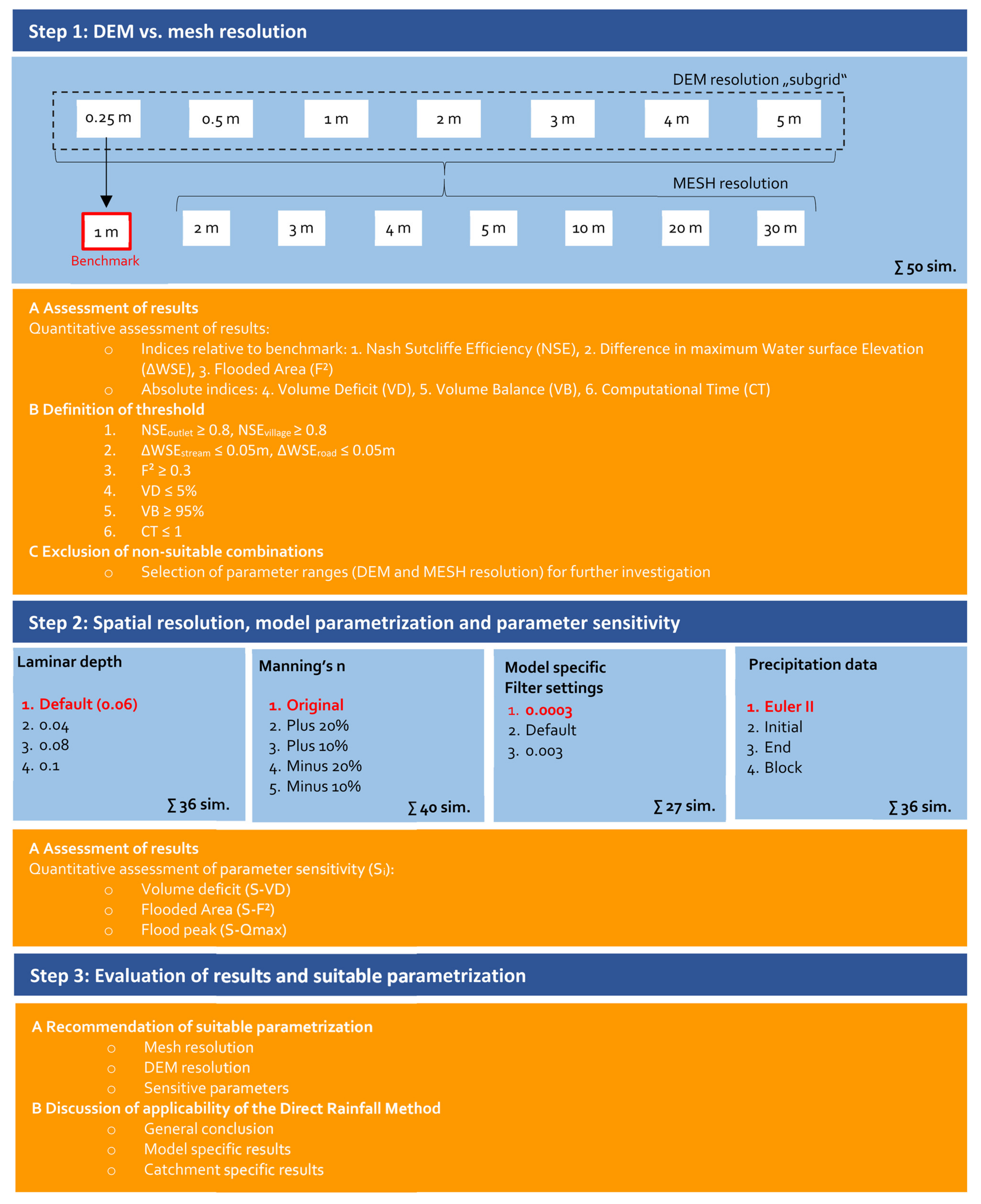
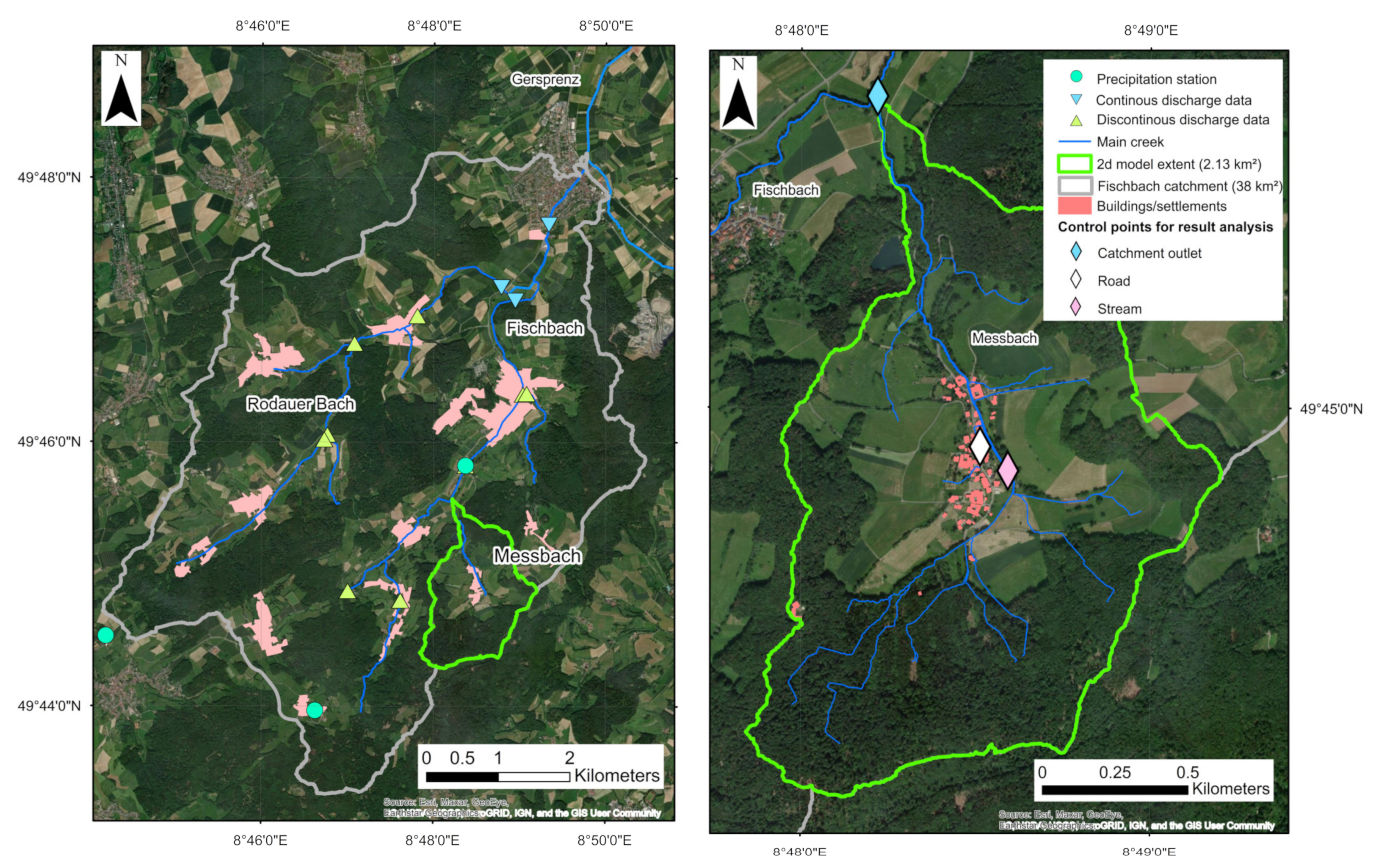
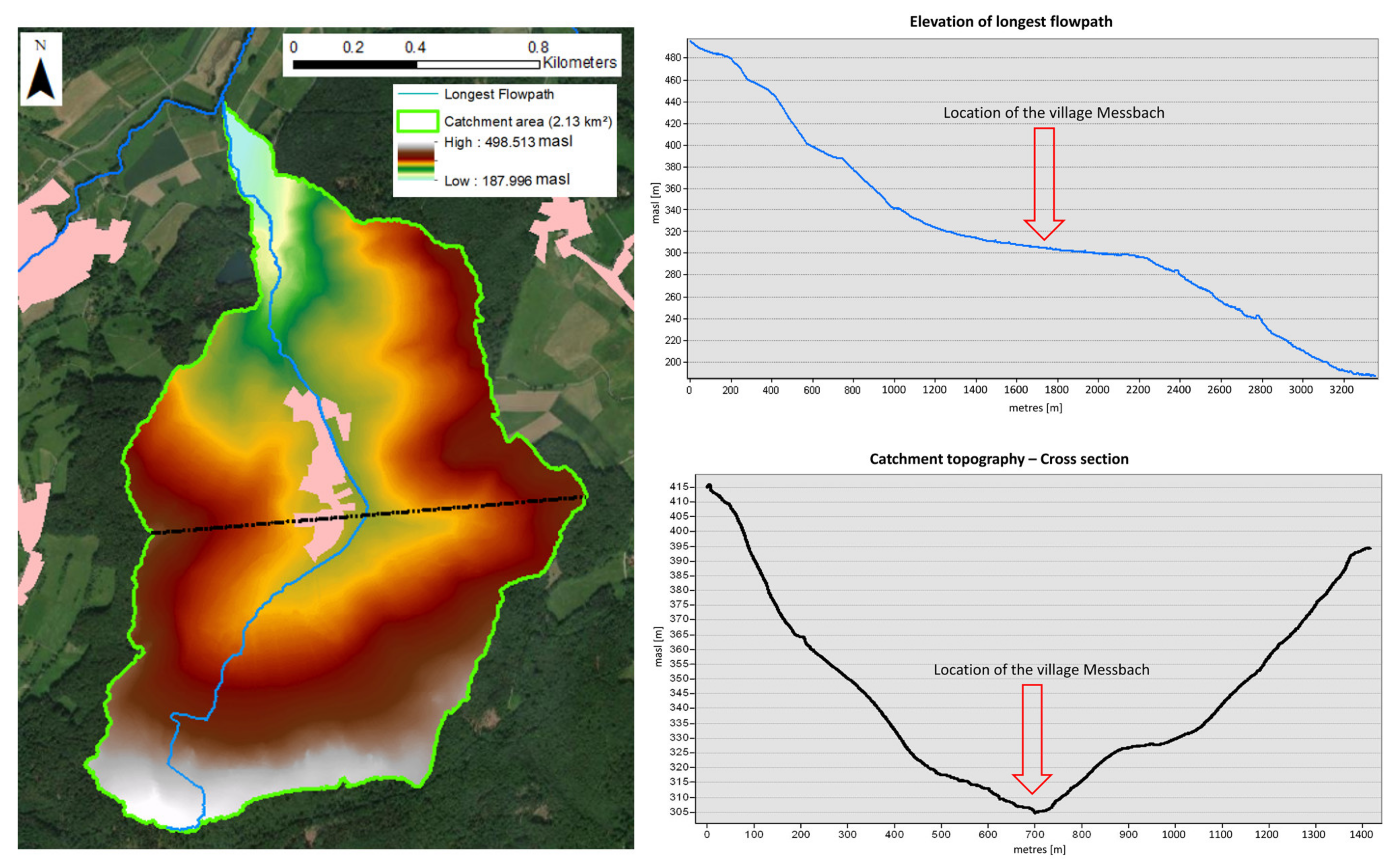
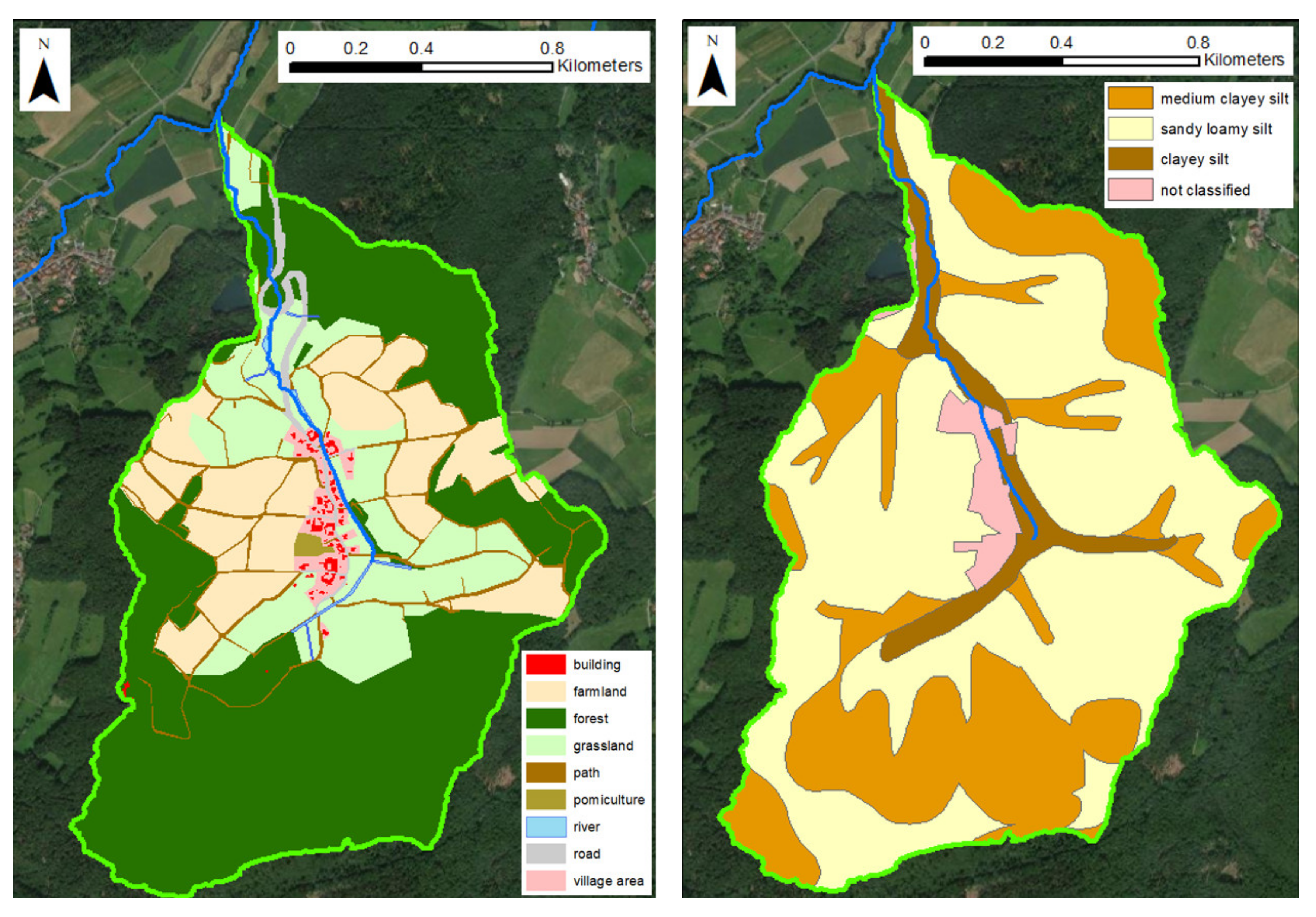
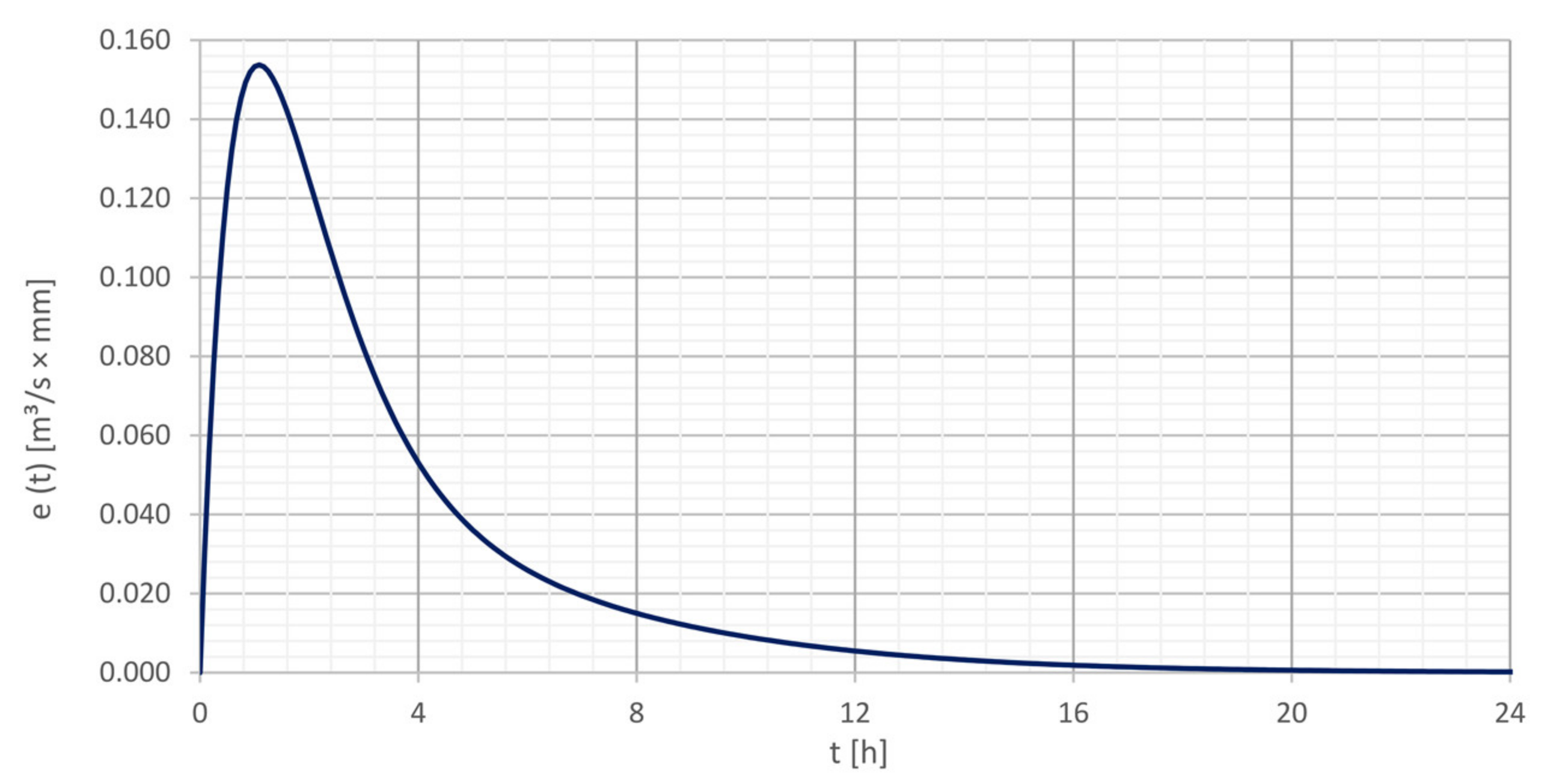
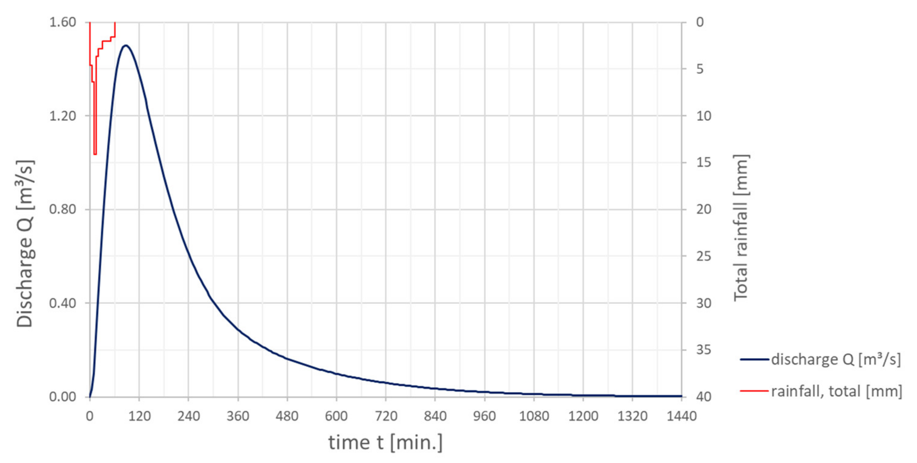
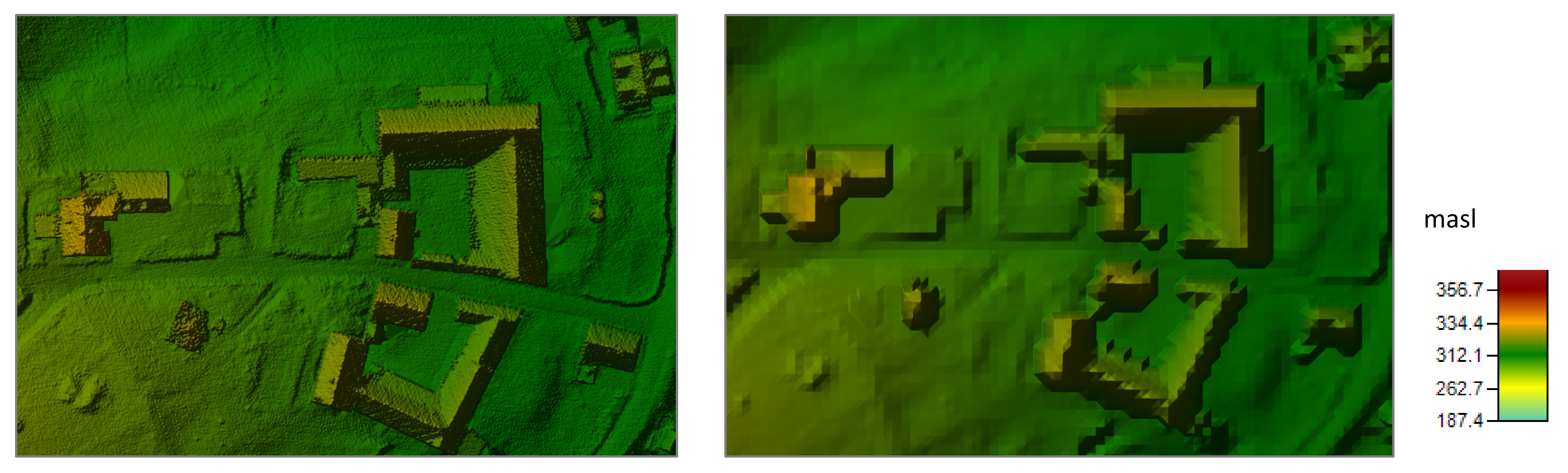
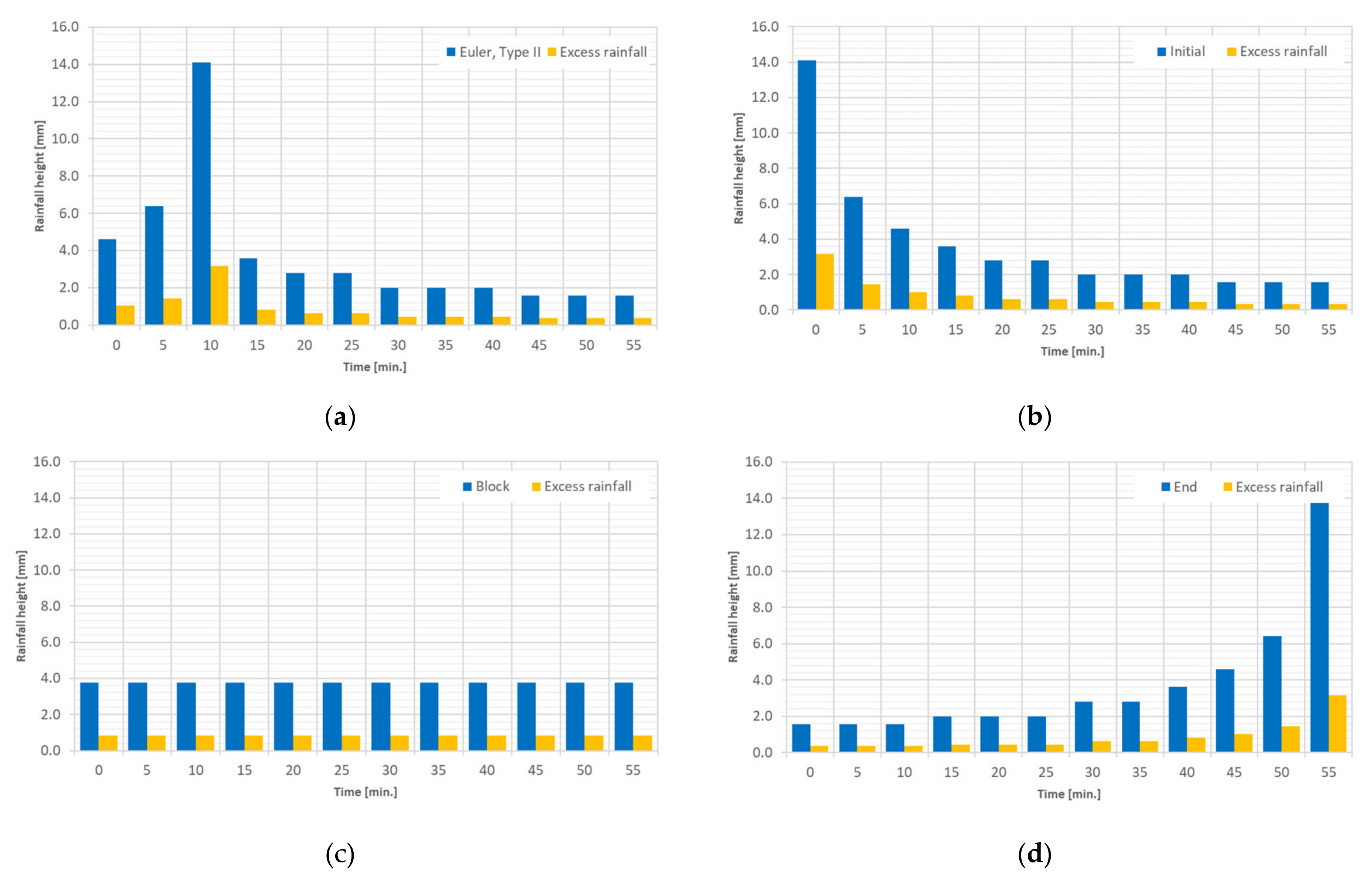
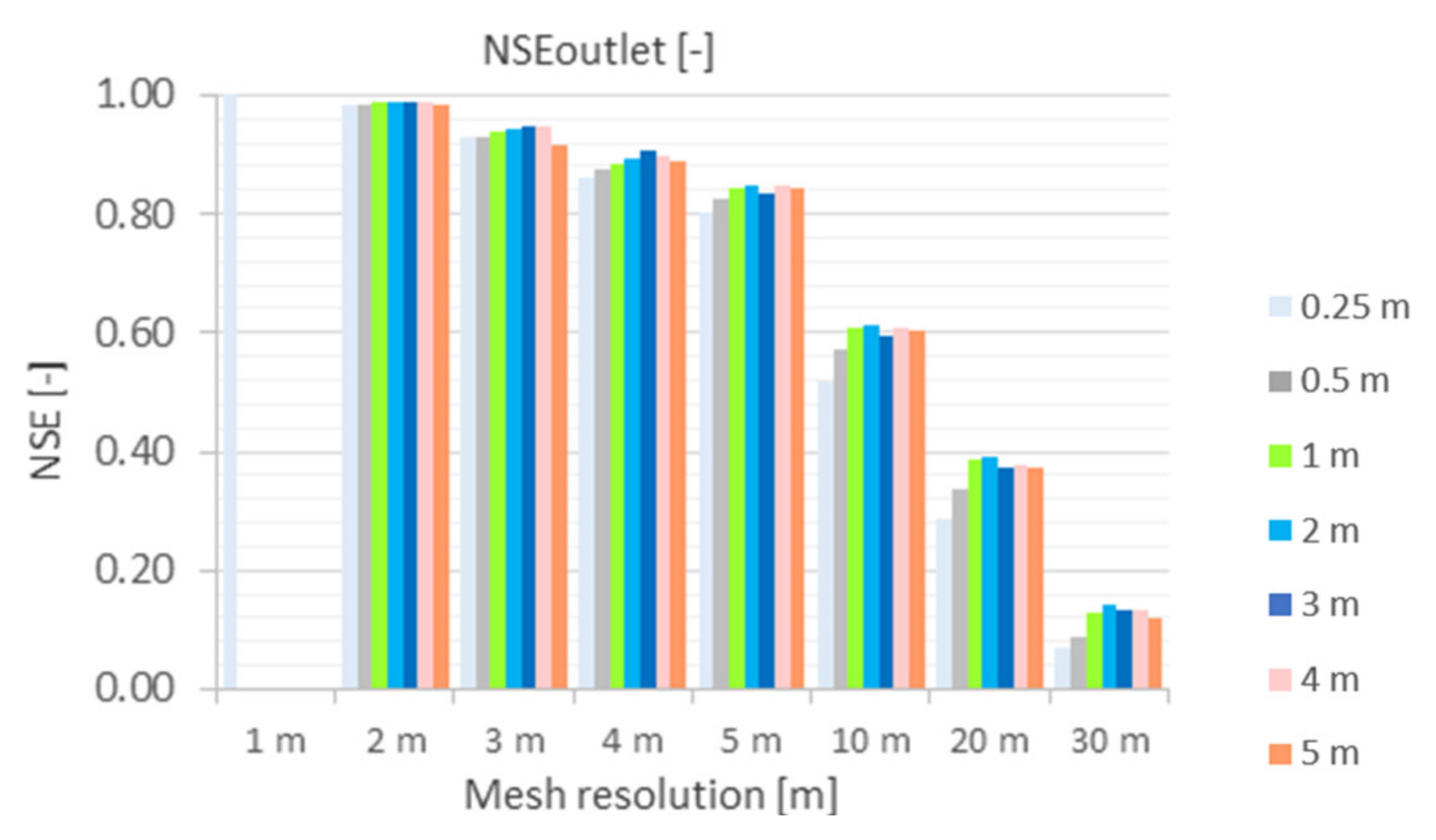
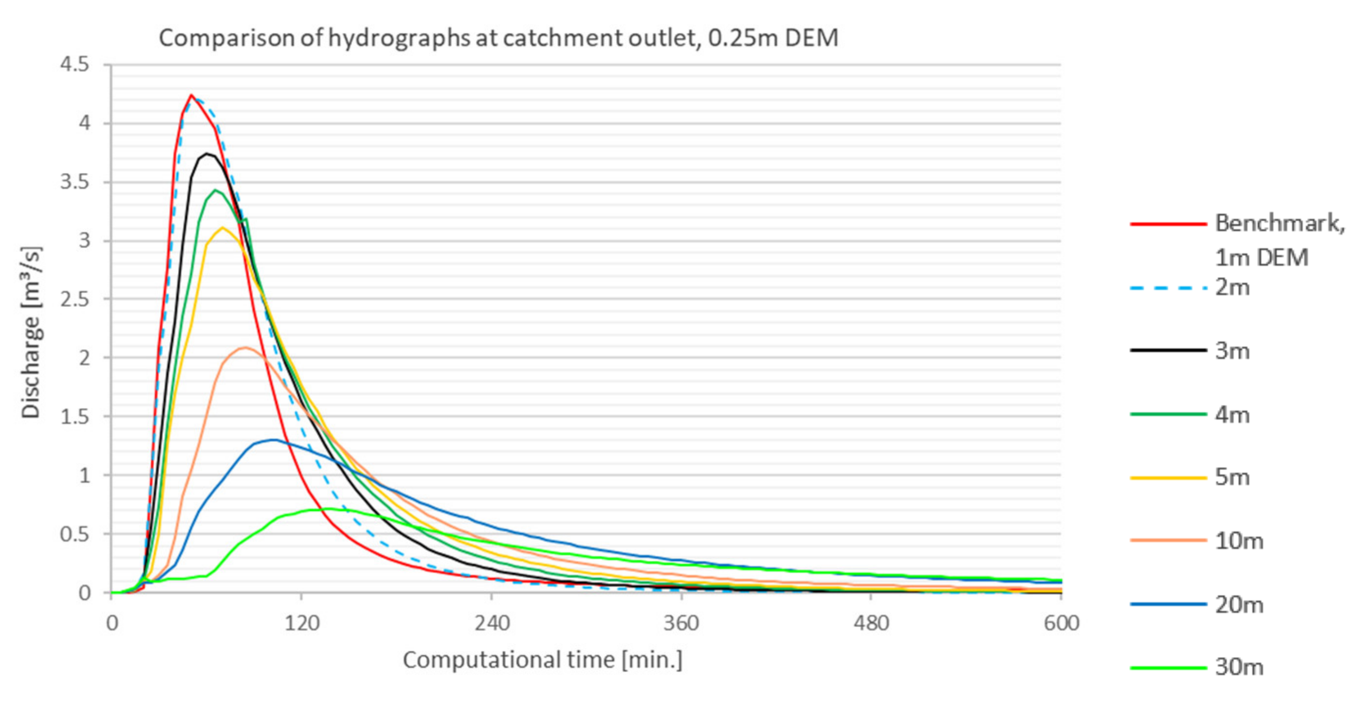
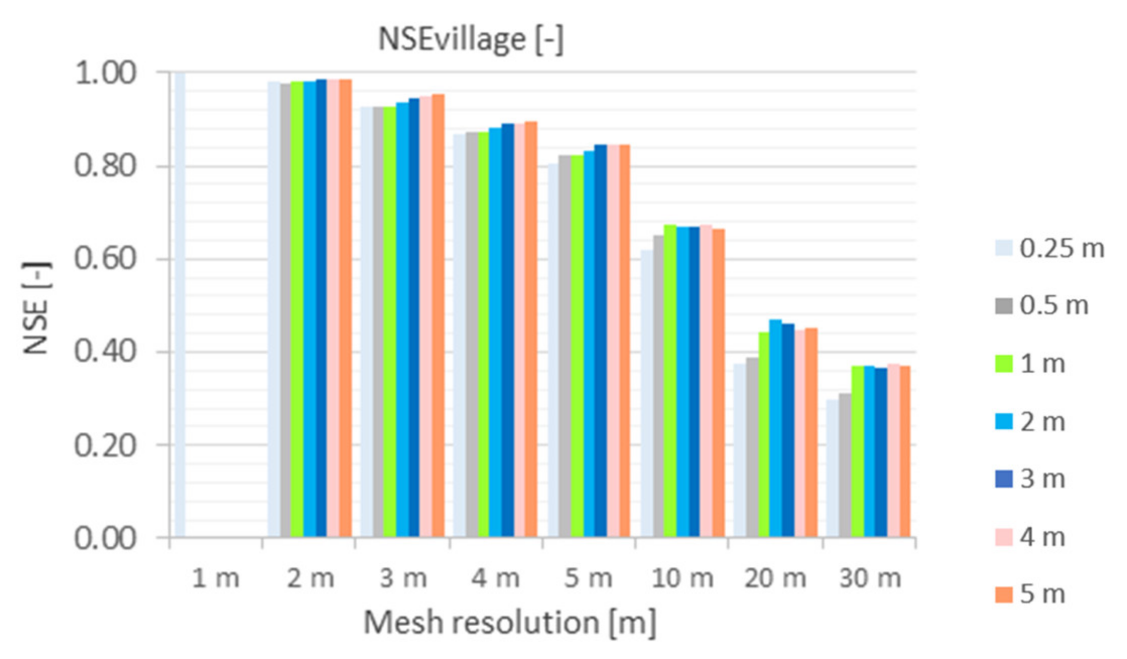
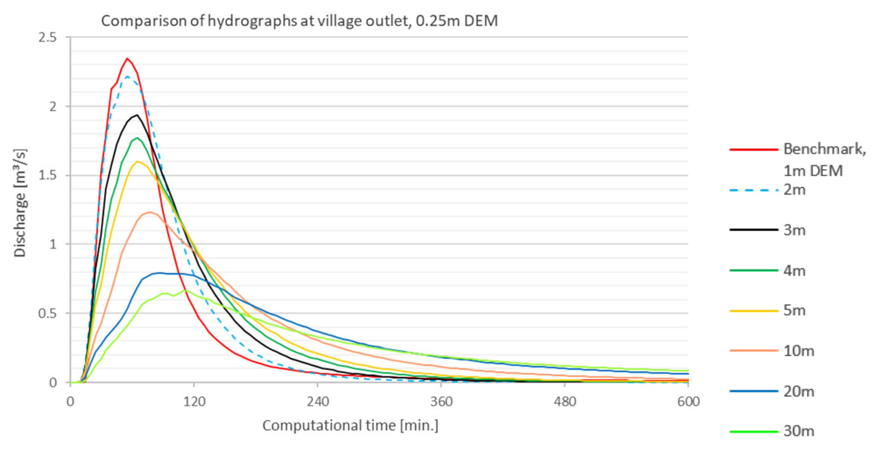
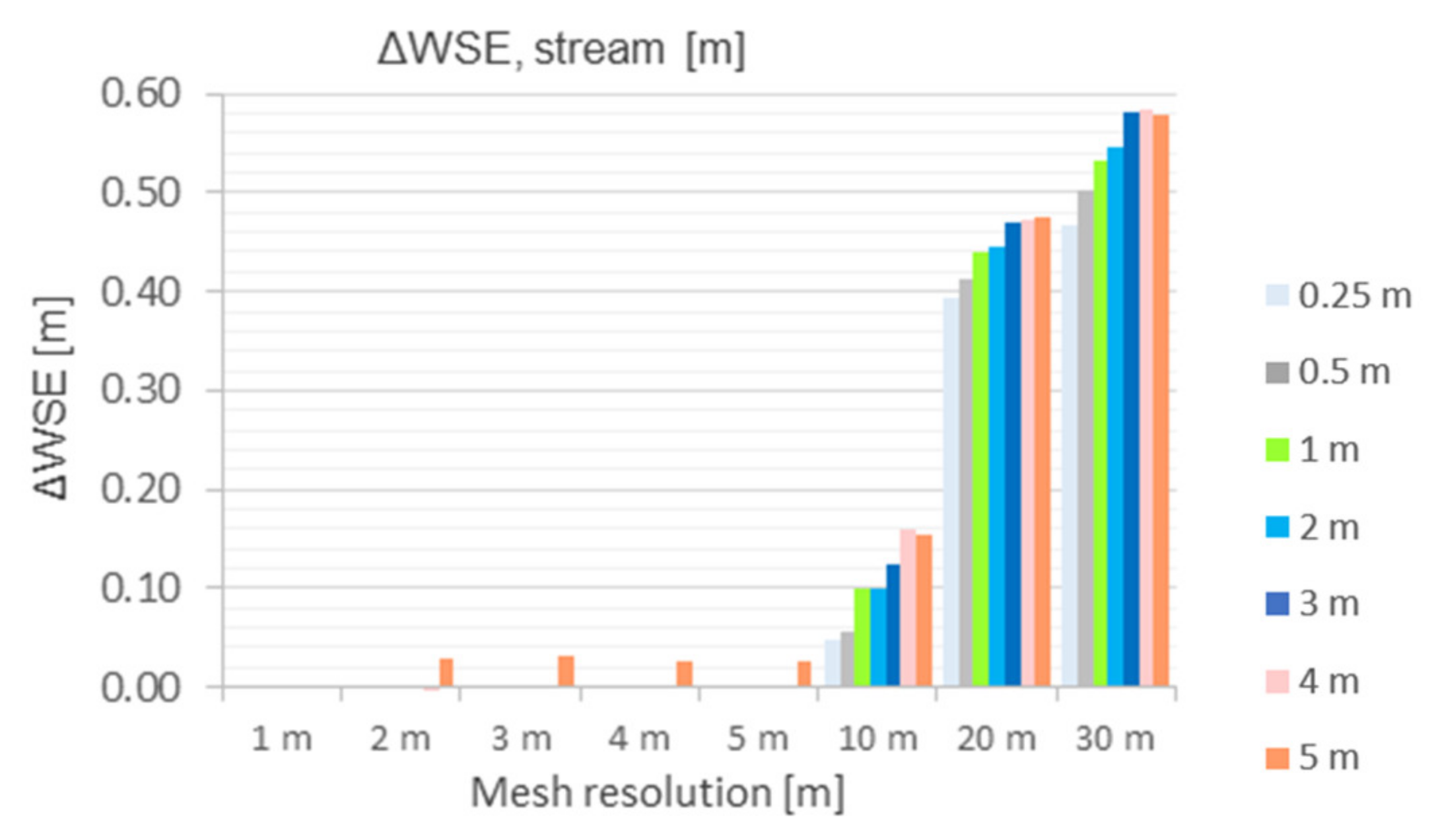
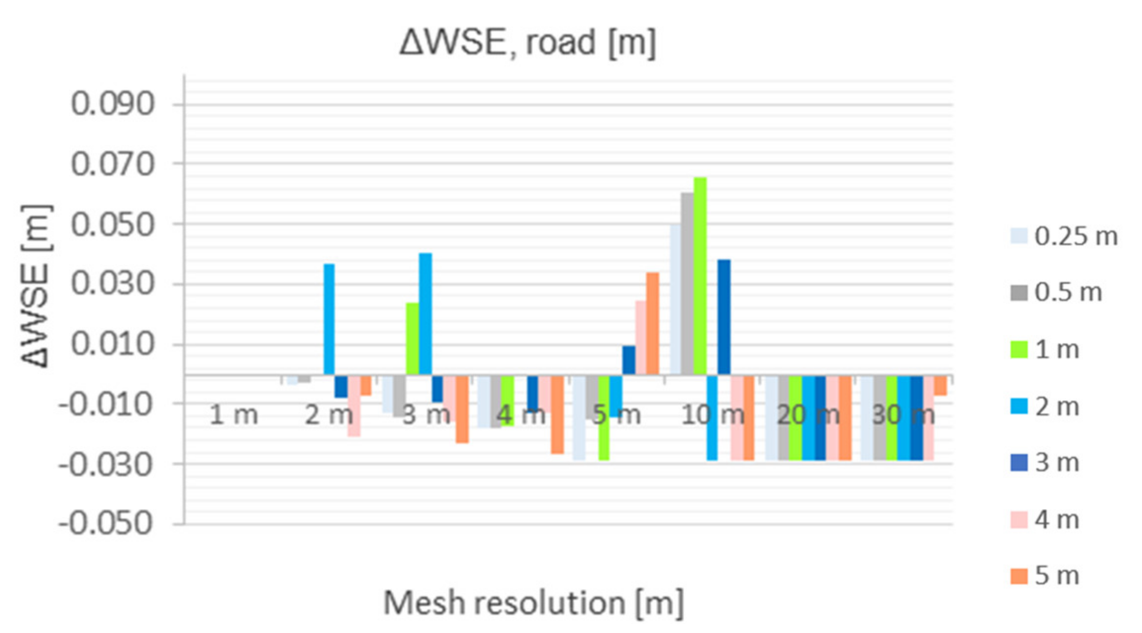
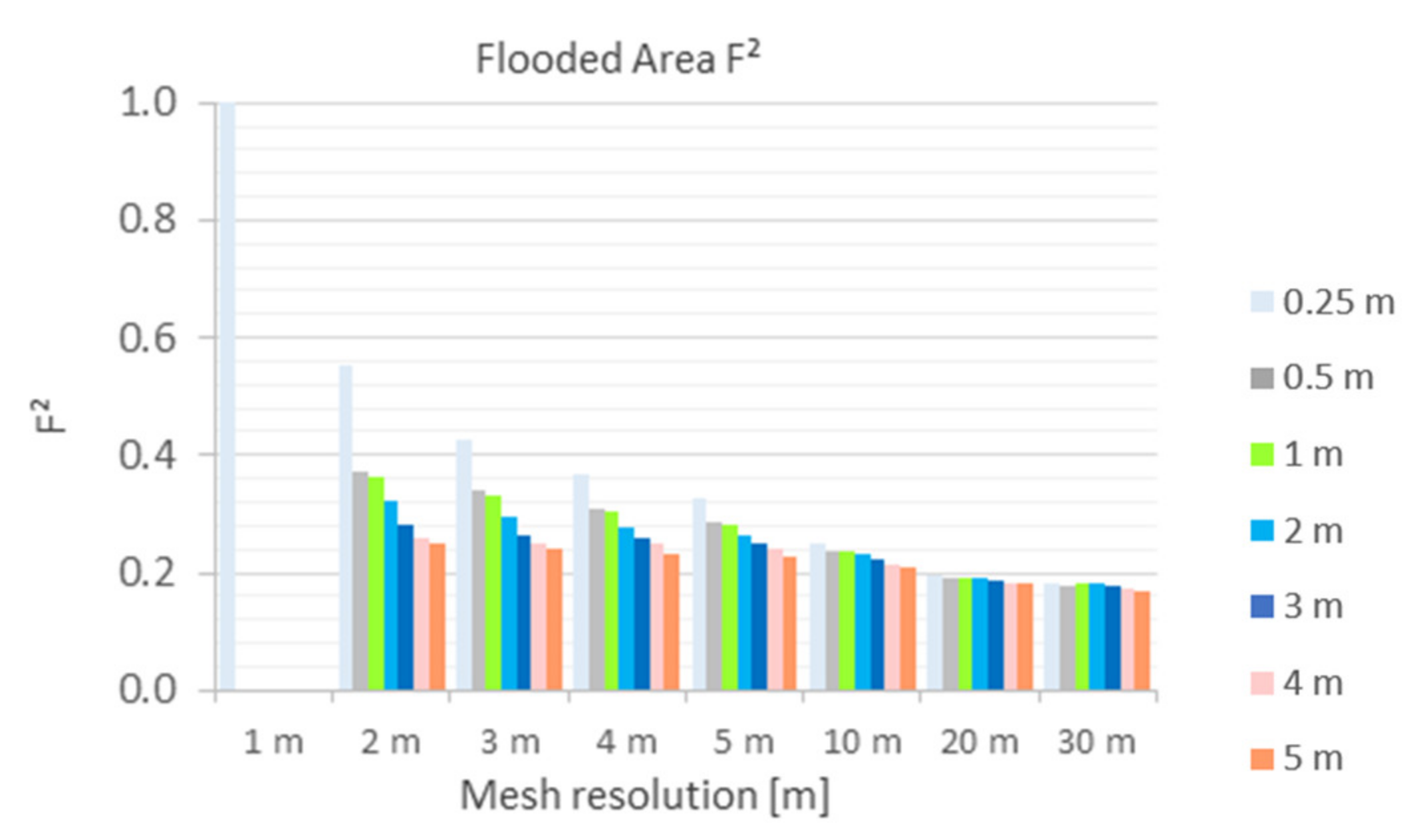
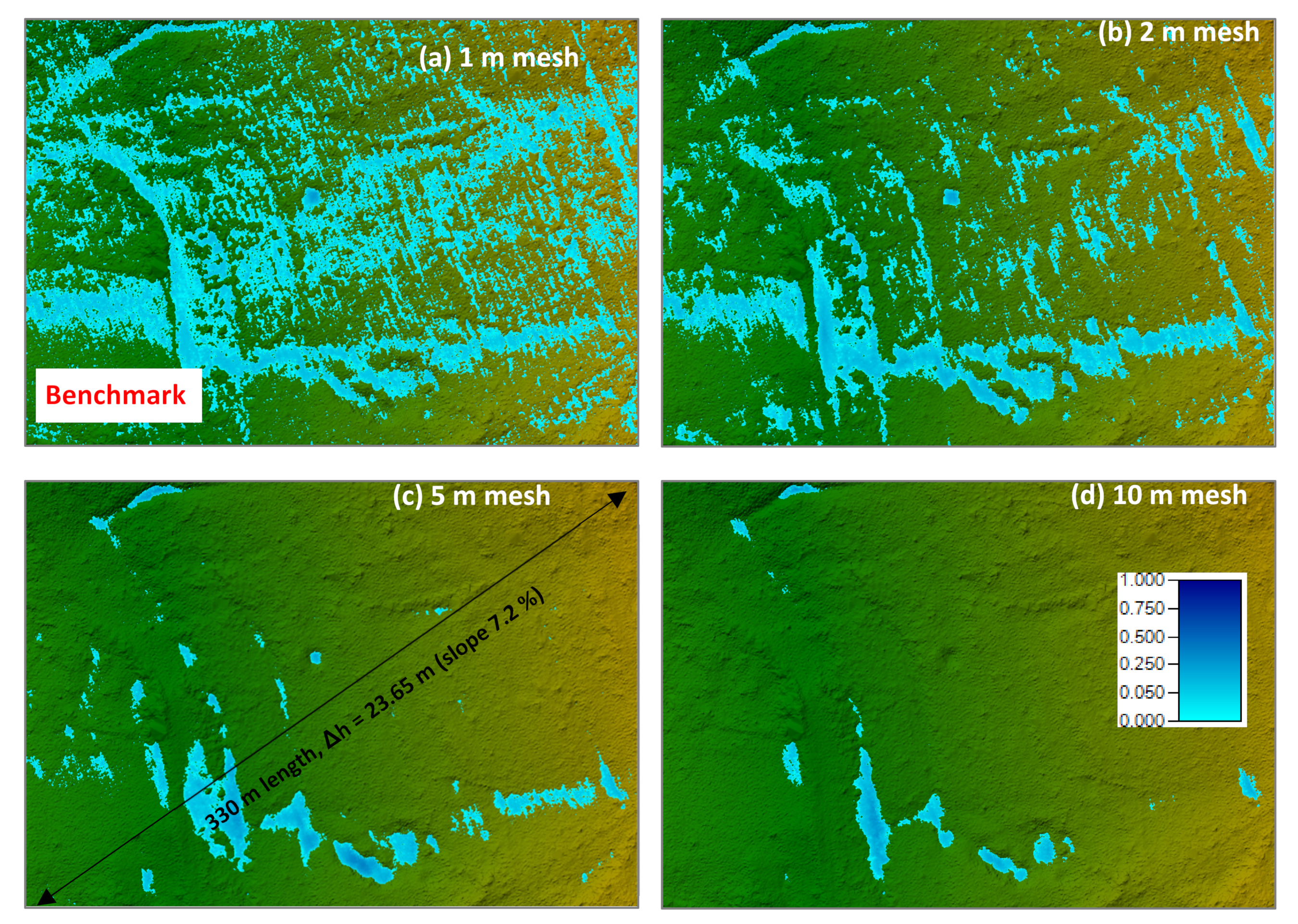
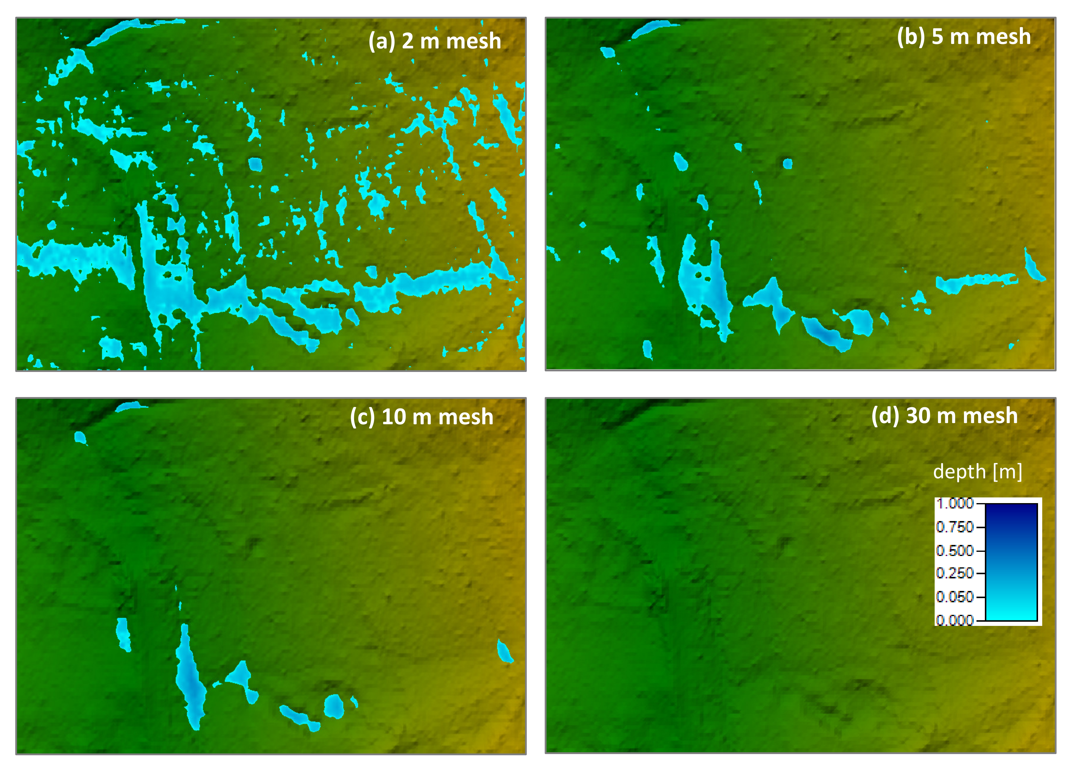
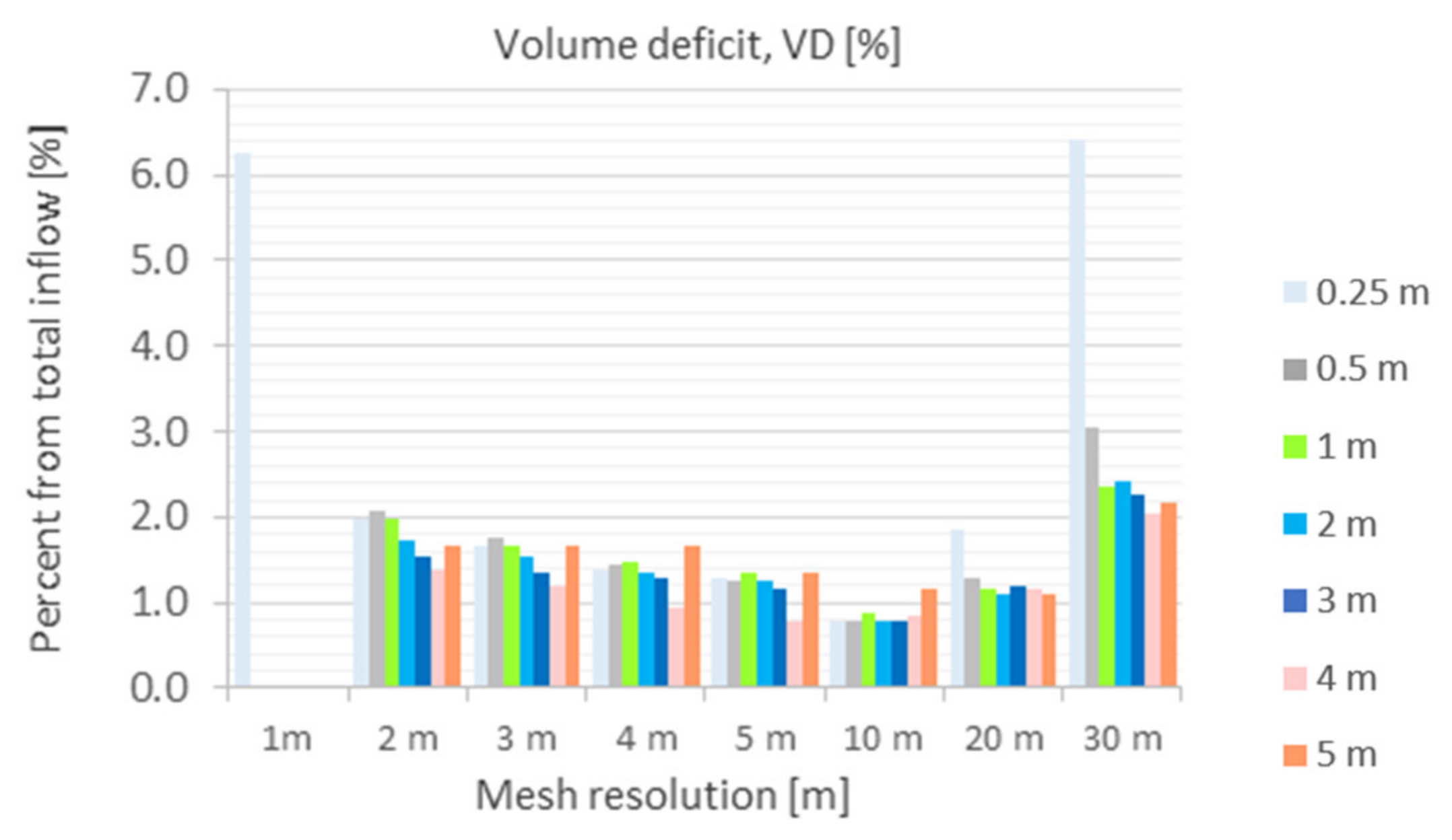
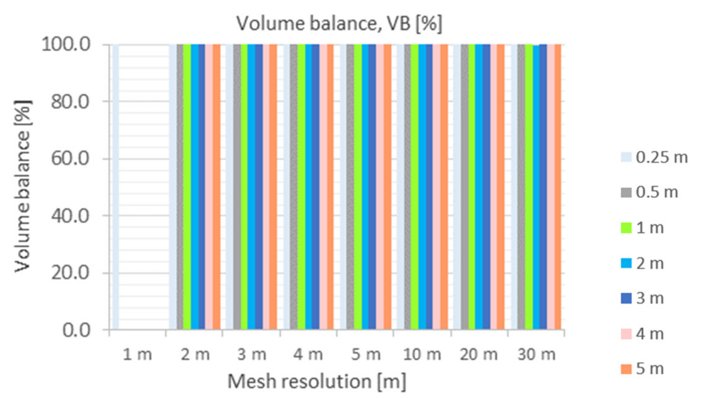
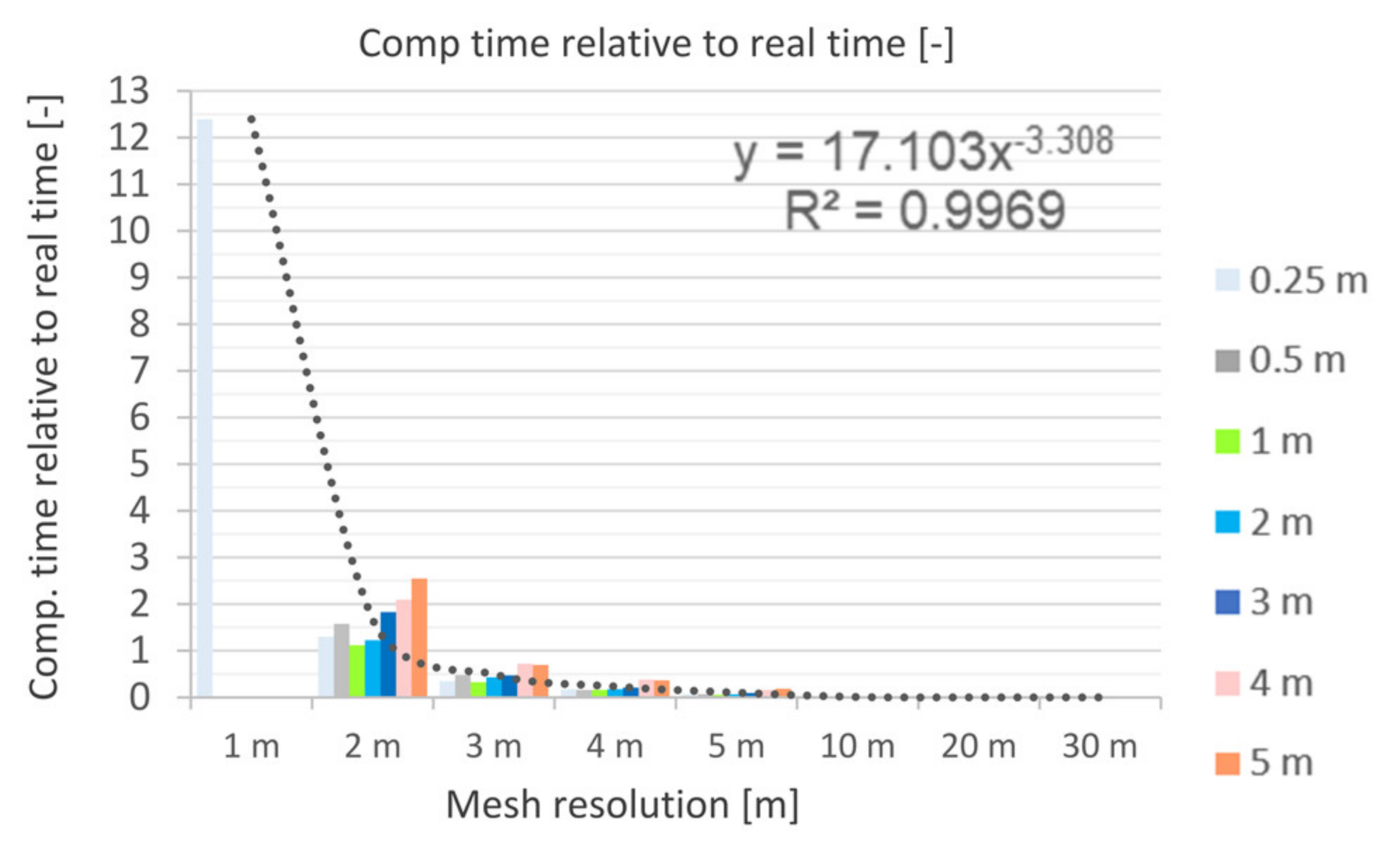
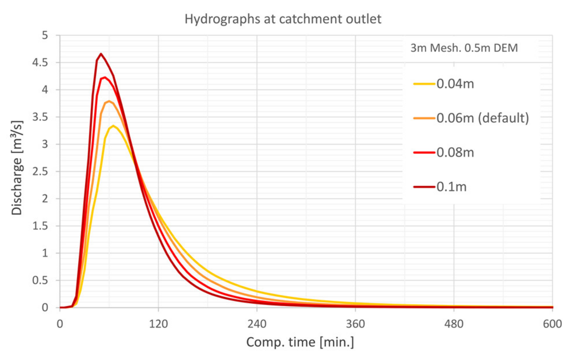
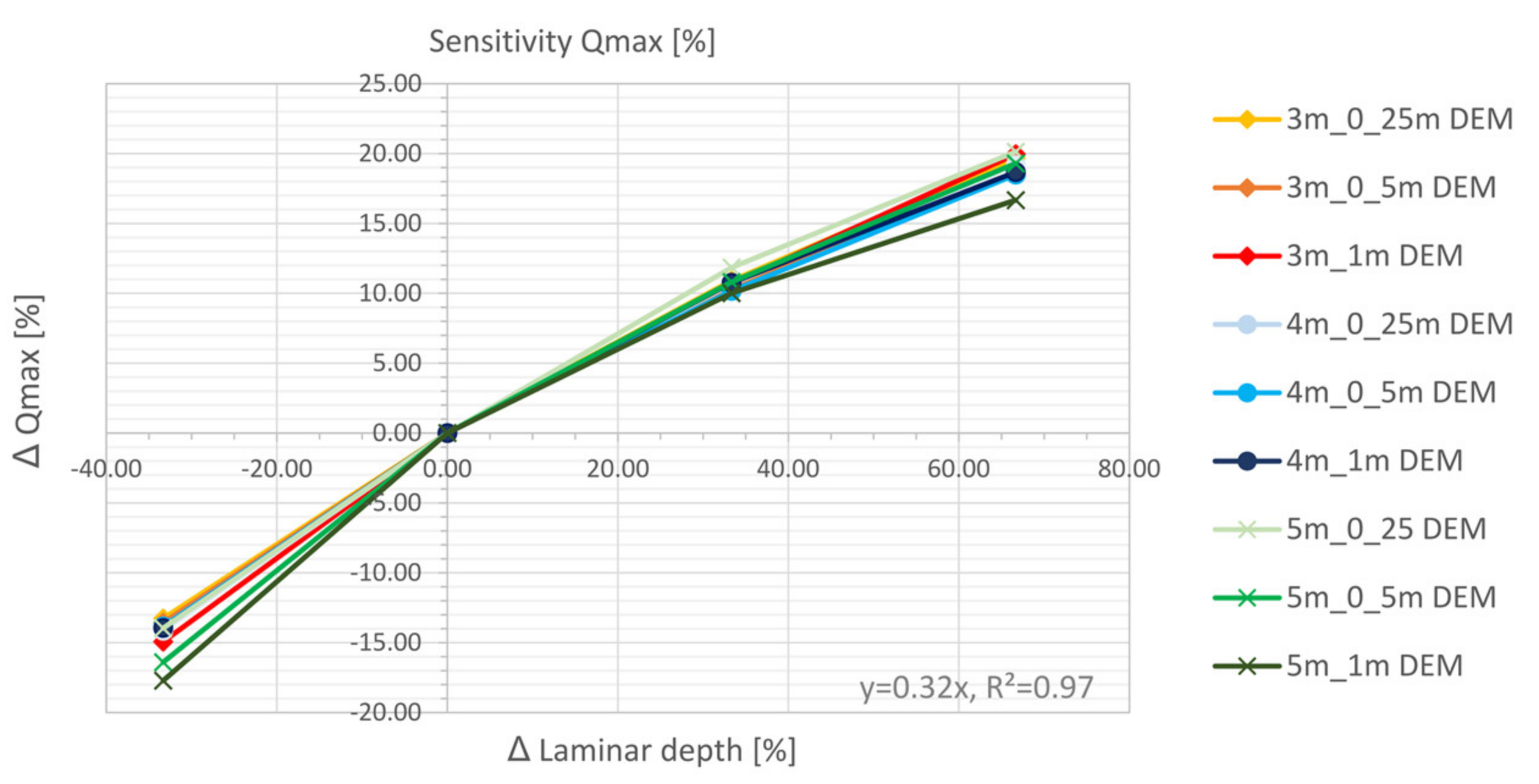
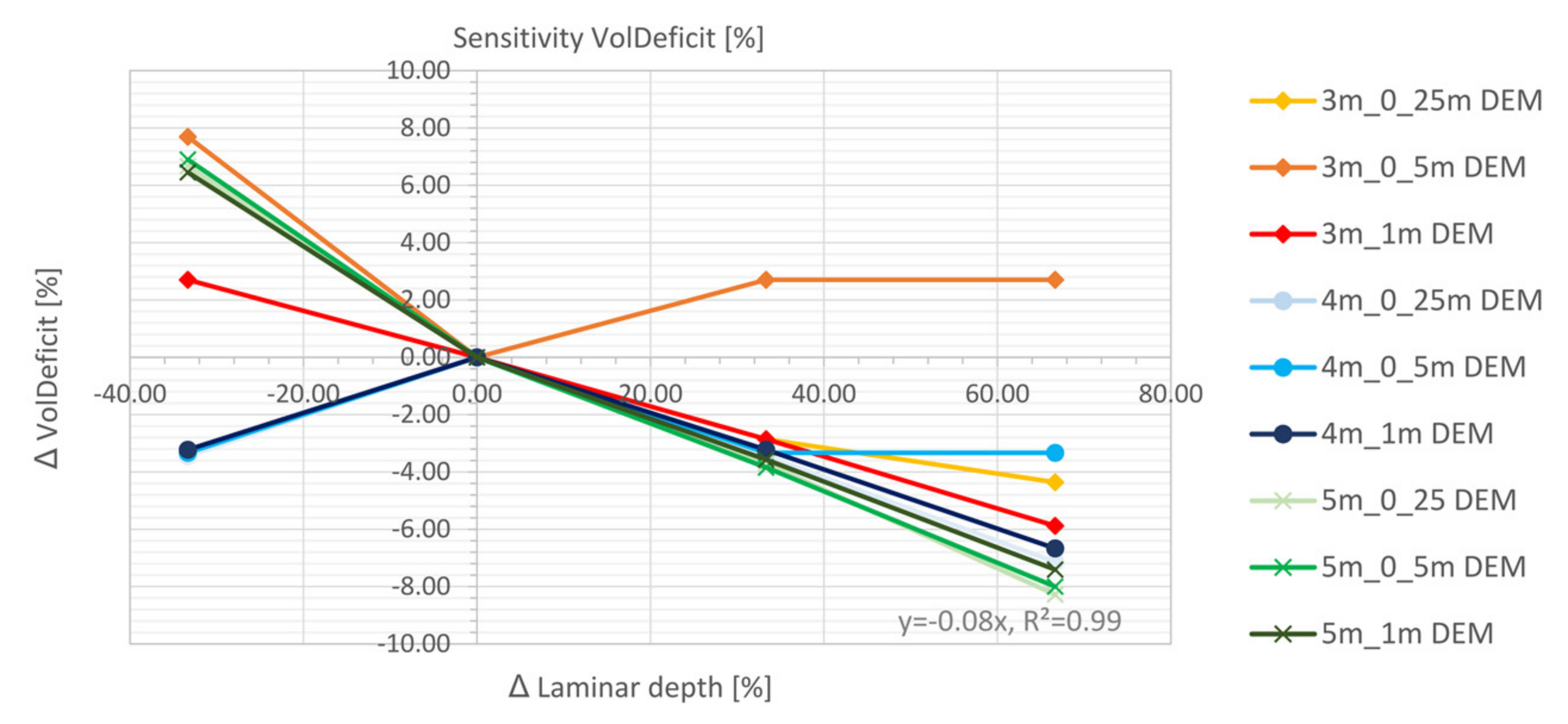
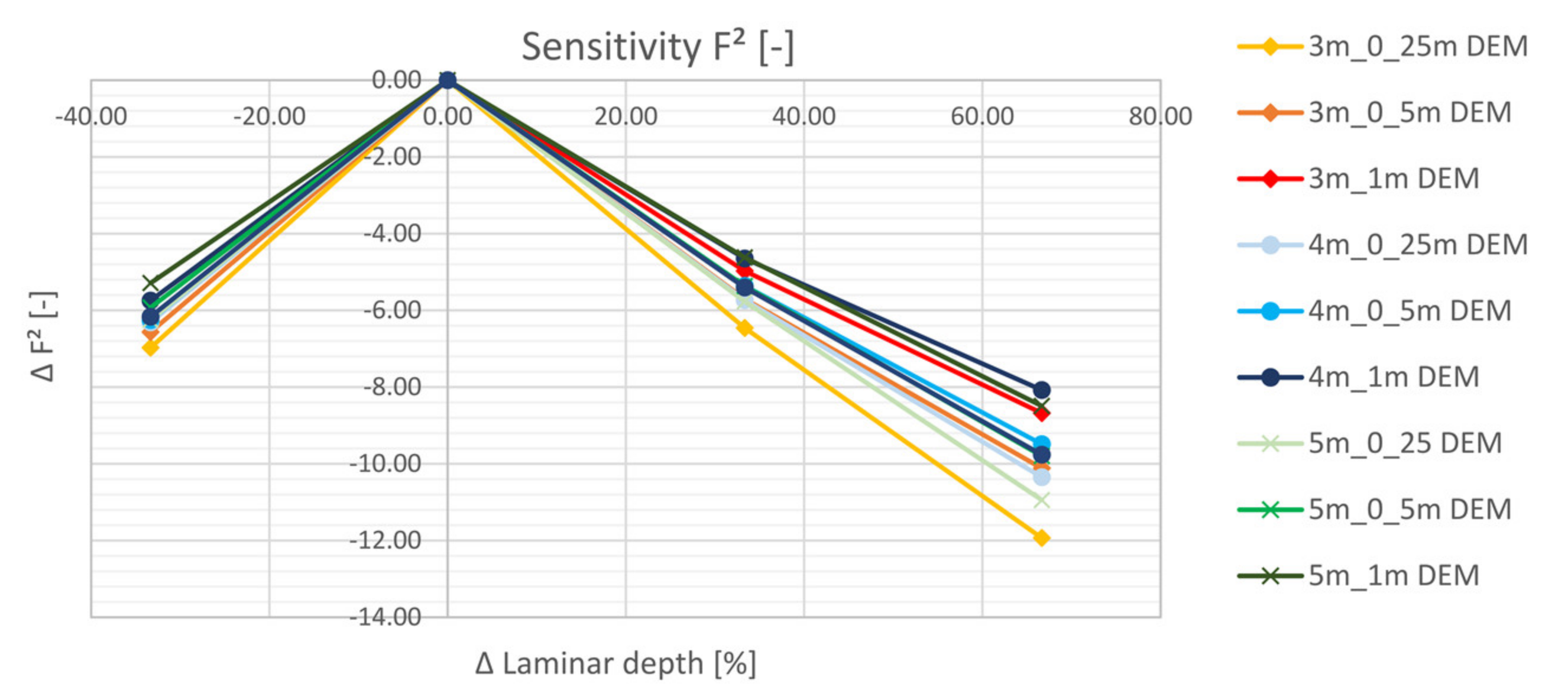
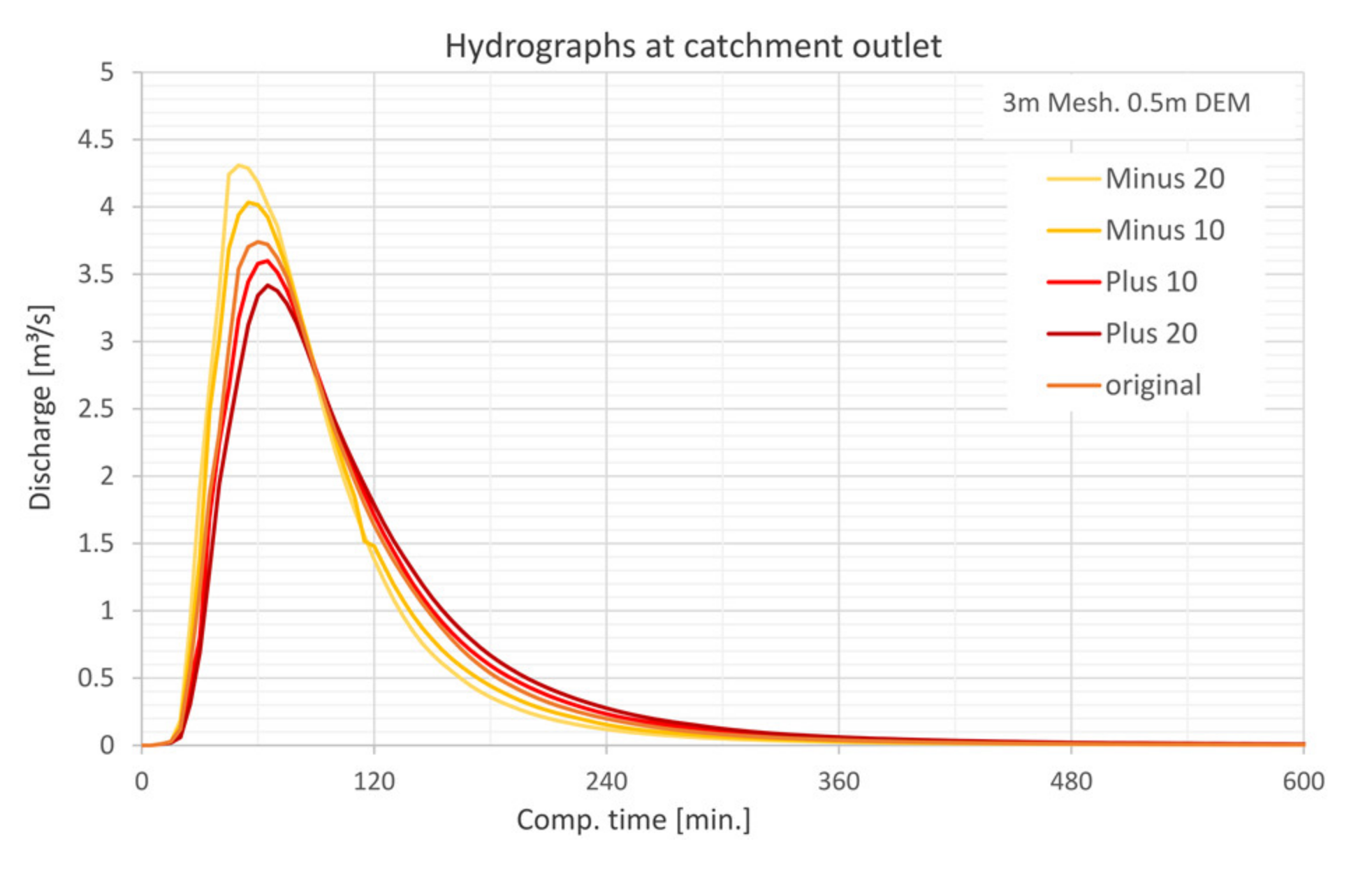
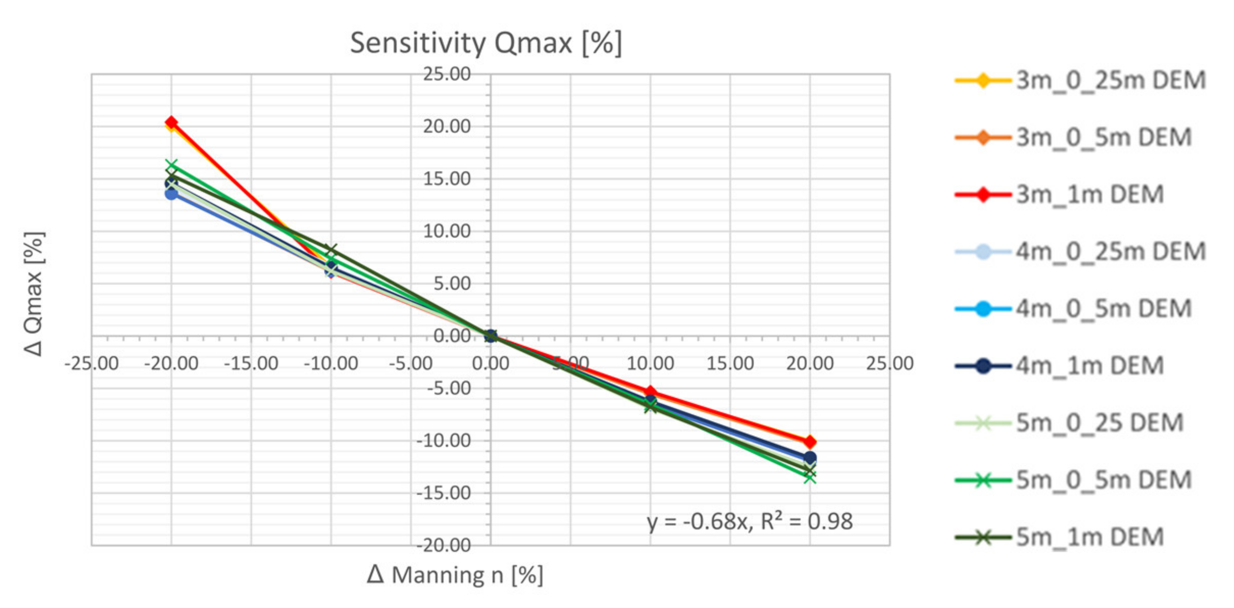
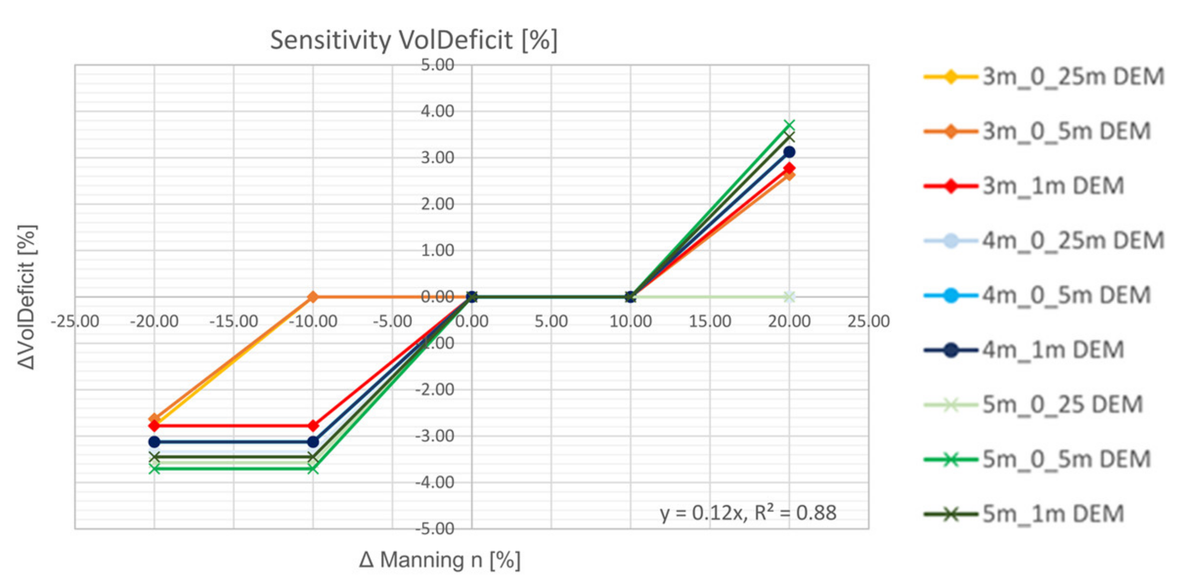
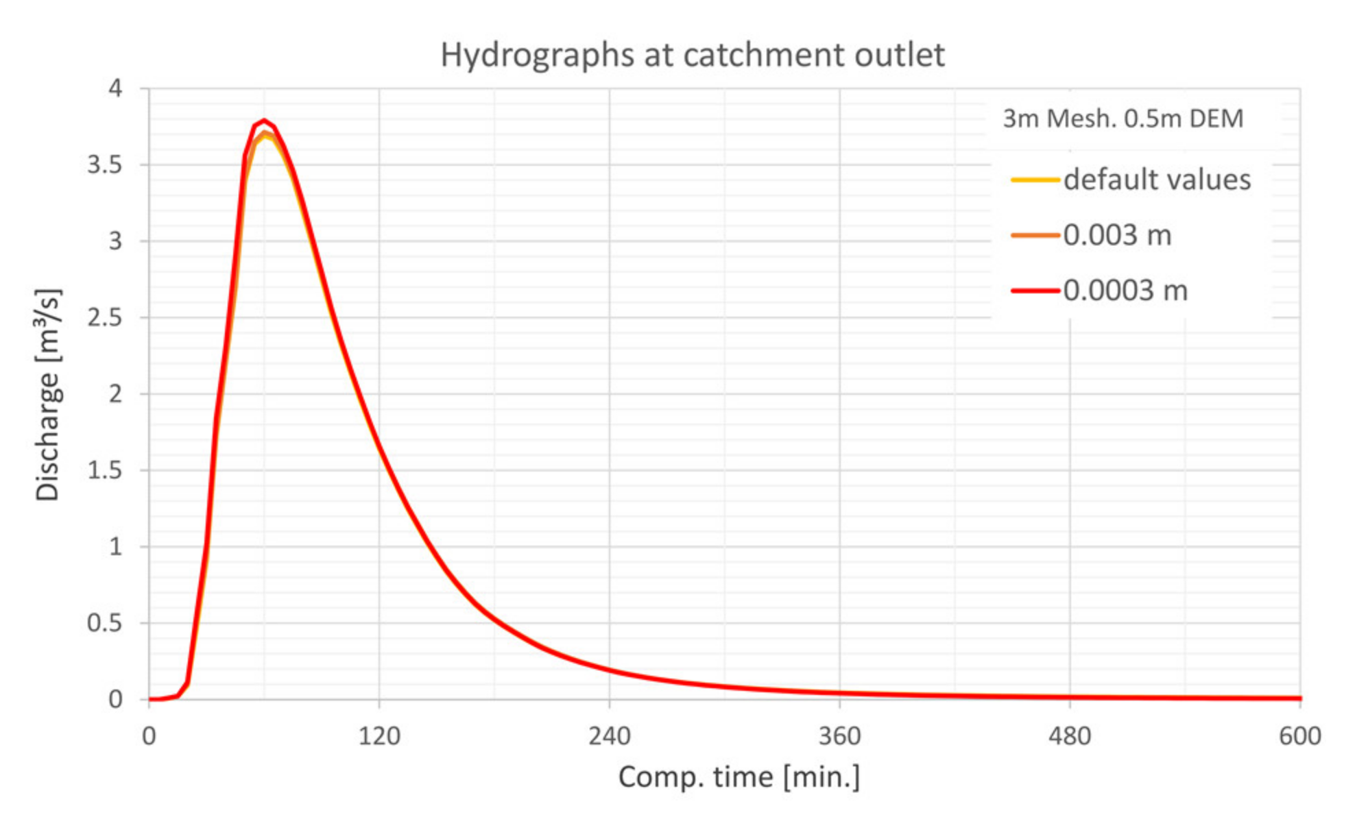
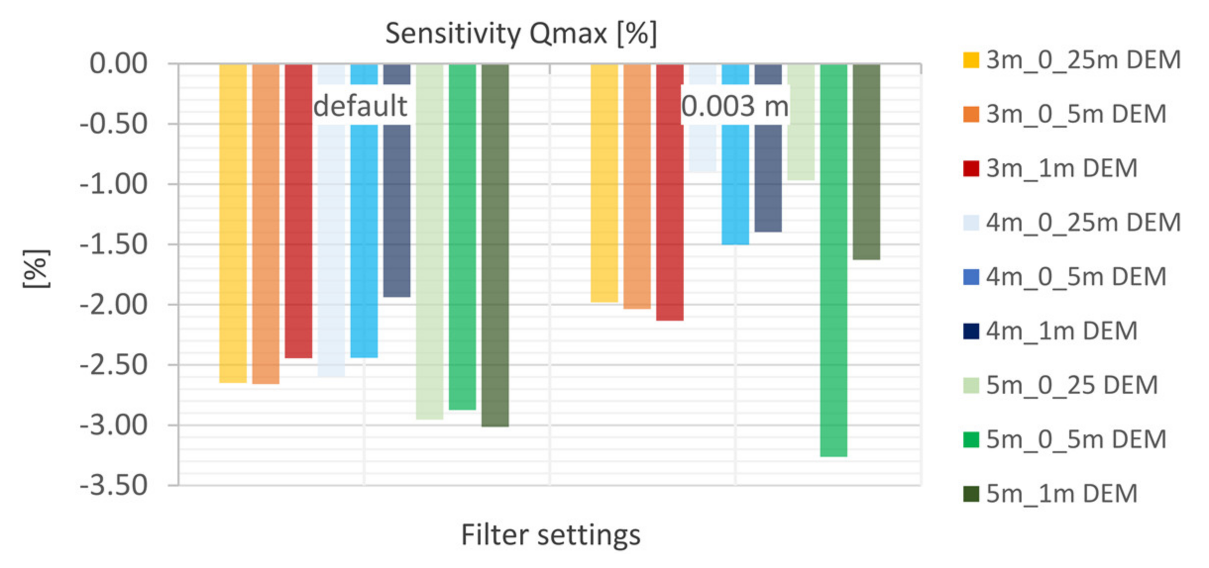
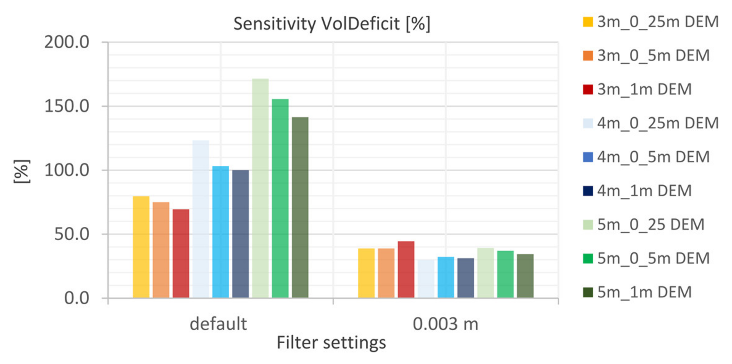
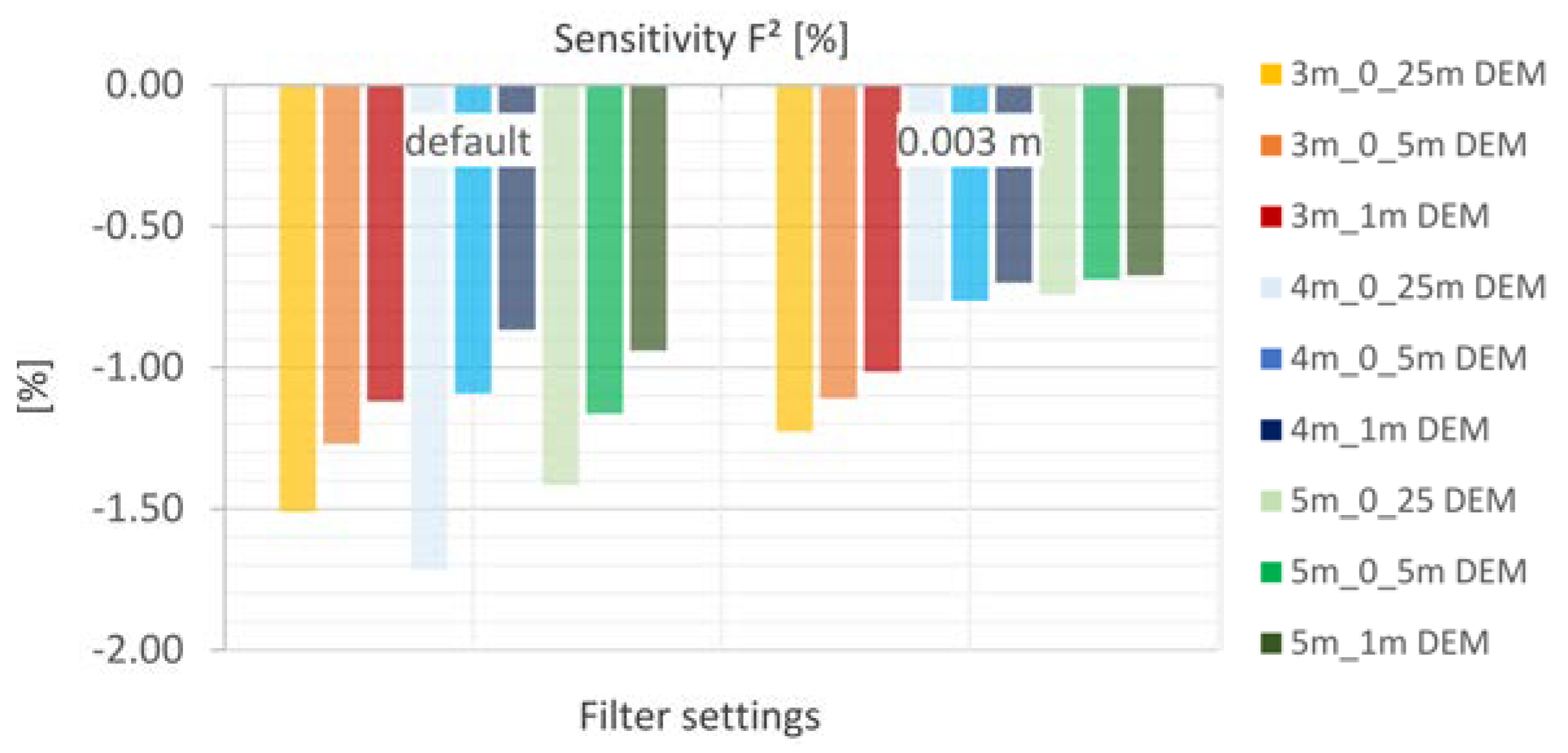
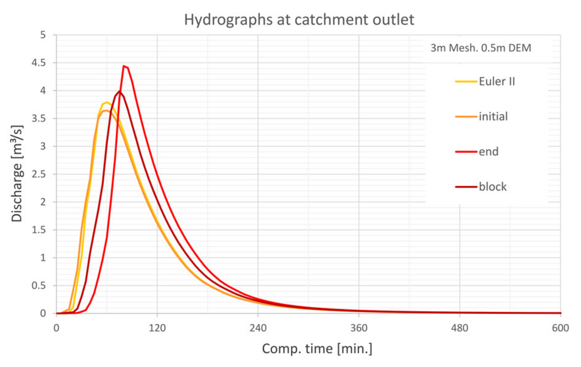
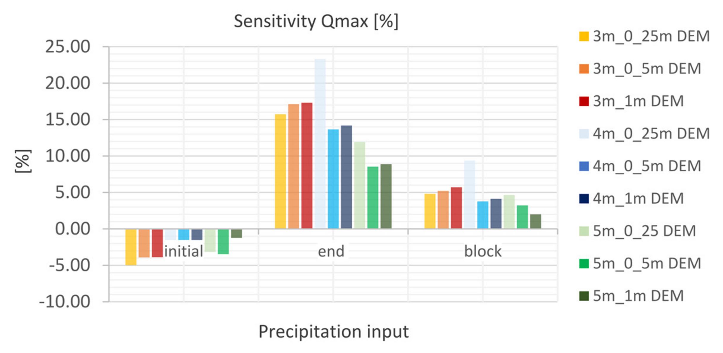
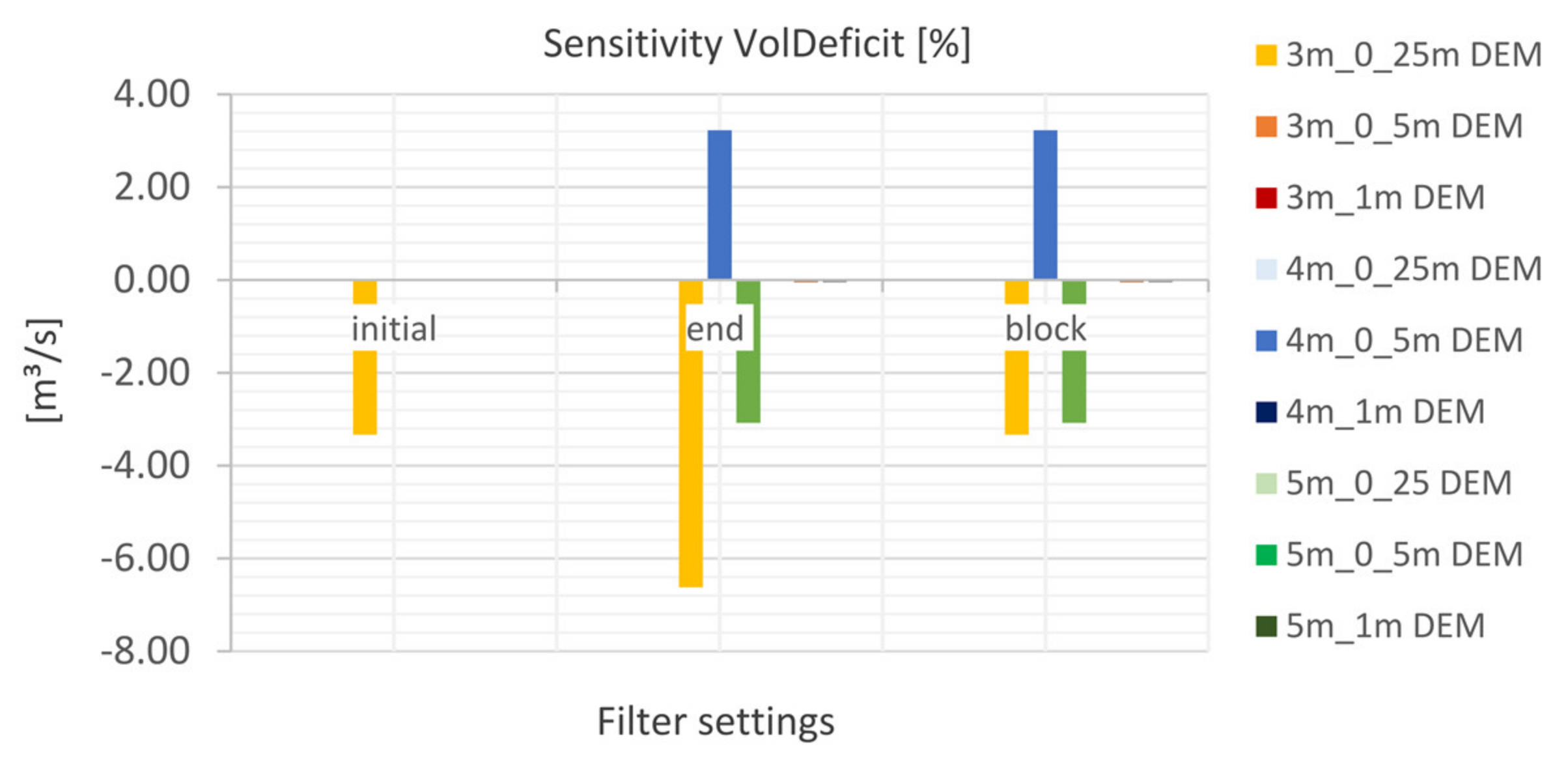
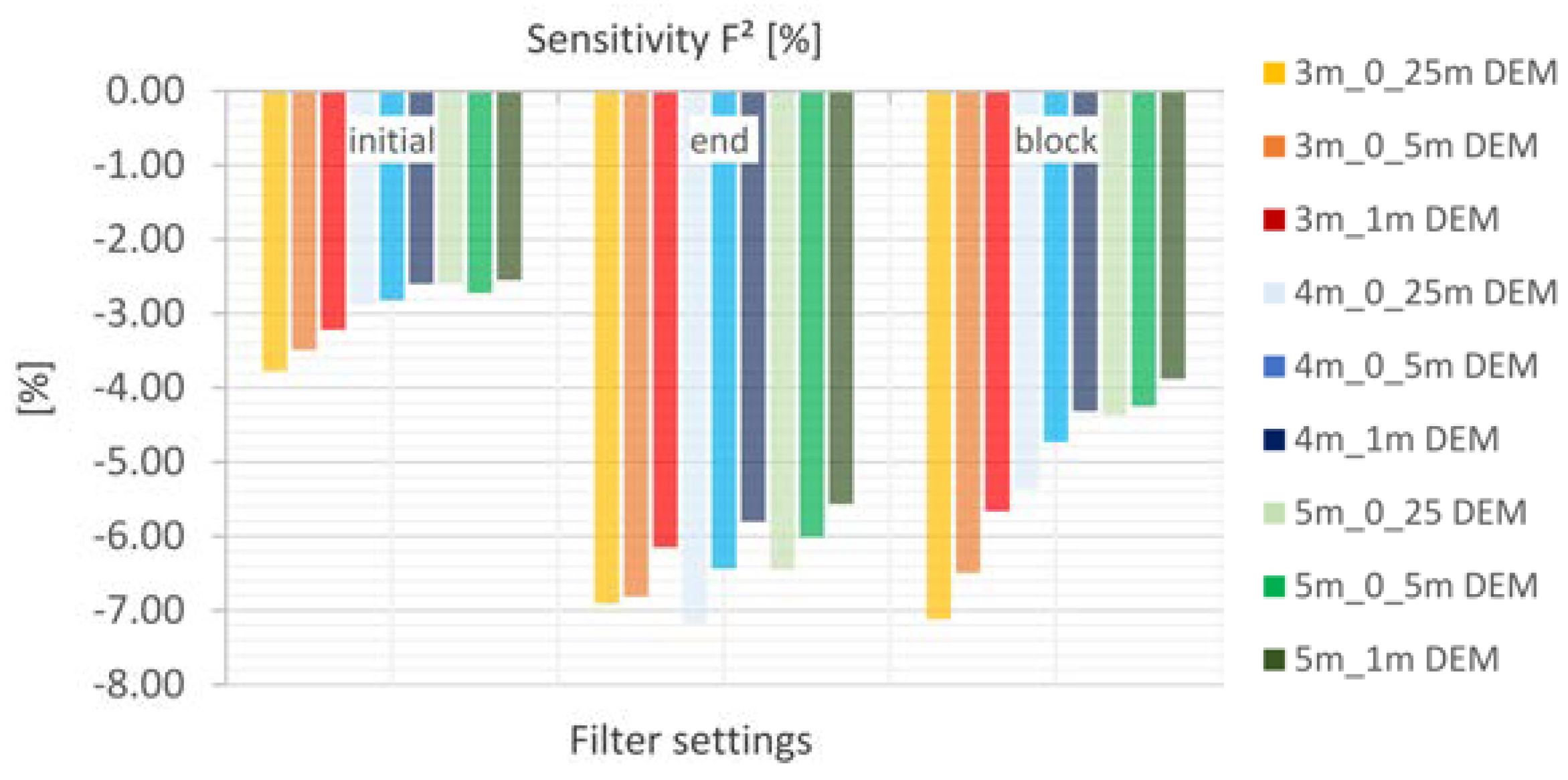
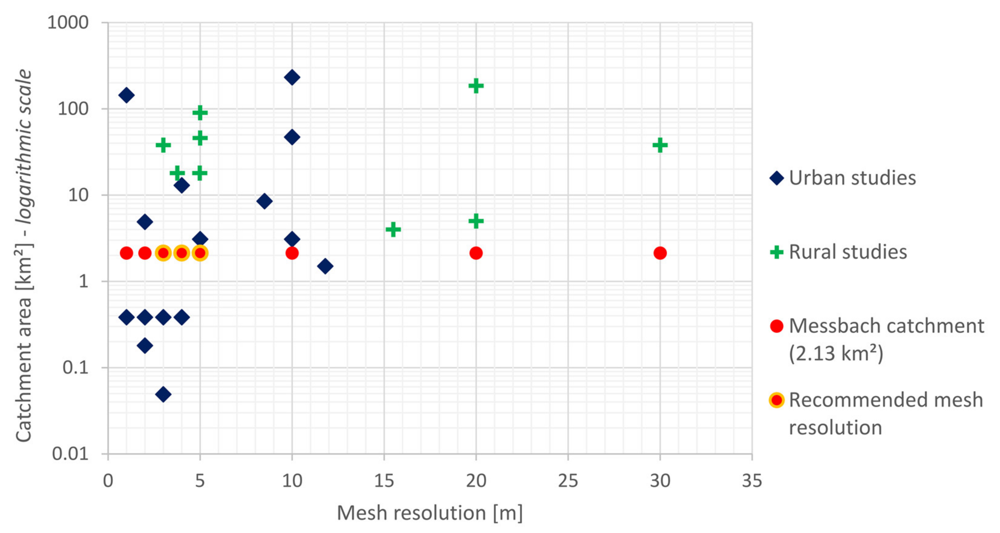
Table 1.
Overview of case studies 2D rainfall–runoff modeling (‘Direct Rainfall Method’)—Urban applications.
Table 1.
Overview of case studies 2D rainfall–runoff modeling (‘Direct Rainfall Method’)—Urban applications.
| Reference | 2D Model (s) | Catchment: Size | Spatial Resolution (Number of Cells) | Rainfall Input | Rainfall Loss Approach | Roughness Values [s×m−1/3] | Sensitivity Analysis | Calibration Data |
|---|---|---|---|---|---|---|---|---|
| Zeiger & Hubbart (2021) [3] | SWAT/ HEC-RAS | Hinkson Creek, MO: 232 km2 | DEM: 1 m Mesh: 10 m | 10 historical storm events | long term hydrological modeling (SWAT) SCS CN approach | Manning formula n from 0.003 (barren land) to 0.092 (Herbaceous); calibrated values | Computational interval | gauging stations |
| Krvavica & Rubinić (2020) [4] | HEC-RAS | Novigrad: 3.08 km2 | DEM: 2 m Mesh: 10 m, 5 m refinement (38,499 cells) | 2 historical events 6 statistical events | SCS CN approach | Manning formula n = 0.015 (roads) n = 0.2 (agriculture) | 6 different design storms 4 different rainfall durations | none |
| Caviedes-Voullième et al. (2020) [17] | in-house development | Glasgow: 0.384 km2 | 4 m (24,100) 3 m (42,693) 2 m (96,400) 1 m (384,237) | 1 rainfall event | none | Manning formula n = 0.02 (roads) n = 0.05 (other) | SWE and ZI (‘zero inertia’) solver mesh resolution | none |
| Rangari et al. (2019) [16] | HEC-RAS | Hyderabad: 47.08 km2 | DEM: 10 m Mesh: 10 m (139,487) | 3 historical events 3 statistical events | no information | Manning formula n = 0.025 | none | none |
| Tyrna et al. (2018) [8] | FloodArea | Unna: 144 km2 | 1 m (144,000,000) | 1 statistical event 1 fictional event | simplified physical approach based on Green and Ampt and Darcy | Manning formula from n = 0.013 (roads) to n = 0.250 (forest) | none | none |
| Pina et al. (2016) [18] | Infoworks ICM v.5.5 | Cranbrook: 8.5 km2 Zona central: ca. 1.5 km2 | Cranbrook: avrg. 8.5 m (117,712) Zona central: avrg. 11.8 m (10,741) | Cranbrook: 3 historical events, 5 statistical events Zona central: 4 historical events, 6 statistical events | fixed runoff coefficient | no information | SD/FD approach different design storms | gauging station |
| Cea & Rodriguez (2016) [19] | GUAD-2D | Alginet: 12.97 km2 | 4 m (ca. 810,625) | 500-year event | SCS CN approach Green-Ampt Horton Philip | Manning formula | hydraulic-hydrological calculation | none |
| Fraga et al. (2016) [20] | in-house development | Motorway section: 0.049 km2 | avrg. 3 m (ca. 5444) | 7 historical events | initial- constant approach | Manning formula n = 0.02–0.1 (impervious surface) n = 0.02–0.5 (pervious surface) n = 0.008–0.025 (conduits) | Manning’s n Infiltration rates Discharge coefficients | discharge data |
| Leandro et al. (2016) [23] | P-DWave | Borbecker Mühlenbach: 4.9 km2 | 2 m (ca. 1,225,000) | 1 historical event | Green-Ampt | Manning formula | 5 modeling levels, increasing complexity of key urban features | none |
| Yu et al. (2015), [2] | FloodMap | City of Kingston/Hull: - | 10 m 20 m | 1 historical event | Green-Ampt | Manning formula | Mesh resolution Manning’s n Hydraulic conductivity | inundation areas |
| Néelz & Pender (2013) [25] Karl Broich et al. (2018) [26] Brunner (2018) [27] | Various | Glasgow: 0.384 km2 | 2 m (ca. 97,000) HEC-RAS: DEM: 0.5 m Mesh: 2 m, 4 m | 1 event | none | Manning formula 0.02 (roads) 0.05 (area) | HEC-RAS: mesh resolution | none |
| Chen et al. (2010) [28] | Sipson/UIM | Stockbridge: ca. 0.18 km2 | 2 m (ca. 45,000) | statistical events | no information | no information | design storms flood types | none |
Table 2.
Overview of case studies 2D rainfall–runoff modeling (‘Direct Rainfall Method’)—Rural applications.
Table 2.
Overview of case studies 2D rainfall–runoff modeling (‘Direct Rainfall Method’)—Rural applications.
| Reference | 2D Model (s) | Catchment: Size | Spatial Resolution (Number of Cells) | Rainfall Input | Rainfall Loss Approach | Roughness Values [s×m−1/3] | Sensitivity Analysis | Calibration Data |
|---|---|---|---|---|---|---|---|---|
| David & Schmalz (2020), [5] | HEC-RAS | Fischbach: 38 km2 | DEM: 1 m Mesh: 100 m, 5 m refinement (246,100) 30 m, 3 m refinement (687,800) | 3 historical events | constant psi SCS CN approach with modification [33] | Manning formula final range from n = 0.07 for pastures to n = 0.11 for forest-covered areas | Manning’s n model specific parameters: computational and filter tolerances | gauging station |
| Jia et al. (2019), [7] | CCHE2D | Howden Lake: 18 km2 | from 3.76 to 4.98 m (ca. 942,600) | historical events | no loss (clayey soils) | Manning formula initial value from 0.03 to 0.3 final value n = 0.3 (catchment area), n = 0.16 (channel) | Manning’s n | gauging station |
| Broich et al. (2019), [6] | TELEMAC 2D | Simbach a. Inn: 45.9 km2 Triftern: 90.1 km2 | 5 m (ca. 1,836,000) 5 m (ca. 3,604,000) | 1 historical event | SCS CN approach | DWA, (2020), [34] Machiels et al. (2009), [35] Lawrence, (1996), [36] Lindner, (1982), [37] | model specific parameters: fricti.f (H0), steep slope correction (SSC) | gauging station |
| Hall (2015), [29] | MIKE Flood | Birrega: 185 km2 | 20 m (ca. 462,500) | 2 historical events 5 statistical events | constant infiltration rate | Manning formula calibrated n from n = 0.022 (roads) to n = 0.059 (urban/native vegetation) | rainfall depth Manning’s n Infiltration rate Groundwater inundation | gauging station |
| Cea & Bladé (2015), [30] | in-house development | Solivella: 4 km2 Maior River: 5 km2 | Solivella: avrg. ca. 15.5 m (17,926) Maior River: avrg. ca. 20 m (24,676) | Solivella: 1 fictional storm event Maior River: 1 historical event | Solivella: no infiltration (fully saturated soil) Maior river: constant infiltration rate | Manning formula Solivella: n = 0.15 Maior river: from n = 0.3 to n = 0.5 | four different discretization schemes | none |
| Clark et al. (2008), [31] | TUFLOW, SOBEK | Boembee Valley: 11.85 km2 | 5 m, 10 m, 20 m, 50 m, 100 m | design storm: 100-year event, 2 h | constant infiltration rate | constant n-values: 0.04, 0.06, 0.08 | timestep Manning’s n mesh resolution run length slope return period | none |
Table 3.
Hardware configurations used in the study.
| PC-1 | PC-2 | PC-3 | PC-4 | |
|---|---|---|---|---|
| System | ThinkStation P330 | ThinkStation P520c | ThinkStation P330 | ThinkStation P520c |
| CPU | I9-9900, 3.10 GHz | Xeon W-2125, 4.00 GHz | i7-9700, 3.00 GHz | Xeon W-2125, 4.00 GHz |
| GPU | Nvidia Quadro P2000 | Nvidia Quadro P2000 | Nvidia Quadro P620 | Nvidia Quadro P2000 |
| RAM | 16 GB | 16 GB | 16 GB | 32 GB |
| Used for | DEM vs. Mesh resolution Precipitation data | Filter parameters | Manning’s n | Laminar depth |
| Landuse Classification [57] | Soil Classification [58] | ||||
|---|---|---|---|---|---|
| Description | Area [km2] | Percentage [%]* | Description | Area [km2] | Percentage [%]* |
| Wooded area | 1.15 | 54.0 | sandy loamy silt | 1.25 | 58.7 |
| Farmland: field crops | 0.40 | 18.8 | medium clayey silt | 0.69 | 32.4 |
| Farmland: grassland | 0.39 | 18.3 | clayey silt | 0.13 | 6.1 |
| Trails | 0.09 | 4.2 | Not classified | 0.06 | 2.8 |
| Settlements Thereof buildings | 0.04 0.01 | 1.9 0.5 | |||
| Roads | 0.03 | 1.4 | |||
| Water bodies | 0.02 | 0.9 | |||
*of total catchment area (2.13 km2).
Table 5.
Mesh resolution and number of cells for each computational grid.
| # | File Name* | Mesh Resolution | Number of Cells |
|---|---|---|---|
| 1 | 0_25 m_1 m | 1 m | 2,128,354 |
| 2 | 0_25 m_2 m | 2 m | 531,489 |
| 3 | 0_25 m_3 m | 3 m | 236,035 |
| 4 | 0_25 m_4 m | 4 m | 132,652 |
| 5 | 0_25 m_5 m | 5 m | 84,810 |
| 6 | 0_25 m_10 m | 10 m | 21,102 |
| 7 | 0_25 m_20 m | 20 m | 5236 |
| 8 | 0_25 m_30 m | 30 m | 2299 |
* for 0.25 m DEM.
Publisher’s Note: MDPI stays neutral with regard to jurisdictional claims in published maps and institutional affiliations. |
© 2021 by the authors. Licensee MDPI, Basel, Switzerland. This article is an open access article distributed under the terms and conditions of the Creative Commons Attribution (CC BY) license (https://creativecommons.org/licenses/by/4.0/).
Share and Cite
MDPI and ACS Style
David, A.; Schmalz, B. A Systematic Analysis of the Interaction between Rain-on-Grid-Simulations and Spatial Resolution in 2D Hydrodynamic Modeling. Water 2021, 13, 2346. https://doi.org/10.3390/w13172346
AMA Style
David A, Schmalz B. A Systematic Analysis of the Interaction between Rain-on-Grid-Simulations and Spatial Resolution in 2D Hydrodynamic Modeling. Water. 2021; 13(17):2346. https://doi.org/10.3390/w13172346
Chicago/Turabian StyleDavid, Amrei, and Britta Schmalz. 2021. "A Systematic Analysis of the Interaction between Rain-on-Grid-Simulations and Spatial Resolution in 2D Hydrodynamic Modeling" Water 13, no. 17: 2346. https://doi.org/10.3390/w13172346
Note that from the first issue of 2016, this journal uses article numbers instead of page numbers. See further details here.