Revisiting the Gage–Bidwell Law of Dilution in Relation to the Effectiveness of Swimming Pool Filtration and the Risk to Swimming Pool Users from Cryptosporidium

Abstract

The transfer of water from a swimming pool to the treatment location is key in determining the effectiveness of water treatment by filtration in removing turbidity and managing the risk from particulate material, including microbial pathogens, such as Cryptosporidium spp. A key recommendation for pool operators when dealing with an accidental faecal release (the likely main source of high Cryptosporidium oocyst concentrations in pools) is that the pool water should be filtered for at least six turnover cycles prior to use. This paper briefly outlines the theoretical basis of what has become known as the Gage–Bidwell Law of Dilution, which provides a basis for this recommendation, and extends the idea to account for the impact of filter efficiency. The Gage–Bidwell Law reveals that for each pool turnover 63% of the water resident in the pool at the start of the turnover period will have been recirculated. Building on this, we demonstrate that both filter efficiency and water-turnover time are important in determining filtration effectiveness and can be combined through a single parameter we term ‘particle-turnover’. We consider the implications of the Gage–Bidwell Law (as referred to in the original 1926 paper) for the dynamics of the ‘dirt’ content of pool water, whether in terms of a specific particle size range (e.g., Cryptosporidium oocysts) or turbidity.

1. Introduction

Understanding the circulation of water in swimming pools is critical to managing the risk to bathers from microbial pathogens, such as Cryptosporidium spp. [1]. Cryptosporidium oocysts are not susceptible, in the timescales required, to residual biocides such as free chlorine (the C_t value for a 3 log₁₀ reduction in oocyst viability for free chlorine at pH 7.5 and at 25 °C corresponds to a disinfection time of 10.6 days in pool water containing 1 mg L⁻¹ free chlorine) and can only be controlled adequately in a pool plant room (i.e., external to the pool itself) by filtration, possibly supplemented by non-residual treatments such as UV or ozone [2]. Of particular concern is the large number (potentially > 10⁸) of Cryptosporidium oocysts likely to be introduced into the pool water as a result of an accidental faecal release (AFR) by a bather [3,4]. There is a chance of infection from ingestion of just a single oocyst [5] and guidelines have been produced for managing this risk associated with AFRs [6].

The transfer of water from the pool to the water treatment plant (e.g., filtration system) via the re-circulation pipework is critical in determining the effectiveness of these controls and hence managing the risk to bathers. One key recommendation [6] is that the water in a pool subject to an AFR should be filtered for six turnover cycles (for pools using sand filters with a filtration velocity less than 25 m h⁻¹). In this context, a turnover cycle is the time taken for a volume of water equivalent to the entire pool volume to pass through the filtration and circulation system once [7]. As we shall demonstrate, this does not mean that all the water in a pool is subject to filtration in a single turnover cycle.

The question arises, why six turnover cycles? A justification was outlined in a trade magazine article by Croll [8], but the origins go back to a seminal report published 78 years previously in the American Journal of Public Health [9]. This reports the findings of a committee comprising members of the American Public Health Association and the Conference of State Sanitary Engineers (chaired by Stephen DeM Gage), which proposed a set of standards for the design, construction, equipment and operation of swimming pools. Many of the recommendations would be recognised in today’s codes of practice, such as those issued by the UK Pool Water Treatment Advisory Group [10].

Section XVI of the report considers “Proportioning the water interchange for recirculation and flowing through pools” and is concerned with the purification of water by dilution or filtration as water is recirculated through a pool. The report points out that this purification process proceeds according to the Gage and Bidwell “law of purification by consecutive dilution”, subsequently referred to as the Gage–Bidwell Law of Dilution. This law is presented in the form of an abstract of a paper in preparation at the time, which states that “at the end of the first turnover the purification [removal of the dirt present in the water of the pool when recirculation was started] will be about 63%”. In other words, for each pool turnover 63% of the water resident in the pool at the start of the turnover period will have been recirculated. It is this law, proposed by Gage and Bidwell in 1926 in just 625 words, that has underpinned the recommendations in codes of practice for the clean-up of pool water following an AFR for almost a century (e.g., [6]).

However, the brief 1926 abstract gives little indication of the origins of the Gage–Bidwell Law of Dilution other than to state that it can be readily demonstrated by computation and experiment. To our knowledge, the paper associated with the Gage and Bidwell abstract has never been found, if indeed it was ever published. We attempt here to re-create the lost Gage and Bidwell paper and explore some of the implications that were suggested, but not developed. We explain the origin of the Gage–Bidwell Law of Dilution using solute (total dissolved solids or salt) and particles (turbidity or Cryptosporidium oocysts) as examples of contaminants, and we draw attention to some of the insights that were presented in the Gage and Bidwell abstract that have been largely overlooked but remain highly relevant today.

In addition to the cleaning up of a pool following a faecal contamination event, the other aspect of the performance of a pool filtration system that is of interest to designers, operators and those responsible for producing industry guidelines is the maximum concentration of contaminants, in particular turbidity, that is likely to result from the particles derived from anthropogenic sources (including dirt) washed off bathers in a pool [11]. This is likely to be dependent on the number and type of the bathers and pre-swim hygiene arrangements used in normal operation [12]. This was touched on in the 1926 abstract by reference to there being an equilibrium that exists between the input of dirt and the removal of dirt, according to the Gage–Bidwell Law of Dilution (though this theme was not developed further).

In this paper, we will demonstrate how the principles laid down in 1926 can be applied today to develop informed recommendations for the operation of swimming pools. These include the recommended maximum bathing load based on the performance of the pool treatment plant, including water circulation and filtration. For this, we use published data on fluctuations in turbidity in a very busy outdoor paddling pool over a summer period with large variation in bathing load [13].

In this paper, as a demonstration of the underlying principle, we will explore how the Gage–Bidwell Law of Dilution can be applied to two important aspects of pool operation: (i) management of an accidental release of particles into a pool as a result of an AFR; and (ii) management of bathing load and circulation rate to maintain the peak turbidity within an acceptable limit. We will conclude by considering the implications of these findings for the health and safety of pool users.

2. Materials and Methods

The underlying principles indicated by Gage and Bidwell [9] are demonstrated firstly using an empirical approach to consecutive dilution and then using a computational approach. This approach is then developed further to include filtration efficiency along with dilution in relation to removal of a specific particulate material following a single contamination event.

We then consider the ongoing removal of a continuous input of a contaminant, and the dynamic equilibrium that exists between the input and the removal of a contaminant (turbidity). We explore the maximum turbidity likely to be achieved if the design maximum bathing load for a pool is sustained (a) indefinitely or (b) for a finite period.

The data set of Stauder and Rodelsperger [13] provides a valuable opportunity to examine how the principles of the Gage–Bidwell Law of Dilution can be applied to model the dynamics of turbidity in a pool because (a) the assumption of good mixing is reasonable, and (b) the filter efficiencies are high enough (approximately 90% removal of turbidity when the pool is open), leaving fluctuation in bathing load as the main determinant of the observed fluctuations in water clarity. As there were very large differences between days in terms of bathing loads, this provides an ideal data set to test our understanding of how fluctuations in bathing load affect the hour-to-hour and day-to-day variation in pool water turbidity.

The key features of this pool were:

• Disinfection using chlorine gas (0.45 mg L⁻¹ free chlorine in the pool water).
• pH adjustment (pH 7.0 in the pool water).
• Flocculant dosing approx. 0.05 mg L⁻¹ Al as poly-aluminium chloride (PAC).
• Dual media filter (0.5 m sand depth, 0.7–1.2 mm grain size), (0.5 m anthracite depth, 1.4–2.5 mm grain size).
• Filtration velocity 35 m h⁻¹.

Removal efficiency for turbidity (NTU) was estimated as 0.9 during the period the pool is open, when using 0.06 mg L⁻¹ Al coagulant as PAC, based on comparison of turbidity measurements at the filter inlets and outlets.

3. Results

3.1. The Gage–Bidwell Law of Dilution: Empirical Approach

The key to the origin of the Gage–Bidwell Law lies in the phrase ‘by consecutive dilution’ and is explained in the 1926 paper [9] as follows: “In a recirculation or flowing through pool in which the dirty or used water is continually being withdrawn and replaced by fresh or filtered water, purification of water proceeds by consecutive dilution. The first portion withdrawn from the pool will all be dirty water but, owing to the constant admixture of entering clean water with dirty water remaining in the pool, each succeeding portion of water withdrawn will consist of a decreasing proportion of dirty water mixed with an increasing proportion of clean water”.

In the first instance, we consider that this experiment is carried out using three containers (or portions, referred to subsequently as parcels), each removing 1/3 of a pool volume. After three consecutive dilutions, one pool volume of water will have been removed and treated (one turnover cycle will have been completed). Importantly, we will make a key assumption (as made by Gage and Bidwell in the 1926 abstract) that this is a perfectly mixed pool so that when a container of pure water is returned to the pool it will instantly and completely mix with the water remaining in the pool. This will result in a uniform concentration of total dissolved solids (TDS) across the whole pool volume before the next container of water is removed.

Table 1. Effect on the average concentration of dissolved solids (or particles) by removing water from a pool one container-full at a time and replacing the water removed with the same quantity of pure water, thereby progressively diluting the water in the pool.

State	Cumulative Fraction of Pool Volume Removed	Average Concentration (C) in Pool Water after Mixing
Starting state	0	C = Co
After first container	1/3	C = (1 − 1/3) Co
After second container	2/3	C = (1 − 1/3) (1 − 1/3) Co
After third container	1	C = (1 − 1/3) (1 − 1/3) (1 − 1/3) Co

shows the result of the three successive dilutions on pool water TDS (the same principle can be applied to particle concentration). In this case, each container removes 1/3 of the total pool water volume, and one pool volume has been removed after three container-equivalents of water have been replaced.

In this example, the average concentration remaining after one turnover (C) will be 0.296 (or 29.6%) of the concentration at the start of the turnover period (C_o), implying that 30% of the water resident in the pool at the start of the turnover remains in the pool after one turnover. Reworking the example above with two consecutive parcels each containing half the pool volume would have resulted in a corresponding value of 25%; four consecutive parcels each containing a quarter of the pool volume would have resulted in a corresponding value of 32%. The pattern is that as the number of parcels increases (and their size decreases) the percentage of water remaining untreated after one turnover increases towards some maximum value. Furthermore, the only way to ensure none of the water resident in the pool at the start of the turnover remains in the pool after one turnover would be to remove and replace all the water in the pool as a single parcel. This could be achieved by following the ‘empty and fill’ practice used in the early days of municipal pool management [14].

3.2. The Gage–Bidwell Law of Dilution: Computational Approach

The general pattern emerging from the empirical approach (Table 1) suggests that for the general case, where one pool volume is removed in N consecutive parcels, the average concentration of TDS in the pool after one pool volume of water has been treated (C_pv) is given by Equation (1):

$$\frac{{\mathrm{C}}_{\mathrm{pv}}}{{\mathrm{C}}_{\mathrm{o}}}={(1-\frac{1}{\mathrm{N}})}^{\mathrm{N}}$$

(1)

The Gage–Bidwell Law is based on continuous (i.e., where N is a very large number) dilution of water taken from a perfectly mixed pool. As N is increased towards a very large number, the value of C_pv/C_o in Equation (1) converges to 0.368 (to three significant figures). In other words, 63.2% of the water present in the pool at the start of the turnover cycle has been treated at the end of the single turnover cycle, with 36.8% remaining untreated.

We can now go beyond what was stated in the Gage and Bidwell abstract to express the outcome of Equation (1) in terms of a continuous function to describe how the concentration C changes with the number of water turnovers (T). As N is increased to a very large number, each consecutive dilution is causing the concentration to change over an infinitesimal increase in turnover number: an amount which, in the notation of calculus, approximates to dC/dT.

Consider the change in concentration after the ith parcel of water has been removed and replaced. The concentrations after the (i − 1)th and ith parcels are given by Equations (2) and (3), respectively:

$${\mathrm{C}}_{\mathrm{i}-1}={(1-\frac{1}{\mathrm{N}})}^{\mathrm{i}-1}$$

(2)

$${ \mathrm{C}}_{\mathrm{i}}={(1-\frac{1}{\mathrm{N}})}^{\mathrm{i}}$$

(3)

The change in concentration (∆C) caused by the removal of the ith parcel is the difference between these as given in Equation (4):

$$\begin{array}{ll}∆\mathrm{C}={\mathrm{C}}_{\mathrm{i}}-{\mathrm{C}}_{\mathrm{i}-1}& ={(1-\frac{1}{\mathrm{N}})}^{\mathrm{i}}-{(1-\frac{1}{\mathrm{N}})}^{\mathrm{i}-1}={(1-\frac{1}{\mathrm{N}})}^{\mathrm{i}-1}\left(1-\frac{1}{\mathrm{N}}-1\right)\\ & ={(1-\frac{1}{\mathrm{N}})}^{\mathrm{i}-1}\left(-\frac{1}{\mathrm{N}}\right)\end{array}$$

(4)

The corresponding fractional change in turnover (∆T) is given by Equation (5):

$$∆\mathrm{T}=\frac{1}{\mathrm{N}}$$

(5)

The rate of change in concentration (∆C/∆T) tends to dC/dT when N is very large, and is given in Equation (6) (see also Equation (2)):

$$\frac{\mathrm{dC}}{\mathrm{dT}}=\frac{{(1-\frac{1}{\mathrm{N}})}^{\mathrm{i}-1}\left(-\frac{1}{\mathrm{N}}\right)}{\frac{1}{\mathrm{N}}}=-{(1-\frac{1}{\mathrm{N}})}^{\mathrm{i}-1}=-\mathrm{C}$$

(6)

This reveals an interesting feature of the dilution process: when the circulation of water is expressed in units of turnover, then the amount removed in each dilution (dC/dT, when N is large) is numerically equal to the concentration at the time (both being (1 − 1/N)ⁱ). Therefore, we can write Equation (7):

$$\frac{\mathrm{dC}}{\mathrm{dT}}=-\mathrm{C}$$

(7)

Separating and integrating Equation (7) from the initial condition C = C_o when T = 0 gives Equation (8):

$$\frac{\mathrm{C}}{{\mathrm{C}}_{\mathrm{o}}}={\left(\raisebox{1ex}{$1$}\!\left/ \!\raisebox{-1ex}{$\mathrm{e}$}\right.\right)}^{\mathrm{T}}={\mathrm{e}}^{-\mathrm{T}}$$

(8)

where e is the Euler number (2.71828…), one of the most important fundamental and natural numbers in mathematics. This exponential decay equation indicates that each turnover will reduce the concentration by 1/e which, to three significant figures, is the Gage and Bidwell value of 0.368.

Equation (8) describes the removal of a contaminant from a continuous flow stirred-tank reactor (CSTR), which is a well-established principle in chemical engineering (analogous to Equation (1) of Alansari et al. [15]). The usefulness in the context of swimming pools depends on the validity of the assumption that pools are perfectly mixed. Alansari et al. [15] provided a rare example of testing this assumption by analysing the residence time distribution of electrical conductivity following either a step-change or a slug-dose of a salt solution (KCl) passing through scale models of pools with different flow configurations. Alansari et al. [15] concluded that pools with widely differing configurations of inlets and outlets had residence time distributions (RTD) very similar to that expected for a CSTR, with the exception of there being short-lived spikes in the very early stages of the distribution depending on the small proportion of contaminant that was short-circuiting from the inlets to outlets. Modelling of a pool using computational fluid dynamics (CFD) by Cloteaux et al. [16] also led to the conclusion that the residence time distribution obtained from the CFD model of a simple rectangular pool with inlets at the shallow end and outlets (sumps) in the deep end was very similar to that expected for a CSTR. This suggests that the underlying principles of the Gage and Bidwell analysis are a good first approximation of pool behaviour with respect to the removal of particles over timescales of interest (several turnover cycles).

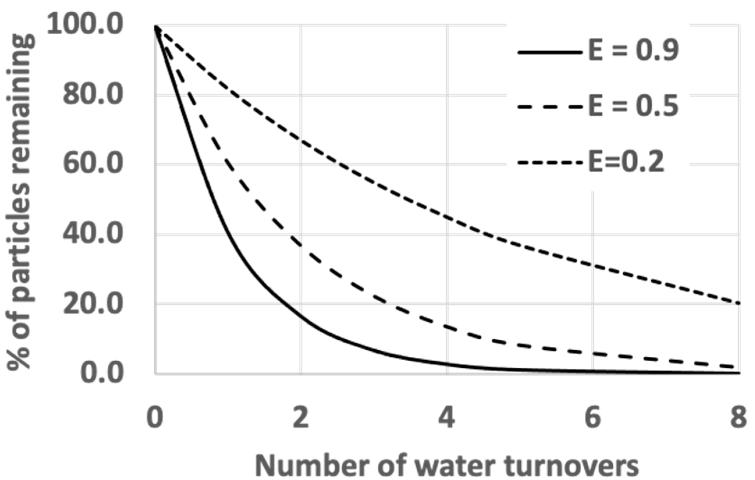
3.3. The Role of Filter Efficiency in Contaminant Removal

One application of the Gage–Bidwell Law of Dilution is to investigate the removal of Cryptosporidium oocysts from a well-mixed pool following an AFR. Though Cryptosporidium was not a known hazard in pools at that time, in the 1926 “Standards for design, construction, equipment and operation” the authors [9] did apply the Gage–Bidwell Law of Dilution to consider water purification in terms of the removal of dirt by filtration. The Gage and Bidwell abstract [9] stated that “It can readily be demonstrated by computation and by experiment that 7 turnovers are required to effect a removal of 99.9% of the dirt present in the water of the pool when recirculation was started. At the end of the first turnover the purification will be about 63%, after two turnovers about 86%, and after six turnovers 99.7%. To accomplish a purification of 99.99% 10 turnovers will be required”.

There is a clear legacy of this conclusion in the current guideline that six turnovers are needed to reduce the amount of Cryptosporidium oocysts remaining in the pool to an acceptable level following an AFR [6]. In this context, we can use Equation (8) to deduce that 99.7% of water would be treated in six turnovers, which would amount to 1.5 m³ of untreated water remaining in the case of a 500 m³ pool. As an example of the practical implications, this untreated water might still contain 300,000 oocysts if the pool is well-mixed and if there had been an input of 10⁸ oocysts prior to the six turnovers [17].

However, the analysis above is based on two assumptions: (a) the pool is perfectly mixed; and (b) the filters are removing 100% of dirt from water passing through the filter media. The Gage and Bidwell abstract acknowledged the latter and considered the consequence of filtration being less than 100% efficient. Following the imagined thinking of Gage and Bidwell, we can consider the effect of reduced filter efficiency by repeating the dilution experiment as shown in Table 1, but this time replacing only part of the water removed from the pool at each dilution with pure water (so that some fraction of the salts, or solids, in the water taken from the pool is returned to the pool).

Let the fraction of the water in each successive container that is replaced by pure water be termed E. This is analogous to the filter efficiency: a value of 1 represents a filter removal efficiency of 100%. So now we are not only removing the salts (or solids) present in volume 1/N at each dilution but are also returning (1 − E)/N back to the pool. Therefore, Equation (1), which describes the fraction remaining in the pool after one turnover, now becomes Equation (9):

$$\raisebox{1ex}{${\mathrm{C}}_{\mathrm{pv}}$}\!\left/ \!\raisebox{-1ex}{${\mathrm{C}}_0$}\right.=(1-\raisebox{1ex}{$1$}\!\left/ \!\raisebox{-1ex}{$\mathrm{N}$}\right.+{(1-\raisebox{1ex}{$\mathrm{E}$}\!\left/ \!\raisebox{-1ex}{$\mathrm{N}$}\right.)}^{\mathrm{N}}={(1-\raisebox{1ex}{$\mathrm{E}$}\!\left/ \!\raisebox{-1ex}{$\mathrm{N}$}\right.)}^{\mathrm{N}}$$

(9)

Following the same process that led to the derivation of Equation (3), this further leads to Equation (10):

$$\raisebox{1ex}{$\mathrm{C}$}\!\left/ \!\raisebox{-1ex}{${\mathrm{C}}_0$}\right.={\mathrm{e}}^{-\mathrm{ET}}$$

(10)

Figure 1 shows examples of how the time required for cleanup of particles (such as turbidity or Cryptosporidium oocysts) is extended if the filter efficiency is less than 100%. The selected examples range from E = 0.9, which corresponds to the value assumed by PWTAG [10] as the case for a well-managed pool, to E = 0.2, which Gregory [4] suggested to be a typical value for a pool with ineffective coagulation. This covers the range of efficiency reported by Lu and Amburgey [18] in a study of the impact of coagulants and filtration velocity on the removal of 4.5 µm polystyrene microspheres using sand filtration. The curves shown in Figure 1 accord with the statement made in the Gage and Bidwell abstract that “If the filters have an efficiency of only 50%, the effect will be the same as though the recirculation system were only half the size”. However, there have been very few studies on the efficiency of swimming pool filters in removing dirt (particles) in operational pools, so it is not widely appreciated that this is an aspect of the performance of pool water treatment that can be as important as the water-turnover time with respect to particle removal.

Given the importance of the combination of water-turnover time and filter efficiency in determining the rate of removal of particles from a pool, it is useful to combine these two parameters into a single key performance indicator that provides an overall measure of the effectiveness of the filtration system. Therefore, we propose the term ‘particle-turnover time’, T_p, as distinct from the water-turnover time, T_w = V/Q, given by Equation (11):

$${\mathrm{T}}_{\mathrm{p}}=\frac{\mathrm{V}}{\mathrm{QE}}=\frac{{\mathrm{T}}_{\mathrm{w}}}{\mathrm{E}}$$

(11)

where V is the pool volume (m³), Q is the circulation rate (m³ h⁻¹), and E is the fractional removal of either turbidity (NTU) or particles of a given size class from water in a single pass through the filter.

Whereas the turnover time for water (T_w) is the time it takes 63.2% of the water in a well-mixed pool to be removed, the particle-turnover time (T_p) is the time it takes 63.2% of particles to be removed. An example of this is illustrated later by diurnal measurements of turbidity (Section 3.5). There is an approximately exponential decrease in turbidity once the pool is closed, where the exponent is the particle-turnover time.

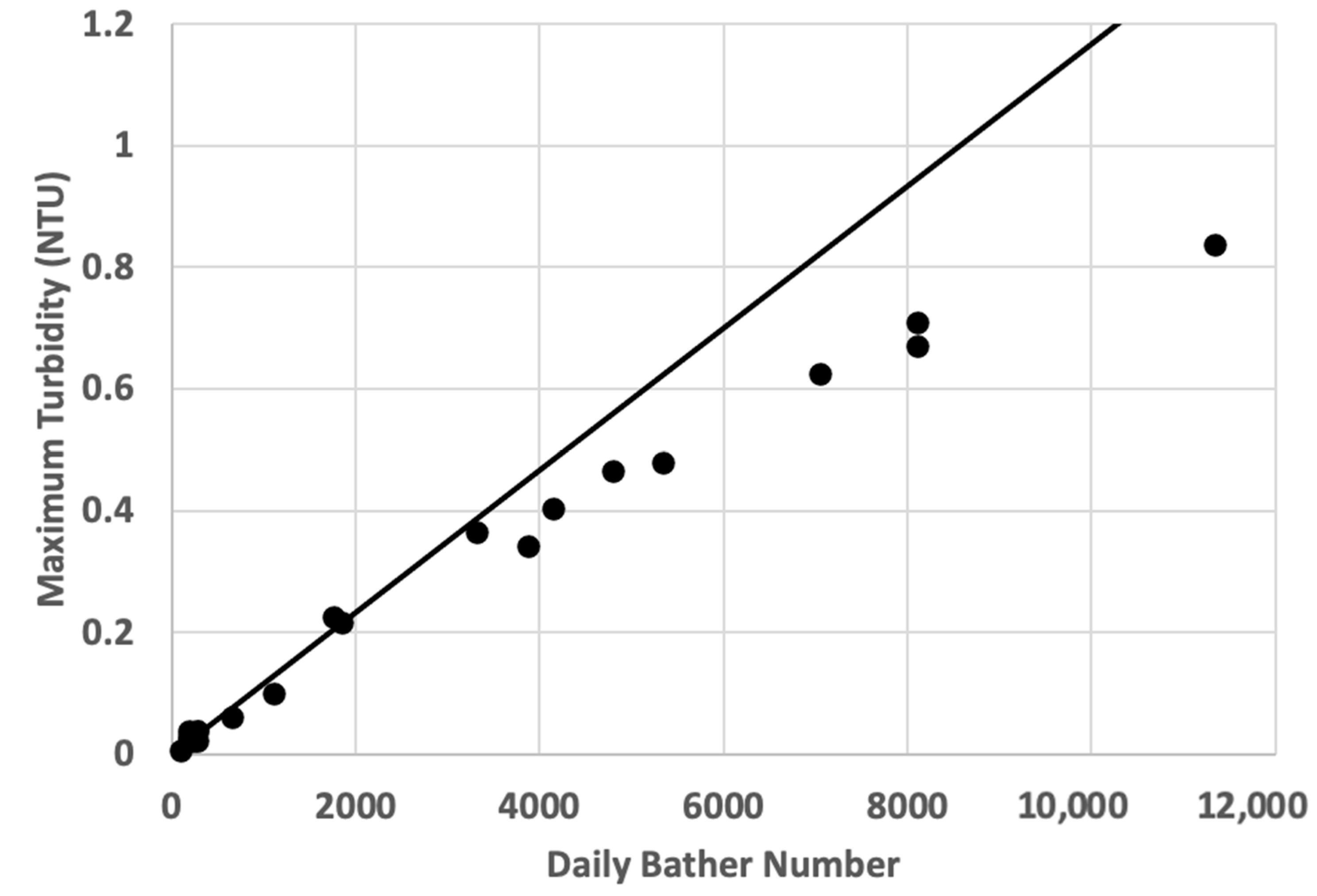
3.4. Application of the Gage–Bidwell Approach to Modelling the Peak Turbidity of Pool Water

So far, we have limited the discussion of the applications of the principles of the Gage and Bidwell abstract to the removal of a specific particulate material following a single contamination event (such as an AFR). We now consider the implications for the ongoing removal of a continuous input of a contaminant, and the dynamic equilibrium that exists between the input and the removal of a contaminant. We will explore this using the input and removal of turbidity from pool water. In this context, a key performance indicator of interest to a pool operator is the peak turbidity likely to be achieved. This has practical significance in managing the risk of a swimmer drowning, as it determines whether a lifeguard will be able to see the whole of the pool floor from a single point at poolside [6]. The prediction of the peak turbidity is complex, because it depends on highly variable factors that determine the temporal pattern of input of contaminants to the pool, which will depend primarily on the amount and distribution of bathing load throughout the day, and the nature and hygiene of the bathers [2].

An important concept introduced by Gage and Bidwell in their 1926 abstract [9] was that there will be some dynamic equilibrium between the rate at which turbidity (dirt) is added and the rate at which it is removed. In their words, “If the pool is used regularly by bathers further increments of dirt will be introduced into the water daily, and the removal of each successive daily increment will proceed according to the law. The result of the addition of such daily increments will be an increasing accumulation of dirt in the water up to a certain point, after which the dirt content of the pool water will remain practically constant. The amount of this accumulation depend[s] upon the rate of turnover of the pool and is also dependent upon the efficiency of the filters”. This simple concept of the ‘dirt content’ of pool water moving towards some equilibrium has rarely been applied to understanding the factors controlling the peak turbidity likely to be achieved in a pool at times of peak bathing load. Though it is beyond the scope of this paper to consider modelling the detailed time course of turbidity in relation to bathing load (as done by Stauder and Rodelsperger [13] using a differential continuity equation), we will show how the principles outlined by Gage and Bidwell [9] can be applied quite simply to achieve two things:

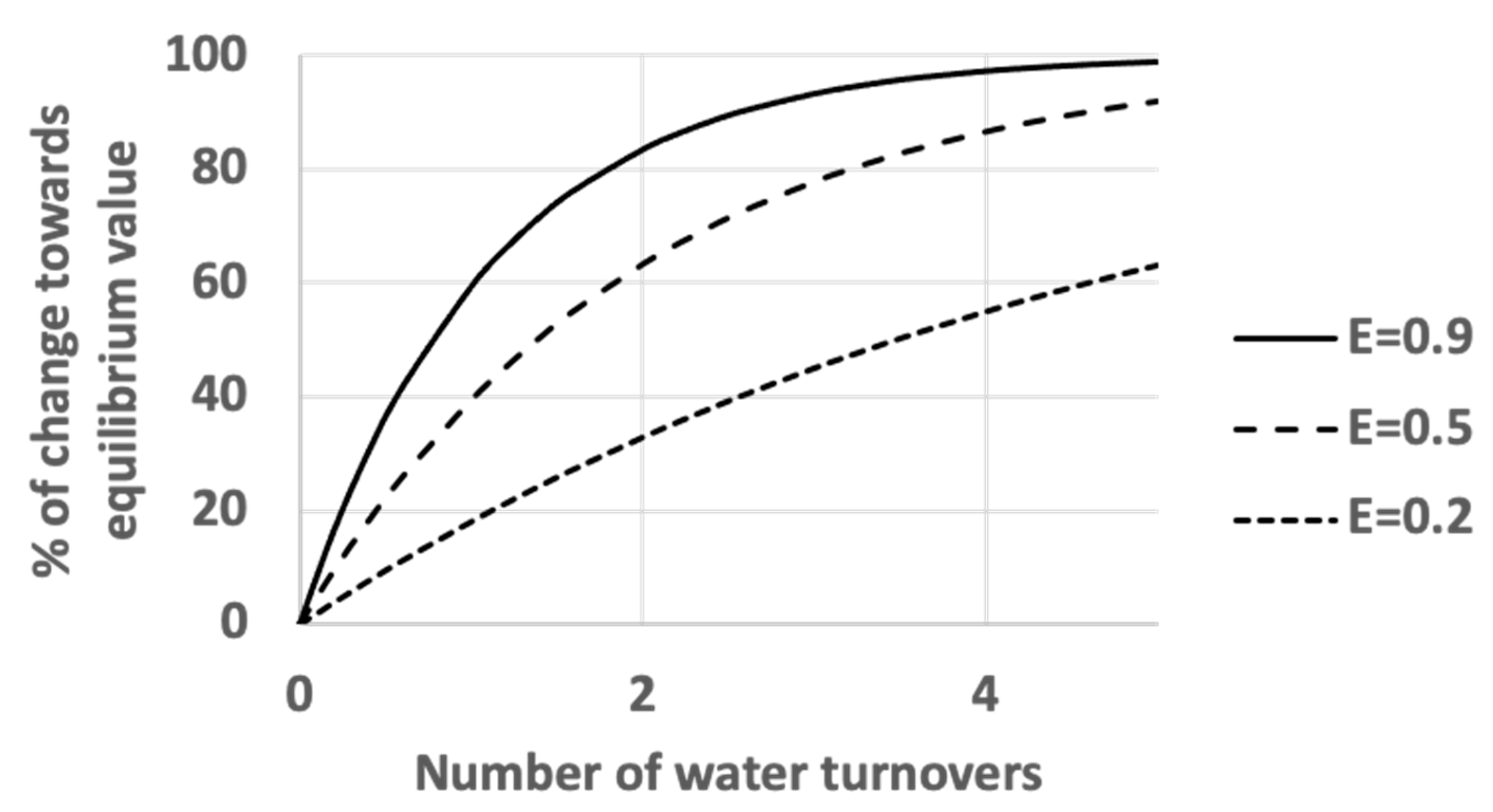
• To establish the equilibrium turbidity likely to be achieved if a constant bathing load (in terms of numbers of bathers per hour) is maintained indefinitely.
• To establish the maximum turbidity likely to be achieved if a constant bathing load is sustained for a finite time that is too short for the equilibrium to be achieved.

This provides a useful tool for assessing the performance of a pool in terms of the likely peak turbidity, and which could also be used to inform those responsible for developing guidelines for pool operation.

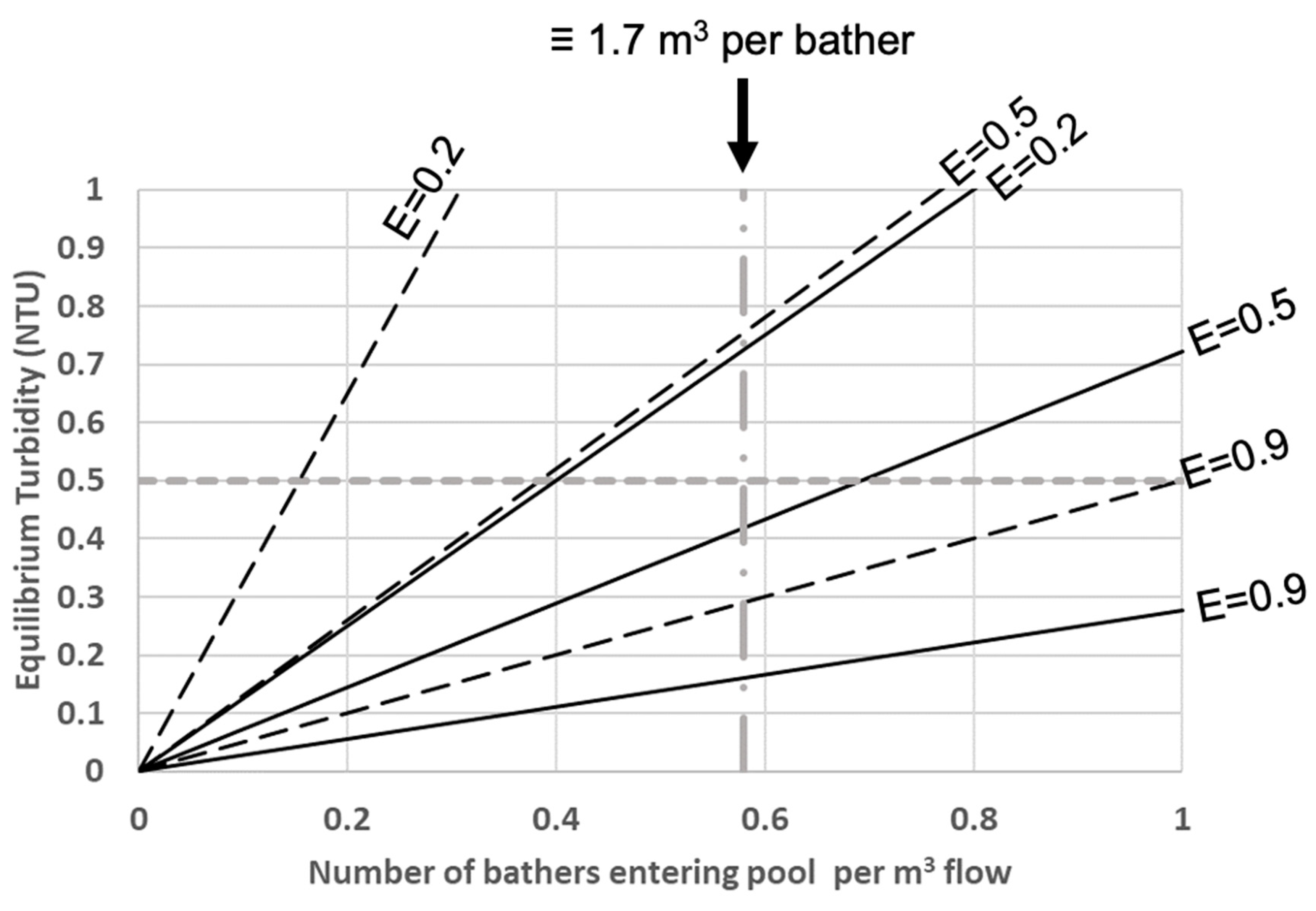
3.4.1. Modelling the Maximum Turbidity Achievable If the Design Maximum Bathing Load for a Pool Is Sustained Indefinitely

The principle stated by Gage and Bidwell in 1926 [9] using the term ‘dirt’, but applied here to turbidity, is that if a constant input of turbidity is maintained indefinitely, then the pool water turbidity will rise until the rate of removal of turbidity by filtration (which rises as the turbidity of water being delivered to the filter increases) matches the rate of input.

Turbidity is measured by nephelometry [6], based on the measurement of scattered light by particles in a sample, and expressed in units of nephelometric turbidity unit (NTU). The intensity of the scattered radiation is related to the intensity of the incident radiation and the concentration of particles that are causing the scattering [19]. In this analysis, we shall consider the turbidity of water expressed in NTU as a concentration resulting from the quantity of turbidity-forming particles introduced by bathers. Therefore, the rate at which turbidity is removed is equal to the product of the rate of delivery of turbidity-forming particles to the filter (i.e., the pool water NTU multiplied by the circulation rate, Q, in m³ h⁻¹) and the filter efficiency (expressed in terms of the fraction of turbidity that is removed in a single pass through the filter, E).

The hourly input of turbidity will be the product of the number of bathers entering the pool per hour (B) and the quantity of turbidity-forming particles added on average by each bather (K_p). If at equilibrium the rates of addition and removal of turbidity are equal, the equilibrium turbidity (C_e) is given as in Equation (12):

$${\mathrm{C}}_{\mathrm{e}}=\frac{{\mathrm{B} \mathrm{K}}_{\mathrm{p}}}{\mathrm{Q} \mathrm{E}}$$

(12)

In the analysis presented here, the values of B and Q are unequivocal, and the assumption is that they are kept constant. However, the values of K_p and E are more ambiguous and require further discussion.

The value of E depends on a number of factors, including the particle size [7], and would be expected to have a lower value if being used in the context of Cryptosporidium oocyst removal than for the removal of turbidity [7]. The value of E may also change with time, due to fluctuations during the course of a day (as the dirtiness of the water changes), and possible changes in performance of the filter media over periods of several days during the backwash cycle [20]. However, in the context of establishing the equilibrium turbidity during a period of constant bathing load the value of E for a filter would be expected to be relatively stable during the period that the equilibrium is being approached, assuming that other factors that affect the efficiency (e.g., coagulant dosing rate and the filtration velocity) remain constant.

In the context of turbidity, filtration efficiencies of 0.9 have been reported [13] for a pool with dual media anthracite/sand filters and coagulant (PAC) dosing optimised to minimise the measured filtrate turbidity. Where coagulation is poor or absent, filtration efficiencies of 0.2 (or less) are likely [4,18]. We shall examine the predicted equilibrium turbidity in scenarios used in Figure 1, where the filter efficiencies for turbidity removal during periods of protracted heavy bathing load will be E = 0.9, 0.5 or 0.2. This covers the range that most swimming pools are likely to be operating in.

There is little information on the likely values for the average amount of turbidity-forming material introduced per bather into pool water. Two approaches have been used to obtain this information. The first is to measure the rise in turbidity in a small body of water (e.g., a spa) following entry of by a known number of bathers, where the input per bather is calculated by dividing the rise in NTU by the number of contributing bathers per m³ of water. This method was used by Amburgey (personal communication, 2020) who reported an average K_p value of 0.65 NTU (bather m⁻³)⁻¹. A variation to this approach might be to collect shower water and measure the recovery of particles from individuals, as done by Keuten at al [21], although the range of values for the sloughing of turbidity-forming material was not reported. An alternative method was used by Stauder and Rodelsperger [13], who used the continuity form of Equation (10) to model the diurnal fluctuations in turbidity from the differences between the rates of input and removal of turbidity, based on the assumption of a well-mixed pool. The parameters affecting the modelled time course of turbidity were the circulation rate (Q), the filter efficiency (E), the known fluctuation in bathing load and the average K_p. As all parameters except K_p were known, values of K_p for each day were obtained by finding the values that gave the best fit between the modelled and measured time course of NTU. This resulted in values ranging from 0.25 to 0.5 NTU (bather m⁻³)⁻¹. However, it should be noted that Stauder and Rodelsperger [13] reported the daily visitor number, and it may be that not all the visitors entered the pool; therefore, these values will underestimate K_p. It should also be noted that as this was a paddling pool, not all bathers would be fully immersed, which is likely to reduce the inferred value for K_p. In the scenarios we consider below, we will use values of 0.25 or 0.65 NTU (bather m⁻³)⁻¹ to represent the range from ‘clean’ to ‘dirty’ bathers.

The application of Equation (12) as a guide for pool operators is illustrated by Figure 2, which shows values for the equilibrium (i.e., the maximum possible) turbidity for several pool scenarios. To facilitate a comparison between very different pools, the x-axis shows the ratio of the number of bathers entering the pool to the volume (m³) of water being treated (i.e., B/Q from Equation (12)). For example, a pool with 100 bathers h⁻¹ entering the pool with a water circulation rate of 200 m³ h⁻¹ would return a value of 0.5 bathers m⁻³ circulation, which is the same value as for a spa with 10 bathers h⁻¹ entering the spa with a water circulation rate of 20 m³ h⁻¹. To put the range of x-axis values into context, a leisure pool with an average depth of 1.5 m operating at maximum bathing load (allowing 4 m² water area per bather) and a 3 h water-turnover time would have a value of 0.5 bathers m⁻³ circulation.

The possible scenarios in Figure 2 also cover a range of filtration efficiency (E = 0.9, 0.5 or 0.2) [7]. These are shown in combination with relatively dirty or relatively clean bathers using K_p = 0.65 or 0.25 NTU (bather m⁻³)⁻¹ over the range of values on the x-axis likely to encompass most pools. With relatively good filtration (E = 0.9), the equilibrium turbidity value (achieved after a very long time of bathers entering the pool at a steady rate) will only just reach 0.5 NTU at a value of 1.0 bathers m⁻³ circulation with dirty bathers. However, pools with less effective filtration (E = 0.5) are at risk of the turbidity exceeding 0.5 NTU at a value of 0.5 bathers m⁻³ circulation when the bathers are dirty. Pools with relatively poor filtration (E = 0.2) are predicted to have excessive turbidity after prolonged periods of maximum bathing load at a value of 0.4 bathers m⁻³ circulation even with the cleanest bathers.

The concept of the number of bathers per m³ of water treated by filtration (x-axis Figure 2) is already established in pool operation guidelines. For example, the guidelines for pool operation in the UK [10] recommend that where the circulation rate is limited by the design of the pool, the maximum bathing load for the pool should be calculated from Equation (13):

Maximum bathing load (bathers per hour) = Q (m³ h⁻¹)/1.7

(13)

This value of 1.7 m³ circulation/bather is equivalent to an x-axis value in Figure 2 of 0.58 bathers m⁻³, shown by the vertical dashed line. Provided the filtration is relatively good (E = 0.9 in this case), this upper limit guideline maintains equilibrium turbidity of the pool water within an acceptable range (no more than 0.3 NTU even with very dirty bathers) in the case where the maximum bathing load is sustained indefinitely.

Note also that the model predicts that an upper limit guideline of 0.58 bathers m⁻³ (equivalent to 1.7 m³ water flow through the filtration system per bather) will result in only slight exceedance of the upper acceptable limit of 0.5 NTU, even with dirty bathers, i.e., K_p = 0.65 NTU (bather m⁻³)⁻¹, and relatively poor filtration (E = 0.5). In this respect, this guideline [10] is necessarily cautious in that it will maintain acceptable water quality even in pools with relatively dirty bathers and relatively poor filtration performance. Recommendations for water-turnover times for pools may also need some contingency for pools where the water volume behaves as a number of separate compartments and where the ratio of water circulation to bather number within a compartment could be rather less than the overall average for the pool.

3.4.2. Modelling the Maximum Turbidity Achievable If the Design Maximum Bathing Load for a Pool Is Sustained for a Finite Period

The preceding analysis considered the turbidity reached in swimming pool water when in a state of equilibrium achieved in the case where bathers continue to enter the pool indefinitely at a constant rate. This leads to the question whether bathing loads are ever sustained for long enough for the equilibrium turbidity to be achieved. For example, the measured diurnal courses of turbidity for the heavily used 690 m³ paddling pool studied by Stauder and Rodelsperger [13] showed large fluctuations in turbidity during the day, with the peak values generally appearing as sharp mid-afternoon spikes rather than approaching a plateau. This suggests that equilibrium turbidity values were a long way from being approached in this particular case.

Modelling using the Gage–Bidwell principles described above involves essentially the same problem as modelling the removal of Cryptosporidium oocysts following an AFR using Equation (10). The latter describes the transition from some initial concentration (C_o) to the special case of the final equilibrium concentration being zero. However, as we are now concerned with the accumulation of turbidity-causing particles from some initial starting condition (C_o) to a final non-zero equilibrium turbidity (C_e), Equation (10) can be written in the following more general form:

$$\frac{\mathrm{C}}{{\mathrm{C}}_{\mathrm{e}}-{\mathrm{C}}_{\mathrm{o}}}-{\mathrm{C}}_{\mathrm{o}}=1-{\mathrm{e}}^{-\mathrm{ET}}=1-{\mathrm{e}}^{-\mathrm{t}/{\mathrm{T}}_{\mathrm{p}}}$$

(14)

where the left side of Equation (14) represents the concentration of particles (or the NTU) expressed as a fraction of the step change from the original concentration (C_o) to the final equilibrium concentration C_e. Just as with the removal of Cryptosporidium oocysts, we see that after one particle-turnover time we have reached 63.2% of the final result of the step change and reached 99.7% of the change after six particle-turnovers.

Hence, the progress towards the equilibrium turbidity under conditions of constant bathing load is related to the number of particle-turnovers, irrespective of pool size. The implications are illustrated in Figure 3, which shows, for three filtration efficiencies, how rapidly the turbidity changes towards a new equilibrium value following a change in bathing load. For example, with relatively good filtration (E = 0.9), 90% of the change towards the new equilibrium turbidity occurs after 2.6 water-turnovers. Hence, for a spa with a 10 min water-turnover time, 90% of the transition towards the equilibrium NTU is predicted to be achieved in 26 min. This suggests that a spa is quite likely to approach the equilibrium NTU predicted for the maximum allowable bathing load. However, for a leisure pool with 1.5 m average-depth and 3 h water-turnover time, it would take 7.8 h of continuous maximum bathing load for the turbidity to reach 90% of the change from C_o to C_e. This explains why time courses of turbidity for leisure pools typically show short-term ‘spikes’ at times of peak bathing load, rather than approaching a plateau, because the fluctuations in bathing load are too rapid for equilibrium states to be approached.

If the filters were only removing 50% of the turbidity from water passing through the filters, the equilibrium turbidity would be higher, but the time taken to reach 90% of the change from C_o to C_e would increase to 47 min for the spa and 14 h of continuous bathing load for the pool. The implication is that in practice it is only in pools with very short water-turnover times (such as spas and paddling pools) that the turbidity is ever likely to approach the equilibrium value for the maximum instantaneous bathing load. Pools with water-turnover times longer than 2 h would not be expected to approach the equilibrium turbidity for the maximum bathing load that was used as the basis of the nomogram shown in Figure 2.

It should be noted that Figure 3 can also be applied to predict of the rate of reduction in turbidity during a recovery period when bathers are absent from the pool, and where the turbidity of the pool water will fall from its value at the start of the recovery period towards near zero. For example, using Equation (14), a heavily used water park pool with a 2 h particle-turnover would expect a 40% reduction in turbidity after just 1 h of recovery time, increasing to 63% and 78% removal of turbidity after 2 and 3 h, respectively. The implication is that for a pool with good filtration there is little benefit in terms of particle removal of recovery periods longer than a couple of turnovers.

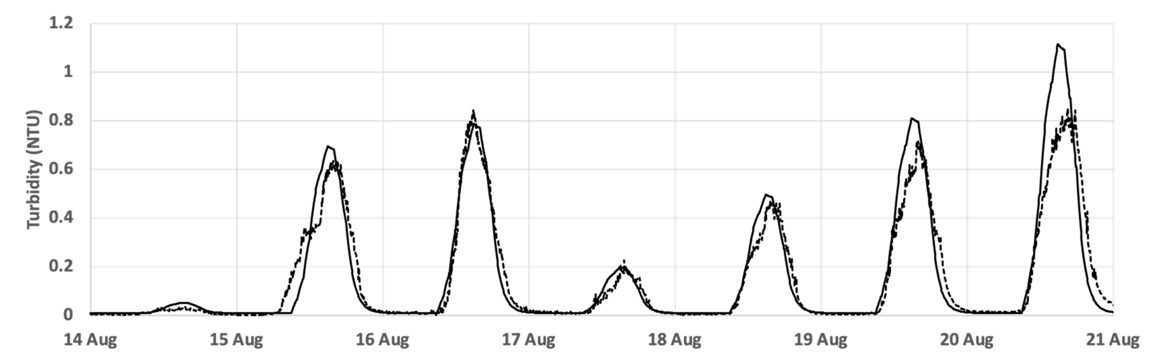
3.5. Modelling Observed Time Courses of NTU

Stauder and Rodelsperger [13] presented data showing the time course of turbidity over a 20-day period for a very busy outdoor paddling pool with large day-to-day variation in bather number. Stauder and Rodelsperger [13] also provided information on daily bather numbers (taken from their Figure 1), and so in order to model diurnal fluctuation in NTU we had to generate a bather frequency during the course of each day. To do this, we assumed that every day had the same time course of relative bathing load during the day, and that the relative bathing loads assigned to each hour period increased seven-fold from the first hour the pool opened to the period leading up to the time of peak turbidity. The temporal pattern of relative bathing loads was then scaled by the daily bather number to generate values for the numbers of bathers entering the pool during each hour.

The dashed line in Figure 4 shows the measured values of turbidity (NTU) during a week where there was a wide range of daily bather numbers. The data indicate that at night the turbidity values fall to <0.05 NTU, and then rise more or less steeply once the pool opens (depending on the bather numbers). The data indicate that generally a sharp peak occurs before the turbidity decreases once the bathing load falls, with turbidity decreasing particularly rapidly when the pool is closed.

The progress of turbidity (NTU) was modelled on an hourly basis using Equation (14) to predict the transitions in turbidity each hour. C_o was the turbidity value (NTU) at the end of the preceding hour, and C_e was calculated using Equation (12), based on the number of bathers entering the pool that hour and an assumed value for the turbidity input per bather. With a water-turnover time of 1.06 h and a filter efficiency of 0.9, Equation (14) predicts that in 1 h there will be 57% of the transition from C₀ to C_e. In this way the diurnal course of turbidity (NTU) was predicted, as shown by the solid line in Figure 4.

One key assumption made in this modelling exercise was that the temporal pattern of relative bather frequency was the same on all days. The second assumption was that the average turbidity (NTU) input per bather was the same at all times. This value was adjusted to optimise the fit of the modelled values to the measured values with the resulting ‘best fit’ value being 0.35 NTU (bather m⁻³)⁻¹. Despite these critical assumptions, the modelled time courses showed good agreement with the measured values and predicted the peak daily turbidity values to within 10%.

One of the purposes of carrying out these simulations was to predict the peak daily turbidity values for a pool and to compare them with the maximum observed values each day, to see whether this key performance indicator was predictable. Figure 5, based on the 21 consecutive days of data presented in Figure 1 of Stauder and Rodelsperger [13], shows the empirical relationship between daily bathing load and the measured peak turbidity values over a wide range of daily bather numbers. The observed peak turbidity (NTU) value was approximately proportional to bathing load. This would be expected if the days were similar in terms of the values of K_p, E, T_w and the temporal pattern of bather frequency, but differed only in the daily bather number, which would act to ‘scale’ the peak turbidity value.

The solid line in Figure 5 shows the equilibrium turbidity values that were predicted using Equation (12), corresponding to the peak mid-afternoon bathing loads. It is seen that the observed peak turbidity fell short of the equilibrium turbidity values, which is also indicated by the absence of any evident plateauing of turbidity (NTU) values during the busiest periods (Figure 4). However, because in this example the water-turnover time was relatively short (1.06 h) there were sufficient turnover times during the busiest periods for the peak turbidity (NTU) values to rise to >50% of the equilibrium turbidity values.

3.6. Public Health Implications

This paper has demonstrated a number of potential applications of a simple model of particle removal from swimming pools based on the underlying principles and assumptions in the Gage and Bidwell model of “water purification by consecutive dilution” (Gage–Bidwell Law of Dilution). These principles were originally presented as an early attempt to provide scientific underpinning to the design and operation of swimming pools [9]. Our paper has shown that such a relatively simple model can be used to identify the key performance indicators for assessing the effectiveness of pool filtration, and also to assist in the development of well-informed guidelines for pool designers and pool operators. Examples include:

• Prediction of the time it takes to achieve satisfactory removal of a contaminant (e.g., Cryptosporidium oocysts) following a single contamination event.
• Prediction of the maximum equilibrium concentration of a contaminant under conditions of a steady input of the contaminant (we considered the maximum turbidity achieved under conditions of a prolonged constant bathing load).
• Prediction of the amount of water that should be circulated per bather to ensure that water clarity remains excellent, even when there is a very prolonged period when bathers are entering the pool.
• Prediction of the peak turbidity likely to be achieved in practice from knowledge of the distribution of bathing load during the day.

All of these predictions depend critically on the water-turnover time (which is widely used as a key performance indicator for pools). However, also of importance is the filtration removal efficiency, a parameter which is rarely measured, and can vary widely in swimming pool filtration systems (e.g., [18]). Our analyses indicate very clearly that it is the combination of the water-turnover time (T_w) and the filtration efficiency (E) that provides the best overall key performance indicator of the effectiveness of filtration in swimming pools. We propose a formalisation of this concept in a new combined term, particle-turnover time (T_p = T_w/E), which could provide the basis for assessing the health and safety risks associated with particulate material in pool water. However, this requires the development of a practical methodology for assessing the effectiveness of filtration in operational pools, which is not generally available at present, but which might be based on the use of turbidity measurements or particle counting [7].

Another application of this modelling is to assess the extent to which recovery periods with no bathers contribute to the removal of the recently added ‘dirt’ from bathers. Analysis of the data in Figure 5 showed that by the time the pool was closed, 88% of the turbidity introduced by bathers had already been removed by filtration. This value increased to 93% and >97% at 1 and 3 h, respectively, after the pool had closed. This suggests that overnight recovery plays only a relatively small role in the removal of recently added dirt from bathers.

The shallow paddling pool studied by Stauder and Rodelsperger [13] was an extreme case of a pool with a very high bathing load relative to the pool volume. This provided an ideal data set for testing the Gage–Bidwell Law of Dilution in practice. Both the measurements and the modelling showed that even though the filters were very efficient, the 1.06 h water-turnover time was not sufficient to maintain the peak turbidity below the 0.5 NTU acceptable limit during days when there were more than 6000 bathers in the 690 m³ of water (Figure 5).

Consider now the case where the ratio of daily bather number to pool volume is more typical of a 25 m leisure pool, where the pool has the following attributes:

• Depth ranging from 1–2 m (average depth 1.5 m).
• 4 m² pool area allowed per bather at maximum bathing load following the UK guidelines [10], i.e., each bather occupies 6 m³ of water on average.
• 3 h water-turnover time.
• Average bathing time of 0.75 h.

If such a pool was operating continuously at maximum bathing load, then there would be 1.5 m³ of water treated per bather. This corresponds to a value of 0.67 bather m⁻³ for the x-axis of Figure 2, which would imply that with relatively good filtration of E = 0.9 [10] the maximum possible turbidity would be maintained below 0.4 NTU, even with relatively dirty bathers (0.65 NTU (bather m⁻³)⁻¹. With poorer filter efficiency (E = 0.5), the turbidity after very prolonged maximum bathing load would just exceed 0.6 NTU (i.e., slightly above the recommended upper limit) with relatively dirty bathers. With any reduction in the period of the maximum bathing load during each day (e.g., only two swim sessions, each of 3 h duration) the resulting maximum turbidity would be expected to be no more than 0.4 NTU.

3.7. Conclusions

We can conclude that, with the exception of pools with extensive shallow areas and long periods of near maximum bathing loads (based on UK guidelines), it would not be expected for leisure pools operating at near maximum bathing loads for prolonged periods to have water clarity issues due to any deficiency in the circulation/filtration system provided that (a) the filtration system is at least 90% efficient (E = 0.9) and (b) the water-turnover time was around the maximum recommended by industry guidelines [10]. With these conditions fulfilled, the above example shows that the maximum turbidity expected after 6 h of continuous maximum bathing load would be around no more than 0.4 NTU. There are indications [18] that filtration efficiencies in swimming pool filters can fall below the 90% values assumed in some of the treatment and quality standards [10]). However, there is a dearth of information on performance of filtration systems in operational pools. If, in practice, filtration efficiencies in swimming pools are much lower than this (which could be, for example, due to inadequate backwashing of filters or inadequate coagulation, insufficient filter depth, or excessively high filter loading rates), then this would be expected to cause water clarity to fall outside the acceptable range (as indicated in Figure 2). Though such a deficiency could perhaps be compensated for by increased turnover of water, it would be more appropriate to address any issues resulting in poor filtration, such as the effectiveness of the coagulation/filter aids, filter upgrades or the adequacy of backwashing procedures [7]. It should also be noted that establishing that the filtration is effective with respect to turbidity control does not necessary imply effective removal of Cryptosporidium, as the removal of particles the size of Cryptosporidium oocysts can be less effective than the sub-micron particles causing turbidity [7]. Furthermore, our model assumes irreversible removal by filtration and there is the possibility that previously-trapped oocysts may be released back into the pool (e.g., following backwashing) [2,7].

However, the principles discussed in this paper can be applied to the removal of Cryptosporidium, provided appropriate values for the filter removal efficiency are used. For example, we can assess whether the widely used recommendation [6,10] to close the pool to enable six turnover cycles following an AFR is reasonable (assuming an input of 10⁸ oocysts). If a filter efficiency for Cryptosporidium oocysts of 0.9 is assumed, as for example by PWTAG [10]), then Equation (10) predicts that after six water turnovers the concentration remaining would amount to 9000 m⁻³ in a 50 m³ pool, and 900 m⁻³ in a 500 m³ pool. Assuming that the average ingestion of pool water is 37 mL [7], the average ingestion of oocysts from pool water after 6 h of filtration would therefore be 0.3 and 0.03 oocysts in a 50 and 500 m³ pool, respectively. This is below the reported infective dose for Cryptosporidium [2,7]. However, if the filter efficiency is 0.5 or 0.2 (e.g., a sand filter with inadequate coagulation [4,18]), then a similar arithmetic leads to the conclusion that the numbers of oocysts ingested on average following six water turnovers increases in the case of the 50 m³ pool to 3.7 (E = 0.5) and 22.3 (E = 0.2) oocysts. This is within the range of the reported infective dose for Cryptosporidium [2,7] and suggests that in these cases six turnover cycles might be insufficient. This also raises the question of how filtration efficiency can be evaluated in pools [7].

The above is a simplistic exercise, and there is urgent need for more refined Quantitative Microbial Risk Assessment (QMRA) for Cryptosporidium. For example, the filtration modelling provides a sufficiently simple approach that can be used to incorporate filtration removal into the QMRA modelling, as recently developed by Falk et al. [22], but this is beyond the scope of this paper.

References

1. Lewis, L.; Chew, J.; Woodley, I.; Colbourne, J.; Pond, K. The application of computational fluid dynamics and small-scale physical models to assess the effects of operational practices on the risk to public health within large indoor swimming pools. J. Water Health 2015, 13, 939–952. [Google Scholar] [CrossRef] [PubMed] [Green Version]
2. Ryan, U.; Lawler, S.; Reid, S. Limiting swimming pool outbreaks of cryptosporidiosis–the roles of regulations, staff, patrons and research. J. Water Health 2017, 15, 1–16. [Google Scholar] [CrossRef] [PubMed]
3. Chalmers, R.M. Waterborne outbreaks of cryptosporidiosis. Ann. dell’Istituto Super Sanità 2012, 48, 429–446. Available online: https://www.iss.it/documents/20126/45616/ANN_12_04_10.pdf (accessed on 26 April 2021). [CrossRef] [PubMed]
4. Gregory, R. Bench-marking pool water treatment for coping with Cryptosporidium. J. Environ. Health Res. 2002, 1, 11–18. [Google Scholar]
5. Messner, M.J.; Chappell, C.L.; Okhuysen, P.C. Risk assessment for Cryptosporidium: A hierarchical Bayesian analysis of human dose response data. Water Res. 2001, 35, 3934–3940. [Google Scholar] [CrossRef]
6. World Health Organisation. Guidelines for Safe Recreational Water Environments. Volume 2: Swimming Pools and Similar Environments; World Health Organisation: Geneva, Switzerland, 2006; Available online: https://www.who.int/water_sanitation_health/publications/safe-recreational-water-guidelines-2/en/ (accessed on 26 April 2021).
7. Wood, M.; Simmonds, L.; MacAdam, J.; Hassard, F.; Jarvis, P.; Chalmers, R.M. Role of filtration in managing the risk from Cryptosporidium in commercial swimming pools—A review. J. Water Health 2019, 17, 357–370. [Google Scholar] [CrossRef] [PubMed]
8. Croll, B. Decontaminating swimming pools and managing Cryptosporidium. Recreation 2004, 2004, 32–35. Available online: https://poolsentry.co.uk/s/Croll-2004.pdf (accessed on 26 April 2021).
9. Gage, S.D.; Ferguson, H.F.; Gillespie, C.G.; Messer, R.; Tisdale, E.S.; Hinman, J.J., Jr.; Green, H.W. Swimming Pools and other Public Bathing Places. Am. J. Public Health 1926, 16, 1186–1201. Available online: https://ajph.aphapublications.org/doi/pdf/10.2105/AJPH.16.12.1186 (accessed on 26 April 2021). [CrossRef] [PubMed]
10. Pool Water Treatment Advisory Group. Code of Practice for Swimming Pool Water; Pool Water Treatment Advisory Group: Loughborough, UK, 2017; Available online: https://www.pwtag.org/code-of-practice/ (accessed on 26 April 2021).
11. Kanan, A.; Karanfil, T. Formation of disinfection by-products in indoor swimming pool water: The contribution from filling water natural organic matter and swimmer body fluids. Water Res. 2011, 45, 926–932. [Google Scholar] [CrossRef] [PubMed]
12. Ratajczak, K.; Pobudkowska, A. Pilot Test on Pre-Swim Hygiene as a Factor Limiting Trihalomethane Precursors in Pool Water by Reducing Organic Matter in an Operational Facility. Int. J. Environ. Res. Public Health 2020, 17, 7547. [Google Scholar] [CrossRef] [PubMed]
13. Stauder, S.; Rodelsperger, M. Filtration particles and turbidity in pool water. Removal by in line filtration and modelling of daily courses. In Proceedings of the Fourth International Conference Swimming Pool and Spa, Porto, Portugal, 15–18 March 2011; pp. 71–77. Available online: https://poolsentry.co.uk/s/Stauder-S-and-Rodelsperger-M-2011-filtration-particles-and-turbidity-in-pool-water-removal-by-in-lin.pdf (accessed on 26 April 2021).
14. Gordon, I.; Inglis, S. Great Lengths: The Historic Indoor Swimming Pools of Britain; English Heritage: Swindon, UK, 2009. [Google Scholar]
15. Alansari, A.; Amburgey, J.; Madding, N. 2018 A quantitative analysis of swimming pool recirculation system efficiency. J. Water Health 2018, 16, 449–459. [Google Scholar] [CrossRef] [PubMed] [Green Version]
16. Cloteaux, A.; Gérardin, F.; Midoux, N. Influence of swimming pool design on hydraulic behavior: A numerical and experimental study. Engineering 2013, 5, 511–524. [Google Scholar] [CrossRef] [Green Version]
17. Chappell, C.L.; Okhuysen, P.C.; Sterling, C.R.; DuPont, H.L. Cryptosporidium parvum: Intensity of infection and oocyst excretion patterns in healthy volunteers. J. Infect. Dis. 1996, 173, 232–236. [Google Scholar] [CrossRef] [PubMed] [Green Version]
18. Lu, P.; Amburgey, J.E. A pilot-scale study of Cryptosporidium-sized microsphere removals from swimming pools via sand filtration. J. Water Health 2016, 14, 109–120. [Google Scholar] [CrossRef] [PubMed] [Green Version]
19. Morais, I.P.; Tóth, I.V.; Rangel, A.O. Turbidimetric and nephelometric flow analysis: Concepts and applications. Spectrosc. Lett. 2006, 39, 547–579. [Google Scholar] [CrossRef]
20. Amburgey, J.E. Optimization of the extended terminal subfluidization wash (ETSW) filter backwashing procedure. Water Res. 2005, 39, 314–330. [Google Scholar] [CrossRef] [PubMed]
21. Keuten, M.G.A.; Schets, F.M.; Schijven, J.F.; Verberk, J.Q.J.C.; Van Dijk, J.C. Definition and quantification of initial anthropogenic pollutant release in swimming pools. Water Res. 2012, 46, 3682–3692. [Google Scholar] [CrossRef] [PubMed]
22. Falk, R.A.; Blatchley, E.R.; Kuechler, T.C.; Meyer, E.M.; Pickens, S.R.; Suppes, L.M. Assessing the Impact of Cyanuric Acid on Bather’s Risk of Gastrointestinal Illness at Swimming Pools. Water 2019, 11, 1314. [Google Scholar] [CrossRef] [Green Version]
Figure 1. Effect of filter efficiency (E) on the removal of dirt particles from pool water (expressed as percentage of particles remaining) following successive water-turnover cycles, based on the Gage–Bidwell Law of Dilution.
Water 13 02350 g001
Figure 2. Effect of the number of bathers entering the pool per unit volume of water flow through the filtration system on pool water equilibrium turbidity (NTU), assuming different dirt loadings per bather (solid line Kp = 0.25 NTU (bather m−3)−1; dashed line Kp = 0.65 NTU (bather m−3)−1) and different filtration efficiencies (E). The x-axis is the ratio of the number of bathers entering the pool to the volume (m3) of water flow through the filtration system (i.e., B/Q from Equation (12)) and value of 0.58 is equivalent to 1.7 m3 water flow through the filtration system per bather.
Water 13 02350 g002
Figure 3. Effect of filtration efficiency (E) on the rate at which turbidity approaches equilibrium following a change in bathing load as the number of water-turnovers increases.
Water 13 02350 g003
Figure 4. Comparison of the measured time course of turbidity (NTU) (dashed line) over 7 days with the prediction (solid line) made using Equations (12) and (14) and with values of Kp = 0.35 NTU (bather m−3)−1, Tw = 1.06 h, and E = 0.9. The number of bathers entering the pool each hour was derived from the recorded daily bather numbers, and an assumed frequency distribution during the opening hours. Based on data of Stauder and Rodelsperger [13].
Water 13 02350 g004
Figure 5. Empirical relationship between daily bathing load and the measured peak turbidity (NTU) over a wide range of daily bather numbers, based on the 21 consecutive days of data presented in Figure 1 of Stauder and Rodelsperger [13]. The solid line shows the comparison with the peak turbidity if the turbidity was at equilibrium with the peak bathing load (Equation (12)).
Water 13 02350 g005