
Developing the Food, Water, and Energy Nexus for Food and Energy Scenarios with the World Trade Model


1
ARAID (Aragonese Agency for Research and Development) Researcher, Agrifood Institute of Aragon (IA2), Department of Economic Analysis, Faculty of Economics and Business Studies University of Zaragoza, Gran Vía, 2-50005 Zaragoza, Spain
2
Department of Mechanics and Mechatronics, Institute of Space Technologies of Academy of Engineering, Peoples’ Friendship University of Russia (RUDN), 117198 Moscow, Russia
*
Author to whom correspondence should be addressed.
Water 2021, 13(17), 2354; https://doi.org/10.3390/w13172354
Submission received: 23 June 2021
/
Revised: 22 August 2021
/
Accepted: 23 August 2021
/
Published: 27 August 2021
(This article belongs to the Special Issue Water Footprint and Virtual Water Trade Approaches: Applications to the Water-Energy-Food-Land Nexus in a Context of Climate Change)
Abstract
:The food, energy, and water (FEW) nexus has gained increased attention, resulting in numerous studies on management approaches. Themes of resource use, and their subsequent scarcity and economic rents, which are within the application domain of the World Trade Model, are ripe for study, with the continuing development of forward- and backward-facing economic data. Scenarios of future food and energy demand, relating to supply chains, as well as direct and indirect resource uses, are modelled in this paper. While it is possible to generate a substantial number of economic and environmental scenarios, our focus is on the development of an overarching approach involving a range of scenarios. We intend to establish a benchmark of possibilities in the context of the debates surrounding the Paris Climate Agreement (COP21) and the Green New Deal. Our approach draws heavily from the existing literature on international agreements and targets, notably that of COP21, whose application we associate with the Shared Socioeconomic Pathway (SSP). Relevant factor uses and scarcity rent increases are found and localized, e.g., on the optimal qualities of water, minerals, and land. A clear policy implication is that, in all scenarios, processes of energy transition, raw material use reduction, and recycling must be strengthened.
1. Introduction
The food, energy, and water (FEW) nexus has gained increased attention, resulting in numerous studies on management approaches [1,2]. According to the United Nations’ (UN) estimates, the population of the Earth will approach 10 billion by 2050 (World Population Prospects 2019) [3]. In this context, it is crucial to emphasise the increasing demand for food, energy, and water (FEW) and the variety of severe challenges expected to arise to satisfy those fundamental demands. The World Economic Forum notes that a major source of uncertainty for the global economy is clearly aligned with other developments and claims, such as that of [4]: “The Implementation of the 2030 Agenda requires a more holistic, coherent and integrated approach at the national, regional and global levels”. Many studies have discussed the concepts of the FEW nexus and modelled certain relationships, although not many have studied the additional implications holistically. Progress has been made in recognizing and quantifying those demands, developing new approaches to the management of scarcity, and projecting them into the future [1,2,5]. Surmounting the challenges is possible only if a transdisciplinary approach is used, establishing sustainable supply chains that are managed from the FEW nexus [6] and developing a multidisciplinary approach in the form of a “web”, rather than a “linear tree” [7].
Within the vast FEW related body of work including social science methods, we highlight those addressing the relation with the economy and global trade, in particular with input–output methods and exploring scenarios. We utilize the literature review in [8] as a starting point to comprehend FEW related works. Accordingly, from the tabulation and categorization of FEW nexus tools and methods from all 73 ‘methodological’ papers, 25 (34%) were classified as scenario analysis, and 33 (45%) as economic studies. Of those the closer to ours in methods were the two of value chain analysis, the three of Supply chain analysis, the 10 of Tradeoff analysis and especially some of the 15 (20%) of the classified “input–output analysis” or social accounting matrix, which are also often paired with scenario assessment. Three articles that were classified as IO were [9,10,11] because they work with input and outputs of the models. However, we note that we would not classify them as input–output analyses since they do not use actual IO tables or/and models. There were eight studies that indeed worked with input–output models, and actually dealt with FEW nexus challenges (even if not making them explicit) [12,13,14,15,16,17,18,19,20].
Our model extends from this literature on the FEW with IO, and links the energy and food with the water system, which has been a central piece in most of the FEW related work. One of the most important reasons is probably that although the interactions go in many directions, water is, for example, key for food production (while the opposite link is not relevant). In the interaction with energy the link is more balanced (e.g., energy is needed for water processing, treatment, pumping, desalination…), but water scarcity is very often highlighted as a major constraint to socio-economic development and a threat to livelihood in increasing parts of the world [21], also due to energy needs such as the growing attention to China’s water security concerns due to the combustion industry [22,23,24]. We make a strong emphasis in the modelling of water by: (a) highlighting and modelling the importance of the water input to the other dimensions of the nexus and other sectors, with different water quality types; (b) representing and modelling different water qualities, which can or cannot be used depending on the sector (e.g., some can use only high quality forms); (c) incorporating knowledge on the actual available endowments, which in the case of water need to take into account environmental requirements; (d) being these endowments endogenously modified based on the capacity of performing water treatment by each region (based on their technological status); (e) this is the result of the modelling of water treatment sectors, and a water distribution sector (which distributes to the sectors in the economy both taking the water input from and nature and from those treatment sectors).
As highlighted in [2,25], an array of challenges exists in relation to the data—and knowledge gaps—of the FEW interlinkages, as well as to the shortage of systematic tools to address the synergies and trade-offs in the nexus domain. Water, food, and energy are all managed in various, and often very different, spatial and temporal scales, which often make comparisons difficult. In this case we tried to focus all of them together in the most common types of scenarios, and projections (for 2050). The cited articles underlie the importance that assumptions and system boundaries of the various nexus dimensions are made very clear. With our unified IO framework, the whole consistency of accounting equally for inputs and outputs across them, avoiding double counting and with full world supply-chain system boundaries, is clear. They also note that the challenge of including water quality has been identified as one of the key weaknesses of global water assessments [21] and so we provide the assessment of different water qualities, which can or cannot be used depending on the sector, and furthermore whose endowment is endogenously modified based on the capacity of performing water treatment by each region (based on their technological status). Similarly, it is highlighted [2] that nexus studies are prone to include only some components in electricity generation, e.g., through hydropower dams often the most relevant (and even only) form of energy. Here we incorporate this, but also the water needs of energy (coal, gas, nuclear… and energy needs of the water sectors), as their interrelation with other sectors. The gap of attention being given to the inclusion of emissions of the energy sector in the FEW studies is also solved here, by explicitly including and accounting for the GHG emissions and imposing modelling constraints according to climate policy.
Reference [25] also notes the FEW nexus touches on a broad range of stakeholder interests, visible in the Sustainable Development Goals (SDGs) of the United Nations. Water, energy, and food are present individually and in combination in most, if not all, of the SDGs, although nexus-based approaches are not explicitly included in those goals per se—for example, food (SDG 2), water (SDG 6), energy (SDG 7), climate (SDG 13), resource efficiency (SDGs 8 and 12), and life on land (SDG 15). Quantifying the complicated interdependencies among these factors is critical to achieving these goals [26].
In the context of SDGs and resource use, a wide range of scenarios have been designed and tested to evaluate different futures using numerous models across many disciplines. Global climate change activists have developed a scenario framework to analyse future impacts and policies [27,28], and various analyses have been proposed [29,30,31,32]. Shared Socio-economic Pathways (SSPs) provide a flexible framework for local scenario development, that can be used in adaptation and vulnerability studies. Specifically, a global narrative storyline has been developed for SSPs that incorporates aspects of demography, economics, land use, human development, technology, and environment [33,34,35,36], all of which are of relevance to this study.
We generate an input–output (IO) model to address the FEW-based implementation of scenarios with the SSP narratives. Multidisciplinary and multisectoral work on IO and hybrid LCA (Life cycle assessment)-IO analyses address many of the challenges cited above, broadening the system boundaries by incorporating the socioeconomic and environmental aspects of FEW dimensions, and by extending their scope and functionality [12,13,14]. In [37] a transnational inter-regional input–output approach was applied to analyze the FEW nexus in East Asia. The authors showed a mismatch between regional food-energy-water availability and final resource consumption, with significant requirements in the People’s Republic of China (from now on, China) in terms of pollution and resource use to satisfy the demands of Japan and South Korea [37].
Specifically, we find that a linear programming IO, and the World Trade Model (WTM) [38] with the Rectangular Choice of Technology (RCOT) is ideally suited to accommodate socioeconomic and environmental information and results related to FEW, in terms of global and regional production, demand, trade, resources, and their scarcity, along with other relevant variables. The WTM has proven to be a useful model, not only to study trade flows, but also to explore population needs and pressures on FEW under different scenarios, both for the present and the future [15,17,39]. For example, the evaluation of future changes in population, income, food demand, agricultural yields, and energy transitions have been successfully studied by the WTM. The model enables endogenous choices of geographical regions and technologies to produce commodities and services, and simultaneously calculates resource uses and rents (from scarcity) not only for the classical factors of production (labor and capital), but also natural resources such as water [17,40,41].
The primary objective of this article is to shed light on the implications of the different narratives described in the literature, with a special focus on food and energy projections, to generate insights into production according to comparative advantage, trade, factor uses, notably water, and scarcity rents. To accomplish this, we use cross-sector data to identify and model feedbacks, not only between the sectors in the center of the hydrological, energy and food systems, but also in the rest of the economy. This allows us to capture macro level information that would not be available using a model targeting a FEW-only domain. Our secondary objective is to put these results into context by juxtaposing them with key studies of resource and material uses and scarcity projections (e.g., [42,43,44,45,46,47]). Third, we extend the discussion of the utility of these results to complement insights into virtual water and water footprints [48,49] and show modelling that overcomes some of the usual critiques and related discussions [50,51,52,53,54,55,56,57], by implementing a comprehensive framework from a multiregional, multisectoral, and multifactorial perspective.
The remainder of the article is organized as follows: Section 2 presents the WTM, the data, the properties, and extensions of this work. Section 3 presents the scenarios to be analyzed, mainly consisting of using different coherent narratives projecting key variables. Section 4 presents our main results, combining those on the different paths effects on production, trade, factor uses, and scarcity rents. Section 5 extends the discussion, and summarizes the main conclusions, implications, and possible future work. The Supplementary Material contains extensions on the methods, scenario assumptions, and additional results. On the methods, we provide Tables with details of variables, sectors, and regions, as well as equations of the dual model. Scenario descriptions provide additional details, especially on the FEW, demographics, and income projections.
2. Methods: The WTM
This section is in four parts.
Section 2.1 reviews the WTM/RCOT literature
Section 2.2 presents our WTM/RCOT model.
Section 2.3 describes the Database used, detailing data sources.
Section 2.4 illustrates with a diagram how each component works together.
2.1. The WTM/RCOT Literature
The WTM has been instrumental in developing and analyzing scenarios of global production, trade, consumption, technologies, environmental threats, use and endowment of resources, and constraints. WTM-based studies have shed light on the economic and environmental implications stemming from challenges of food, energy, and water security. These studies may comprise what-if scenarios [20,39,40,41,58,59], but also cover projections for the future given increasing demands [15,18], and for strictly regional analyses [39,40,58,60] or global scale analyses [18,20,41]. The present work aims to combine the relevant drivers and features of existing studies, by considering the food, energy, and water (FEW) nexus in a context in which these needs can be satisfied.
2.2. The WTM/RCOT Model
We present the WTM/RCOT as a simple model with high explanatory power. Making use of the parameter and variables (see Table S1 in the Supplementary Material), the primal model takes the following form:
subject to
The primal model in Equation (1), minimizes the total factor use cost in monetary terms, using linear programming. In particular, the use of factors of production per unit of output in region I , times their factor prices in the region , times the sectoral output in region i . Equation (2) ensures that production is sufficient to meet the final demand , making use of the inter-industry inputs per unit of output in region i (this is obtained by dividing the multiregional IO table by the sectoral output). Equation (3) ensures that factor use does not exceed the available factor endowments . Equation (4) ensures that production is non-negative in each region. Equation (5) is the benefit-of-trade constraint to ensure trade is preferable, by requiring that the value of exports be less than the value of imports at no trade prices that are calculated in a separate solution, where each region has to meet its own final demand without factor constraints.
The dual model and the extension of the WTM with Bilateral Trade (WTMBT) are presented in the Supplementary Material (first section) in more detail. This last feature provides more realism to the present solutions, which is emphasized by introducing additional constraints on the security needs (e.g., a certain share of production of a region needs to be produced domestically, constraining the equation with ), where is a value between 0 and 1 for the sector in question (e.g., for barely traded services).
We incorporate the feature of the Bilateral Trade in our modelling, which transforms Equation (2) into Equation (6):
matrix specifies the requirements of transporting a good from region j to i. The output is the sum of intermediate production requirements , exports net of imports, , transport demand required for carrying imports and regional final demand . The WTMBT, with , captures costs of transport, and allows the introduction of additional import tariffs. I. Although we want to keep working with a “purer” representation of comparative advantage among regions (i.e., no constraining factors more than realistically to obtain a more accurate/matched baseline solution), the feature of Bilateral trade reduces the cases of very skewed solutions (e.g., only one country producing all of a product). is a composite of the matrix, which represents the weights of goods for each transport mode, the interregional distances and the on the “easiness of trade”, with values around 1 depending on the extra barriers or facilitation of trade for regional clusters and trade associations (e.g., USMCA for US, Mexico and Canada, Mercosur for Latin American countries, etc.):
Scenarios may differ, but we retain for the future the structure of , and the scale is only increased when there is a more-rivalry scenario, in which it is envisaged that international relations have deteriorated.
2.3. The Database
One novelty here is to identify and model the feedback web between food, energy, and hydrological systems. Input–output and factor matrices try to specifically represent key accounts for food, energy and water, which requires additional data that are not ordinarily available in IO databases. Technological changes are allowed by having multiple technologies “competing” as simultaneous options. This is the case of agricultural, electricity, and water treatment and distribution sectors, but also in some others, such as motor vehicles, for which an alternative technology of electric vehicles is introduced (using [61,62,63]).
Within the present WTM-RCOT database, (as shown in Table S2), we work with 16 technologies of crop production (eight crops, with two irrigated/dryland production for each); eight electricity technology options, and three water technologies (one for water distribution and two for water treatment technologies), building further on the developments in [18,20,41] with a database developed from GTAP9. The disaggregation of the original energy and water sectors in GTAP is based on the EXIOBASE database [64,65], implying a disaggregation in the A matrices, but also factor uses, which had not been considered earlier, such as, for example, the land requirements of technologies such as solar [66] (apart from those of biomass or hydro).
A more accurate representation of water use from electricity technologies is another novelty. Efficiency changes are introduced in key sectors, such as agriculture, electricity (e.g., the impact of ‘smart grids’ on electrical efficiency is expected to be large) and water treatment and distribution. Several studies have recently provided further information on this, such as on the consumptive WF per unit of electricity output for different energy sources per stage of production (see [67], which also contains a literature summary on the impact of electricity from different energy sources, [40,68]).
Since the model is quite capable of capturing differences in technologies, factor use, and endowments among countries, there are now 19 regions (Table S3), based on a compromise of accounting for different socioeconomics, physical conditions, and endowments.
Regarding the discussion of [69] on the different implications of how factors are dealt with in the model, here they are defined mostly as being shared across technologies. There are few cases of an association of a single technology and factor (a technology-specific factor): the technology of fishing, the technology of forestry, and those of extraction of minerals, coal, oil, and gas.
Finally, while previous WTM/RCOT (except for [15]) scenarios had a narrower focus, here we adopt a more holistic and comprehensive approach to capture possible feedback mechanisms and non-linear relationships that would not be possible in a focused study. Our scenarios incorporate a wider range of possible paths, using projections and data from disparate sources on changes in population, wealth, diet, energy and water demands, resource use and availability, and technological change.
2.4. Modelling, Scenarios, and Results Framework
The diagram below (Figure 1) illustrates how each of the components of the article work together. As a starting point, the SDGs developed by the UN provide a motivation for this FEW article, which develops its own version of these scenarios based on the data that can be processed by the World Trade Model. This scenario development requires data from a number of disparate sources, their processing, standardization, and harmonization via statistical and geographic aggregation and disaggregation methods. After the economic database is complete, the economic model subject to its properties is run to obtain the necessary endogenous variables, which are the results of this paper.
3. Future Scenarios
Studies have shown that the extent of climate change impacts largely depend on assumptions made about socio-economic conditions [35,70,71]. Others have argued that applying different socio-economic scenarios is more effective than applying different climate change scenarios [72,73,74]. In this context, the global research community has developed Shared Socio-economic Pathways (SSPs), which provide a flexible framework for local scenario development, with quantitative and qualitative descriptions, that can be used in adaptation and vulnerability studies. Additionally, a global narrative storyline has developed for SSPs in demography, economics, land use, human development, technology, and environment [33,34,35,36].
We follow this approach (scaled for different geographical and sectoral applications [75], and regularly revised given the challenges it faces [76]), although we recognize that there are other possible approaches, e.g., those more focused on specific aspects of green growth, degrowth, equity, more radical social policies, certain technological visions, better reflection of the role of competition, relative scarcity of resources, climate change dynamics, and so on (see e.g., [77,78,79,80]).
Accordingly, our study consists of five general scenarios based on the SSPs
- (1)
- SSP1 “Sustainability”, taking the green road, the only one which, in principle, does not pose challenges for mitigation and adaptation;
- (2)
- SSP2 is the “middle of the road” scenario;
- (3)
- SSP3, which assumes an aging society, increased income “inequality” between classes and regions, the resource-intensive industrial structure, and slow economic development resulting in environmental degradation;
- (4)
- SSP4, “Regional rivalry”, with large socio-economic challenges for adaptation;
- (5)
- SSP5, “Fossil-fuel development”, which assumes very high GDP and urbanization growth, with a clear inverted-U shaped curve for population growth, revealing a demographic transition.
In our results, we focus more on the ones that we see are more active in the world today: SSP2 “middle of the road”, and SSP3 “inequality”. We do not present results on SSP4 “Regional rivalry”, given the uncertainty about the possible effects of regional rivalries. SSP1 “Sustainability” seems to embody the aspirations of certain global agreements, but based on too many indicators that are still evolving, as is SSP5 “Fossil-fuel development”, based on the economies of fossil fuels in regions such as the European Union.
As we introduce in the following Section 3.1, we have tried to unify the data on Gross Regional Product and population projections obtained mainly from the SSP Database Version 2.0 and United Nations. This allows us to project future final demand. Furthermore, in order to project the final demand for food (addressed in Section 3.2.1), water (Section 3.2.2), and energy (Section 3.2.3), we model the changes in the technologies producing them (e.g., yield improvements, see Section 3.3), which also affects the rest of the economy for each scenario. Although there could also be alternatives to the assumptions made, we have chosen to retain current country/regional trade associations and clusters.
3.1. General Scenario Framework SSPs
At the Paris Convention, nations agreed that it was necessary to stabilize the temperature increase at less than 2 °C [81]. For decades, researchers have argued that the global temperature rise must be kept below 2 °C above pre-industrial levels, by the end of this century, to avoid the worst impacts, but scientists now agree that keeping below 1.5 °C is a far safer limit for the world. The mitigation burden varies with the SSP; SSP3 “inequality” requires ambitious mitigation policies with higher costs, including rigorous international emissions trading, use of advanced low-carbon technology such as fuel cells, and a higher renewable energy supply rate, although SSP1 is the one that we associate with accomplishing the 1.5 °C target.
As we see below in Table 1, major proxies for each sector are identified through the review of SSP studies [29,82]. These are basically based on past trends and future projections. Most of the SSP data provides info at 5-year steps, so we linearly interpolate to run the model in shorter timesteps. Additionally, although the baseline year is 2015, we run the model for the first years for the known final demand percentage changes.
Further explanation of this framework as well as the practical implementation in the model of demographics and income changes is presented in the Supplementary Material (Section 3.1, including Figure S1: Relation of forcing levels (climate scenarios) and SSPs, including carbon prices and Figure S2: SSPs situation in terms of challenges for adaptation and mitigation).
3.2. Future Food, Water, and Energy Demand
3.2.1. Food Demand
Understanding the capacity of agricultural systems to feed the world population under climate change requires some elaboration and projection of future food demand. Valin et al. (2014) note that the underlying drivers of food demand are subject to uncertainty; demographics are not easily predictable beyond a few decades, and economic growth is even less predictable. To account for such uncertainties and for the wide range of possibilities, the authors compared 10 global economic models (participating in the Agricultural Model Intercomparison and Improvement Project, AgMIP) to provide projections of future agricultural market conditions, under common scenarios [83]. Food demand projections for 2050—with a world population of almost 10 billion people—for various regions and agricultural products were compared under harmonized scenarios of socioeconomic development, climate change, and bioenergy expansion. As for the SSPs in IIASA, the authors provide data for different regions and scenarios, so that we can project SSPs accordingly. Their reference scenario (SSP2) had an average increase of 74% in terms of calories, as opposed to the 54% projected by FAO [86]. The range of results is large, in particular for animal calories (between 61% and 144%), caused by differences in demand systems and in income and price elasticities. The results are more sensitive to socioeconomic assumptions than to climate change or bioenergy scenarios. In general, all of the projected scenarios from 2005 to 2050 show about 70% growth of food demand. When considering a world with higher population and lower economic growth (SSP3 “inequality”), consumption per capita declines, on average, by 9% for crops and 18% for livestock. The maximum effect of climate change on calorie availability is −6% at the global level, and the effect of biofuel production on calorie availability is even smaller.
We develop a range of future demands for food for these different scenarios, changing the final demands of each region based on the work of Valin et al. (2014) [83]. The general relation among regions (Table S3) and crops (Table S4) is the one shown in the Supplementary Material. Specific country/region changes are especially studied for SSP2 and SSP3 “inequality”, along with an average of scenarios 3 to 6 on RCP 8.5. We also examine the results for an average of all 10 models.
3.2.2. Agricultural Yields and Water Use
Changes in final demand are complemented with the technology changes in the input–output matrix. We complement the information from the SSPs from IIASA (yield) with the yield changes from [90]. A linear interpolation from the baseline year (2015) to the 2050 projections is performed in order to study the entire temporal range annually.
According to [45], crop yields would continue to grow through the year 2060 but at a slower rate than in the past. This process of decelerating growth has been underway for some time and annual growth over the projection period would be about half (0.8% in developing countries) of its historical growth rate, i.e., 0.9% (2.1% for developing countries). Cereal yield growth would slow down to 0.7% per year (0.8% in developing countries), and average cereal yield would reach some 4.3 tonne/ha, up from 3.2 tonne/ha at present, by 2050.
3.2.3. Energy
Figure S3 shows the overview of basic SSPs in relation to the energy sector. We also explore and use, as an alternative scenario, the International Energy Outlook (2019), and in particular the World total final energy consumption by region, as a baseline increase of final demand [91]. Final energy consumption is the total energy consumed by end users and by the energy sector itself. In [84], their Figure 2 shows the final energy demand by SSP, with narratives of energy as described in the Supplementary Material (subsection on Energy for scenarios assumptions).
We also acquired information on electricity generation from both the SSP scenarios and the EIA [85] as an output for the WTM, and we consider the potential technological changes over the years, as described in the Supplementary Material (subsection on Energy for scenarios assumptions and Table S5 on relative cost estimates in 2030 and 2050 with respect to 2050).
Regarding the practical implementation of the WTM, we project the evolution of these specific technologies mainly with changes in the technical coefficients (A), and also in the factor use coefficients (F), when some information is provided. Specifically—and importantly for the nexus—we project, the development of renewable energy from wastewater, with reuse of methane in the agribusiness sector (and others), which only large companies are currently applying. This is apart from commonplace aspects, such as the water needs of electricity generation, or the energy requirements of modernized irrigation. Future energy savings will come, for example, from solar energy for purification in water treatment plants. In the food sector, notably beverage production, given the relatively high energy cost of biological treatments for wastewater, combinations of biological processes and non-biological processes (such as advanced oxidation) are progressively introduced. An increase in second-generation biofuels, reducing demand for food feedstocks, is also expected. By 2050, certain alternative technologies (for example, lab-grown meat) may ease supply constraints, although this is difficult to model, and so general improvements and technological changes are applied without trying to guess the cost structure of those disruptive technologies.
Regarding endowments, the baseline constraint for the fuel factors (as mining, etc.) is based on the concept of reserves (recoverable with at least 90% probability), and the constraints are relaxed over time as a function of the available resource, following the concept of ultimately recoverable resources [87].
3.3. Technological Change and Variables for the Rest of the Economy
Together, income convergence, structural change, and technology development are projected to lead to a relative decoupling of primary materials use globally. Unless large rebound effects occur, technology improvements should reduce future materials use per unit of production, in all major sectors of the economy, albeit at widely varying rates, as shown in Figure 4 of [45]. According to that study, material intensity per unit of output is projected to decrease through 2060 by a significant margin (around 30%), while more modest reductions (5–20%) in intensity are expected in the food sector, electricity and utilities, agriculture, and other manufacturing. These data are interpolated to obtain values for 2030 and 2050 in our A matrices. This does not impede higher material use in the simulations, since economic growth, increasing affluence, and/or different patterns of consumption may compensate for possible reductions from structural and technological change. As Ref. [44] summarizes, studies modelling the transition to a circular economy provide assumptions regarding average material productivity improvements, for which the baseline typically is the closest to SSP2. Most economies must further strengthen all processes reducing raw material use, recycling, etc., under any possible scenario.
All in all, there are many sectors for which we may not easily project technical change, which is associated with changes in total factor productivity. In [88] four scenarios for the year 2050 were analyzed, with a “business as usual” or baseline scenario projecting future rates of GDP growth of 3% per year, and yield improvements of 0.35% to 1% per year. As shown in Table 2 of [89], medium growth is projected for 3 SSPs, low growth for SSP3 “inequality”, and high growth for SSP5 “Fossil-fuel development”. Fast convergence among regions is found in SSP5 “Fossil-fuel development” and also in SSP1.
4. Results
4.1. General Trends
The interplay among all exogenous variables and parameters generates a large set of endogenous results for each designed scenario. The point of departure between scenarios includes a set of key aspects, mainly food and energy demands, yield changes, and energy technologies. This is the key to the FEW nexus. The differentiated results, based on standardized, literature-based scenarios provide comparable insights into the nexus from a new point of view.
Although specialization does occur, several countries produce goods for each technology, given the relatively high disaggregation for input–output studies, especially in some technologies, such as agriculture or electricity production, although they remain lacking in detail. The increasing role of China in the Global Value Chain (GVC) is captured, both in supply and demand in traditional trade, and other recently changed geographic dynamics, with a greater density of cross-border interactions [92,93], large volumes of trade, and some clear-cut trade “clusters” and hubs.
In general, we have seen in recent decades an unprecedented demand for raw materials, notably driven by the rapid industrialization of developing countries. Consumption of raw materials doubled in three decades (since the early 80s) and projections are that this use will continue to grow in the next three decades by an additional 30%. Materials intensity is projected to decline the most in China and India, where the infrastructure boom is coming to an end. In the 2010s, construction minerals accounted for the lion’s share of extraction (more than 50%), while biomass and fossil fuels represented about 20% each (the rest being minerals and ores). Relating these data to the economic sectors in the model, it is clear that land, water, and mineral-based fertilizers are critical inputs to food production, which—as shown in one of the most critical scenarios, SSP3 “inequality”—still have important increases, in a first period more related to cereals and rice, and a second phase more connected with meat.
Oil, coal, and natural gas dominate the current energy mix in many countries, but this is expected to change over time, especially in the more sustainable scenarios. Iron, for steel, and non-metallic minerals, for cement, are still essential in construction and infrastructure development, as is bauxite that is transformed into aluminum for the transport sectors.
However, the resources generating further constraints, due to present and estimated future physical availability, are less clear. Such constraints have to do more with the costs of extraction and hence factor prices, cost of transport, etc. Furthermore, although we have results for certain minerals and other materials that are fundamental for many construction and industrial activities, here we focus more on the direct food and energy transitions that are built into the scenarios we designed.
Generally, our results are consistent with the UNEP International Resource Panel [94], which projected that total resource use may more than double by 2050 if existing trends continue (the most similar to SSP2). According to [95], unless resource efficiency is significantly improved, this is likely to lead to increasing input costs and, for some resources, a growing risk of supply shortages.
As is projected for 2050 in [46], most of the growth in crop production derives from higher yields and increased cropping intensity, with the remainder coming from land expansion. Almost all the land expansion in developing countries would take place in Africa and South America.
Up to 2030, the projected trend in the emergent or developing countries is much more one of acceleration of both economic activity and materials use, with less room for decoupling. From then on, this process occurs particularly in China (also considering that in the plans developed for the Paris agreement peak emissions are expected in 2030), followed by India, then in other economies that are often called “emerging” or “emergent”.
As an example of the reflected technological change, even under the scenario with more conflicts in this regard, SSP3 “inequality”, we obtain Figure S4, showing a nearly 0% production of electric vehicles in 2015, to around 30% in 2030 and almost 100% in 2050. (Note: the model has some tendency to provide skewed solutions if a lower cost technology exists with available resources).
In the following we describe more specific results by key aspects of the nexus and their interactions (e.g., water uses are still largely driven by agriculture, so that the main constraints for the sector have to do with water and land), focusing particularly on comparisons between countries and resources.
4.2. Agriculture, Water and Land
Given the described future food, water, and energy demand, we next examine different sectoral productions and resource uses that will be affected. Agricultural production is an example of a sector where the projection changes can clearly be seen, with notable implications for the use, scarcity, and rents of water and agricultural land. The baseline scenario provides clear-cut specializations that are consistent with the reality of world production and trade. Noticeable examples are:
- –
- India especially in sugar, vegetables and fruits, wheat and some other crops;
- –
- The EU, particularly in cereals;
- –
- China, and other Asian regions, in rice production.
Of those, Japan and Korea produce some cereals, Malaysia and Indonesia produce oil seeds and a few other crops. Further, vegetables and fruits are produced across many regions, and exhaustion of resources implies having several producers at the same time, as occurs for all agricultural production, notably the Americas, African regions, and India. Plant-based fibers are produced in the Middle East and North Africa (16MEAS_NAF_RSA) and South Asia. Scarcity rents are accrued even for low quality water in India, China, Southeast Asia, and to some extent in Brazil (it should be remembered that the “inaccessible”/”impractical” water resources are not accounted for in the endowments), 16MEAS_NAF_RSA, Other, Eastern Europe and West Asia (region18, see Table S3), and in Japan, Korea, and Europe. Scarcity rents in higher quality water depend much more on other water uses (e.g., for electronic equipment) and are found, apart from most of those regions cited above, notably in Japan and Korea.
Scenario SSP3 “inequality” implies some regional rivalries, affecting trade among countries/regions, showing pressures on local water resources and land, and changes in agricultural production result (Figure 2), with the WTM/RCOT based on comparative advantage for SSP3 “inequality”. Agriculture is progressively domestic, and this affects water scarcity in regions such as Japan, Korea, China, the EU, and the UK, exhibiting short-run pressures from increased wheat production. The water footprints from production increase notably in China, Japan, and Korea, while virtual water exports are reduced globally, particularly in Canada, India, South and Central Africa, Central and South America, Malaysia, and Indonesia.
We suspect that if the global economy moves in the direction of further resource optimization and cost efficiencies, it will likely happen at the expense of further increases in water stress at certain locations, which are increasingly specialized as they have the comparative advantage of agricultural production. While the stresses may be less severe in the real world, due to the inefficiencies and redundancies of agricultural production, we are confident that the model demonstrates the trends. Although we expect that localized water stress and shortages will be more common, we anticipate that technological advances in irrigation will also evolve. However, we do not yet incorporate a paradigm change just yet and we remain cautious in our projections.
Harvested irrigated land is also projected to expand, according to our results, at around 15% in the whole period in SSP2, mostly from increases in developing countries, and the regions of South and Central Africa, South America, Central America and India, in particular. The Global Agro-Ecological Zone study shows that there are still ample land resources with some potential for crop production, but this result must be strongly qualified. According to the study, much of the suitable land not yet in use is concentrated in a few countries in Latin America and sub-Saharan Africa, i.e., not necessarily where it is most needed, and much of it is suitable only for certain crops that are not necessarily the crops for which there is the greatest demand [46]. In our model, land factor constraints exist for Middle East and North Africa, South Asia (region 7, see Table S3), and Rest of South East Asia (region 5). Even more concerning is that, even under the most favorable, sustainable scenario (SSP1), the solution entails some important requirements. Apart from the significant increases in built-up land, this is also true for certain minerals and, to some extent, for fish, water, and land needs.
In general, much of the land not yet in use suffers from constraints (chemical, physical, endemic diseases, lack of infrastructure, etc.) which cannot easily be overcome or is not economically viable, as indicated by [46]. Pastureland use also increases between 10% in SSP1 and 30% in (SP5, with around 20% in the other scenarios by 2050.
The increase in water use is not, in general, as high as land use changes, with around 15% by 2050 in the medium scenario of SSP2, including the negative water returns provided by the water treatment sector in this total. This obviously is indirectly reflected in energy use. When we set aside the water treatment sector and returns of water to higher quality forms, we find that total water use increases by up to 70%.
The availability of freshwater resources shows a very similar picture to that of land availability, i.e., globally more than sufficient, but very unevenly distributed, with an increasing number of countries (or regions within countries) reaching alarming levels of water scarcity. This is often the case in the same countries in the Near East/North Africa and South Asia that have no remaining land resources. One mitigating factor could be that there are still ample opportunities to increase water use efficiency (e.g., through providing incentives to conserve water), increasing water reuse, or using water treatment technologies in the most threatened regions. Figure 3 shows all the factor use changes from 2015 to 2050 with the WTM/RCOT for SSP1.
4.3. Electricity Production
Our model does not impose any growth in consumption or production of electricity, just technological options, changes, and factor constraints. Despite this, our model indicates that the share of renewables in energy supplies will grow dramatically. Without constraining the model, the pure WTM solution sees a dominant position for the production of electricity from wind. Most countries will produce up to 70% of their electricity from wind by 2050. Furthermore, on the two technologies of vehicle production, the 2015 solution provides for vehicles from the traditional non-electric technology, by 2030 the production is mixed, and in 2050 it is all electric. This process appears to be regionally localized, but given that we do not assume a particularly better technology in one place than in the other, this result is simply dependent on how world production and trade is organized, through specialization and resource availability. The production of electric vehicles is dependent on more inputs from electronic components and fewer inputs from other sectors. The solution to the production of electricity technologies of the WTM/RCOT at the 2015, 2030, and 2050 timesteps is shown below.
Figure 4 shows, on the one hand, that despite having projections of the requirements for each type of energy, by having a single sector and choice of technologies with the RCOT, the model, as presented, selects technologies according to costs, resource availability, and specialization. Despite that the model allows very skewed (due to specialization) solutions, to a large extent, and this is relatively consistent with [47].
In 2015, renewables provided 7% of China’s total final energy use. Under the renewable energy roadmap (REmap) case prepared by IRENA, this share increases to 67% by 2050 (to 60% in our SSP1 scenario, with almost 95% being in the electricity mix). In the European Union, the share could grow from about 17% to over 70% according to REmap, while our study achieves 75%. In 2015, renewables accounted for 36% of India’s final energy use, one of the highest shares in the G20 countries. However, when traditional use of bioenergy is excluded, its share of modern renewables is only around 10%. Under the REmap Case of IRENA, India would increase its share of modern renewables to 73% by 2050, while our calculations result in 68% for India and up to 60% for the USA.
4.4. GHG Emissions
Regarding GHG emissions, we impose constraints according to climate policy. SSP1 requires very high prices on carbon; in our results, more than USD 100 per unit of measure in 2030 and USD 500 in 2050, in order to have a feasible solution to the problem. A recent report from the OECD [96] found that the average carbon price across 42 major economies was around USD 8 per ton in 2018, far below the level most experts say is necessary to address climate change. According to [97], those low prices may reflect political constraints on pricing carbon directly. In Figure S1, we see carbon prices of [35] in terms of the net present value (NPV) of the global average, from 2010 to 2100 (using a discount rate of 5%). SSP2 would imply an average carbon price of USD 10/tCO2 (range: USD 10–USD 110/tCO2). Focused on a shorter period, the Stern-Stiglitz report set out USD 40–USD 80/tCO2e by 2020 and USD 50–USD 100/tCO2e by 2030. Additionally, ref. [98] estimated that a global tax of USD 75 per ton by the year 2030 could limit the planet’s warming to 2 °C. However, a later UN report estimated that governments would need to impose effective carbon prices of USD 135 to USD 5500 per ton of carbon dioxide pollution by 2030 to keep overall global warming below 1.5 °C.
Under most other SSPs, scarcity rents from GHG emissions, reflecting the “cost of pollution” based on a carbon tax, reveal a very high global cost (but also rents earned in the first years) of pollution, depending on the levels of activity and the energy transition. For example, in particular under SSP5 “Fossil-fuel development”, scarcity rents (the rents associated with pollution) of GHG reach the highest levels, together with the scarcity rents of minerals. This is in line with [45], which stated that more than half of all greenhouse gas (GHG) emissions are related to materials management activities.
- Fossil fuel use and the production of iron and steel and construction materials lead to large energy-related emissions of greenhouse gases and air pollutants;
- Metals extraction and use have a wide range of polluting consequences, including toxic effects on humans and ecosystems;
- The extraction and use of primary (raw) materials are much more polluting than secondary (recycled) materials.
In this line, metals are the materials (in our model) whose use is projected to grow the fastest (metal ores at around 70%), with copper and nickel having the largest environmental impacts. Non-metallic minerals, such as construction materials, are projected to grow rapidly (from around a 50% rate in SSP1 up to almost 100% in SSP5 “Fossil-fuel development”).
In our results, scarcity rents for copper go up significantly. Furthermore, although not fine-tuned in our database, critical and rare minerals are often by-products of larger mineral processes, such as copper extraction, so in the coming years the availability of some of these will also depend on its price.
As a limitation, we point out that we have grouped certain minerals that may be scarce in the future into an aggregate factor. More specifically, Table 2 summarizes the main results of scenarios, in terms of our focus on FEW.
Billen et al. (2015) studied equitable diets whose animal protein content does not exceed 40%, suggesting that it would be possible to feed the projected global population of 2050 with larger volumes of interregional trade, with higher nitrogen contamination, despite some efficiency gains. In our work, we find additional results for this scenario, showing the changes in land, water, and other factor requirements [99].
As is illustrated in [45], in our SSP2 scenario the general increase in global material use lies between the percentage increases in population (lower bound) and income per capita (higher bound). For SSP3 “inequality”, we see the greatest pressures on land and water. In particular, Japan presents strong constraints, finding in the case of SSP3 “inequality” outstandingly high scarcity rents of land and water towards 2050, even when the water treatment sector almost doubles in volume. Something similar occurs for the Middle East, and even for the EU, whose higher level of development of agriculture increases these pressures.
5. Discussion
Global demand for materials has increased 10-fold since the beginning of the 20th century and is set to double again by 2030, compared to 2010, according to [100]. It is recognized (e.g., [101]) that if present trends continue, human demands on the Earth’s ecosystem are projected to exceed nature’s capacity to regenerate by close to 100% by 2030—meaning that we would need two Earth-sized planets to meet human demands.
In this context, water footprints and virtual water studies have also shown how pressures directly and indirectly occur across frontiers, with previously unrecognized global forces at work driving local-scale problems [48,49,102,103,104], as well as challenges and measures of water scarcity not solely focused on blue water (surface- and groundwater), but also on green water (soil moisture directly returning to the atmosphere as evaporation; see [105]) and grey water studies [106,107,108].
Some authors have questioned whether policy solutions based on water footprints and virtual water concepts may be myopic (or not realistic) by not considering the interrelation of other factors in the socioeconomic choices of production location, trade, and policy. This article overcomes some of those critiques and related discussions around the policy implications obtained, by developing a comprehensive framework, with multiregional and multisectoral data, as well as multifactorial data (water, but also land, minerals, etc.), which allows us to obtain results accounting for such uses, for endowments, and for scarcity rents. In particular, our baseline solution highlights major low-cost producers in each production sector—India especially in sugar, vegetables and fruits (together with several American and African regions), Asian regions in rice production, Malaysia and Indonesia in oil seeds, the EU particularly in cereals, the Middle East, North Africa, and South Asia in plant-based fibers, and so on.
Under a middle-of-the-road scenario, SSP2, water use increases are not projected to be as high as land use changes, with around 15% up to 2050, which includes endogenous water returns (hence with possibilities of reuse) provided by the water treatment sector. Under SSP3 “inequality”, which recent events and decisions have made less improbable, agriculture is progressively domestic, and this affects water scarcity in regions such as Japan, Korea, China, Europe, and the UK, with short-run pressures from the increase in wheat production in China, the EU, and the UK. Water footprints of production are increased, notably in China, Japan, and Korea, while virtual water exports are reduced globally, especially in Canada, India, South and Central Africa, Central and South America, Malaysia, and Indonesia.
Our results can be contrasted with other studies which tend to find a much larger portion of the population that is exposed to increased water resources stress in some, if not all the future scenarios they investigated [29,70,71,73]. The reason for this fundamental departure is the nature of the models utilized across these studies, including ours. The contrasted studies utilize spatially explicit models that are fed primarily future climate data. Whereas, in our application the World Trade Model has two main mechanisms to address the scarcity of resources. The first one is the utilization of trade, which assures the transfer of water from water abundant regions to water scarce regions in the form of virtual water, which is the water embodied in the production of food and non-food commodities. The second mechanism is the extensive use of wastewater treatment technologies we implemented in all the economic regions we studied, which provide virtually unlimited amount of reusable water, with the inclusion of a price tag. Finally, the spatially explicit models and our approach differ in the resolution of the data we incorporate. Our approach requires us to work with much larger geographical units of study, while the spatially explicit models incorporate high resolution grid data with much ease.
An energy transition is projected among most studies and scenarios, even though some narratives, e.g., SSP1, project faster changes than others, e.g., SSP3 “inequality”. Still, the resource needs are limiting in all cases, with high scarcity rents (in the case of SSP1, e.g., through carbon tax constraints to maintain low levels of GHG) and even greater growth in narratives of economy and population (e.g., SSP3 “inequality” and SSP5 “Fossil-fuel development”). The competition for certain raw materials will increase in the future as key countries such as China and USA, together with the EU, are all highly reliant on imports of the same materials. Interestingly, despite the different possible transitions to a circular economy providing assumptions regarding average material productivity improvements, all scenarios incorporate some forms of energy transition and deployment of green technologies. Being aware that many technological developments, material use and cost reduction per unit produced, etc. have been historically often underestimated (even envisaging scarcity or polluting crisis that latter on did not occur, see [109]), especially due to the energy transitions the scenarios imply some raw materials scarcity and material bottlenecks in the future development of green technologies (see on this [110]).
A clear policy implication is then that, in all scenarios, processes of energy transition, raw material use reduction, and recycling must be strengthened. Most economies must further strengthen all processes of raw material use reduction, recycling, etc., under any scenario, given the low departing point in terms of circularity, mostly driven by the fact that processed materials are used to provide energy, not available for recycling [111]. As summarized in [44], circular economy roadmaps were introduced in China in 2013 (with the objective of reusing industrial solid waste), in the EU in 2015, and later in other countries. Examples of policy frameworks related to resource efficiency or materials management are Japan’s Fundamental Law for Establishing a Sound Material-Cycle Society, and the Sustainable Materials Management Program Strategic Plan in the USA. The latter includes a national target of a 50% reduction in food waste by 2030 [112]. Such frameworks are being established with the idea that there are many interlinkages in policies and potential benefits among the associated economic, environmental, and social aspects.
Our results reveal that feasibility of SSP1 is only possible under a combination of reduced demand, a fast energy transition, and important technological advances that will reduce the requirements of inputs per unit of production. Furthermore, as discussed around the Green New Deal for the last decade [113,114,115,116,117], and now dominating the media scene as a set of proposals for the post-COVID19 crisis, significant investments, involving infrastructure and needs from the material base, are required. Even under these scenarios, important initial requirements that impede direct reductions in factor uses, show—at best—an inverted-U shape.
At the company and sectoral levels, in sectors such as agriculture, food industry, and water treatment, the technologies present trade-offs between the quality of water obtained, the energy used, and their costs. This is reflected in the choices of the WTM/RCOT, and so with the global minimization of factor costs, dominant technologies are selected based on their production recipes (dependent on their technological costs), resource use, and availability.
As discussed and summarized by [118], resource-scarce countries need to re-consider their economic development patterns if they want to have food and environmental security.
In terms of the limitations of this work, we can point to the following. First, the inherent uncertainty of the scenarios for the future leads to uncertain results, limited to ranges. By taking different narratives and paths, we have tried to minimize this, but still these should be taken as what they are, possible futures dependent on several hypotheses. Second, in order to build our model, we have tried to unify the information on projections, mainly from the IIASA database, but taking data from different sources is unavoidable, especially when we are attempting to cover so many different aspects: economic accounts and trade, resource uses and bases, different possible futures, etc. We have tried to frame those projections within the SSP narratives, but again there has been subjectivity of interpretation of each SSP.
Aspects of the FEW nexus that are not specifically modelled could be improved in future work. For example, we have accommodated two technologies of vehicle production, in which the production of electric vehicles is dependent on greater input from electronic components and less from other accounts. However, in terms of consumption, we could not properly capture the introduction of hydrogen produced from renewable electricity as a vehicle fuel, since we did not have an associated technology factor; all we can see is higher consumption of electricity and less of oil.
Related to these concerns, we do not fully capture the scarcity of very particular minerals. Rare metals are especially vital for renewable energy technologies, such as electric cars (a Tesla vehicle, for example, requires about a bowling ball’s worth of lithium) and photovoltaic panels need the rare mineral tellurium. Other so-called rare earth metals, and the more traditional copper, uranium, and gold, are critical due to their properties and may see spiking prices because of their important role in the production of weapons, computers, batteries, smartphones, and other electronics. Returning to the electric vehicles discussion, e.g., on how the cost of batteries may go down (100USD /kWh is a current “magic number”, where EVs and gas-fueled vehicles reach retail price parity, which was in 650USD /kWh in 2009 and seems to have been reached, [119]), we could not properly link the global demand for lithium batteries, which is expected to rise sharply [61].
Future work may focus more on these other aspects, which ultimately are another nexus in a complex society, with multiple networks and interlinkages among socioeconomic factors and the physical base. Another line of future work is that of interlinking which policies could facilitate a move from one SSP to another, and how these could contribute to mitigation and adaptation processes, not to mention concerns of vulnerability and exposure to natural disasters, infrastructure deterioration, vulnerable population, and so on. As for technological changes, adaptation and mitigation policies affect many sectors (notably industry, construction, and energy) and should guide optimal decision-making.
On these aspects a text such as [109] about how fast things have changed in the recent history (especially compared to earlier periods) on technology, more speculative about future scenarios, etc., one may become more optimistic. Or at least, more convinced about the technical possibilities, and actually of the accomplishment of such changes, partly with political will (which at some places such as the EU seems to be more present than ever), but also partly simply due to technological and market transitions (e.g., as the taking over of renewable energies over fossil-fuels due to technological development and cost reduction, which, together with other limits that global environmental change may impose, probably make less likely mainly fossil-fuel-based societies as it has occurred until very recently). Related key examples have to do with how some technologies have (and others similarly could be) deployed also in the so-called developing world (with enormous potential for energy transitions e.g., of distributed generation such as solar, as it occurred with the mobile technology adoption).
On the other hand, we find radiographies of the evils and dangers that afflict contemporary society, e.g., [120], critiques to techno-optimism [121], and Refs. [122,123] highlighted even more the urgency of global changing action, which has been discussed strongly since the early 90s, with the Kyoto protocol, etc. Looking at all the graphs on how GHG emissions have increased in the XXth and early XXIst centuries, and how they should go inversely down (showing a sharp bell shape type) even in some not surely safe paths, one gets an intuition of the very large policy (perhaps forms of global governance) and behavioral changes that are needed. Overcoming some considered failures (e.g., [124]) and inertias (at the individual level through ‘habits’, and at the level of socio-technical systems) to improve energy and climate policies has been largely discussed, e.g., in [125]. From social science, philosophy, anthropology etc., mainstream economic theory, behavioral economics, environmental, ecological economics, etc. one finds models, explanations, experiments, evidence, etc. on how humans and collectivities are expected to (vs. how actually) behave. In general, the discussion is framed about what type of values and priorities are established, what are the incentives (in economic terms, mostly about gains/losses from each action, subsidies/taxes, etc.) and assumptions/logic/evidence on human behavior accordingly.
Still, since history shows us the great diversity of societies that have existed and co-exist, we find it difficult to find more than some trends or hints as above (for educated guesses or assessments) in order to take a scenario as more plausible. An exercise of thinking about four possible futures and particularly potential dangers such as those discussed by [126,127] (as earlier e.g., [128]) also sets the scene on how different political will, human behavior, etc. may actually change how the world look like departing from current trends and developments today.
Supplementary Materials
The following are available online at https://www.mdpi.com/article/10.3390/w13172354/s1, Figure S1: Relation of forcing levels (climate scenarios) and SSPs, including carbon prices, Figure S2: SSPs situation in terms of challenges for adaptation and mitigation, Figure S3: Overview of basic SSPs, the energy sector elements of the narratives and the Shared Climate Policy Assumptions (SPAs), Figure S4: Evolution of the output by technology of vehicle production (million USD) in SSP3 “inequality”. Table S1. Model Parameters and Variables (m regions, n sectors, t technologies, and k factors of production), Table S2: World Trade Model 51 sectors (N) and 68 technologies. Minimum water quality type required, Table S3: World Trade Model Regions, Table S4. Correspondence of the agricultural sectors in the database with the food demand in Valin et al. (2014) [83]. Example of 2030/2015 ratio for SSP3, Table S5. Relative cost estimates in 2030 and 2050 with respect to 2050.
Author Contributions
Conceptualization, I.C. and N.D.; methodology, I.C. and N.D.; software, I.C. and N.D.; validation, N.D. and I.C.; I.C. and N.D.; investigation, N.D. and I.C.; resources, I.C. and N.D.; data curation, I.C. and N.D.; writing—original draft preparation, I.C.; writing—review and editing, N.D. and I.C.; visualization, N.D. and I.C. Both authors have read and agreed to the published version of the manuscript.
Funding
This research was funded by the Spanish Government under projects PID2019-106822RB-I00, RTI2018-099858-A-I00, Thematic Network MENTES and by the Aragonese Regional Government via the S10 consolidated group.
Data Availability Statement
Supplementary information is enclosed.
Acknowledgments
The authors thank the cited funding sources, as well as the reviewers and editors comments to improve the article.
Conflicts of Interest
The authors declare no conflict of interest.
References
- Conway, D.; Van Garderen, E.A.; Deryng, D.; Dorling, S.; Krueger, T.; Landman, W.; Lankford, B.; Lebek, K.; Osborn, T.; Ringler, C.; et al. Climate and southern Africa’s water–energy–food nexus. Nat. Clim. Chang. 2015, 5, 837–846. [Google Scholar] [CrossRef] [Green Version]
- Liu, J.; Yang, H.; Cudennec, C.; Gain, A.K.; Hoff, H.; Lawford, R.; Qi, J.; De Strasser, L.; Yillia, P.; Zheng, C. Challenges in operationalizing the water–energy–food nexus. Hydrol. Sci. J. 2017, 62, 1714–1720. [Google Scholar] [CrossRef] [Green Version]
- UN 2019 Revision of World Population Prospects; United Nations, Department of Economic and Social Affairs, Population Division: New York, NY, USA, 2019.
- United Nations A/RES/70/1. Transforming our world: The 2030 agenda for sustainable development transforming our world: The 2030 agenda for sustainable development preamble. U. N. Gen. Assem. Resolut. 2015, 16301, 1–35. [Google Scholar]
- Schyns, J.F.; Hoekstra, A.Y.; Booij, M.J.; Hogeboom, R.J.; Mekonnen, M.M. Limits to the world’s green water resources for food, feed, fiber, timber, and bioenergy. Proc. Natl. Acad. Sci. USA 2019, 116, 4893–4898. [Google Scholar] [CrossRef] [Green Version]
- Bergendahl, J.A.; Sarkis, J.; Timko, M.T. Transdisciplinarity and the food energy and water nexus: Ecological modernization and supply chain sustainability perspectives. Resour. Conserv. Recycl. 2018, 133, 309–319. [Google Scholar] [CrossRef]
- Liu, J.; Bawa, K.S.; Seager, T.P.; Mao, G.; Ding, D.; Lee, J.S.H.; Swim, J.K. On knowledge generation and use for sustainability. Nat. Sustain. 2019, 2, 80–82. [Google Scholar] [CrossRef]
- Albrecht, T.R.; Crootof, A.; Scott, C.A. The water-energy-food nexus: A systematic review of methods for nexus assessment. Environ. Res. Lett. 2018, 13, 043002. [Google Scholar] [CrossRef]
- Bowe, C.; Van Der Horst, D. Positive externalities, knowledge exchange and corporate farm extension services; a case study on creating shared value in a water scarce area. Ecosyst. Serv. 2015, 15, 1–10. [Google Scholar] [CrossRef] [Green Version]
- Daher, B.; Mohtar, R.H. Water–energy–food (WEF) Nexus Tool 2.0: Guiding integrative resource planning and decision-making. Water Int. 2015, 40, 748–771. [Google Scholar] [CrossRef]
- Perrone, D.; Hornberger, G. Frontiers of the food–energy–water trilemma: Sri Lanka as a microcosm of tradeoffs. Environ. Res. Lett. 2016, 11, 014005. [Google Scholar] [CrossRef]
- Salmoral, G.; Yan, X. Food-energy-water nexus: A life cycle analysis on virtual water and embodied energy in food consumption in the Tamar catchment, UK. Resour. Conserv. Recycl. 2018, 133, 320–330. [Google Scholar] [CrossRef]
- Feng, C.; Qu, S.; Jin, Y.; Tang, X.; Liang, S.; Chiu, A.S.F.; Xu, M. Uncovering urban food-energy-water nexus based on physical input-output analysis: The case of the Detroit Metropolitan Area. Appl. Energy 2019, 252, 113422. [Google Scholar] [CrossRef]
- Xiao, Z.; Yao, M.; Tang, X.; Sun, L. Identifying critical supply chains: An input-output analysis for Food-Energy-Water Nexus in China. Ecol. Modell. 2019, 392, 31–37. [Google Scholar] [CrossRef]
- Springer, N.P.; Duchin, F. Feeding nine billion people sustainably: Conserving land and water through shifting diets and changes in technologies. Environ. Sci. Technol. 2014, 48, 4444–4451. [Google Scholar] [CrossRef]
- Dilekli, N.; Duchin, F. Prospects for cellulosic biofuel production in the Northeastern United States: A scenario analysis. J. Ind. Ecol. 2015, 20, 120–131. [Google Scholar] [CrossRef]
- Duchin, F.; López-Morales, C. Do Water-rich regions have a comparative advantage in food production? Improving the representation of water for agriculture in economic models. Econ. Syst. Res. 2012, 24, 371–389. [Google Scholar] [CrossRef]
- Dilekli, N.; Cazcarro, I. Testing the SDG targets on water and sanitation using the World Trade Model with a waste, wastewater, and recycling framework. Ecol. Econ. 2019, 165, 106376. [Google Scholar] [CrossRef]
- Cazcarro, I.; Duarte, R.; Sánchez Chóliz, J. Tracking water footprints at the micro and meso scale: An application to spanish tourism by regions and municipalities. J. Ind. Ecol. 2016, 20, 446–461. [Google Scholar] [CrossRef]
- Cazcarro, I.; López-Morales, C.A.; Duchin, F. The global economic costs of substituting dietary protein from fish with meat, grains and legumes, and dairy. J. Ind. Ecol. 2019, 23, 1159–1171. [Google Scholar] [CrossRef]
- Liu, J.; Yang, H.; Gosling, S.N.; Kummu, M.; Flörke, M.; Pfister, S.; Hanasaki, N.; Wada, Y.; Zhang, X.; Zheng, C.; et al. Water scarcity assessments in the past, present, and future. Earth’s Futur. 2017, 5, 545–559. [Google Scholar] [CrossRef]
- Zhang, X.; Liu, J.; Tang, Y.; Zhao, X.; Yang, H.; Gerbens-Leenes, P.W.; van Vliet, M.T.H.; Yan, J. China’s coal-fired power plants impose pressure on water resources. J. Clean. Prod. 2017, 161, 1171–1179. [Google Scholar] [CrossRef]
- Zheng, X.; Wang, C.; Cai, W.; Kummu, M.; Varis, O. The vulnerability of thermoelectric power generation to water scarcity in China: Current status and future scenarios for power planning and climate change. Appl. Energy 2016, 171, 444–455. [Google Scholar] [CrossRef]
- Xiang, X.; Svensson, J.; Jia, S. Will the energy industry drain the water used for agricultural irrigation in the Yellow River basin? Int. J. Water Resour. Dev. 2017, 33, 69–80. [Google Scholar] [CrossRef] [Green Version]
- Varis, O.; Keskinen, M. Discussion of “Challenges in operationalizing the water–energy–food nexus”. Hydrol. Sci. J. 2018, 63, 1863–1865. [Google Scholar] [CrossRef]
- Liu, C.W.; Lin, K.H.; Kuo, Y.M. Application of factor analysis in the assessment of groundwater quality in a blackfoot disease area in Taiwan. Sci. Total Environ. 2003, 313, 77–89. [Google Scholar] [CrossRef]
- Nakicenovic, N.; Alcamo, J.; Grubler, A.; Riahi, K.; Roehrl, R.A.; Rogner, H.-H.; Victor, N. Special Report on Emissions Scenarios; (SRES); Cambridge University Press: Cambridge, UK, 2000. [Google Scholar]
- Pachauri, R.K.; Allen, M.R.; Barros, V.R.; Broome, J.; Cramer, W.; Christ, R.; Church, J.A.; Clarke, L.; Dahe, Q.D.; Dasqupta, P.; et al. Climate Change 2014 Synthesis Report; Contribution of Working Groups I, II, and III to the Fifth Assessment Report of the Intergovernmental Panel on Climate Change; IPCC: Geneva, Switzerland, 2014. [Google Scholar]
- Arnell, N.W.; Brown, S.N.; Gosling, S.; Gottschalk, P.; Hinkel, J.; Huntingford, C.; Lloyd-Hughes, B.; Lowe, J.A.; Nicholls, R.J.; Osborn, T.J.; et al. The impacts of climate change across the globe: A multi-sectoral assessment. Clim. Chang. 2014, 134, 457–474. [Google Scholar] [CrossRef] [Green Version]
- Berry, P.; Rounsevell, M.; Harrison, P.; Audsley, E. Assessing the vulnerability of agricultural land use and species to climate change and the role of policy in facilitating adaptation. Environ. Sci. Policy 2006, 9, 189–204. [Google Scholar] [CrossRef]
- Li, Y.; Huang, H.; Ju, H.; Lin, E.; Xiong, W.; Han, X.; Wang, H.; Peng, Z.; Wang, Y.; Xu, J.; et al. Assessing vulnerability and adaptive capacity to potential drought for winter-wheat under the RCP 8.5 scenario in the Huang-Huai-Hai Plain. Agric. Ecosyst. Environ. 2015, 209, 125–131. [Google Scholar] [CrossRef]
- Parry, M.L.; Rosenzweig, C.; Iglesias, A.; Livermore, M.; Fischer, G. Effects of climate change on global food production under SRES emissions and socio-economic scenarios. Glob. Environ. Chang. 2004, 14, 53–67. [Google Scholar] [CrossRef]
- Moss, R.H.; Edmonds, J.A.; Hibbard, K.A.; Manning, M.R.; Rose, S.K.; van Vuuren, D.P.; Carter, T.R.; Emori, S.; Kainuma, M.; Kram, T.; et al. The next generation of scenarios for climate change research and assessment. Nature 2010, 463, 747. [Google Scholar] [CrossRef]
- Samir, K.C.; Lutz, W. Demographic scenarios by age, sex and education corresponding to the SSP narratives. Popul. Environ. 2014, 35, 243–260. [Google Scholar] [CrossRef]
- Riahi, K.; van Vuuren, D.P.; Kriegler, E.; Edmonds, J.; O’Neill, B.C.; Fujimori, S.; Bauer, N.; Calvin, K.; Dellink, R.; Fricko, O.; et al. The shared socioeconomic pathways and their energy, land use, and greenhouse gas emissions implications: An overview. Glob. Environ. Chang. 2017, 42, 153–168. [Google Scholar] [CrossRef] [Green Version]
- Rao, S.; Klimont, Z.; Smith, S.; Van Dingenen, R.; Dentener, F.; Bouwman, L.; Riahi, K.; Amann, M.; Bodirsky, B.L.; van Vuuren, D.P.; et al. Future air pollution in the Shared Socio-economic Pathways. Glob. Environ. Chang. 2017, 42, 346–358. [Google Scholar] [CrossRef]
- White, D.J.; Hubacek, K.; Feng, K.; Sun, L.; Meng, B. The water-energy-food nexus in East Asia: A tele-connected value chain analysis using inter-regional input-output analysis. Appl. Energy 2018, 210, 550–567. [Google Scholar] [CrossRef] [Green Version]
- Duchin, F. A World Trade Model based on comparative advantage with m regions, n goods, and k factors. Econ. Syst. Res. 2005, 17, 141–162. [Google Scholar] [CrossRef]
- Dilekli, N.; Duchin, F. Cellulosic biofuel potential in the Northeast: A scenario analysis. J. Ind. Ecol. 2015, 20, 120–131. [Google Scholar]
- Dilekli, N.; Duchin, F.; Cazcarro, I. Restricting water withdrawals of the thermal power sector: An input-output analysis for the northeast of the United States. J. Clean. Prod. 2018, 198, 258–268. [Google Scholar] [CrossRef]
- Cazcarro, I.; López-Morales, C.A.; Duchin, F. The global economic costs of the need to treat polluted water. Econ. Syst. Res. 2016, 28, 295–314. [Google Scholar] [CrossRef]
- OECD. Annex 4: The Outlook to 2020 and Beyond to 2050; Organisation for Economic Co-operation and Development (OECD): Paris, France, 2012; pp. 2–6. [Google Scholar]
- UN Environment. Global Material Flows Database; International Resource Panel, United Nations (UN) Environmental Programme: Nairobi, Kenya, 2018. [Google Scholar]
- McCarthy, A.; Dellink, R.; Bibas, R. The macroeconomics of the circular economy transition. OECD Environ. Work. Pap. 2018, 33, 1–50. [Google Scholar]
- OECD. Global Material Resources Outlook to 2060; Organisation for Economic Co-Operation and Development (OECD): Paris, France, 2018. [Google Scholar]
- Bruinsma, J. The Resource Outlook to 2050; Expert Meeting on How to Feed the World in 2050; Food and Agriculture Organization of the United Nations Economic and Social Development Department: Rome, Italy, 2009; 33p. [Google Scholar]
- IRENA. Global Energy Transformation: A Roadmap to 2050; International Renewable Energy Agency (IRENA): Abu Dhabi, United Arab Emirates, 2018; ISBN 1059-910X. [Google Scholar]
- Hoekstra, A.Y.; Chapagain, A.K.; Aldaya, M.M.; Mekonnen, M.M. WaterFootprint Manual: State of the Art (2009, 2011); University of Twente: Enschede, The Netherlands, 2011. [Google Scholar]
- Hoekstra, A.Y.; Hung, P.Q. Virtual Water Trade: A Quantification of Virtual Water Flows between Nations in Relation to International Crop Trade; Value of Water Research Report Series No.11; IHE Delft: Delft, The Netherlands, 2002. [Google Scholar]
- Antonelli, M.; Sartori, M. Unfolding the potential of the virtual water concept. What is still under debate? Environ. Sci. Policy 2015, 50, 240–251. [Google Scholar] [CrossRef] [Green Version]
- Reimer, J. On the economics of virtual water trade. Ecol. Econ. 2012, 75, 135–139. [Google Scholar] [CrossRef] [Green Version]
- Wichelns, D. The role of ‘virtual water’ in efforts to achieve food security and other national goals, with an example from Egypt. Agric. Water Manag. 2001, 49, 131–151. [Google Scholar] [CrossRef]
- Wichelns, D. The virtual water metaphor enhances policy discussions regarding scarce resources. Water Int. 2005, 30, 428–437. [Google Scholar] [CrossRef]
- Wichelns, D. Virtual water and water footprints: Overreaching into the discourse on sustainability, efficiency, and equity. Water Altern. 2015, 8, 396–414. [Google Scholar]
- Wichelns, D. The policy relevance of virtual water can be enhanced by considering comparative advantages. Agric. Water Manag. 2004, 66, 49–63. [Google Scholar] [CrossRef]
- Novo, P.; Garrido, A.; Varela-Ortega, C. Are virtual water “flows” in Spanish grain trade consistent with relative water scarcity? Ecol. Econ. 2009, 68, 1454–1464. [Google Scholar] [CrossRef] [Green Version]
- Afkhami, M.; Bassetti, T.; Ghoddusi, H.; Pavesi, F. Virtual water trade: The implications of capital scarcity. SSRN Electron. J. 2018, 1–38. [Google Scholar] [CrossRef] [Green Version]
- López-Morales, C.; Duchin, F. Policies and technologies for a sustainable use of water in Mexico: A scenario analysis. Econ. Syst. Res. 2011, 23, 387–407. [Google Scholar] [CrossRef]
- López-Morales, C.A.; Duchin, F. Economic Implications of Policy Restrictions on Water Withdrawals from Surface and Underground Sources. Econ. Syst. Res. 2014, 1–18. [Google Scholar] [CrossRef]
- López-Morales, C.; Duchin, F. Achieving water sustainability: Analyzing scenarios restricting water withdrawals from surface and underground sources with an inter-regional model of the mexican economy. Econ. Syst. Res. 2015, 27, 154–171. [Google Scholar] [CrossRef]
- MIT. Energy Initiative Insights into Future Mobility; MIT Energy Initiative: Cambridge, MA, USA, 2019; Available online: http://energy.mit.edu/insightsintofuturemobility (accessed on 21 August 2021).
- Kittner, N.; Lill, F.; Kammen, D.M. Energy storage deployment and innovation for the clean energy transition. Nat. Energy 2017, 2, 1–6. [Google Scholar] [CrossRef]
- Bunsen, T.; Cazzola, P.; D’Amore, L.; Gorner, M.; Scheffer, S.; Schuitmaker, R.; Signollet, H.; Tattini, J.; Paoli, J.T.L. Global EV Outlook 2019 to Electric Mobility; Organisation for Economic Co-operation and Development (OECD): Paris, France, 2019; Volume 232. [Google Scholar]
- Stadler, K.; Wood, R.; Bulavskaya, T.; Södersten, C.J.; Simas, M.; Schmidt, S.; Usubiaga, A.; Acosta-Fernández, J.; Kuenen, J.; Bruckner, M.; et al. EXIOBASE 3: Developing a time series of detailed environmentally extended multi-regional input-output tables. J. Ind. Ecol. 2018, 22, 502–515. [Google Scholar] [CrossRef] [Green Version]
- Stadler, K.; Wood, R.; Bulavskaya, T. Development of EXIOBASE 3 EXIOBASE Database Framework. In Proceedings of the 24th IIOA Conference, Korea, Seoul, 5 July 2016. [Google Scholar]
- Van de Ven, D.-J.; Capellán-Pérez, I.; Arto, I.; Cazcarro, I.; González-Eguino, M.; de Castro Carranza, C. The potential land-use impacts from solar energy. Sci. Rep. 2021, 11, 2907. [Google Scholar] [CrossRef] [PubMed]
- Mekonnen, M.M.; Gerbens-Leenes, P.W.; Hoekstra, A.Y. The consumptive water footprint of electricity and heat: A global assessment. Environ. Sci. Water Res. Technol. 2015, 1, 285–297. [Google Scholar] [CrossRef]
- Ma, X.; Yang, D.; Shen, X.; Zhai, Y.; Zhang, R.; Hong, J. How much water is required for coal power generation: An analysis of gray and blue water footprints. Sci. Total Environ. 2018, 636, 547–557. [Google Scholar] [CrossRef] [PubMed]
- Steenge, A.E.; Bouwmeester, M.C.; Carrascal Incera, A. Rents, resources, and multiple technologies; Ricardian mechanisms in input-output modelling. Econ. Syst. Res. 2018, 31, 445–466. [Google Scholar] [CrossRef]
- Dunford, R.; Harrison, P.A.; Jäger, J.; Rounsevell, M.D.A.; Tinch, R. Exploring climate change vulnerability across sectors and scenarios using indicators of impacts and coping capacity. Clim. Chang. 2014, 128, 339–354. [Google Scholar] [CrossRef] [Green Version]
- Mouratiadou, I.; Biewald, A.; Pehl, M.; Bonsch, M.; Baumstark, L.; Klein, D.; Popp, A.; Luderer, G.; Kriegler, E. The impact of climate change mitigation on water demand for energy and food: An integrated analysis based on the Shared Socioeconomic Pathways. Environ. Sci. Policy 2016, 64, 48–58. [Google Scholar] [CrossRef] [Green Version]
- Borris, M.; Leonhardt, G.; Marsalek, J.; Österlund, H.; Viklander, M. Source-based modeling of urban stormwater quality response to the selected scenarios combining future changes in climate and socio-economic factors. Environ. Manag. 2016, 58, 223–237. [Google Scholar] [CrossRef] [PubMed]
- Hanasaki, N.; Fujimori, S.; Yamamoto, T.; Yoshikawa, S.; Masaki, Y.; Hijioka, Y.; Kainuma, M.; Kanamori, Y.; Masui, T.; Takahashi, K.; et al. A global water scarcity assessment under Shared Socio-economic Pathways—Part 2: Water availability and scarcity. Hydrol. Earth Syst. Sci. 2013, 17, 2393–2413. [Google Scholar] [CrossRef] [Green Version]
- Islam, M.M.M.; Iqbal, M.S.; Leemans, R.; Hofstra, N. Modelling the impact of future socio-economic and climate change scenarios on river microbial water quality. Int. J. Hyg. Environ. Health 2018, 221, 283–292. [Google Scholar] [CrossRef] [PubMed]
- Pedde, S.; Harrison, P.A.; Holman, I.P.; Powney, G.D.; Lofts, S.; Schmucki, R.; Gramberger, M.; Bullock, J.M. Enriching the Shared Socioeconomic Pathways to co-create consistent multi-sector scenarios for the UK. Sci. Total Environ. 2021, 756, 143172. [Google Scholar] [CrossRef] [PubMed]
- O’Neill, B.C.; Carter, T.R.; Ebi, K.; Harrison, P.A.; Kemp-Benedict, E.; Kok, K.; Kriegler, E.; Preston, B.L.; Riahi, K.; Sillmann, J.; et al. Achievements and needs for the climate change scenario framework. Nat. Clim. Chang. 2020, 10, 1074–1084. [Google Scholar] [CrossRef]
- Roura-Pascual, N.; Leung, B.; Rabitsch, W.; Rutting, L.; Vervoort, J.; Bacher, S.; Dullinger, S.; Erb, K.-H.; Jeschke, J.M.; Katsanevakis, S.; et al. Alternative futures for global biological invasions. Sustain. Sci. 2021, 16, 1637–1650. [Google Scholar] [CrossRef]
- D’Alessandro, S.; Cieplinski, A.; Distefano, T.; Dittmer, K. Feasible alternatives to green growth. Nat. Sustain. 2020, 3, 329–335. [Google Scholar] [CrossRef]
- Capellán-Pérez, I.; de Blas, I.; Nieto, J.; de Castro, C.; Miguel, L.J.; Carpintero, O.; Mediavilla, M.; Lobejón, L.F.; Ferreras-Alonso, N.; Rodrigo, P.; et al. MEDEAS: A new modeling framework integrating global biophysical and socioeconomic constraints. Energy Environ. Sci. 2020, 13, 986–1017. [Google Scholar] [CrossRef]
- Hewitt, R.J.; Cremades, R.; Kovalevsky, D.V.; Hasselmann, K. Beyond shared socioeconomic pathways (SSPs) and representative concentration pathways (RCPs): Climate policy implementation scenarios for Europe, the US and China. Clim. Policy 2021, 21, 434–454. [Google Scholar] [CrossRef]
- UN. Paris Agreement; United Nations (UN): New York, NY, USA, 2015. [Google Scholar]
- O’Neill, B.C.; Kriegler, E.; Riahi, K.; Ebi, K.L.; Hallegatte, S.; Carter, T.R.; Mathur, R.; van Vuuren, D.P. A new scenario framework for climate change research: The concept of shared socioeconomic pathways. Clim. Chang. 2014, 122, 387–400. [Google Scholar] [CrossRef] [Green Version]
- Valin, H.; Sands, R.D.; van der Mensbrugghe, D.; Nelson, G.C.; Ahammad, H.; Blanc, E.; Bodirsky, B.; Fujimori, S.; Hasegawa, T.; Havlik, P.; et al. The future of food demand: Understanding differences in global economic models. Agric. Econ. 2014, 45, 51–67. [Google Scholar] [CrossRef]
- Bauer, N.; Calvin, K.; Emmerling, J.; Fricko, O.; Fujimori, S.; Hilaire, J.; Eom, J.; Krey, V.; Kriegler, E.; Mouratiadou, I.; et al. Shared socio-economic pathways of the energy sector—quantifying the narratives. Glob. Environ. Chang. 2017, 42, 316–330. [Google Scholar] [CrossRef] [Green Version]
- EIA. Annual Energy Outlook 2019 with Projections to 2050; U.S. Energy Information Administration (EIA): Washington, DC, USA, 2019.
- FAO. Database Collection of the Food and Agriculture Organization (FAO) of the United Nations (UN); FAO: Rome, Italy, 2021. [Google Scholar]
- Capellán-Pérez, I.; Arto, I.; Polanco-Martínez, J.M.; González-Eguino, M.; Neumann, M.B. Likelihood of climate change pathways under uncertainty on fossil fuel resource availability. Energy Environ. Sci. 2016, 9, 2482–2496. [Google Scholar] [CrossRef] [Green Version]
- Hubert, B.; Rosegrant, M.; Van Boekel, M.A.J.S.; Ortiz, R. The future of food: Scenarios for 2050. Crop. Sci. 2010, 50, S-33. [Google Scholar] [CrossRef] [Green Version]
- Leimbach, M.; Kriegler, E.; Roming, N.; Schwanitz, V.J. Future growth patterns of world regions—A GDP scenario approach. Glob. Environ. Chang. 2017, 42, 215–225. [Google Scholar] [CrossRef] [Green Version]
- Bajzelj, B.; Richards, K.S.; Allwood, J.M.; Smith, P.; Dennis, J.S.; Curmi, E.; Gilligan, C.A. Importance of food-demand management for climate mitigation. Nat. Clim. Chang. 2014, 4, 924–929. [Google Scholar] [CrossRef] [Green Version]
- EIA International Energy Outlook 2019 with projections to 2050. Choice Rev. Online 2019. [CrossRef]
- Xin, L.; Meng, B.; Wang, Z. Recent patterns of global production and GVC participation. In Technological Innovation, Supply Chain Trade, and Workers in a Globalized World; The World Trade Organization: Geneva, Switzerland, 2019; pp. 9–44. ISBN 9789287047717. [Google Scholar]
- Suder, G.; Liesch, P.W.; Inomata, S.; Mihailova, I.; Meng, B. The evolving geography of production hubs and regional value chains across East Asia: Trade in value-added. J. World Bus. 2014, 50, 404–416. [Google Scholar] [CrossRef]
- UNEP Resource Efficiency: Potential and Economic Implications. A Report of the International Resource Panel; United Nations Environmental Programme (UNEP): Nairobi, Kenya, 2017. [Google Scholar]
- Coulomb, R.; Dietz, S.; Godunova, M. Critical Minerals Today and in 2030: An Analysis of OECD Countries Policy Paper November 2015 ESRC Centre for Climate Change Economics and Policy; ESRC: Organisation for Economic Co-operation and Development (OECD): Paris, France, 2015. [Google Scholar]
- OECD. Effective Carbon Rates 2018; Organisation for Economic Co-operation and Development (OECD): Paris, France, 2018. [Google Scholar]
- Jenkins, J.D.; Karplus, V.J. Carbon Pricing Under Binding Political Constraints; WIDER Working Paper 2016/44; United Nations University World Institute for Development Economic Research (UNU-WIDER): Helsinki, Finland, 2016; ISBN 9789292560874. [Google Scholar]
- IMF. Fiscal Monitor: How to Mitigate Climate Change; International Monetary Fund (IMF): Washington, DC, USA, 2019. [Google Scholar]
- Billen, G.; Lassaletta, L.; Garnier, J. A vast range of opportunities for feeding the world in 2050: Trade-off between diet, N contamination and international trade. Environ. Res. Lett. 2015, 10, 025001. [Google Scholar] [CrossRef]
- EEA. Intensified Global Competition for Resources (GMT 7); European Environmental Agency (EEA): København, Denmark; European Commision: Luxembourg, 2015. [Google Scholar]
- EC. Developments and Forecasts of Aggravating Resource Scarcity; Knowledge for Policy; European Commission: Luxembourg, 2020. [Google Scholar]
- Chapagain, A.K.; Hoekstra, A.Y. Water Footprints of Nations (Vol 2). Water Res. 2004, 2, 240. [Google Scholar] [CrossRef] [Green Version]
- Hoekstra, A.Y.; Chapagain, A.K. Water footprints of nations: Water use by people as a function of their consumption pattern. Water Resour. Manag. 2007, 21, 35–48. [Google Scholar] [CrossRef]
- Vorosmarty, C.J.; Hoekstra, A.Y.; Bunn, S.E.; Conway, D.; Gupta, J. Fresh water goes global. Science 2015, 349, 478–479. [Google Scholar] [CrossRef] [Green Version]
- Schyns, J.F.; Hoekstra, A.Y.; Booij, M.J. Review and classification of indicators of green water availability and scarcity. Hydrol. Earth Syst. Sci. 2015, 19, 4581–4608. [Google Scholar] [CrossRef] [Green Version]
- Mekonnen, M.M.; Pahlow, M.; Aldaya, M.M.; Zarate, E.; Hoekstra, A.Y. Sustainability, efficiency and equitability of water consumption and pollution in latin america and the caribbean. Sustainability 2015, 7, 2086–2112. [Google Scholar] [CrossRef] [Green Version]
- Mekonnen, M.M.; Hoekstra, A.Y. The green, blue and grey water footprint of crops and derived crop products. Hydrol. Earth Syst. Sci. 2011, 15, 1577–1600. [Google Scholar] [CrossRef] [Green Version]
- Mekonnen, M.M.; Hoekstra, A.Y. The green, blue and grey water footprint of farm animals and animal products. Unesco 2010, 1, 122. [Google Scholar]
- Bastani, A. Fully Automated Luxury Communism. A Manifesto Aaron; Spanish, Ed.; Verso: London, UK; New York, NY, USA, 2019; ISBN 9781786632623. [Google Scholar]
- Valero, A.; Valero, A.; Calvo, G.; Ortego, A. Material bottlenecks in the future development of green technologies. Renew. Sustain. Energy Rev. 2018, 93, 178–200. [Google Scholar] [CrossRef]
- Haas, W.; Krausmann, F.; Wiedenhofer, D.; Heinz, M. How circular is the global economy? An assessment of material flows, waste production, and recycling in the European Union and the world in 2005. J. Ind. Ecol. 2015, 19, 765–777. [Google Scholar] [CrossRef]
- US EPA. International Efforts on Wasted Food Recovery; United States Environmental Protection Agency (US EPA): Washington, DC, USA, 2015.
- UNEP. Rethinking the Economic Recovery: A Global Green New Deal. In Environment; United Nations Environmental Programme (UNEP): Nairobi, Kenya, 2009. [Google Scholar]
- Patel, R.; Goodman, J. The Long New Deal. J. Peasant Stud. 2020, 47, 431–463. [Google Scholar] [CrossRef] [Green Version]
- Barbier, E.B. How is the Global Green New Deal going? Nature 2010, 464, 832–833. [Google Scholar] [CrossRef] [PubMed]
- Bauhardt, C. Solutions to the crisis? The Green New Deal, Degrowth, and the Solidarity Economy: Alternatives to the capitalist growth economy from an ecofeminist economics perspective. Ecol. Econ. 2014, 102, 60–68. [Google Scholar] [CrossRef]
- Barbier, E.B. A Global Green New Deal: Rethinking the Economic Recovery; United Nations Environmental Programme (UNEP): Nairobi, Kenya, 2010. [Google Scholar]
- Liu, J.; Hull, V.; Godfray, H.C.J.; Tilman, D.; Gleick, P.; Hoff, H.; Pahl-Wostl, C.; Xu, Z.; Chung, M.G.; Sun, J.; et al. Nexus approaches to global sustainable development. Nat. Sustain. 2018, 1, 466–476. [Google Scholar] [CrossRef]
- Boudway, I. Batteries for Electric Cars Speed toward a Tipping Point. In BloombergNEF; 2020; Available online: https://www.bloomberg.com/news/articles/2020-12-16/electric-cars-are-about-to-be-as-cheap-as-gas-powered-models (accessed on 21 August 2021).
- Blom, P. Lo Que Está en Juego; Anagrama: Barcelona, Spain, 2021; p. 216. ISBN 9788433964717. [Google Scholar]
- Alexander, S.; Rutherford, J. A Critique of Techno-Optimism; Kalfagianni, A., Fuchs, D., Hayden, A., Eds.; Routledge Handbook of Global Sustainability Governance: Abingdon-on-Thames, UK, 2019; ISBN 9781138048287. [Google Scholar]
- IPCC. Climate Change 2007: ThePhysical Science Basis; IPCC: Geneva, Switzerland, 2021; Volume 92. [Google Scholar]
- Masson-Delmotte, V.; Zhai, P.; Pirani, A.; Connors, S.L.; Péan, C.; Berger, S.; Caud, N.; Chen, Y.; Goldfarb, L.; Gomis, M.I.; et al. (Eds.) IPCC Summary for Policymakers. In Climate Change 2021: The Physical Science Basis. Contribution of Working Group I to the Sixth Assessment Report of the Intergovernmental Panel on Climate Change; Intergovernmental Panel on Climate Change (IPCC): Geneva, Switzerland, 2021. [Google Scholar]
- Napoli, C. Understanding Kyoto’s failure. SAIS Rev. Int. Aff. 2012, 32, 183–196. [Google Scholar] [CrossRef]
- Marechal, K.; Lazaric, N. Overcoming inertia: Insights from evolutionary economics into improved energy and climate policies. Clim. Policy 2010, 10, 103–119. [Google Scholar] [CrossRef]
- Frase, P. Four Futures: Visions of the World after Capitalism; Blackie Books, S.L.U.: Barcelona, Spain, 2016; ISBN 9788417552824. (In Spanish) [Google Scholar]
- Williams, R. Review of four futures: Visions of the world after capitalism, by Peter Frase. Sci. Fict. Film Telev. 2019, 12, 267–272. [Google Scholar]
- Costanza, R. Four visions of the century ahead: Will it be Star Trek, Ecotopia, Big Government. Futurist 1999, 33, 23. [Google Scholar]
Figure 1.
Model abstracting the workflow of this article. Source: own elaboration.

Figure 2.
Change in agricultural production results with the WTM/RCOT based on the comparative advantage of SSP3 “inequality”. Note: n.e.c. = not elsewhere classified. Source: own elaboration based on the WTM/RCOT results.
Figure 2.
Change in agricultural production results with the WTM/RCOT based on the comparative advantage of SSP3 “inequality”. Note: n.e.c. = not elsewhere classified. Source: own elaboration based on the WTM/RCOT results.

Figure 3.
Factor uses change from 2015 to 2050 with the WTM/RCOT for SSP1. Source: own elaboration based on the WTM/RCOT results.
Figure 3.
Factor uses change from 2015 to 2050 with the WTM/RCOT for SSP1. Source: own elaboration based on the WTM/RCOT results.

Figure 4.
Electricity production by technologies of the WTM/RCOT for SSP3 “inequality”. Source: own elaboration based on the WTM/RCOT results.
Figure 4.
Electricity production by technologies of the WTM/RCOT for SSP3 “inequality”. Source: own elaboration based on the WTM/RCOT results.


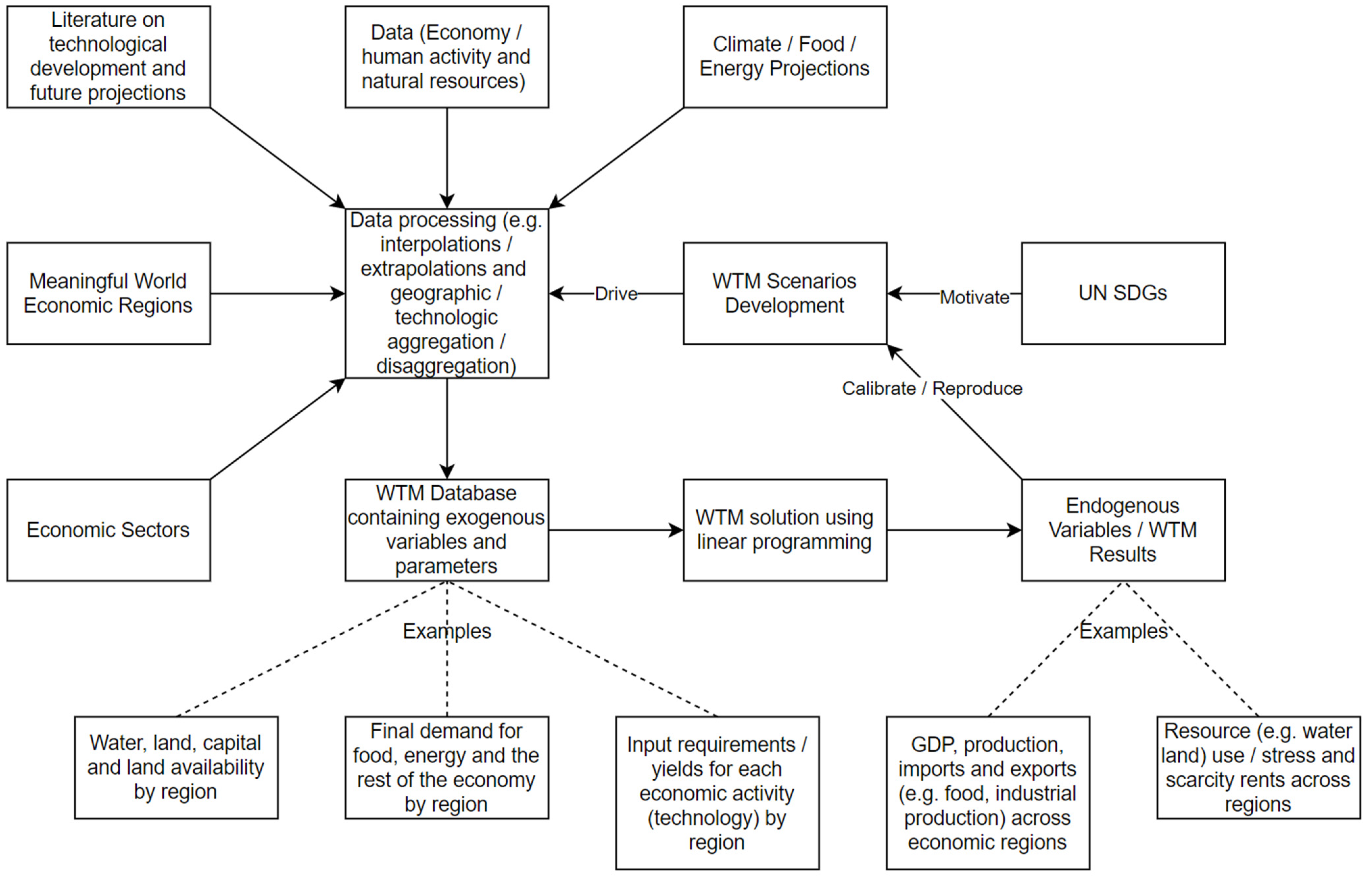
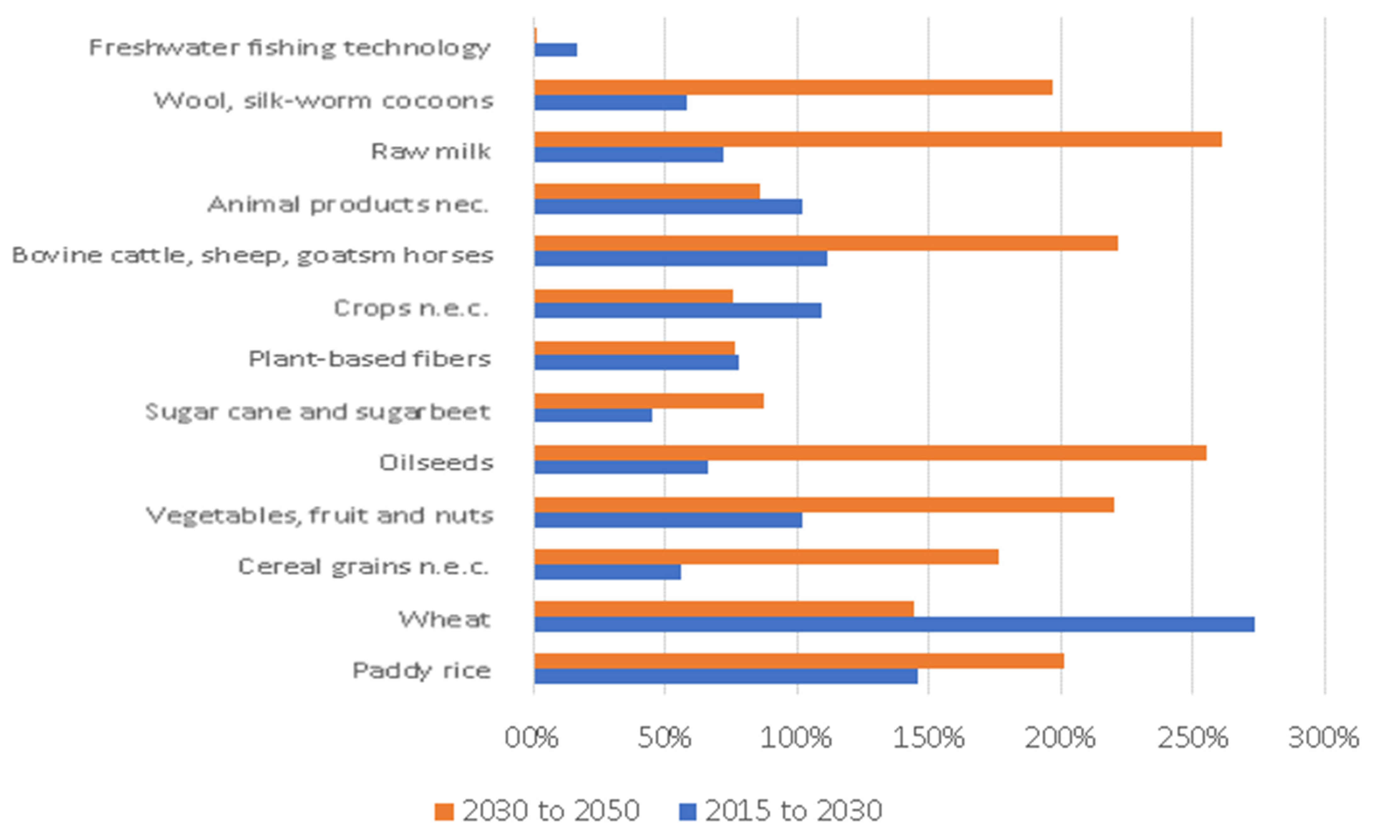
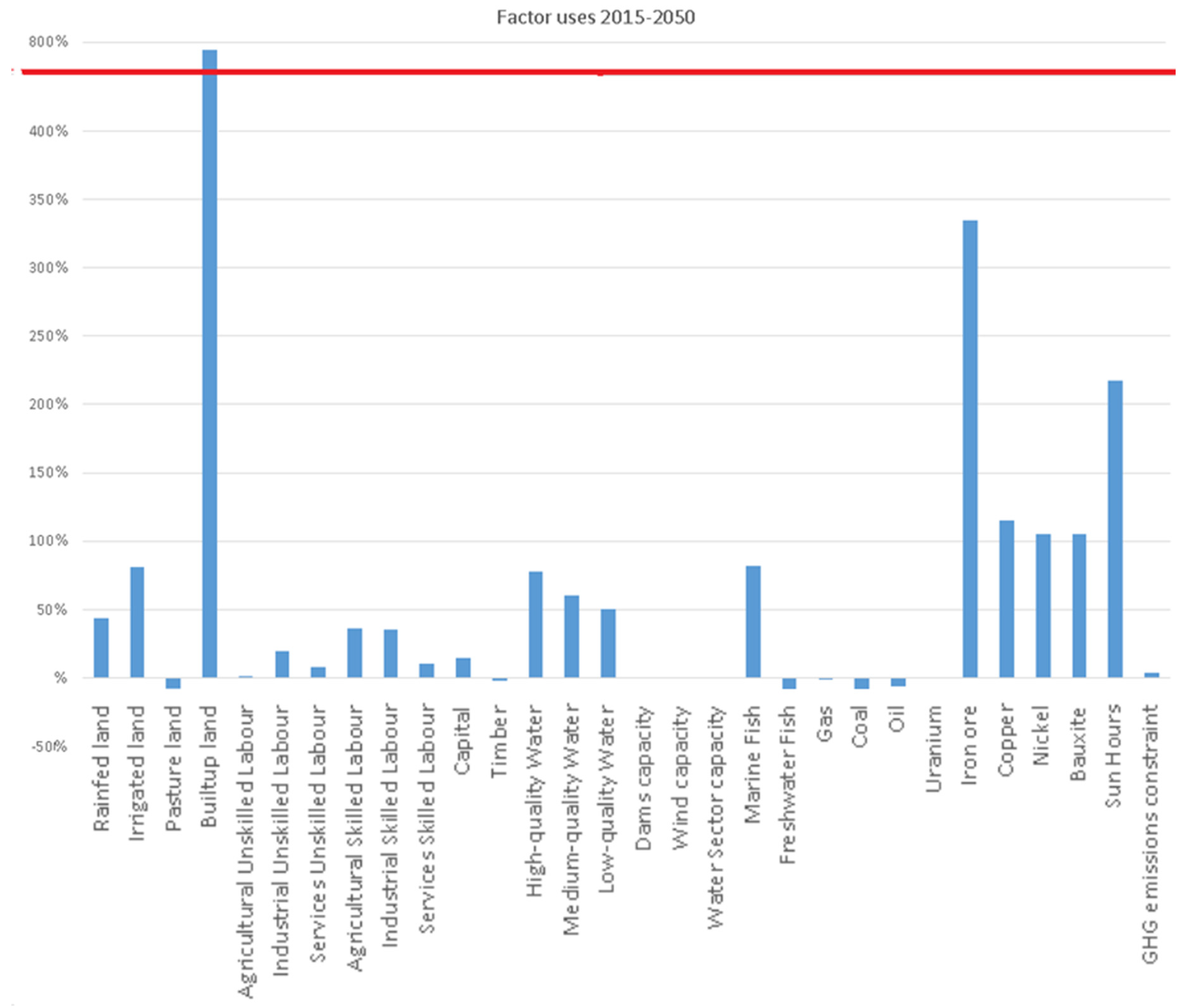
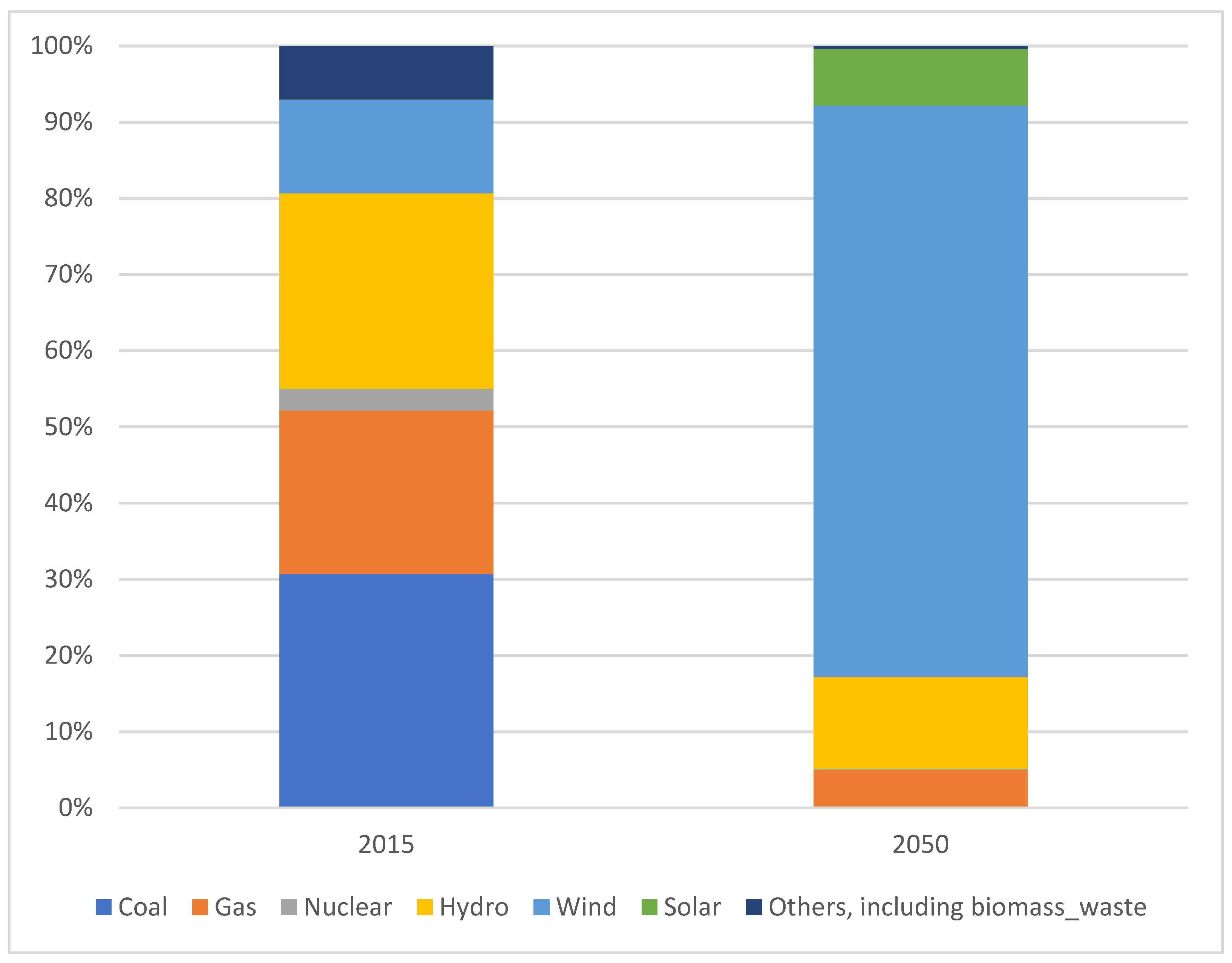
Table 1.
Sources for scenarios and how key factors change in each of them.
| SSP1 Sustainability | SSP2 Middle of the Road | SSP3 Inequality | SSP4 Regional Rivalry | SSP5 Fossil Fueled Development | |
|---|---|---|---|---|---|
| Population | SSP1 | SSP2 | SSP3 | SSP4 | SSP5 |
| Consumption data and GDP | SSP1 | SSP2 | SSP3 | SSP4 | SSP5 |
| Landcover | SSP1 | SSP2 | SSP3 | SSP4 | SSP5 |
| Food demand | SSP1 readapted with food products details (based on [83] | SSP2 from [83] | SSP3 from [83] | Based on SSP3 from [83] | Based on Average of scenarios 3 to 6 on RCP 8.5 [83] |
| Energy demand | Based on Final Energy SSP1 ([84], EIA [85]) | Based on Final Energy SSP2 ([84], EIA [85]) | Based on Final Energy SSP3 ([84], EIA [85]) | Based on Final Energy SSP4 ([84], EIA [85]) | Based on Final Energy SSP5 ([84], EIA [85]) |
| Water endowments | Water Baseline ↓ (increased environmental flows) | Water Baseline (based on Jackson et al. 2001 and FAO [86]) | Water Baseline | Water Baseline | Water Baseline |
| on ease of trade | Baseline | Baseline | Baseline ↑ | Baseline ↑↑ | Baseline |
| Technological changes (Reduction in materials intensity, in A and F) | Energy technologies based on [61,62,63,66,84,87]; agricultural technologies based on [46,88]; General technological changes based on [45,85,89] | ||||
| Emissions threshold | Paris Agreement and NDCs (for 1.5°) thresholds | Harmonized SSP data (2.6°–3.4° average in the main results presented) threshold | Harmonized SSP data (4.5° average in the main results presented) threshold | Harmonized SSP data (3.4°–4.5° average in the main results presented) threshold | Harmonized SSP data (3.4° average in the main results presented) threshold |
Note: All cells just indicating SSP scenarios are the SSP data taken from IIASA (see e.g., [34,35,82]). Available online: https://tntcat.iiasa.ac.at/SspDb/dsd?Action=htmlpage&page=40 (last accessed on August 2021). If several options exist, the Marker Scenarios (see SSP documentation of IIASA) are taken.
Table 2.
Summary of results by each scenario, in terms of FEW.
| FEW and Other Resources | By 2030 | By 2050 | ||||||
|---|---|---|---|---|---|---|---|---|
| SSP1 Sustainability | SSP2 Middle of the Road | SSP3 Inequality | SSP5 Fossil Fueled Development | SSP1 Sustainability | SSP2 Middle of the Road | SSP3 Inequality | SSP5 Fossil-Fueled Development | |
| Food demand and production | According to Valin et al. (2014) the food demand does not change much across SSPs, but this one is in line with less direct and indirect resources consumption | Current consumption patterns are more or less followed. Crop production reaches 2.7 billion tons. | Production of “wheat” (followed by rice) notably increases in the world, in several regions, not only in the baseline places such as EU, USA, India or Canada, but also expanded to Middle East and North Africa, Russia and Other Eastern Europe and West Asia. | Consumption patterns get closer to the developed countries ones. Meat and fish consumption are in general increased in developing countries. | Beyond 2030 demand growth for most crops and meat is projected to slow considerably. Protein content cannot exceed 40% under equitable diets. Billen et al. (2015) | According to Valin et al. (2014) the food demand does not change much across SSPs. Production of “vegetables, fruit and nuts” notably increases in India and China [83]. | According to Valin et al. (2014) the food demand does not change much across SSPs. Increased self-sufficiency at higher costs [83]. | According to Valin et al. (2014) the food demand does not change much across SSPs. Impacts of climate change on food production [83]. |
| Energy | Electrification is rapid, particularly in developing countries. Transformation towards public transport and electric or hydrogen cars. Low transport energy demand easing the mitigation challenge. | Demand for energy grows by 40% by 2030. Moderate modernization of final energy use. The picture is mixed when looking at traditional and modern energy carriers. | Slow growth, convergence and modernization in the global final energy mix. The electrification in developing regions is slow, with relative stagnant technologies. | Rapid electrification, particularly in developing countries. More conventional transport system with high demand for transp. services (decarbonization challenge). | Electrification is completed. Demand growth slows in China and India beyond 2030, slowing down global demand growth. | The use of liquids increases by 2/3 up to 2050 and remains roughly constant thereafter. Electricity consumption x2 from 2010 to 2050. The direct use of coal x2 by 2050 to fuel industrial development in Asia, Middle East and Africa. | Demand growth slows in China and India beyond 2030, slowing down global demand growth. | Electrification of most economies is completed. The energy transition is completed, but all the economy has high volumes of activity, with high requirements. |
| Water | There are no global total (high, medium and low) water challenges. | Moderate increases in water uses. | Agriculture is progressively homemade, affecting water scarcity, and showing other pressures, such as in the short run from the increase in wheat production. | Significant production takes place in regions which are relatively water scarce (China, India, South Asia, and Oceania). | There are no global total (high, medium and low) water challenges, but there is regional scarcity in medium and high-quality water type. Significant shifts to more water efficient technologies. | If in SSP1 a decrease of industrial water withdrawal is projected, here there is also some stabilization, but some increase for agriculture. | Increased self-sufficiency ⇒ localized environmental stresses. Agriculture (e.g., cereal production) challenged in India, China, the EU, affecting water scarcity (and other pressures). | After previous increases in water uses, up to 2050 these are stabilized. |
| Metals and Minerals in general | Demand for major metals grows between 30–50%, rare earth demand doubles from 2015 levels. | The extraction and use of primary (raw) materials is much more polluting than secondary (recycled) materials. | Compared to 2015 levels, demand for steel grows by 80%, copper by 70%. Aluminium, nickel, and zinc demand more than double. Many countries cannot access some minerals and (at a minimum) pay a higher price. | Recurrent supply bottlenecks for specialty metals as new technologies are widely deployed. Also, massive extraction has a wide range of polluting consequences, including toxic effects on humans and ecosystems. | While resources demand does not grow that much in other factors for SSP1 than others, in the case of minerals, some of them (related to batteries and energy transition) are highly demanded. | Construction and other industries materials demand grows in many places, e.g., China, implying high demand. | Demand growth for steel slows as the current infrastructure and construction boom in large emerging economies slowly goes down. | Demand is very high, with high scarcity rents obtained for some minerals. |
| Land | No major land pressures. | Harvested irrigated land is projected to expand around 6%. Pastureland use increases by 7% in 2050. | Cropland and pastureland pressures are localized in a few areas of the world, from both developing and developed countries (e.g., Japan and South Korea). Other natural habitats are reduced. | Land pressures are localized in a few areas of the world, especially in Africa and central/south America. Pastureland is reduced in the USA. | No major land pressures, although interestingly some increases from solar and especially biomass are relevant. | Harvested irrigated land is projected to expand around 15% (pastureland by 20%), mostly in developing countries (by regions: 17SS_Africa, 12SOAmerica, 11CS_America and 8India). | Land pressures are localized in many areas of the world, from both developing and developed countries, including the EU. | Land pressures localized in many areas of the world, especially in Africa and America. Harvested irrigated land rises up to 25%. |
| GHG | This scenario is the one where the emissions are constrained to keep the levels below 1.5 °C a t the end of the century. Annual 13–16 Gt CO2 equiv. | Around 30 annual Gt CO2 equivalent. | This scenario is the worse in terms of GHG emissions (40 Gt CO2 eq.). Countries do not benefit from best technologies and trade, and the narrative of regional rivalry makes difficult international agreements. | Fast growth leads to very high GHG emissions which do not deviate from surpassing the 2 °C target at the end of the century despite the technology improvements and Δ energy. | This scenario is the one where the emissions are constrained to keep the levels below 1.5 °C a t the end of the century. | Medium GHG emissions, which are inevitably driven up by population and affluence growth but buffered by technology improvements. | Very high GHG emissions which do not accomplish current climate targets, especially with some countries still with brown energy. | GHG emissions rise to ~50 yearly Gt CO2 equiv. by 2050. |
Source: own elaboration. Specifically, the variant of SSP1 provides the least of the increases, with only 10% more of land and water up to 2050. Still, its feasibility is only possible under a combination of reduced demand (as projected in the scenarios), a faster energy transition, and important technological advances that reduce the requirements of inputs per unit of production. (Without fast technical change and GHG emissions constraints, it is not possible to achieve the 1.5 °C target by the end of the century).
Publisher’s Note: MDPI stays neutral with regard to jurisdictional claims in published maps and institutional affiliations. |
© 2021 by the authors. Licensee MDPI, Basel, Switzerland. This article is an open access article distributed under the terms and conditions of the Creative Commons Attribution (CC BY) license (https://creativecommons.org/licenses/by/4.0/).
Share and Cite
MDPI and ACS Style
Cazcarro, I.; Dilekli, N. Developing the Food, Water, and Energy Nexus for Food and Energy Scenarios with the World Trade Model. Water 2021, 13, 2354. https://doi.org/10.3390/w13172354
AMA Style
Cazcarro I, Dilekli N. Developing the Food, Water, and Energy Nexus for Food and Energy Scenarios with the World Trade Model. Water. 2021; 13(17):2354. https://doi.org/10.3390/w13172354
Chicago/Turabian StyleCazcarro, Ignacio, and Naci Dilekli. 2021. "Developing the Food, Water, and Energy Nexus for Food and Energy Scenarios with the World Trade Model" Water 13, no. 17: 2354. https://doi.org/10.3390/w13172354
Note that from the first issue of 2016, this journal uses article numbers instead of page numbers. See further details here.