
Forecasting of Debris Flow Using Machine Learning-Based Adjusted Rainfall Information and RAMMS Model


1
Department of Urban and Environmental and Disaster Management, Graduate School of Disaster Prevention, Kangwon National University, Samcheok-si 25913, Korea
2
New Business Development Team, ECOBRAIN Co. Ltd., Jeju 63309, Korea
*
Author to whom correspondence should be addressed.
Water 2021, 13(17), 2360; https://doi.org/10.3390/w13172360
Submission received: 22 June 2021
/
Revised: 6 August 2021
/
Accepted: 22 August 2021
/
Published: 27 August 2021
(This article belongs to the Special Issue Debris Flows Research: Hazard and Risk Assessments)
Abstract
:In recent years, climate change and extreme weather conditions have caused natural disasters of various sizes and forms across the world. The increase in the resulting flood damage and secondary damage has also inflicted massive social and economic harm. Korea is no exception, where debris flows created by typhoons and localized heavy rainfalls have caused human injuries and property damage in the Wumyeonsan Mountain in Seoul, Majeoksan Mountain in Chuncheon, Sinnam in Samcheok, Gokseong in Jeollanam-do, and Anseong in Gyeonggi-do. Disaster damage needs to be minimized by preparing for typhoons and heavy rainfalls that cause debris flow. To that end, we need accurate prediction of rainfall and flooding through simulations based on debris flow models. Most of the previous literature analyzed debris flows using rainfall events in the past before debris flow occurrence, rather than analyzing and predicting based on rainfall predictions. The main body of this study assesses the applicability of hydrological quantitative precipitation forecast (HQPF) generated through a machine learning method named the Random Forest (RF) method to debris flow analysis models. To that end, this study uses scatter plots to compare and analyze the precipitation observation data collected from the areas hit by debris flows in the past, and the quantitative precipitation forecast (QPF) and HQPF data from the Korea Meteorological Administration (KMA). Based on the verified HQPF data, runoff was calculated using the spatial runoff assessment tool (S-RAT) model, and the soil amount was calculated to simulate the debris flow damage with a two-dimensional rapid mass movements (RAMMS) model. The debris flow simulation based on the said data indicated varying degrees of flow depth, impact force, speed, and damage area depending on the precipitation. The correction of the HQPF was verified by measuring and comparing the spatial location accuracy by analyzing the Lee Sallee shape index (LSSI) of the damage areas. The findings confirm the correction of the HQPF based on machine learning and indicate its applicability to debris flow models.
1. Introduction
In recent years, Korea has seen a rapid increase in the frequency and strength of heavy rainfall on account of changes in weather and environment brought on by climate change. These changes have inflicted growing social and economic damage on the country. Korea’s average annual precipitation is higher than 1200 mm, which is 1.6 times higher than the global average of 800 mm. The water intake rate is higher than 30%, which is one of the highest rates among the OECD countries [1]. Most of the precipitation is concentrated around the monsoon season in summer, which has been the cause of frequent typhoon and heavy rainfall damages. More than 65% of the Korean territory is covered in mountains. In the case of heavy rainfall, the runoff speed rapidly increases and causes floods, landslides, and debris flows.
According to the Landslide Information System of the Korea Meteorological Administration (KMA), global warming has increased the frequency of heavy rainfalls and the resulting damage by debris flows. The annual average damage area over the last decade is 226 ha, and the restoration efforts cost around KRW 43.6 billion.
Debris flow occurs when heavy rain falls on mountains and slopes, causing debris, trees, soil, stones, and rocks to flow into the valley creek, which flow down with massive force and inflict great damage on houses, farmlands, and roads [2].
As for debris flow cases in Korea, in July 2011, heavy rainfall in the central part of Korea took the lives of 43 people and damaged a total area of 824 ha near the Wumyeonsan Mountain in Seoul and the Majeoksan Mountain in Chuncheon. It was widely reported in Korea as it was the first case of debris flow hitting a mountainous area within a city downtown. In 2012, Typhoon Sanba damaged a total area of 491 ha and killed two people, and heavy rainfall in 2003 in Sancheong, Gyeongsangnam-do damaged a total area of 312 ha and killed three people. Heavy rainfall in 2017 damaged a total area of 94 ha and killed two people, Typhoon Mitag damaged a total area of 156 ha and three people in 2019, and heavy rainfall in 2020 damaged a total area of 93.25 ha and killed 16 people in Gokseong-gun, Anseoong-si, and other areas across Korea.
Cases in other countries include: Heavy rainfall in Venezuela in 1999 that claimed the lives of more than 20,000 and inflicted damage over KRW 180 billion; a landslide caused by heavy rainfall in Afghanistan in 2014, which killed around 2700 people, injured 14,000 people, and destroyed more than 300 houses; a series of heavy rainfalls, floods, and landslides in Sri Lanka that killed around 100 people and destroyed 140 houses in 2014, and killed around 280 people and damaged 4500 houses in 2017. As such, debris flows cause human injuries and deaths as well as property damages across the world. Causes of debris flow include the thawing of the soil in spring, uncontrolled logging and development, wildfire damaging the ecosystem, and many others. However, heavy rainfall remains the main cause of debris flow [3].
The following section reviews the latest research trends on debris flow in three areas: Simulation, precipitation forecast, and machine learning. First, [4] investigated the debris flow site in the Daeryongsan Mountain in Gagnwon-do in July 2013 and analyzed the behavioral characteristics of debris flows using the onsite data and the precipitation data. The authors used a digital elevation model (DEM) and stability index mapping (SINMAP) based on a digital map to compare the location of debris flows. The analysis showed that the high-risk areas and the actual sites are similar in slope-type debris flows. On the other hand, in valley-type debris flows, the debris flow sites matched the upper part of the valleys identified based on a topographic wetness index. Kim et al. selected flow parameters of the debris flows that hit the Wumyeonsan Mountain and used the FLO-2D model [5]. The representation accuracy for the damage area was assessed at 63% to 85%, which makes the FLO-2D model suitable for the analysis of the basin area damaged by debris flow. Jun et al. analyzed the risk levels of the areas damaged by debris flows using geographic information systems (GISs), statistical methods, and deterministic techniques [6]. The analysis found that the statistical methods are more relevant to the determination of debris flow risk areas than the SINMAP. As discussed above, there has been a constant flow of studies on damages caused by debris flows, and the characteristics of debris flows analyzed with GIS and modeling methods. However, few studies have been conducted to estimate and analyze the scale of debris flow damage. A study that uses data from actual debris flow sites and precipitation forecast data to analyze the scale of debris flow damage will be conducive to preventing future damage caused by debris flow.
Second, as for previous literature on precipitation forecast, [7] used the REGIONAL Data Assimilation Prediction System (RDAPS) data on the upstream area at the Soyanggang Dam from the KMA and a model used by the Korea Water Resource Corporation (KOWACO) to analyze dam inflow and accuracy. An analysis of the RDPAS accuracy confirmed the high accuracy of the quantitative and qualitative analysis of RDAPS and the average precipitation observed by automatic weather stations (AWS). The RDAPS-KOWACO model also produced highly accurate river runoff analysis results. Lee et al. proposed a short-term precipitation forecast method using the space distribution and an adjective model and applied it to Seoul [8]. Jung et al. used ground weather data measurements and a multi-layer neural network to propose a short-term precipitation forecast model, and the model was shown to offer better results than the existing models in terms of relevance and errors [9]. Kim et al. developed a short-term precipitation forecast model that considers non-linear correlations using the artificial neural network method, based on the wide-area automatic weather observation data from radiosondes and the predicted precipitations in the analyzed areas [10]. Verification using the Gamcheon Basin showed that the proposed model offers better results than predictions only based on ground weather data. Kim et al. sought to overcome the limitations of the existing linear extrapolation method incapable of simulating the growth and extinction of rainfalls by proposing a short-term precipitation forecast model based on radiowave speed and radar reflectivity using the reflectivity data of weather radars and multi-term regression equations [11]. Yoon et al. found that the simulation results of two-dimensional analyses of flooded areas using radar-predicted precipitation and ground-observed precipitation produced similar results [12]. The author concluded that flood damage could be prevented and reduced using prediction data with a similar level of accuracy to radar-predicted precipitation. Precipitation radars offer high space and time resolutions, which are useful for observing precipitation in mountainous areas, narrow areas, and steep slopes. The radar creates prediction data in the grid format, which makes the data highly useful for a distribution-type model. However, precipitation forecast using radars needs further research with regard to its uncertainty and quantification method. Along with studies on prediction using radars, more research seems to be needed on accurate and quantitative prediction using the fast-advancing machine learning methods, various models, and algorithms.
Third, machine learning is an area actively researched across various fields including video recognition, text recognition, stock price prediction, demand prediction, and others. In the field of meteorology, an increasing number of studies connect machine learning with flooding, famine, and other disasters. Kim et al. corrected ground precipitation data and radar precipitation data using an artificial neural network, and simulated runoff volumes by applying non-corrected radar precipitation data and corrected radar precipitation data to the quasi-distributive Modclark model, and compared the results with actual runoff data [13]. Jung et al. used the Okcheon station in the upstream part of the Daecheong Dam along the Geumgang River to study the observation data-based prediction of river level using deep learning algorithms [14]. The authors used TensorFlow and built long short-term memory (LSTM) and a multiple regression linear model to predict the water level in the target area. Choi et al. developed a prediction function for rainfall damage in the Seoul Capital Area (SCA) using machine learning methods (random forest, support vector machine, and decision making trees) [15]. The data on damage caused by rainfalls were defined as dependent variables, and the meteorological observation data were used as independent variables. The analysis showed that the support vector machine demonstrated the highest level of prediction power. Ham et al. developed a method to predict El Niños using the convolutional neural network (CNN), one of the deep learning technologies [16]. The training data were taken from the data from 1871–1873, which were used to verify the events between 1984 and 2017. The resulting accuracy was higher than 66.7%, and the author expected that the model would be applicable to El Niño predictions in the future. Fox et al. [17] predicted the hydrologic disturbance indexes using a Random Forest (RF) model at locations of fish communities in rivers [17]. Lee et al. used machine learning methods called Light GBM and XGBoost for hydrological precipitation correction, and analyzed five major rainfall cases between 2017 and 2018 in Seoul, Gangneung, and other areas [18]. The findings on the five rainfall cases clearly showed the correction effect of the two machine learning methods on the space distribution patterns of the rainfalls. Yen et al. used the echo state network (ESN) model and the DeepESN model to predict precipitation using rainfall, pressure, and humidity as parameters between 2004 and 2014 [19]. The study found that the correlation coefficients obtained with DeepESN produced superior results.
Disaster damage needs to be minimized by preparing for typhoons and heavy rainfalls that cause debris flow. To that end, we need accurate prediction of rainfalls and flooding. The KMA currently uses the ensemble prediction method to predict future precipitation. The ensemble prediction is designed to overcome the limitations of deterministic prediction based on single-figure forecasts, and predicts the future in probabilistic terms with diverse models with different initial conditions, physical processes, and boundary conditions [20]. The KMA provides rain forecasts in various formats including short-term, medium-term, and long-term forecasts, neighborhood-level forecasts, national forecasts, and special forecasts. Many researchers in Korea tackled the prediction method using radars and satellites that provide information on non-measured areas and evenly distributed data. However, as their use is limited by the lack of accuracy, radar and satellite data are used after correction based on accurate ground data.
This study analyzes runoffs and debris flows in areas actually hit by debris flows by producing hydrological quantitative precipitation forecast (HQPF) using a machine learning-based prediction model and assesses its applicability to damage scale analysis. This study also reviewed precipitation forecast methods and the relevant parameters, and designed an HQPF algorithm. As for the machine learning method, this study calculated precipitation forecasts using the Random Forest (RF) method, which creates multiple training data from a single dataset and creates multiple decision-making trees through multiple learning and combines them to improve prediction power. It also verified the calculated HQPF with statistical indexes and scatter plots. Based on the collected precipitation data and topological data, runoff volumes were calculated using the spatial runoff assessment tool (S-RAT) model, and a soil volume calculation equation was used to calculate possible soil volumes. The calculations were applied to a two-dimensional rapid mass movements (RAMMS) model to simulate the scale of debris flow damages. Then, this study conducted a Lee Sallee Shape Index (LSSI) analysis on the damage area results to verify the precipitation forecast accuracy and the model’s applicability. Figure 1 shows the research flow of this study.
2. Theoretical Background
2.1. Machinge Learning (Random Forest)
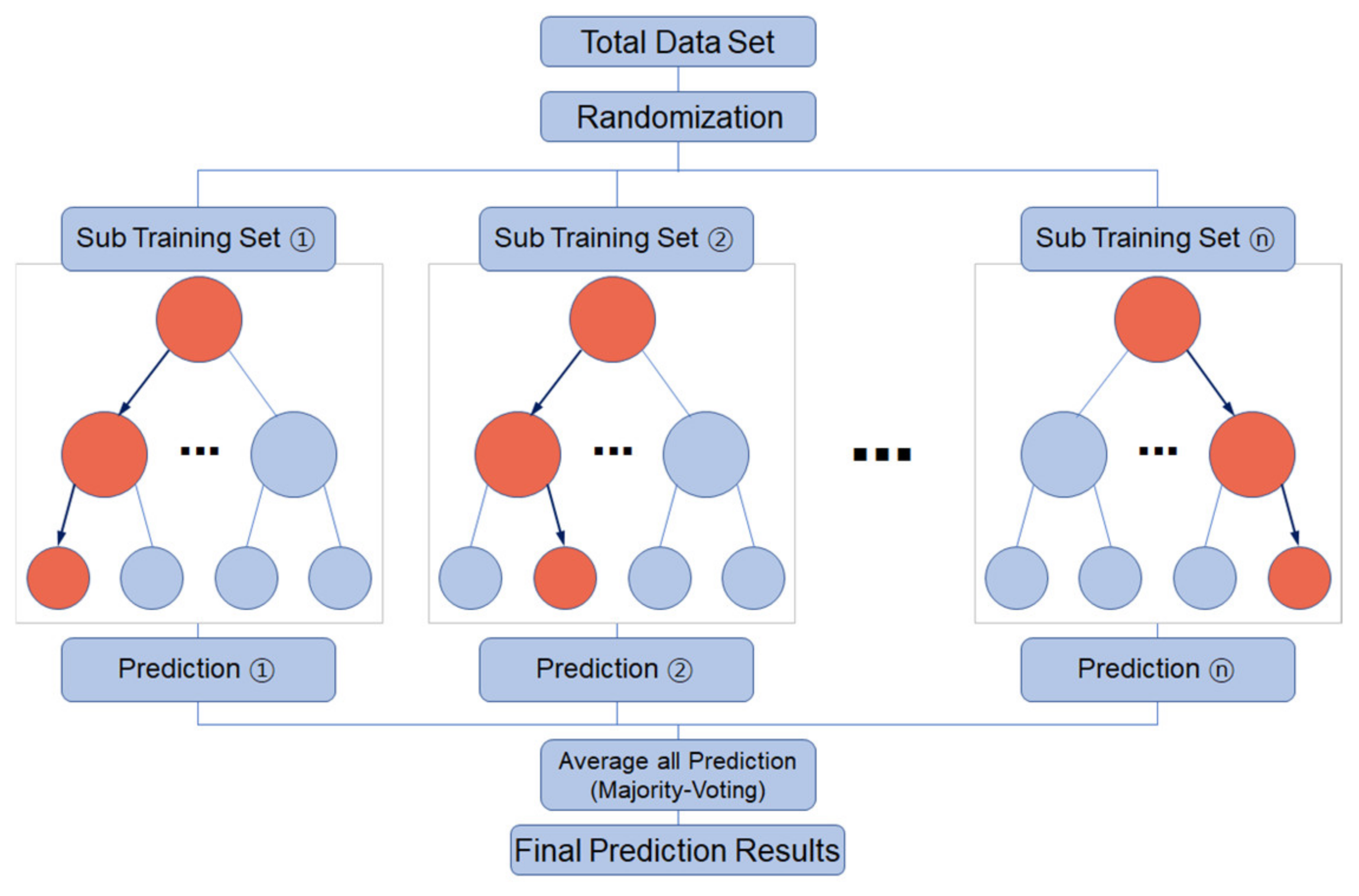
Machine learning is regarded as a sub-field of artificial intelligence (AI). In machine learning, a computer learns as a human would using programs and algorithms, and uses what it learns to develop technologies and make decisions. The RF method improves prediction power by creating a large number of decision-making trees [21]. The decision-making tree model makes predictions by creating and learning training data from one dataset. On the other hand, the RF model produces multiple training data from a single dataset, and creates multiple decision-making trees through multiple learning. The results from this learning are combined to improve prediction power [22]. In cases where the target variable is a continuous variable, and there are explanatory variables, variables are randomly selected from each division to create a tree [23]. The observations not used in the individual decision-making tree learning process are called out-of-bagging (OOB) observations, which are used to estimate prediction probabilities and confirming cause variables. The prediction probability of observations , for each observation belonging to Category (0 or 1) is defined as shown in Equation (1).
where is an indicator function 1 when the value in the parentheses is true, and 0 when the value is 0, and represents the forecast category. means the th decision-making tree. is the set of decision-making trees used to predict the category of observations in . In other words, it is the percentage of the number of decision-making trees predicted to be in , against the total number of decision-making trees used to predict [24]. Figure 2 shows the concept of random forest.
2.2. Spatial Runoff Assessment Tool (S-RAT)
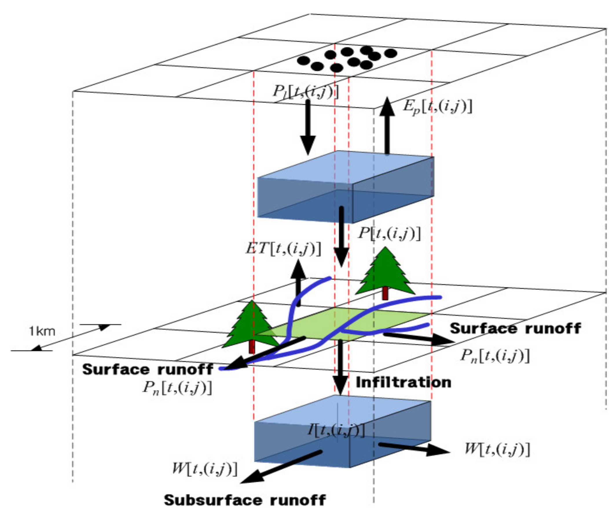
The S-RAT model is a distribution-type precipitation-runoff model designed to simulate temporal and spatial changes in runoff volumes in an area by dividing the target area into grids, and to calculate the conceptual water balance at an interval for each grid [13]. The S-RAT model calculates the infiltration and direct runoffs in each grid using the SCS curve number (CN) method. The CN data are generated and calculated by providing a soil map and a land use map.
where is potential water volume; is CN for each grid.
where is water content of the stormwater storage tank (); is capacity of the stormwater storage tank.
where is runoff beneath the surface, (mm) is direct runoff, and is a non-dimensional constant/conceptual parameter. Equation (7) represents a weight conservation control equation of the stormwater storage tank using Equations (2)–(6). Equation (7) can be analyzed using the fourth order Runge–Kutta method.
where E[t,(i,j)] is the effective evapotranspiration.
The applicability of the S-RAT model can be confirmed through paper [25].
Figure 3 shows a diagram of the grid type water balance calculation concept.
2.3. Debris Flow Simulation
Debris flow means debris, sand, pebbles, and other floating materials flowing down a slope on account of rainfall. Climate change and the resulting extreme weather events have increased the damage inflicted by debris flows, and a wide range of software has been developed and released to help simulate the occurrence, progress, and damage volume of debris flow.
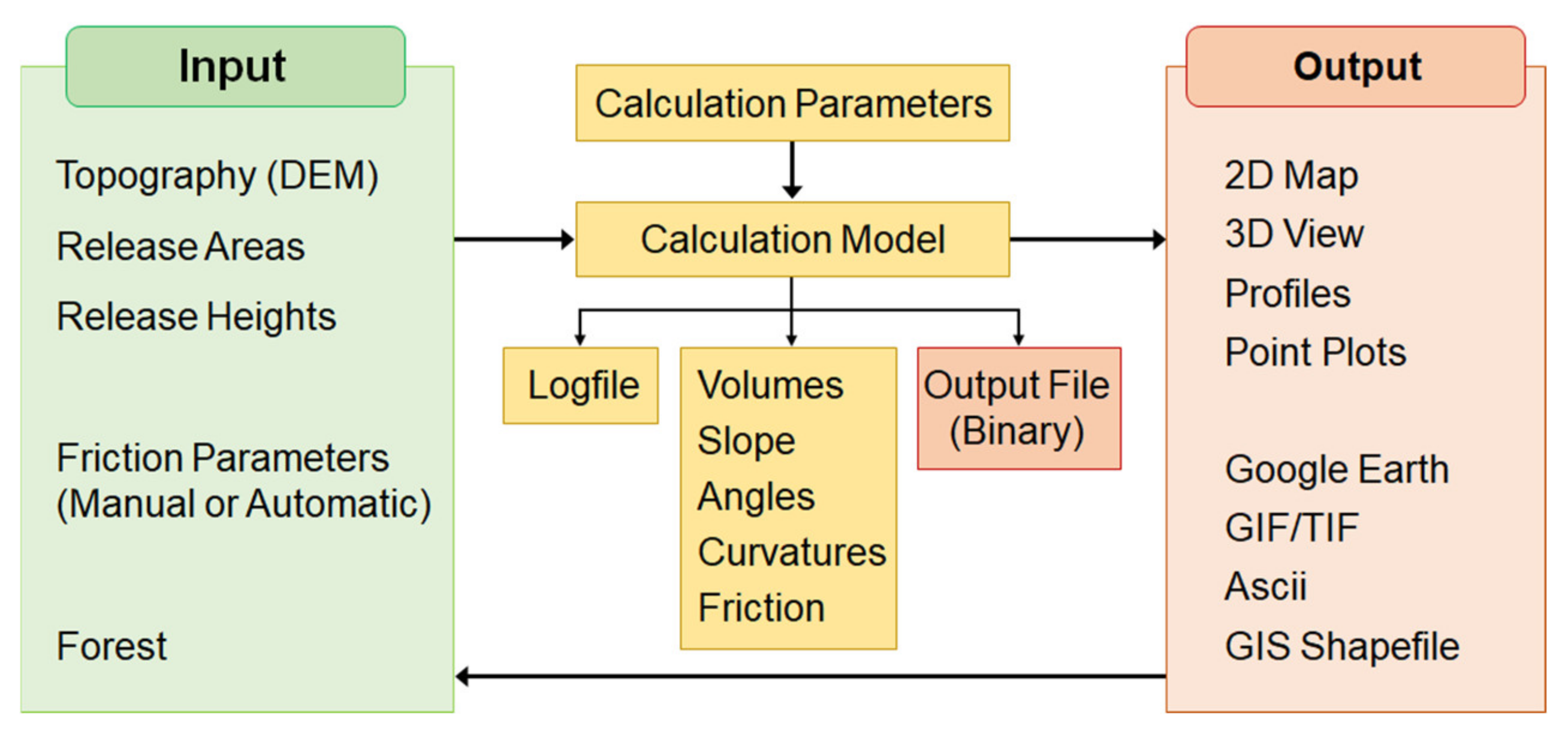
2.3.1. Two-Dimensional Rapid Mass Movements (RAMMS) Model
Unlike other models that only provide static data on debris flows, the RAMMS model is a dynamic model capable of providing dynamic analysis results over time. It offers analysis debris flows, rockfalls, or avalanches on a DEM. The basic equation of the model is based on the Vollemy–Salm method, and expressed as shown in Equation (8).
where is frictional force (), is cohesiveness to the floating materials, is viscosity coefficient, is gravitational acceleration (), is density (), is flow rate (), and is vertical stress (Mpa) against the active plane. is the flow material with cohesive force, and becomes 0 when = 0, and = 0. An increase in increases the friction force, which increases shearing stress and weakens the debris flow or avalanche [26]. RAMMS employs a Voellmy-fluid friction model(9). This model divides the frictional resistance into two parts: A dry-Coulomb type friction (coefficient μ) that scales with the normal stress and a velocity squared drag (coefficient ξ).
where is the flow density, gravitational acceleration, the slope angle, the flow height, and the flow velocity. This model has found wide application in the simulation of mass movements, especially snow avalanches. The Voellmy model has been in use in Switzerland for a long time and a set of calibrated parameters is available.
2.3.2. Calculation of Soil Volume
Debris flow simulation using the RAMMS model requires a number of input data including a DEM, peak runoffs, and soil volume. The density of debris flow has a great effect on soil volume and debris flow damage. Debris flow takes one of the following three forms depending on the river bed slope—stony debris flow, immature debris flow, and turbulent water flow—and the following formula is applied [28,29].
Stony debris flow occurs; .
Immature debris flow occurs; .
Turbulent water flow with bed load transport occurs; .
where is soil and sand density, is plastic density (), is water density (), is internal frictional angle (), is water surface slope (), is non-dimensional threshold shear stress, is non-dimensional shear strength.
The possible runoff soil volume at max precipitation was calculated using the equation proposed by the National Institute for Land Infrastructure Management [30].
where is possible soli runoff (), is 24-h cumulative precipitation (), A is basin area (), is prosity, is runoff correction rate.
3. Analysis and Results
3.1. Selection of Analysis Areas
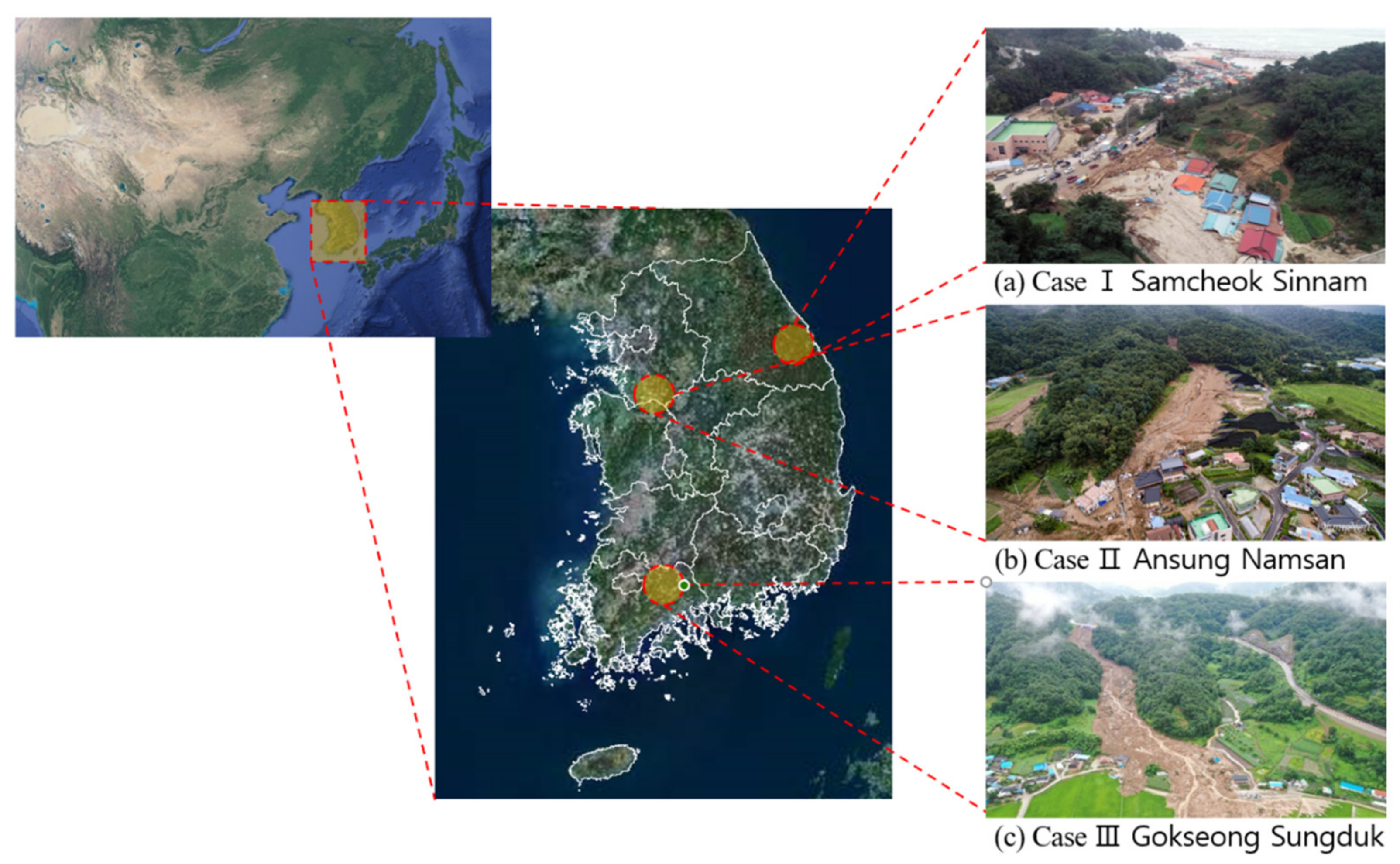
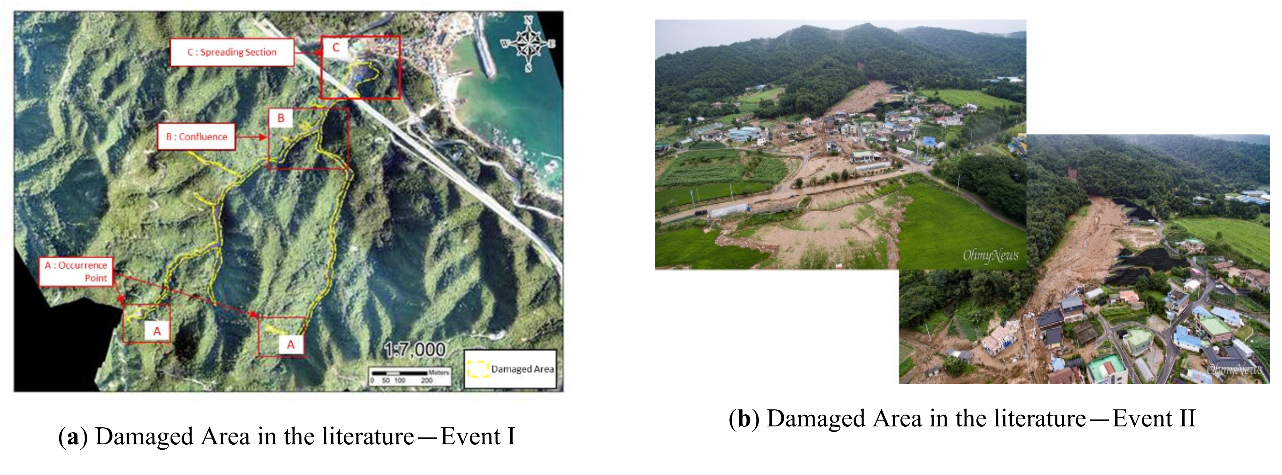
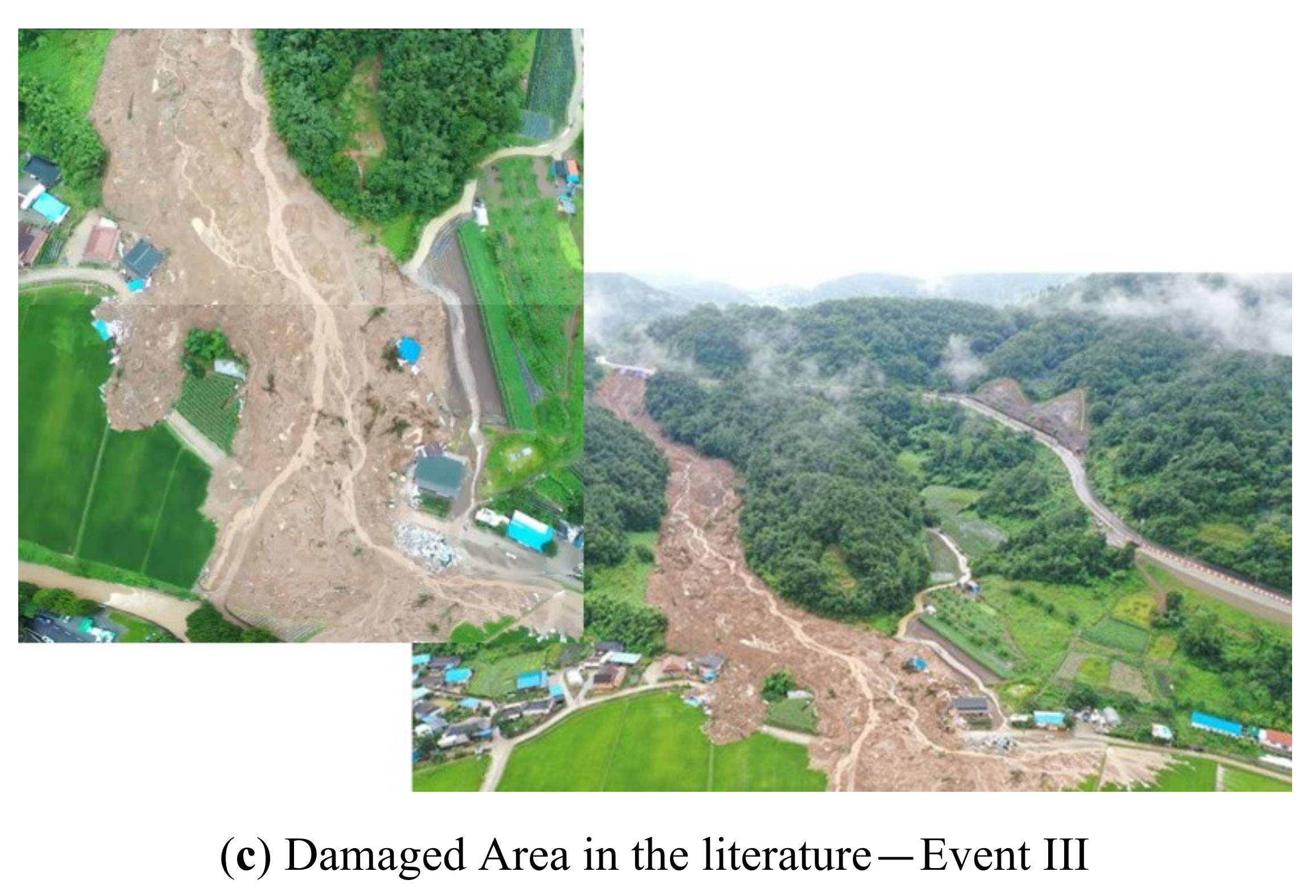
This study analyzed debris flow damage in areas damaged by debris flows in 2019 and 2020. The selected areas were Samcheok, Gangwon-do (October 2019, Event I), Anseong, Gyeonggi-do (August 2020, Event II), and Gokseong, Jeollanam-do (August 2020, Event III). In Event I, Sinnam Village in Samcheok was hit by heavy rainfall measuring 484 mm over 24 h, during which debris flow damaged 65 houses, destroyed 52 houses, and killed one person. In Event II, Namsan Village in Anseong was hit by heavy rainfall measuring 244 mm over 24 h, during which debris flow destroyed five houses and killed one person. In Event III, Seongdeok Village in Gokseong was hit by heavy rainfall measuring 494 mm over 24 h, during which debris flow destroyed five houses and killed five people. The locations and site photographs of Events I, II, and III are as shown in Figure 5.
3.2. Correction and Verification of Precipitation Forecast Using Machine Learning
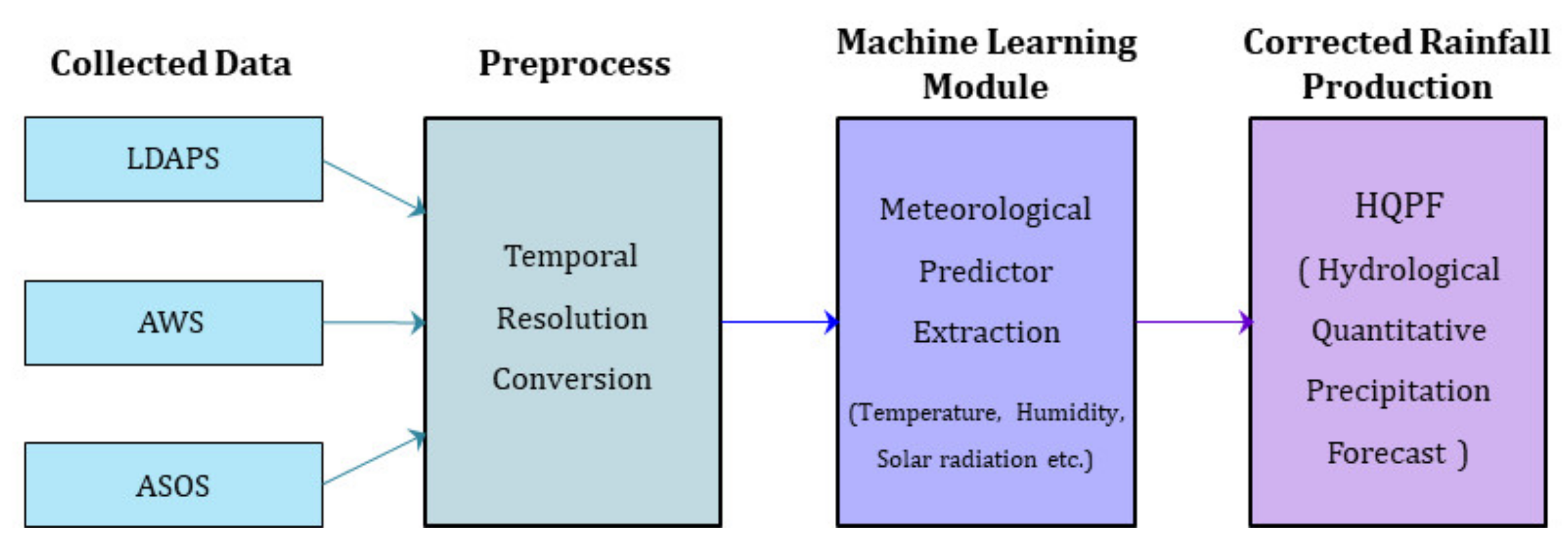
Rainfall is a non-linear event, which is not readily available for linear analysis. To overcome this limitation, this study used the RF machine learning method to improve precipitation forecast accuracy. The precipitation forecast correction mechanism was developed in three stages: Pre-processing (extracting forecast factors to be used as input data for machine learning); machine learning (using the input data for machine learning); and post-processing (generating precipitation forecast by correcting the precipitation produced through machine learning) [18]. The number of decision trees was set at 300, and the default values were used for the other parameters. The input data for machine learning included the AWS and automated surface observing system (ASOS) data from the KMA, and the forecast data extracted from the KMA’s Local Data Assimilation Prediction System (LDAPS) using the linear interpolation method. Figure 6 shows a schematic diagram of the machine learning process.
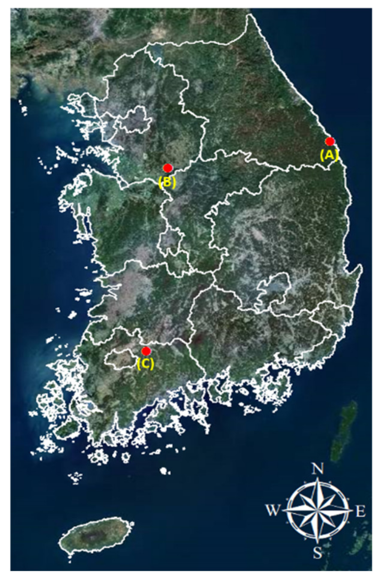
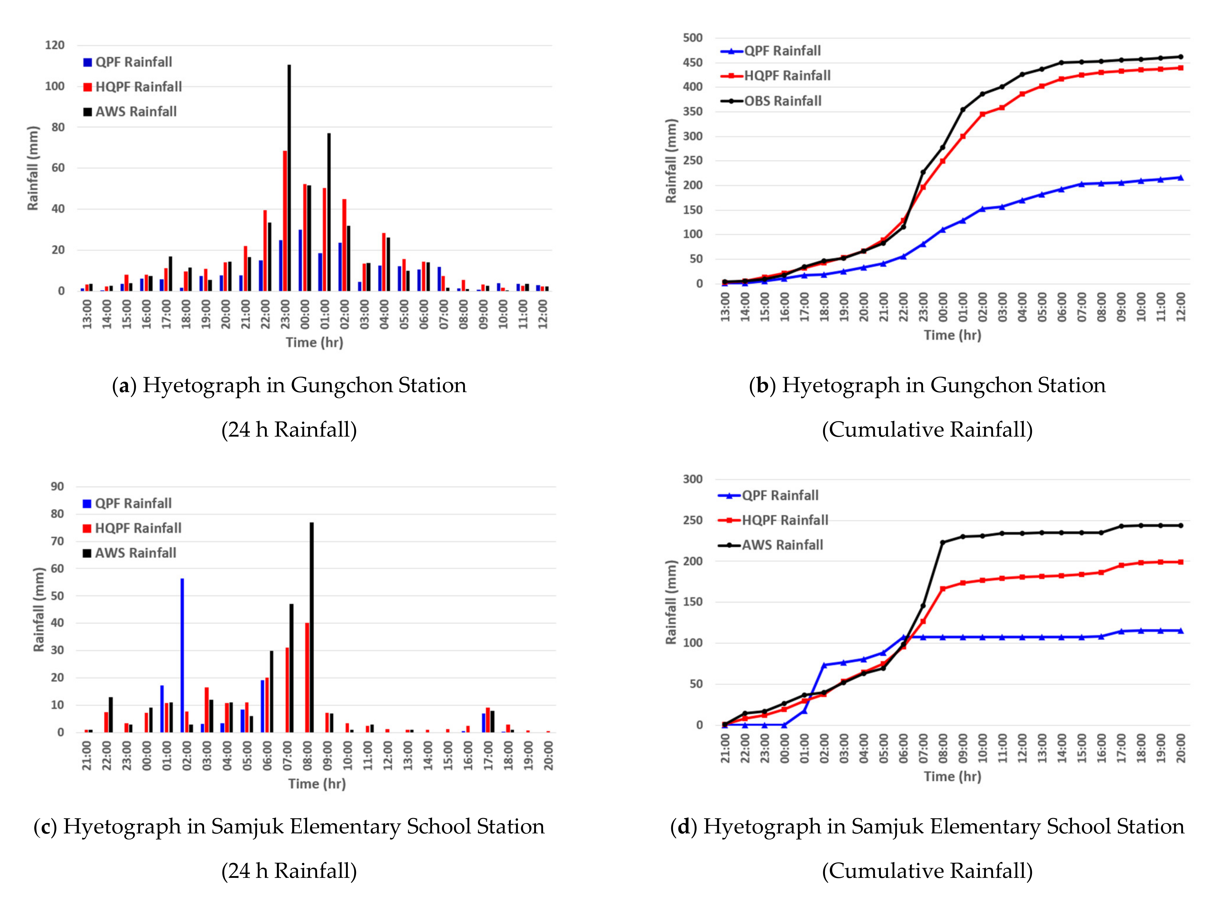
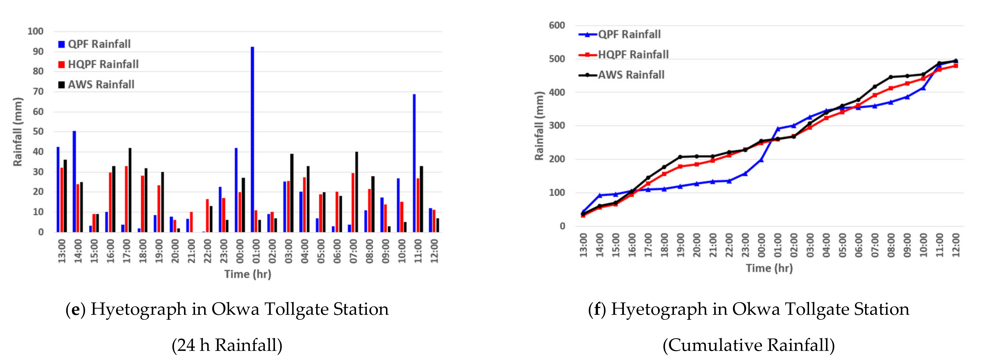
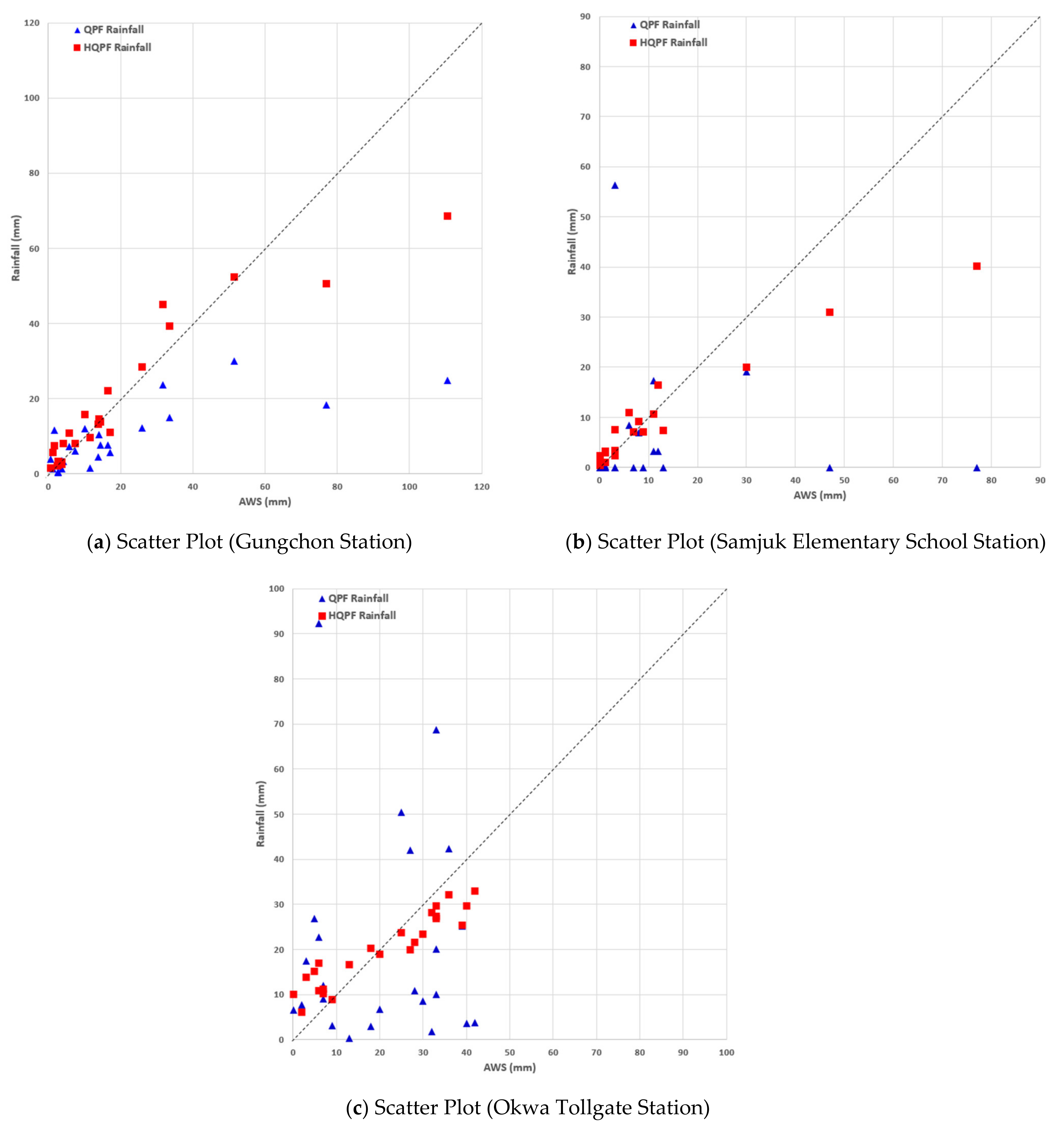
The precipitation observations used in this study consisted of the raw data from KMA AWS and the T/M observation stations at Flood Control Offices. The precipitation forecast data from the KMA were used for the QPF, and the precipitation data corrected and produced through the machine learning process were used for the HQPF. Then, before calculating precipitation forecasts for the debris flow damage areas, precipitation forecasts were calculated and verified for the AWS near the damage areas. The AWS were Gungchon for Event I, Samjuk Elementary School for Event II, and Okwa Toll Gate for Event III. The location of the station is listed in Figure 7, and the AWS data, QPF, and HQPF are listed in Figure 8.
The accuracy of the HQPF was verified using three indicators and a scatter plot. The three indicators were: Mean absolute error (MAE), normalized peak error (NPE), and peak timing error (PTE). A value of MAE or NPE closer to 0 means less errors, and a PTE value close to 0 indicates closeness to the peak precipitation time.
where is observed precipitation, is corrected precipitation, is the number of data, and are precipitation forecast and peak pre-forecast, respectively, and and is time when the corrected precipitation and peak precipitation forecast occurs.
Table 1 shows the three verification results for QPF and HQPF of Events I, II, and III. Across all events, HQPF show better correction results than QPF.
Figure 9 shows the scatter plot to identify the correlation between QPF and HQPF against the AWS precipitation data. The value of the determinant factor R2, which increases at low data disparity and decreases at high data disparity, was 0.6188 for QPF and 0.8733 for HQPF on the scatter plot of the Gunchon AWS in Event I. In Event II, the value was 0.0001 for QPF and 0.9278 for HQPF. In Event III, the value was 0.0004 for QPF and 0.883 for HQPF. The findings confirm that, across all events, HQPFs were corrected better than QPF.
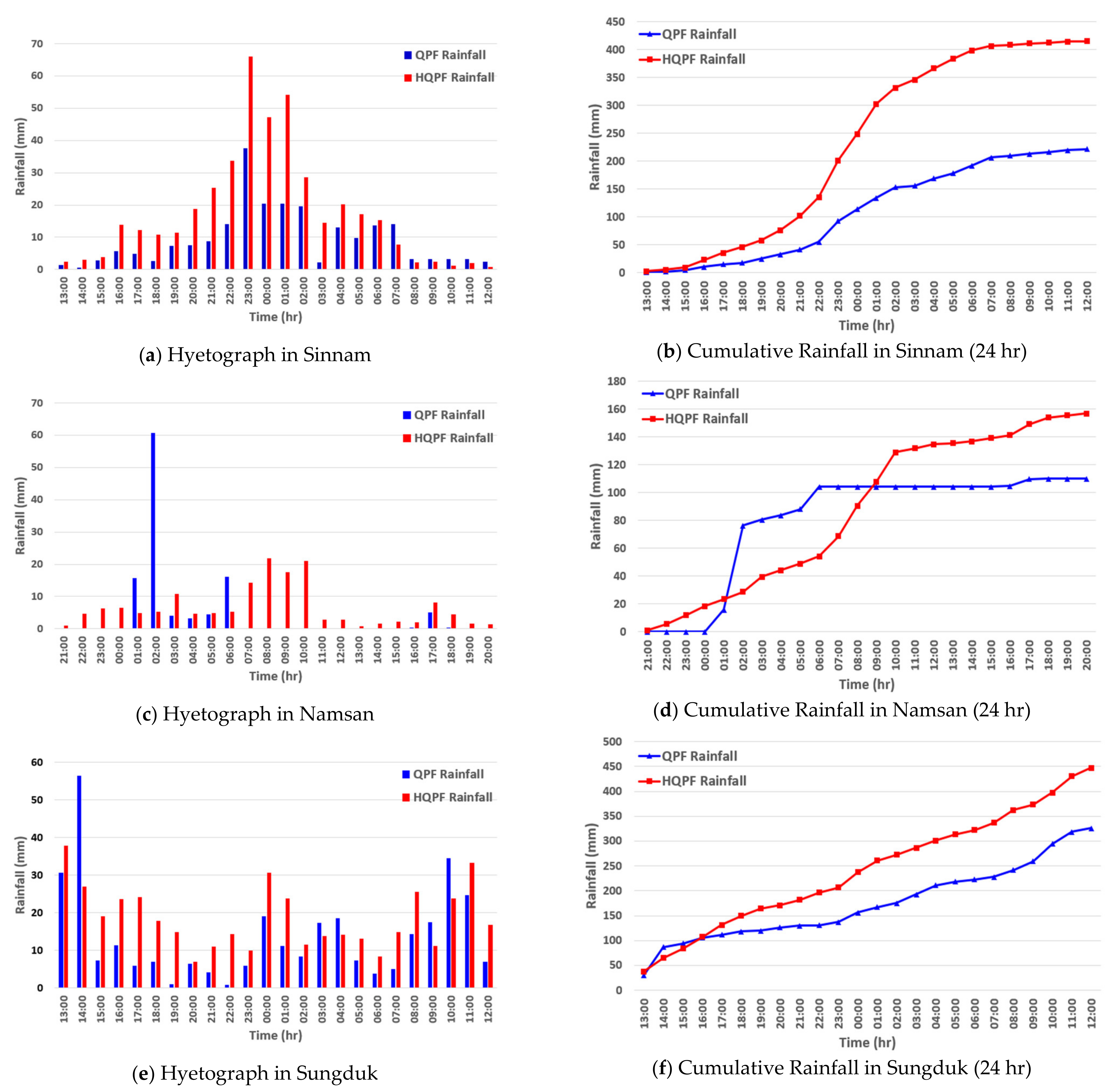
Based on the finding that the HQPFs were corrected better than the QPFs and closer to the AWS, this study simulated the runoff volumes and debris flows by calculating the QPF and HQPF of the actual damage areas. Figure 10 shows the 24-h cumulative precipitation and the precipitation map of the QPF and HQPF of the actual damage areas in Events I, II, and III.
3.3. Debris Flow Prediction Using Debris Flow Simulation
3.3.1. The Collection and Input Data Construction of Runoff Simulation
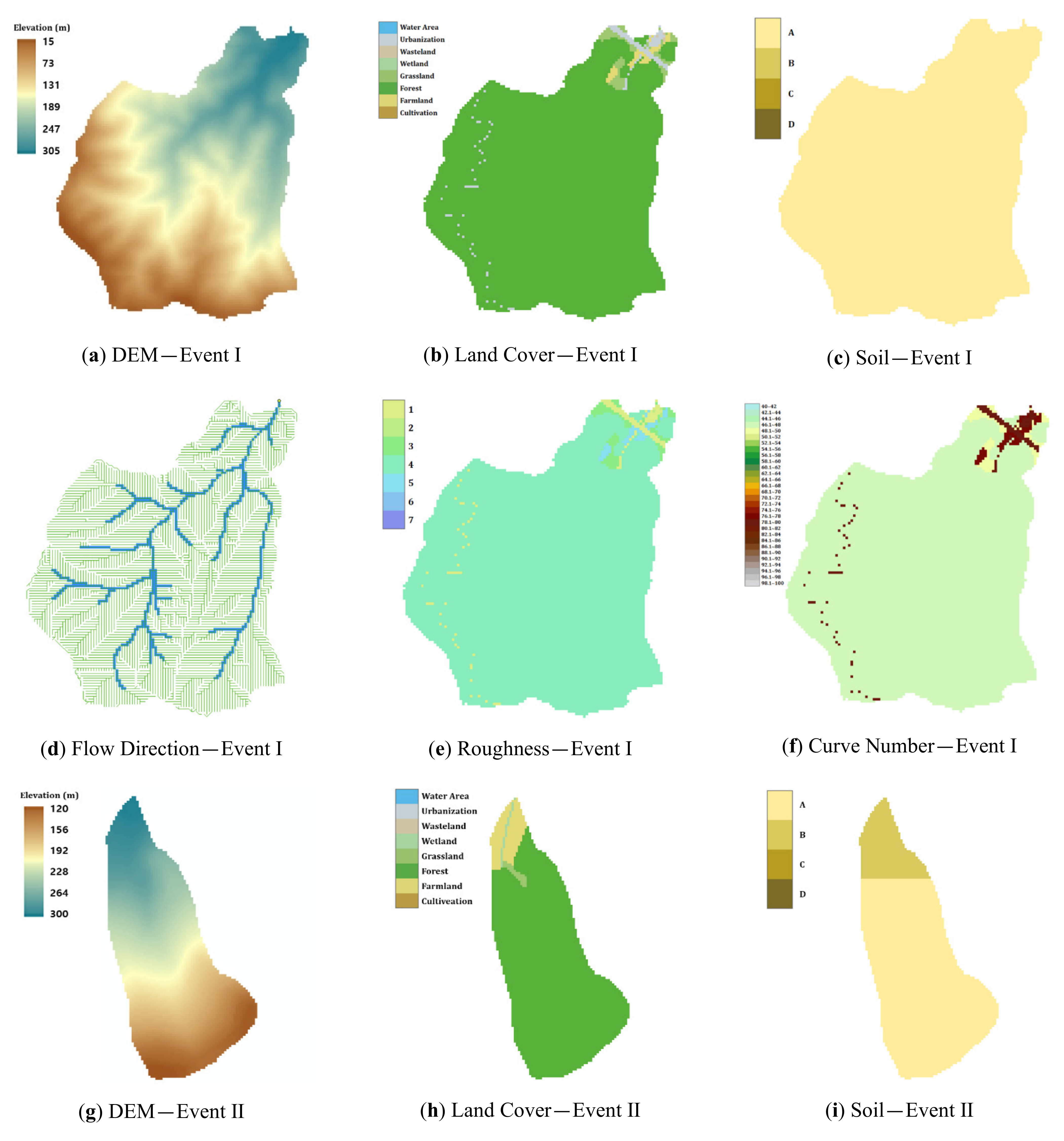
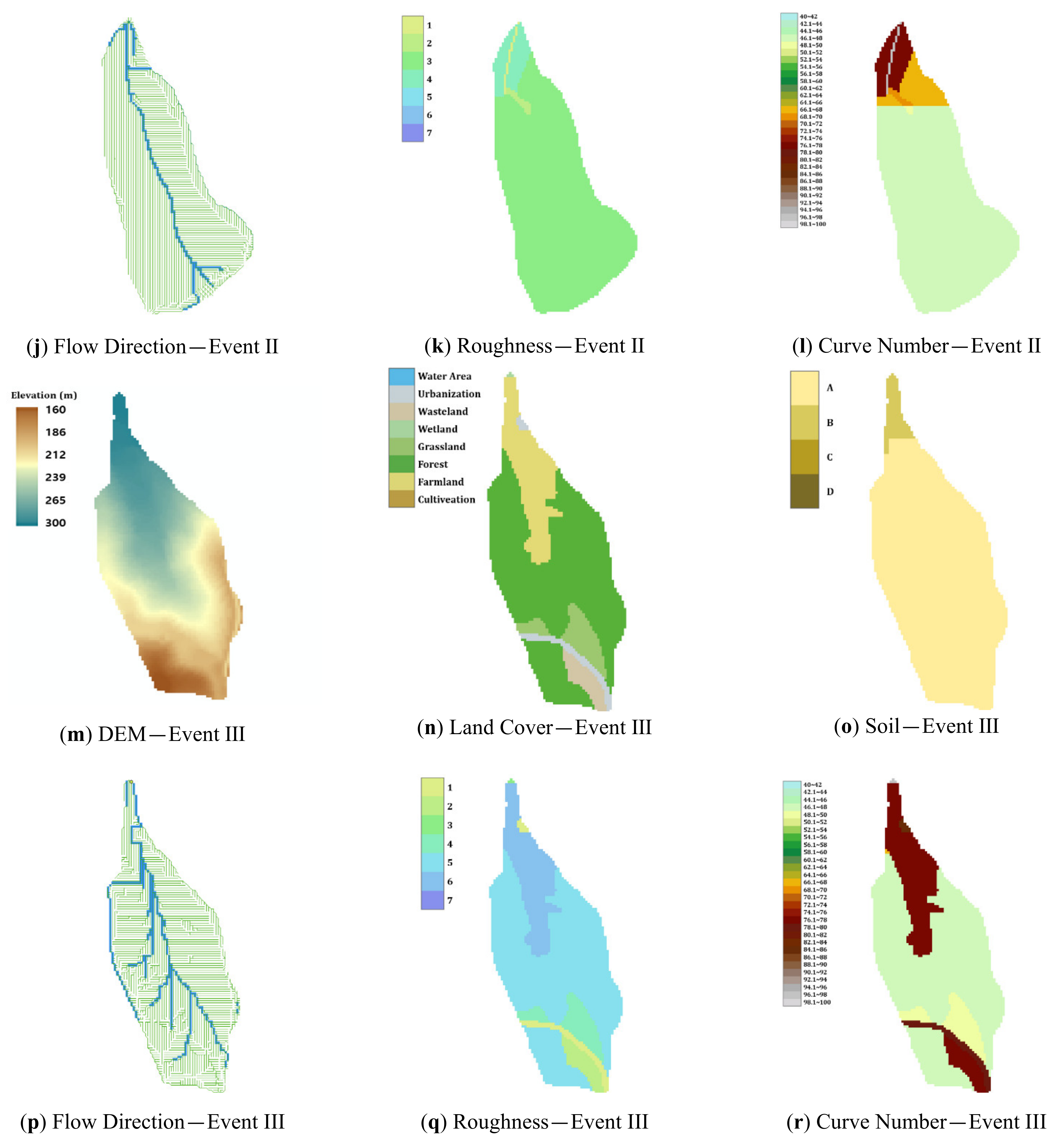
We used the basic topographical data using the precipitation data and the DEM, the land cover, and the soil map. Figure 11 shows the flow direction, roughness, and curve number data from the DEM, LC, soil map, and S-RAT model for Events I, II, and III. A to D in the soil group is classified according to infiltration rate and other properties (Type A—soils with high infiltration rates, even when thoroughly wetted and consisting chiefly of deep, well-drained to excessively drained sands or gravels; Type B—soils with moderate infiltration rates when thoroughly wetted and consisting chiefly of moderately fine to moderately coarse textures; Type C—soils with slow infiltration rates when thoroughly wetted and consisting chiefly of soils with a layer that impedes downward movement of water, or soils with moderately fine to fine textures; Type D—soils with very slow infiltration rates when thoroughly wetted and consisting chiefly of clay soils with a high swelling potential). 1 to 7 in the roughness group is the matrix of the Strickler roughness for the hillslope (). For the curve number group, the modified curve number method is used.
3.3.2. Runoff Volume Calculation (S-RAT)
We used the input data to simulate precipitation and runoff using the S-RAT model (Figure 12).
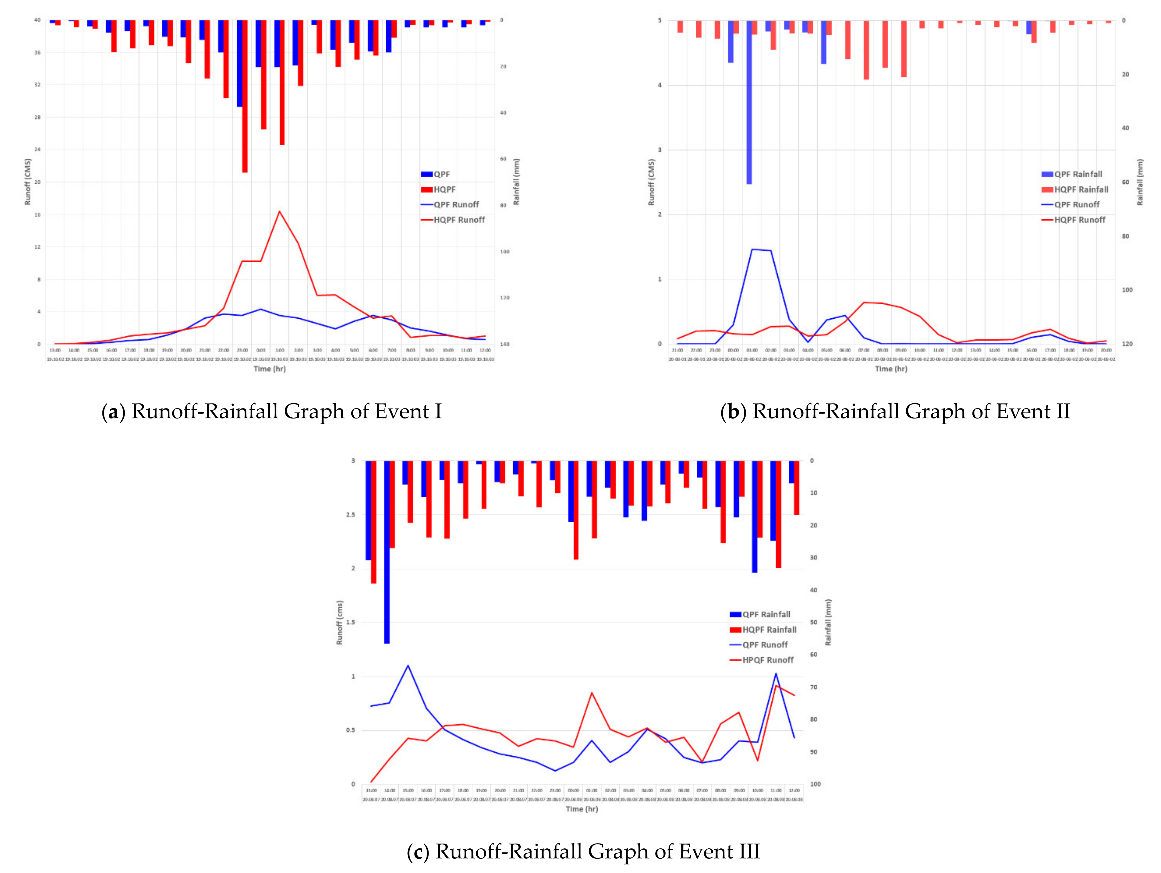
Using the QPF, the peak runoff of Event I (Sinnam Village, Samcheok) was 4.32 cm as of 3 October 2019, 00:00; the total runoff was 45.6 cm. For the HQPF, the peak runoff and the total runoff were simulated at 16.40 cm and 90.18 cm, respectively.
Using the QPF, the peak runoff of Event II (Namsan Village, Anseong) was 1.46 cm as of 2 August 2020, 01:00, the total runoff was 4.85 cm. For the HQPF, the peak runoff and the total runoff were simulated at 0.64 cm and 5.16 cm, respectively.
Using the QPF, the peak runoff of Event III (Seongdeok Village, Gokseong) was 1.1 cm as of 7 August 2020, 15:00, the total runoff was 10.4 cm. For the HQPF, the peak runoff and the total runoff were simulated at 0.92 cm and 11.25 cm, respectively.
3.3.3. Calculation of Soil Volume
This study calculated the soil volumes using the runoff volumes based on the runoff-rainfall analysis and the soil density calculated with the equation proposed by NILIM. The plasticity density (), water density (), internal frictional angle (), and average slope () were used to calculate the soil density (). The calculated , porosity (), basin area (), runoff correction rate (), and 24-h cumulative HQPF () were used to calculate each possible soil runoff volume () (Table 2).
In Event I, the soil density () was 0.32, the 24-h cumulative HQPF was 415 mm, and the possible soil runoff was 84,644 m3 for HQPF. In Event II, the soil density () was 0.42, the 24-h cumulative HQPF was 157 mm, and the possible soil runoff was 14,479 m3 for HQPF. In Event III, the soil density () was 0.28, the 24-h cumulative HQPF was 448 mm, and the possible soil runoff was 18,837 m3 for HQPF.
3.3.4. Debris Flow Simulation
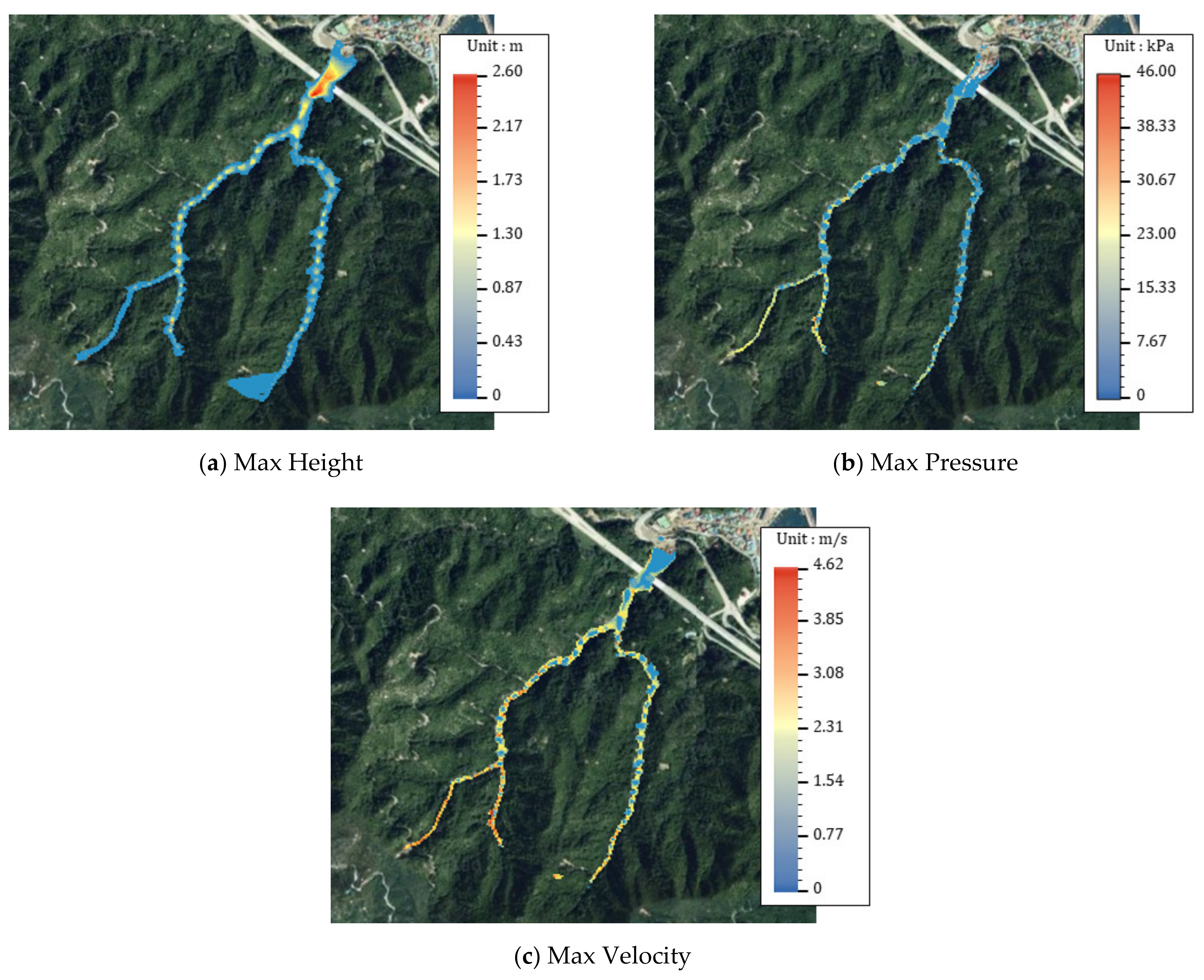
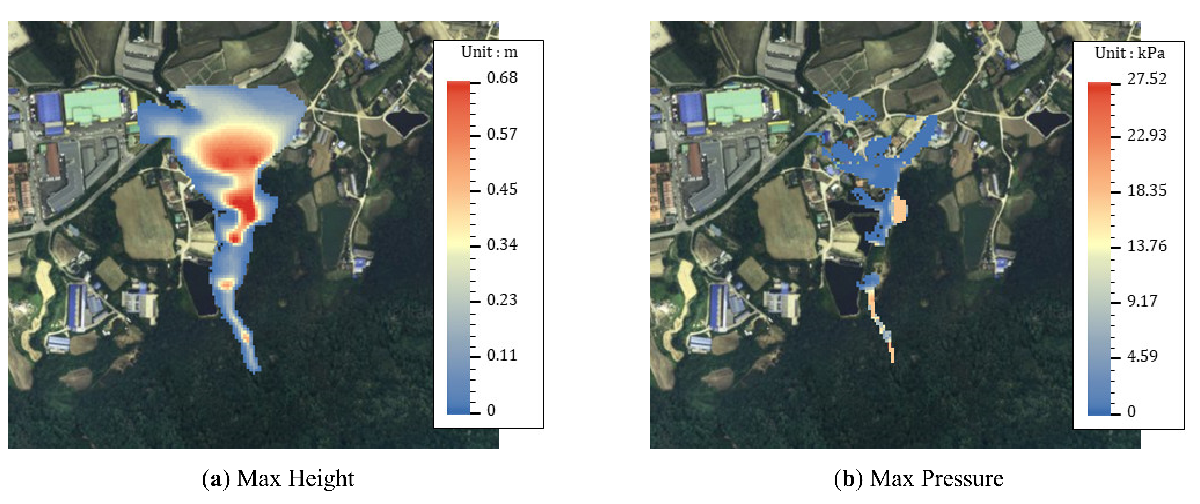
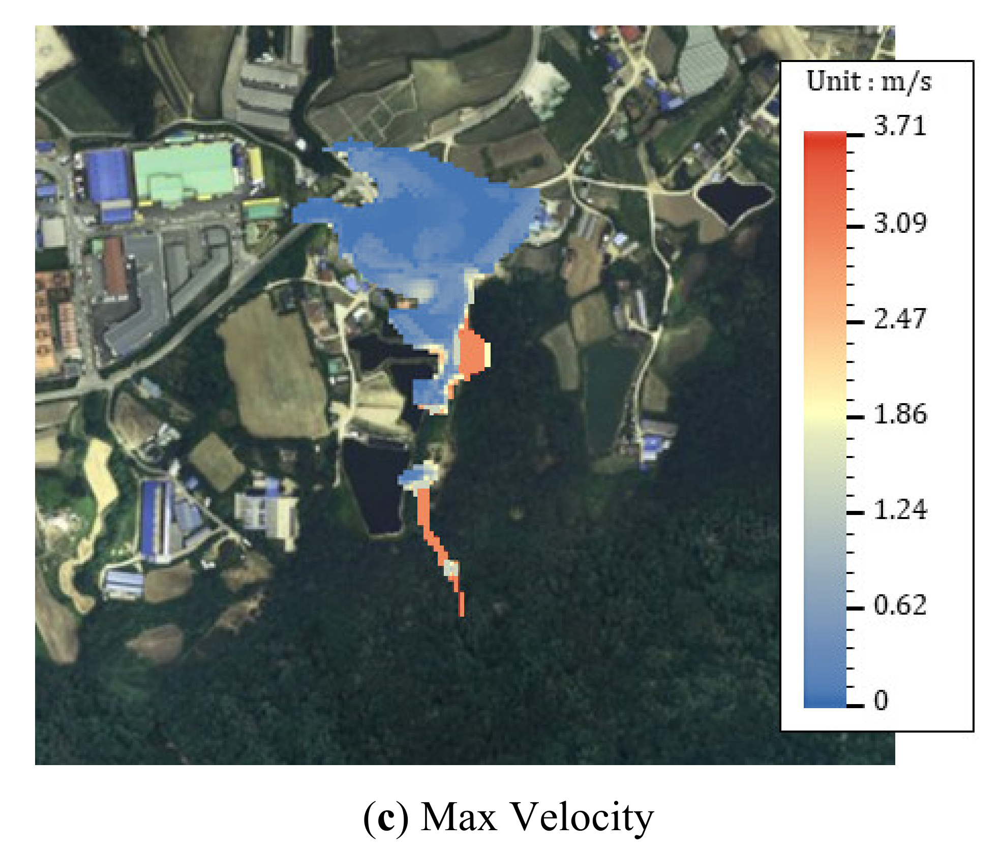
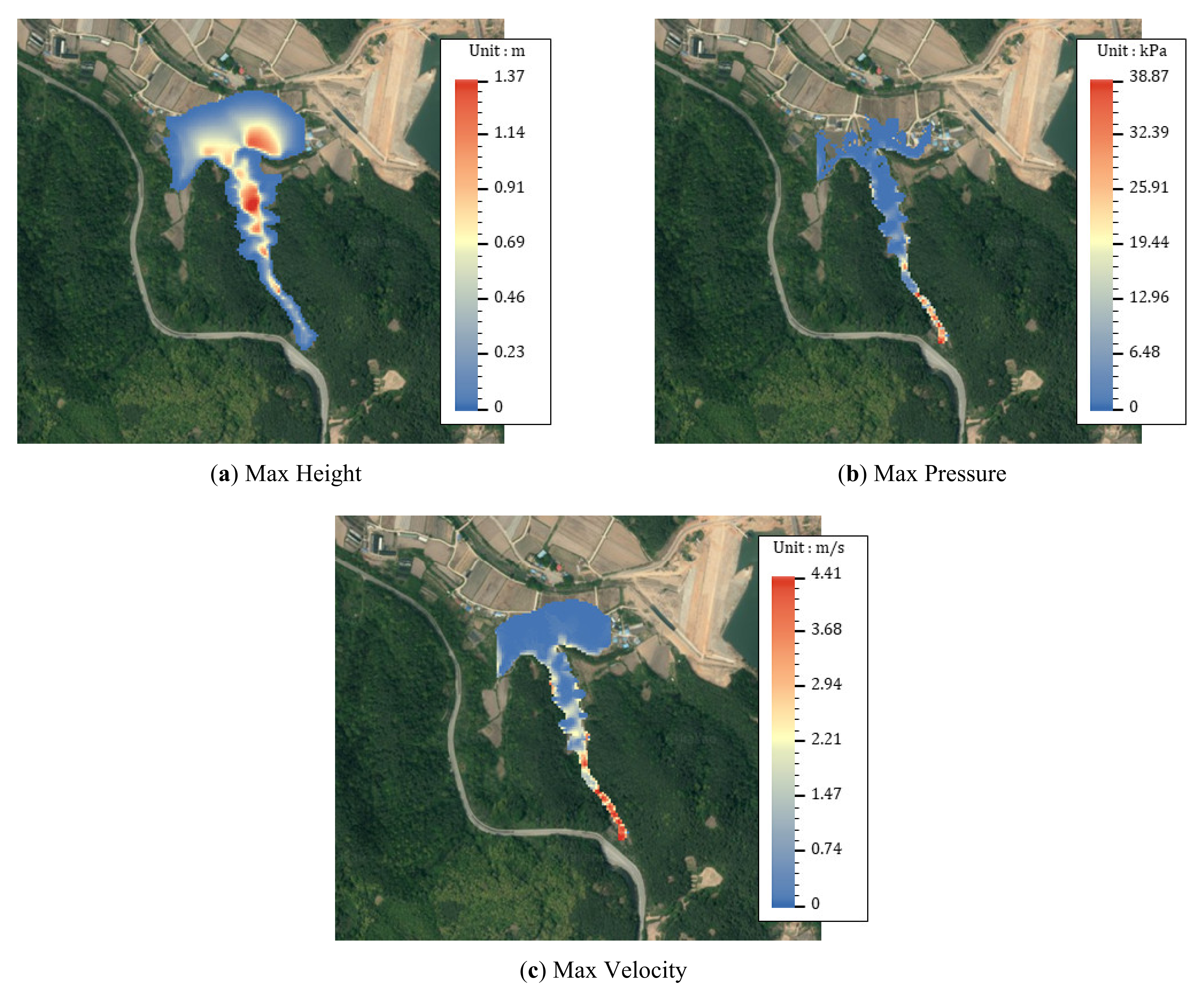
The peak runoff of the HQPF and the possible soil runoff volume () calculated with the S-RAT model and the soil volume equation were used to simulate debris flow with the RAMMS model (Table 3). In the RAMMS modeling process, the default value was used for the drag coefficient. In Event Ⅰ, the max height was 2.43 m, the max pressure was 42.68 kPa, and the max velocity was 4.62 m/s. In Event II, the max height was 0.66 m, the max pressure was 18.05 kPa, and the max velocity was 3 . In Event III, the max height was 1.32 m, the max pressure was 34.19 kPa, and the max velocity was 4.13 . The damage areas in Events I, II, and III were 62,550 , 56,325 , and 46,750 , respectively.
Displacement detection using GPS is not readily applicable to actual sites on account of the cost of installing automatic measuring instruments across the slope, the need for continuous maintenance, and the difficulties with management. The horizontal precision is ±1 cm and the vertical precision is ±2 cm, which is not sufficient to measure landslide displacements showing sensitive behaviors in millimeters [31]. For this reason, in this study, a damage area was defined by an area with a maximum flow depth of 3 cm or deeper. Figure 13, Figure 14 and Figure 15 show the debris flow simulation results for Events I, II, and III based on the RAMMS model, projected on the Arc Map 10.7 satellite map.
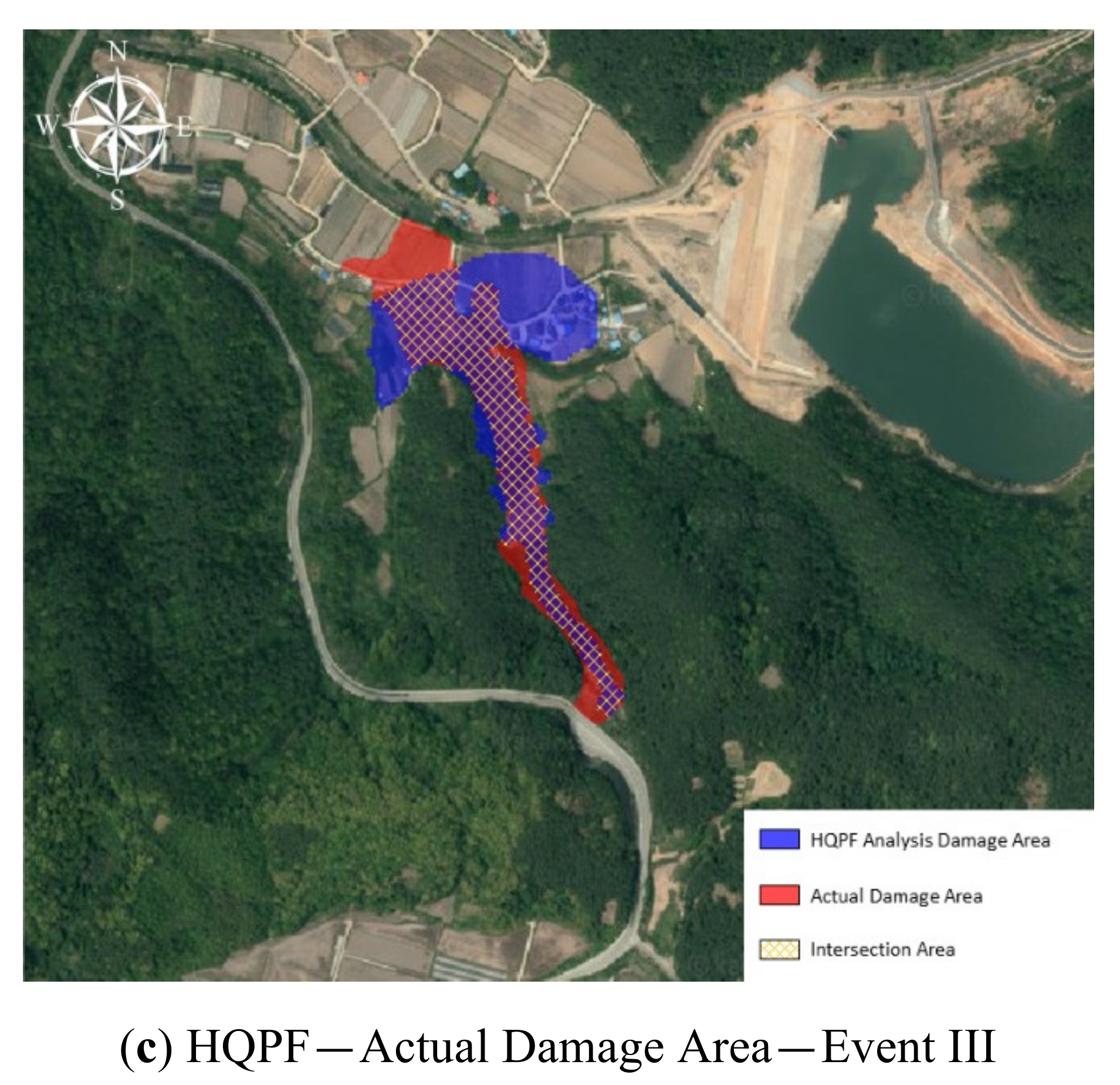
3.4. Verification of the Applicability of the HQPF Data Using Actual Damage Data
This study compared the flow damage scale data for each event based on the RAMMS model using the LSSI method. The LSSI method calculates the cross areas of measurement data corresponding to the reference data, thereby measuring the accuracy of spatial locations [32]. It divides the intersection area of two data group by the area of their union to calculate values in the form of standardized indexes in order to measure the correspondence of the spatial locations of the two groups of data. An index has a value between 0 and 1. A value closer to 1 indicates a higher level of correspondence between the two data groups, whereas a value closer to 0 indicates a low level of correspondence. In other words, the LSSI method offers a highly efficient way to measure the location accuracy of the reference data and the measurement data, to identify the spatial correspondence between the two. Hua et al. calculated LSSI indexes by comparing the city scope predicted in a urban growth simulation of coastal areas in China based on the slope, land cover, exclusion, urban growth, transport, and hill shade (SLEUTH) model, and the calculated city scopes [33]. It is difficult to achieve an LSSI index of 1, which means a perfect spatial correspondence. By comparing the predicted scopes with the city scopes after final correction, an LSSI index of 0.48 was achieved. Choi et al. compared the inundation patterns of the urban flooding model and the flood tracking model using the LSSI based on the flood trace map [34]. When the LSSI range is 40% or more, it is marked as excellent (40% or more—excellent; 30% or more—good; 20% or more—fair; 10% or more—poor; 5% or more—fail). Jung et al. investigated errors in cadastral maps and continuous cadastral maps using the LSSI index [32]. While the researchers failed to achieve a high LSSI value, the LSSI method proved to be useful.
The actual damage areas for Event I were identified based on the landslide investigation report in 2019 [35]. For Event II, the drone photographs taken by Kwon Wu-seong were used [36], and the damage areas for Event III were based on the drone photographs of the site by Jang Jeong-pil at the time of the event [37] (Figure 16).
The damage areas calculated based on the RAMMS model were compared, defined as areas with a maximum flow depth of 3 cm or deeper. Table 4 shows the LSSI analysis results of the damage areas calculated using the RAMMS model. Figure 17 is a projection of the damage areas based on the HQPF and the actual damage areas projected on an Arc map. The LSSI result for Event Ⅰ was 48.55%, which indicates a high degree of correspondence between the analyzed damage areas with the actual damage areas. The results for Events II and III were 44.70% and 44.88%, respectively, also indicating high levels of correspondence with the actual areas.
4. Conclusions
This study analyzed flow damage inflicted on Sinnam Village in Samcheok in October 2010, and Nansam Village in Anseong and Seongdeok Village in Gokseong in August 2020. HQPFs were generated by applying machine learning to precipitation data from KMA AWS near the damage sites, and the HQPFs were compared with the AWS data and the QPF. The data were applied to the damage areas after verification to generate HQPF. Then, the S-RAT model was used to calculate the damage areas, flow depths, and other damage scale parameters using the runoff volumes, soil volumes, and debris flow model for each event. The debris flow simulation results were also compared with the actual damage areas. The following paragraphs summarize the findings and conclusions of this study.
This study sought to create HQPFs of areas damaged by debris flow using machine learning. The calculated HQPFs were compared with QPFs, and the applicability of the HQPFs were verified by conducting a statistical QPF-AWS and HQPF-AWS verification and using a scatter plot for all three events.
The runoff volume for each event predicted in each area was calculated using the S-RAT model, and the calculated peak runoff and the soil volume were used along with the RAMMS model to analyze flow damage. The findings of the flow damage analysis based on the model are as follows. In Event Ⅰ, the max height was 2.43 m, the max pressure was 42.68 kPa, and the max velocity was 4.62 . In Event II, the max height was 0.66 m, the max pressure was 18.05 kPa, and the max velocity was 3 . In Event III, the max height was 1.32 m, the max pressure was 34.19 kPa, and the max velocity was 4.13 . The damage areas in Events I, II, and III were 62,550 , 56,325 , and 46,750 , respectively. The LSSI results indicated high levels of correspondence between the damage areas analyzed through the debris flow simulation using HQPF and the actual damage areas, with an average LSSI value of 46%.
The analysis of the runoff volumes and the flow damage using precipitation data confirmed that the HQPFs were well corrected. The debris flow analysis revealed differences in damage patterns and scales depending on the volume and pattern of rainfall, and the HQPFs seem to be applicable to the RAMMS model.
This study showed that machine learning offers an effective way to correct qualitative hydrological precipitation data, and also confirmed the applicability of HQPFs to debris flow analysis using the RAMMS model. Numerous studies have analyzed debris flows using past rainfall events. However, few studies have used precipitation forecasts to analyze debris flows and predict damages. The calculation of corrected precipitation forecasts and debris flow analysis based on debris flow models allows for the prediction of, and preparation against, possible damages in areas with debris flow risks. The authors will advance the prediction factors and machine learning methods further to predict and analyze debris flows highly affected by precipitation, and assess the applicability to debris flow simulation models other than the RAMMS model.
Author Contributions
All the authors contributed to the conception and development of this manuscript. C.-H.O. contributed to Coneptualization, Formal analysis and original writing. K.-S.C. contributed to the formal analysis, survey of the previous research. J.-R.C. contributed to the development of prior research and methodology. C.-M.G. contributed to the development of the methodology and the software part. B.-S.K. suggested idea of study and helped in analyzing the results and reviewed the writing. All authors have read and agreed to the published version of the manuscript.
Funding
This research received no external funding.
Institutional Review Board Statement
Not applicable.
Informed Consent Statement
Not applicable.
Data Availability Statement
Not applicable.
Acknowledgments
This research was supported by a grant (20010162) of Regional Customized Disaster-Safety R&D Program funded by Ministry of Interior and Safety (MOIS, Korea). This paper work (or document) was financially supported by Ministry of the Interior and Safety as Human Resource Development Project in Disaster Management(C2001644-01-01).
Conflicts of Interest
The authors declare no conflict of interest.
References
- Kim, S. Long-term Comprehensive Water Resources Plan (2001~2020): Report = Water Vision 2020; Ministry of Construction and Transportation: Sejong City, Korea, 2000.
- National Institute of Forest Science. Things to Know About Landslides; National Institute of Forest Science Research Data No. 584. 2014. Available online: http://know.nifos.go.kr/book/search/DetailView.ax?sid=1&cid=163018 (accessed on 1 August 2021).
- Nam, D.H.; Lee, S.H.; Jeon, G.W.; Kim, B.S. A Study on the Debris Flow Movement and the Run-out Calculation Using the Coupling of Flood Runoff Model and Debris Flow Model. Crisisonomy 2016, 12, 131–143. [Google Scholar] [CrossRef]
- Choi, Y.N.; Lee, H.H. Characteristic Analysis and Prediction of Debris Flow-Prone Area at Daeryongsan. J. Korean Assoc. Geogr. Inf. Stud. 2018, 21, 48–62. [Google Scholar]
- Kim, S.E.; Baek, J.C.; Kim, G.S. Run-out Modeling of Debris Flows in Mt. Umyeon using FLO-2D. J. Civ. Environ. Eng. Res. 2013, 33, 965–974. [Google Scholar]
- Jun, G.W.; Oh, C.Y. Study on Risk Analysis of Debris Flow Occurrence Basin Using GIS. J. Korean Soc. Saf. 2011, 26, 83–88. [Google Scholar]
- Yun, W.J.; Kim, J.H.; Bae, D.H. Application on the Coupled Short-Term Precipitation-Stream Flow Forecast. J. Korea Water Resour. Assoc. 2004, 2004, 308–312. [Google Scholar]
- Lee, J.D.; Bae, D.H. A Study on the Short-term Forecast Method Using Land-Gauge Data. J. Korea Water Resour. Assoc. 2009, 2009, 1167–1171. [Google Scholar]
- Jung, J.S.; Kim, K.S. Rainfall Nowcasting with Multi-later Neural Network. J. Kroean Soc. Environ. Technol. 2000, 1, 95–100. [Google Scholar]
- Kim, G.S. Forecast of Areal Average Rainfall Using Radiosonde Data and Neural Networks. J. Korea Water Resour. Assoc. 2006, 39, 717–726. [Google Scholar] [CrossRef] [Green Version]
- Kim, G.S.; Kim, J.P. Development of a Short-term Rainfall Forecast Model Using Sequential CAPPI Data. J. Civ. Environ. Eng. Res. 2009, 29, 543–550. [Google Scholar]
- Yoon, S.S.; Bae, D.H.; Choi, Y.J. Urban Inundation Forecasting Using Predicted Radar Rainfall: Case Study. J. Korean Soc. Hazard. Mitig. 2014, 14, 117–126. [Google Scholar] [CrossRef] [Green Version]
- Kim, B.S.; Yun, S.G.; Yang, D.M.; Gwon, H.H. Development of Conceptually Grid Based Hydrological Model. J. Korea Water Resour. Assoc. 2010, 43, 667–679. [Google Scholar] [CrossRef]
- Jung, S.H.; Lee, D.E.; Lee, K.S. Prediction of River Water Level Using Deep-Learning Open Library. J. Korean Soc. Hazard. Mitig. 2018, 18, 1–11. [Google Scholar] [CrossRef]
- Choi, C.H.; Kim, J.S.; Kim, D.H.; Lee, J.H.; Kim, D.H.; Kim, H.S. Development of Heavy Rain Damage Prediction Functions in the Seoul Capital Area Using Machine Learning Techniques. J. Korean Soc. Hazard. Mitig. 2018, 18, 435–447. [Google Scholar] [CrossRef] [Green Version]
- Ham, Y.G.; Kim, J.H.; Luo, J.J. Deep Learning for ENSO forecasts. Nature 2019, 573, 568–572. [Google Scholar] [CrossRef] [PubMed]
- Fox, J.T.; Magoulick, D.D. Predicting hydrologic disturbance of streams using species occurrence data. J. Sci. Total Environ. 2019, 686, 254–263. [Google Scholar] [CrossRef] [PubMed]
- Lee, Y.M.; Ko, C.M.; Shin, S.C.; Kim, B.S. The Development of a Rainfall Correction Technique based on Machine Learning for Hydrological Applications. J. Environ. Sci. Int. 2019, 28, 125–135. [Google Scholar] [CrossRef]
- Yen, M.H.; Liu, D.W.; Hsin, Y.C.; Lin, C.E.; Chen, C.C. Application of the deep learning for the prediction of rainfall in Southern Taiwan. Sci. Rep. 2019, 9, 12774. [Google Scholar] [CrossRef] [Green Version]
- Korea Meteorological Administration. Forecast Technologies in Your Hands; Korea Meteorological Administration Forecast Bureau: Seoul, Korea, 2012; p. 17. Available online: http://www.kma.go.kr/down/e-learning/hands/hands_17.pdf (accessed on 15 August 2021).
- Yoo, J.E. Random forests: An alternative data mining technique to decision tree. J. Educ. Eval. 2015, 28, 427–448. [Google Scholar]
- Choi, C.H.; Park, K.H.; Park, H.K.; Lee, M.J.; Kim, J.S.; Kim, H.S. Development of Heavy Rain Damage Prediction Function for Public Facility Using Machine Learning. J. Korean Soc. Hazard. Mitig. 2017, 17, 443–450. [Google Scholar] [CrossRef]
- Breiman, L. Random forests. Mach. Learn. 2001, 45, 5–32. [Google Scholar] [CrossRef] [Green Version]
- Houtao, D.; Runger, G.; Tuv, E. System monitoring with real-time contrasts. J. Qual. Technol. 2012, 44, 9–27. [Google Scholar]
- Nam, D.H.; Ha, H.J.; Kim, B.S. Validation of Flood Runoff Sumulation Using Distributed Hydrologic Models. J. Korean Soc. Hazard. Mitig. 2020, 20, 173–184. [Google Scholar] [CrossRef] [Green Version]
- Nam, D.H.; Kim, M.I.; Kang, D.H.; Kim, B.S. Debris Flow Damage Assessment by Considering Debris Flow Direction and Direction Angle of Structure in South Korea. Water 2019, 11, 328. [Google Scholar] [CrossRef] [Green Version]
- Hussin, H.Y.; Quan Luna, B.; Van Westen, C.J.; Christen, M.; Malet, J.-P.; Van Asch, T.H.W.J. Parameterization of a numerical 2-D debris flow model with entrainment: A Event study of the Faucon catchment, Southern French Alps. Nat. Hazards Earth Syst. Sci. 2012, 12, 3075–3090. [Google Scholar] [CrossRef]
- Takahashi, T.; Nakagawa, H.; Satofuka, Y.; Kawaike, K. Flood and sediment disasters triggered by 1999 rainfall in VeneZuela: A river restoration plan for an alluvial fan. J. Nat. Disaster Sci. 2001, 23, 65–82. [Google Scholar]
- Hutter, K.; Svendsen, B.; Rickenmann, D. Debris flow modeling:A review. Contin. Mech. Thermodyn. 1994, 8, 1–35. [Google Scholar] [CrossRef]
- National Institute for Land and Infrastructure Management (NILIM). Manual of Technical Standard for Establishing Sabo Master Plan for Debris Flow and Driftwood; Technical Note of National Institute for Land Infrastructure Management No. 364; NILIM: Tsukuba, Japan, 2016; pp. 25–32. Available online: http://www.nilim.go.jp/lab/bcg/siryou/tnn/tnn0904pdf/ks0904.pdf (accessed on 1 August 2021).
- Chae, B.G.; Song, Y.S.; Choi, J.H.; Kim, G.S. The Current Methods of Landslide Monitoring Using Observation Sensors for Geologic Property. J. Sens. Sci. Technol. 2015, 24, 291–298. [Google Scholar] [CrossRef] [Green Version]
- Jung, G.H.; Jun, C.M.; Ko, J.H.; Park, Y.R. A Study on the Error Detection of Attached Cadastral Maps Using GIS. Proc. Korean Soc. Surv. Geod. Photogramm. Cartogr. Conf. 2007, 12, 47–55. Available online: https://www.koreascience.or.kr/article/CFKO200716419439853.jsp-kj=SSMHB4&py=2012&vnc=v27n6&sp=588 (accessed on 15 August 2021).
- Hua, L.; Tang, L.; Cui, S.; Yun, K. Simulating Urban Growth Using the SLEUTH Model in a Coastal Peri-Urban District in China. Sustainability 2014, 6, 3899–3914. [Google Scholar] [CrossRef] [Green Version]
- Choi, J.H.; Jeon, J.H.; Kim, T.H.; Kim, B.S. Comparison of inundation patterns of urban inundation model and flood tracking model based on inundation traces. J. Korea Water Resour. Assoc. 2021, 54, 71–80. [Google Scholar]
- Korea Forest Service. 2019 Landslide Cause Investigation Results Report; Korea Forest Service: Daejeon, Korea, 2019; pp. 28–53.
- Kwon, W.S. Oh My Photo 2020. The Scene of the ‘Disastrous Anseong Juksan-Myeon Landslide’ Seen with a Drone. Available online: http://www.ohmynews.com/NWS_Web/OhmyPhoto/2020/at_pg.aspx?CNTN_CD=A0002664401 (accessed on 15 August 2021).
- Jin, C.I. JoongAng Ilbo. Gokseong Landslide Disastrous for 5 People… Residents: “Soil Collapsed at the National Road Expansion Construction Site”. Available online: https://www.joongang.co.kr/article/23844086#home (accessed on 15 August 2021).
Figure 1.
Research flow chart of hydrological cycle change in North Korea.

Figure 2.
Concept of random forest.

Figure 3.
Grid type water balance calculation concept diagram [13].
Figure 3.
Grid type water balance calculation concept diagram [13].

Figure 4.
A schematic interpretation of the RAMMS Model.

Figure 5.
Analyzed areas. (a) Samcheok, Gangwon-do, (b) Anseong, Gyeonggi-do, (c) Gokseong, Jeollanam-do.
Figure 5.
Analyzed areas. (a) Samcheok, Gangwon-do, (b) Anseong, Gyeonggi-do, (c) Gokseong, Jeollanam-do.

Figure 6.
Schematic diagram of machine learning.

Figure 7.
Location of the Station. (A) Gungchon station, (B) Samjuk Elementary School station, and (C) Ogwa Tollgate station.
Figure 7.
Location of the Station. (A) Gungchon station, (B) Samjuk Elementary School station, and (C) Ogwa Tollgate station.

Figure 8.
Precipitation Forecast at Nearby Precipitation Observation Stations. (a) Hyetograph of Gungchon Station, (b) 24-hour cumulative rainfall of Gungchon Station, (c) Hyetograph of Samjuk Elementary School Station, (d) 24-hour cumulative rainfall of Samjuk Elementary School Station, (e) Hyetograph of Okwa Tollgate, and (f) 24-hour cumulative rainfall of Okwa Tollgate. In each graph, black means AWS Rainfall, blue means QPF, and red means HQPF.


Figure 9.
Scatter Plots of the Correlation between AWS-QPF and AWS-HQPF (Events I, II, and III).

Figure 10.
Hyetograph of the Study Area. (a) Hyetograph of Sinnam Village, (b) 24-hour cumulative rainfall of Sinnam Village, (c) Hyetograph of Namsan Village, (d) 24-hour cumulative rainfall of Namsan Village, (e) Hyetograph of Sungdeok Village, (f) 24-hour cumulative rainfall of Sungdeok Village. In the bar graphs of (a,c,e), blue is QPF Rainfall and red is HQPF Rainfall. In the solid line graphs of (b,d,f), blue is QPF and red is It means HQPF, and the dots marked for each hour mean the accumulated rainfall for that time.

Figure 11.
GIS Input Data for the S-RAT. (a–f) S-RAT input data of Event I Sinnam Village, (g–l) S-RAT input data of Event II Namsan Village, (m–r) S-RAT input data of Event III Sungduk Village.
Figure 11.
GIS Input Data for the S-RAT. (a–f) S-RAT input data of Event I Sinnam Village, (g–l) S-RAT input data of Event II Namsan Village, (m–r) S-RAT input data of Event III Sungduk Village.


Figure 12.
Runoff-Rainfall Graphs of QPF and HQPF. (a) is the Runoff-Rainfall graph of Event Ⅰ Sinnam Village, (b) is the Runoff-Rainfall graph of Event II Namsan Village, (c) is the Runoff-Rainfall graph of Event III Sungduk Village. Where the blue bar graph is QPF Rainfall, the red bar graph is the HQPF rainfall, the blue solid line is the QPF runoff, and the red solid line is the HQPF runoff.

Figure 13.
Results of RAMMS using HQPF—Event I. (a–c) are the Max Height (), Max Pressure (), and Max Velocity () in the modeling results of the debris flow in Sinnam Village, respectively.
Figure 13.
Results of RAMMS using HQPF—Event I. (a–c) are the Max Height (), Max Pressure (), and Max Velocity () in the modeling results of the debris flow in Sinnam Village, respectively.

Figure 14.
Results of RAMMS using HQPF—Event II. (a–c) are the Max Height (), Max Pressure (), and Max Velocity () in the modeling results of the debris flow in Namsan Village, respectively.
Figure 14.
Results of RAMMS using HQPF—Event II. (a–c) are the Max Height (), Max Pressure (), and Max Velocity () in the modeling results of the debris flow in Namsan Village, respectively.


Figure 15.
Results of RAMMS using HQPF—Event III. (a–c) are the Max Height (), Max Pressure (), and Max Velocity () in the modeling results of the debris flow in Sungduk Village, respectively.
Figure 15.
Results of RAMMS using HQPF—Event III. (a–c) are the Max Height (), Max Pressure (), and Max Velocity () in the modeling results of the debris flow in Sungduk Village, respectively.

Figure 16.
Damaged area in the literature. (a) is the 2019 Landslide Investigation Report, (b) is drone video and photos taken by Kwon Wu-seong, and (c) is the status of each debris flow area referring to the article by reporter Jin Chang-il of the JoongAngIlbo.
Figure 16.
Damaged area in the literature. (a) is the 2019 Landslide Investigation Report, (b) is drone video and photos taken by Kwon Wu-seong, and (c) is the status of each debris flow area referring to the article by reporter Jin Chang-il of the JoongAngIlbo.


Figure 17.
LSSI analysis results. In (a–c), the area marked in blue is the HQPF Analysis Damage Area, and the area marked in red is the actual damage area. And the area marked with a yellow checkered pattern means the part where the HQPF Analysis Damage Area and the actual damage area intersect.
Figure 17.
LSSI analysis results. In (a–c), the area marked in blue is the HQPF Analysis Damage Area, and the area marked in red is the actual damage area. And the area marked with a yellow checkered pattern means the part where the HQPF Analysis Damage Area and the actual damage area intersect.


Table 1.
Statistical Verification of QPF and HQPF (Events I, II, and III).
| Verification | Event I | Event II | Event III | |||
|---|---|---|---|---|---|---|
| QPF-AWS | HQPF-AWS | QPF-AWS | HQPF-AWS | QPF-AWS | HQPF-AWS | |
| MAE | 11.78 | 5.65 | 10.57 | 4.1 | 20.03 | 5.93 |
| NPE | −0.73 | −0.38 | 0.27 | 0.47 | 1.2 | 0.2 |
| PTE | 0 | 0 | −6 | 0 | 8 | 4 |
Table 2.
Input variables required to calculate soil runoff volume.
| Event I | Event II | Event III | |
|---|---|---|---|
| Solid density () | |||
| Liquid density () | |||
| Internal friction angle () | |||
| Average slope () | |||
| Equilibrium sediment concen-tration () | 0.32 | 0.41 | 0.31 |
| Porosity () | 0.45 | 0.45 | 0.45 |
| Cumulative rainfall () | |||
| Basin Area () | |||
| Runoff correction rate () | 0.26 | 0.439 | 0.493 |
| Soil runoff volume () |
Table 3.
Debris Flow Simulation Results Using the RAMMS Model.
| Event I | Event II | Event III | |
|---|---|---|---|
| Max Height | |||
| Max Pressure | |||
| Max Velocity | |||
| Damage Area |
Table 4.
LSSI analysis of damage area calculated through RAMMS.
| Event I | Event II | Event III | |
|---|---|---|---|
| Actual Damage Area (A) | |||
| Analysis Damage Area (B) | |||
| 48.55% | 44.70% | 44.88% |
Publisher’s Note: MDPI stays neutral with regard to jurisdictional claims in published maps and institutional affiliations. |
© 2021 by the authors. Licensee MDPI, Basel, Switzerland. This article is an open access article distributed under the terms and conditions of the Creative Commons Attribution (CC BY) license (https://creativecommons.org/licenses/by/4.0/).
Share and Cite
MDPI and ACS Style
Oh, C.-H.; Choo, K.-S.; Go, C.-M.; Choi, J.-R.; Kim, B.-S. Forecasting of Debris Flow Using Machine Learning-Based Adjusted Rainfall Information and RAMMS Model. Water 2021, 13, 2360. https://doi.org/10.3390/w13172360
AMA Style
Oh C-H, Choo K-S, Go C-M, Choi J-R, Kim B-S. Forecasting of Debris Flow Using Machine Learning-Based Adjusted Rainfall Information and RAMMS Model. Water. 2021; 13(17):2360. https://doi.org/10.3390/w13172360
Chicago/Turabian StyleOh, Cheong-Hyeon, Kyung-Su Choo, Chul-Min Go, Jung-Ryel Choi, and Byung-Sik Kim. 2021. "Forecasting of Debris Flow Using Machine Learning-Based Adjusted Rainfall Information and RAMMS Model" Water 13, no. 17: 2360. https://doi.org/10.3390/w13172360
Note that from the first issue of 2016, this journal uses article numbers instead of page numbers. See further details here.