
A Study on the Flux of Total Suspended Matter in the Padma River in Bangladesh Based on Remote-Sensing Data

1
State Key Laboratory of Satellite Ocean Environment Dynamics, Second Institute of Oceanography, MNR, Hangzhou 310012, China
2
Marine Resources Big Data Center of South China Sea, Southern Marine Science and Engineering Guangdong Laboratory, Zhanjiang 524088, China
3
National Earth System Science Data Center, Beijing 100101, China
*
Author to whom correspondence should be addressed.
Water 2021, 13(17), 2373; https://doi.org/10.3390/w13172373
Submission received: 14 July 2021
/
Revised: 23 August 2021
/
Accepted: 26 August 2021
/
Published: 29 August 2021
(This article belongs to the Section Oceans and Coastal Zones)
Abstract
:The flux of total suspended matter (TSM), FTSM, output by several large rivers in Asia, has been in decline due to human activities. As the estuary of the Ganges–Brahmaputra River, the Padma River transports a significant amount of suspended matter (SM) to the Bay of Bengal each year. In this study, the TSM concentration (CTSM) and FTSM in the Padma River in the period 1991–2019 were calculated based on the data acquired by the Landsat series satellites and an empirical TSM algorithm model for large, high-turbidity rivers. The results showed that the maximum and minimum FTSM values (318 ± 62 and 73 ± 29 mt, respectively) in the Padma River occurred in 2011 and 2015, respectively. On average, FTSM in the Padma River decreased at an annual rate of 3.3 mt (p < 0.01). The impact of human activities on CTSM contributed more significantly to the changes in FTSM (R = 0.76) than natural factors (R = 0.44). Due to a lack of water conservancy facilities within the river basin, changes in the water and soil retention capacity due to the changes in vegetation coverage were an important human factor (R = −0.79).
1. Introduction
Total suspended matter (TSM) is an important index for evaluating the water quality in water bodies. In water-quality management, both the concentration and flux of TSM (CTSM and FTSM, respectively) depend on the gross primary productivity, the concentration of heavy metals, and the flux of substances such as radionuclides and organic micropollutants [1]. The concentration of total suspended matter, similarly, has a significant impact on the biogeochemical properties of coastal oceanic waters. The presence of TSM reduces the underwater transmittance of a water body [2] and alters its optical properties. For inland water bodies (e.g., rivers and lakes), TSM also plays a substantial role in maintaining ecosystem equilibrium and controlling the habitat of aquatic organisms. The CTSM value in a water body can help to maintain its ecosystems only when controlled within a suitable range. For example, an extremely high CTSM may cause wear damage to the eggs of aquatic organisms or directly lead to the death of their larvae [3]. On the other hand, some prey fish can evade their natural enemies by taking advantage of turbid water [4,5]. In addition, TSM and sediment can provide the environments and nutrients needed for the development of estuarine ecosystems.
Monitoring and studying the changes in the flux of TSM in large rivers is currently a focus area for research. Recent studies have shown that the flux of SM transported by large deltaic rivers is in decline, especially in Asia [6]. The transfer of both water and sediment to the sea will decrease as more dams and other river projects are built and utilized [7]. In the past 60 years, the flux of sediment transported seaward by the nine major rivers in China [8] as well as the Mekong River [9] have shown a statistically significant negative trend due to the construction of reservoirs. At present, the traditional calculation methods of FTSM are mainly based on measured hydrological data [8], hydrological climate model [9], isotope analysis [10], UAV measurement [11], and so on. The above method has the disadvantages of a large amount of calculation, difficult data acquisition, and excessive research cost [12]. In large tropical rivers such as Padma River, the installation and maintenance of in situ stations is a very costly task, limiting the data available for both river discharge and sediment load trend assessment. For these reasons, assessment of FTSM in large rivers by remote sensing monitoring has received increasing interest from the scientific community [13]. As an efficient, low-cost, long-term indirect observation technique, remote sensing plays a vital role in several research fields including hydrology.
The Padma River is the estuary of the Ganges–Brahmaputra River. Glacial meltwater from the Tibetan Plateau, known as the “Asian Water Tower”, is a primary source of freshwater for the Ganges–Brahmaputra River [14]. After converging in the Padma River, the water in the Ganges–Brahmaputra River flows into the Bay of Bengal, significantly affecting the eco-environmental changes in its northern waters. Many researchers have conducted relevant studies on the water constituents in the northern Bay of Bengal, including the measurement and monitoring of parameters such as the concentration of heavy metals [15], nutrients [16], dissolved oxygen [17], chlorophyll [18], and sediment [19]. Other researchers have observed this region over a large area through satellite remote sensing [20]. However, to date, few studies have monitored and estimated the flux of SM at the mouth of the Ganges River based on high-resolution satellite remote-sensing data.
2. Materials and Methods
2.1. Study Area
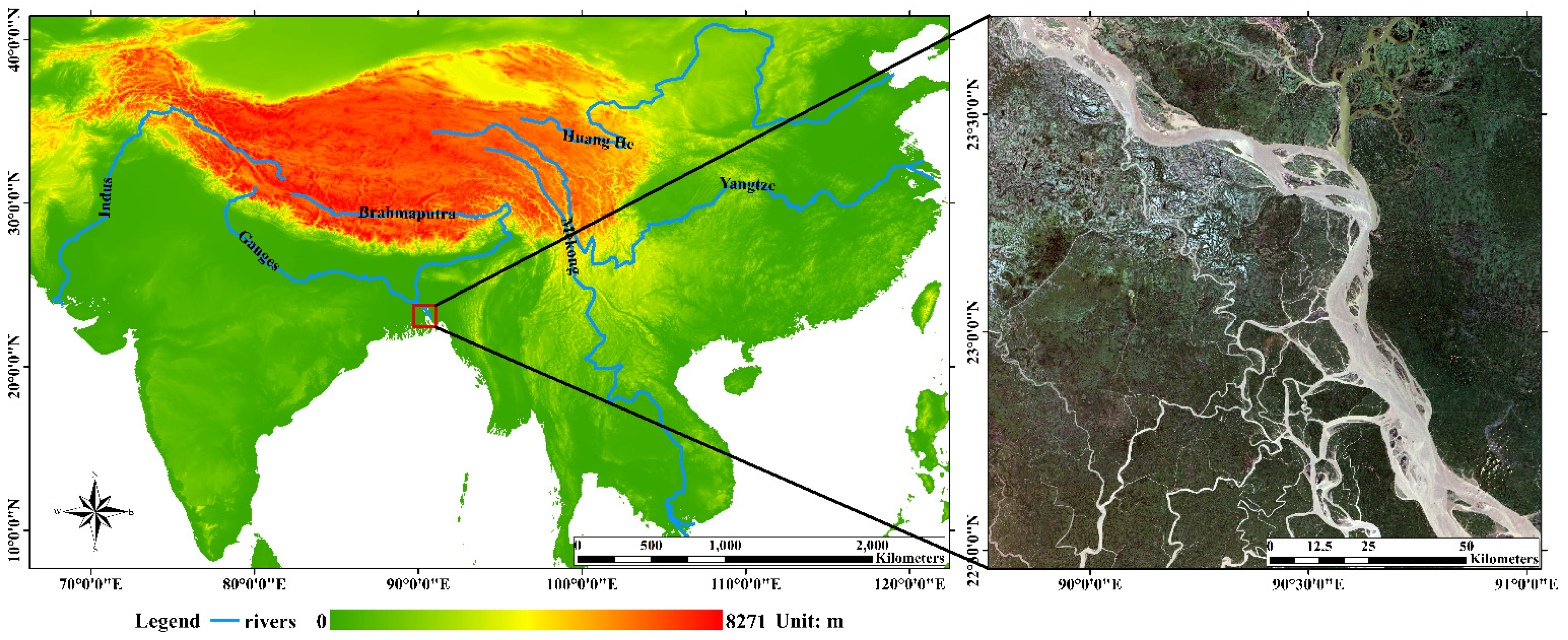
The Padma River is the estuary of the Ganges–Brahmaputra River. The estuaries of three large rivers, namely, the Ganges, the Brahmaputra, and the Meghna, flow into the Bay of Bengal through Padma River (see Figure 1). Each year, the Ganges–Brahmaputra river system, which has the world’s largest annual sediment discharge, approximately 100 billion tons [21,22], transports a significant amount of freshwater and SM into the Bay of Bengal [23]. The northern Bay of Bengal is home to the world’s largest mangrove forest—the Sundarbans—which discharges 18 million tons of SM and organic matter into the Bay of Bengal via various small tributaries, resulting in a complex ecosystem in the coastal waters of the northern Bay of Bengal [24].
The Padma River—a main tributary of the Ganges River—converges in the downstream region with the Meghna River—a tributary of the Brahmaputra River—and eventually flows into the Bay of Bengal. Since 1966, approximately 660 km2 of land have been eroded by the Padma River [25].
2.2. Hydrological Data
The reanalysis data used in this study included discharge and precipitation. The discharge data originated from the global modelled daily river discharge data from the Global Flood Awareness System [26]. Specifically, the monthly mean discharge data for the period 1991–2019 with the resolution 0.1° × 0.1° were used. There were a total of 348 data records.
The precipitation data originated from the Global Precipitation Climatology Project [27], which is a satellite precipitation product (resolution: 0.5° × 0.5°) produced by the Global Precipitation Climatology Center through combining the infrared (IR) and microwave data acquired by dozens of geostationary and polar-orbit satellites and correcting the resulting data against the data acquired by multiple ground stations worldwide. Specifically, the monthly mean precipitation data (data format: netCDF4) for the period 1991–2019 were used in this study. There were a total of 348 data records.
The Bay of Bengal has a sub-tropical monsoon climate with high temperature all year round and distinct monsoon and non-monsoon seasons. The monsoon season is from May to October, and about 84% of the rainfall occurs from June to October. The precipitation is concentrated. In addition, the terrain is low and flat, and the drainage is not smooth, which is easy to lead to flood disasters. The dry season is from November to April. Affected by the northeast monsoon, there is drought and less precipitation. Meanwhile, the water in non-monsoon season is not enough to meet the requirements of irrigation and shipping, nor to maintain the minimum environmental flow of the river [28].
2.3. Remote-Sensing Data
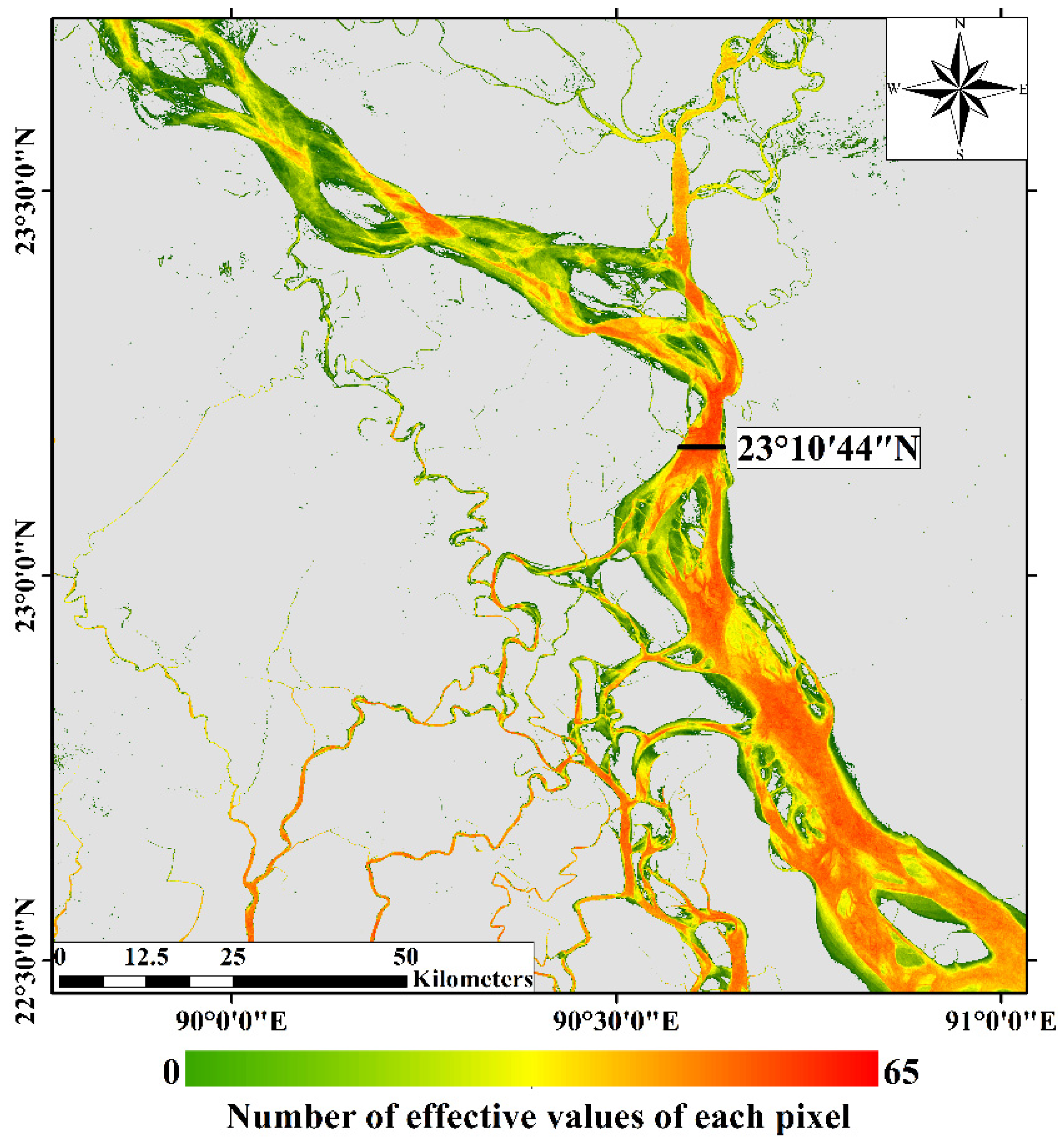
Landsat data, including Landsat-8 Operational Land Imager (OLI)/Thermal Infrared Sensor (TIRS) L1 products (resolution: 30 m) and Landsat-5 Thematic Mapper (TM) L1 products (resolution: 30 m), were used as experimental satellite data in this study. Sentinel-2 L2A reflectance products (resolution: 10 m) were used to perform spectral validation on the Landsat satellite data. These satellite data were downloaded from the official website of the United States Geological Survey (USGS) (https://earthexplorer.usgs.gov/ (accessed on 22 July 2020)). The Landsat products, covering the period from 1991 to 2019, provided images of the non-tidal reaches of the Padma River (row and column numbers: 137–044). At least one image was selected for each season. After the unusable data covered by cloud were removed, a total of 85 images were obtained. The number of effective values of each pixel can be seen in Figure 2.
The Landsat data used in this study were obtained from the official website of the USGS. Specifically, the L1 standard data (which had been geometrically corrected) were downloaded. In addition, the remote-sensing data were corrected based on the DEM data. Further, the following processes were performed to obtain more accurate reflectance data.
2.3.1. Radiometric Calibration
When remote-sensing data acquired at different times and locations or by different sensors are compared, it is necessary to convert the grey values of images to absolute radiance values to facilitate the calculation of the spectral reflectance or radiance of ground features [29]. In this study, radiometric calibration was performed using the Radiometric Calibration function within the Radiometric Correction tool in the ENVI 5.3 software package.
2.3.2. Atmospheric Correction
In this study, atmospheric correction was completed using the FLAASH Atmospheric Correction Model within the Radiometric Correction tool in the ENVI 5.3 software package. The FLAASH Atmospheric Correction Model, developed through improving the Moderate Resolution Atmospheric Transmission model, has relatively high accuracy in correcting hyperspectral and multispectral data [30]. Specifically, based on the geographical location of the study area, the Tropical Atmospheric Model and Maritime Aerosol Model were selected.
2.4. CTSM Inversion Model
The CTSM algorithm for the estuary of the Yangtze River developed by Liu et al. (2019) [31] was selected in this study for CTSM estimating based on the following considerations (see Table 1):
- The estuarian waters of both the Yangtze and Ganges Rivers are high in CTSM and contain TSM mostly from terrestrial sources [31].
- The estuaries of the Yangtze and Ganges Rivers are similar in terms of CTSM and the content ranges of main water constituents (e.g., chlorophyll) [18].
- The sensitive bands of the Landsat TM sensor for the TSM and main water constituents (e.g., chlorophyll) in both the estuaries of the Yangtze and Ganges Rivers are identical.
- The regions where the estuaries of the Yangtze and Ganges Rivers are located share the same rainy season. Therefore, high discharges and high CTSM values occur at the same time in the estuaries of the Yangtze and Ganges Rivers.
Thus, the algorithm developed by Liu et al. (2019) [31] is also applicable to the estuary of the Ganges River. The CTSM was calculated using the following algorithm:
where a and b are both fitting coefficients (a = 2.1454 and b = 0.2945 for Landsat-5 TM data; a = 2.1012 and b = 0.2953 for Landsat-7 Enhanced TM Plus (ETM+) data; the absolute relative errors for Landsat-5 TM and Landsat-7 ETM+ data are 13.69% and 13.46%, respectively) and band 4 and band 1 are the reflectance values of bands 4 and 1 of the Landsat-5/7 sensors, respectively.
2.5. M–K Test
The Mann–Kendall (M–K) test [33,34] is a climate diagnosis and prediction technique that can be used to determine whether an abrupt climate change occurred from a climate data series and, if so, its time of occurrence:
where is the value of the variable. A positive Z value suggests an upward trend in the variable, a negative Z value suggests a downward trend in the variable, and absolute Z values greater than 1.28, 1.64, and 2.32 signify the passing of significance tests at confidence levels of 90%, 95%, and 99%, respectively. The test result (i.e., Z value) reflects the overall trend of the variable.
The M–K abrupt-change test can be used to determine whether there exists an abrupt change. Similarly, for variable series , we define the following:
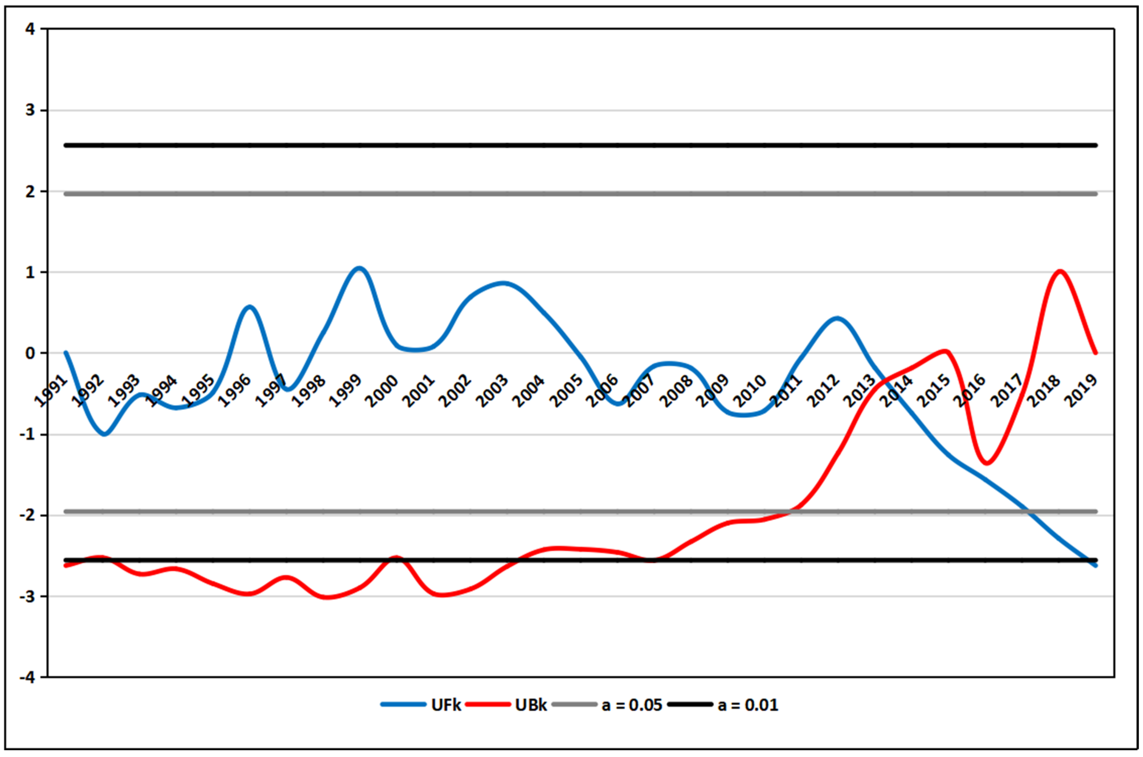
Then, whether there is an abrupt change in variable can be analyzed based on the two statistics UFk and UBk. The point of intersection of the UFk and UBk curves is the abrupt-change point. The UFk curve and UBk curve signify the sequential and reversed time series for xn, respectively. The critical values for the significance levels a = 0.05 and 0.01 (U0.05 and U0.01, respectively) are ±1.96 and ±2.32, respectively. If the UFk or UBk value is greater than 0, it means that the series exhibits an upward trend; otherwise, the series exhibits a downward trend. If the curves exceed the critical straight lines, this indicates a significant upward or downward trend. The time period for which the curves exceed the critical lines is determined as the time period of the abrupt change. The point of intersection between the UFk and UFk curves within the critical lines corresponds to the starting time of the abrupt change.
2.6. Validation of Landsat Data with Sentinel Data
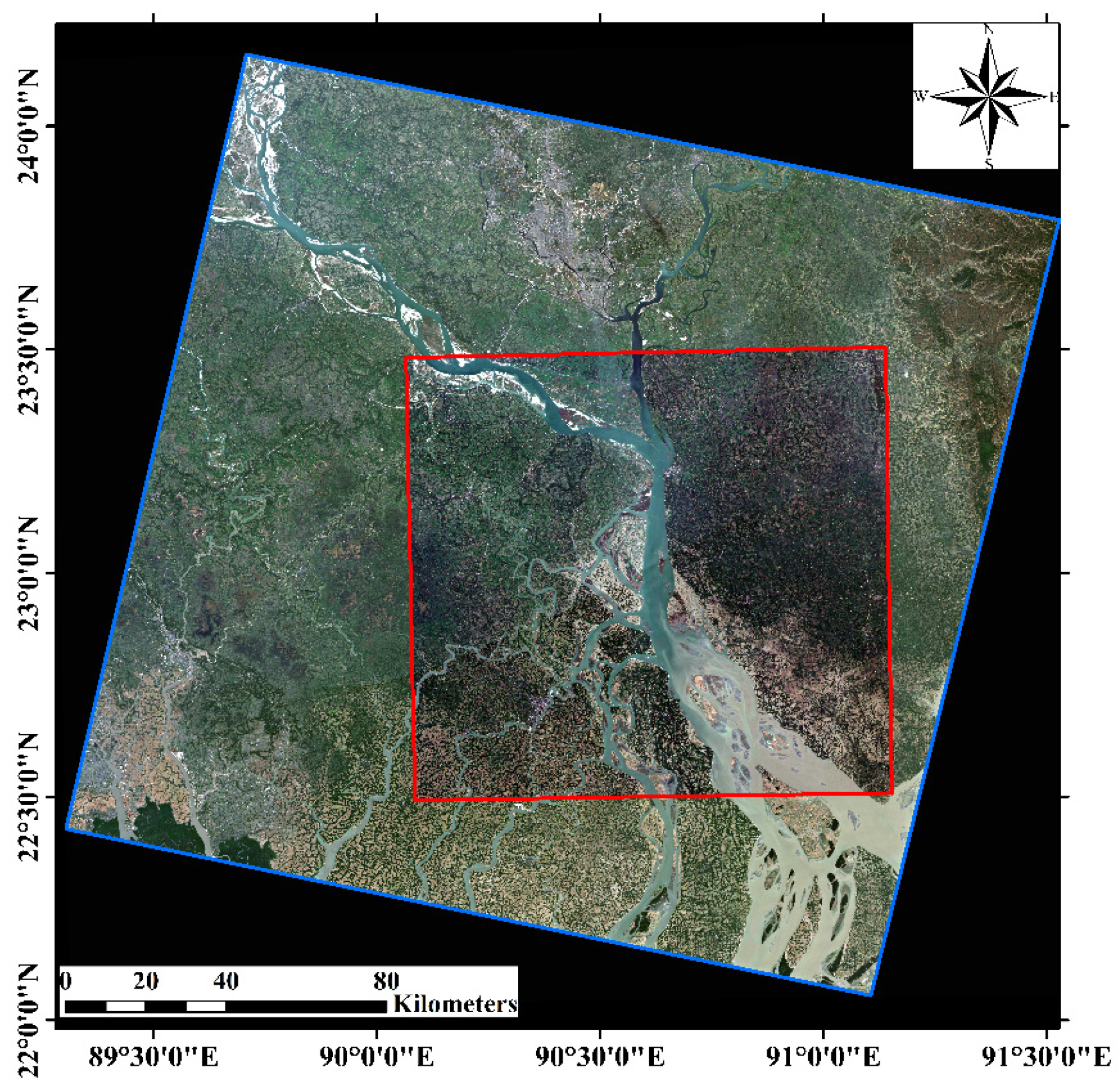
Sentinel-2 and Landsat-8 satellite data are extensively used in remote sensing of ocean colors. In addition, a large number of algorithms have been developed to integrate the data acquired by the sensors of these two satellites [35]. In this study, two Sentinel-2 L2A products were used to validate the atmospheric correction accuracy of the Landsat-8 data (see Figure 3). The two selected Sentinel-2 images were captured at 04:29:19 on 11 February 2020 and at 04:31:09 on 23 November 2019, respectively. The two corresponding Landsat-8 OLI/TIRS images were captured at 04:24:52 on 11 February 2020 and at 04:24:52 on 23 November 2019, respectively.
As mentioned above, the Landsat-8 OLI image was radiometrically calibrated and atmospherically corrected using the ENVI 5.3 software package. The image captured by the Multispectral Instrument (MSI) onboard the Sentinel-2 satellite was radiometrically calibrated and atmospherically corrected using the SNAP software. The difference between the OLI and MSI was eliminated using the sensor-transformation method developed by Zhang et al. (2018) [36] (see Table 3).
2.7. Normalized Difference Vegetation Index (NDVI)
The NDVI is an important parameter that reflects vegetation coverage and can be calculated for Landsat datasets using the equation [37]:
where and are the reflectance values in the NIR and red bands, respectively.
3. Results
3.1. Hydrology in the Study Area
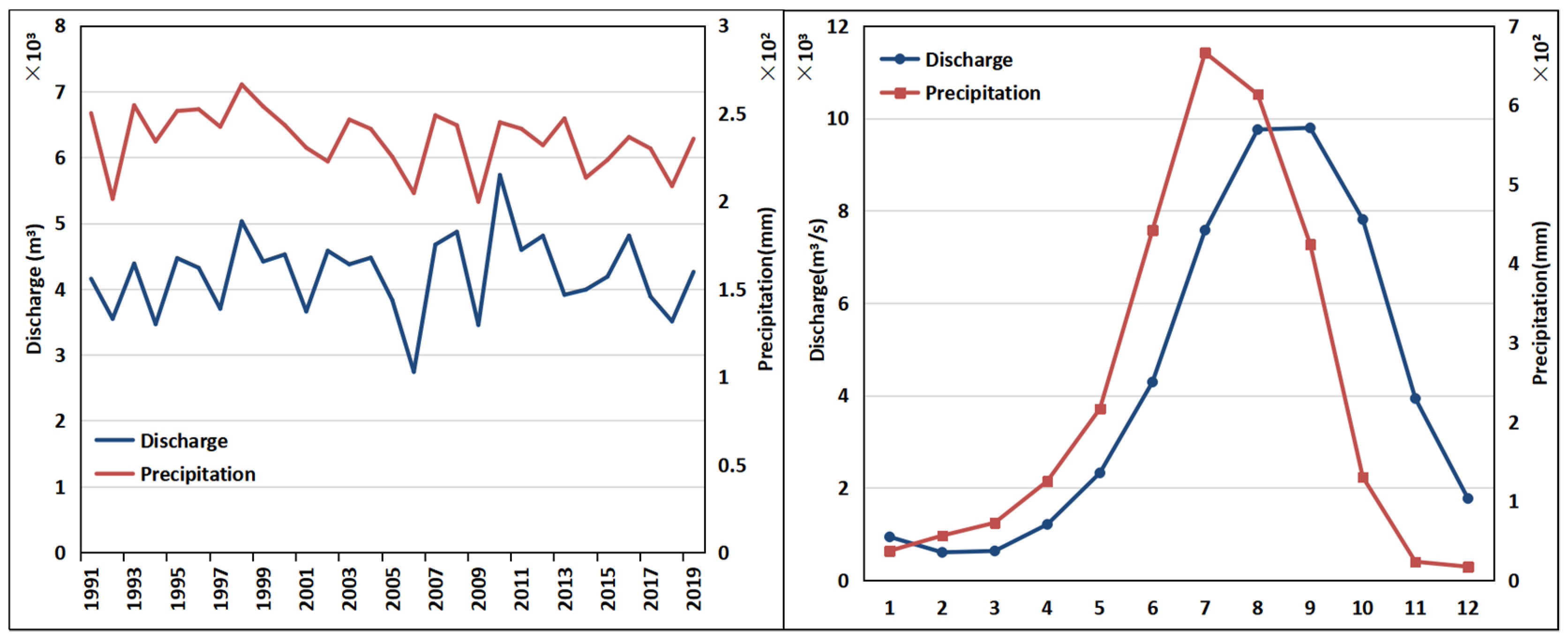
The changes of discharge and precipitation in the Padma River Basin during the study period are shown in Figure 4. The discharge result is calculated from GloFAS data, and the precipitation change result is calculated from GPCP data, which is the total precipitation in the basin. From May, precipitation and discharge begins to increase, and begins to decrease after October. From the change of monthly average results, the change of discharge lags the precipitation. The time-series data for the discharge and precipitation in the Padma River were analyzed using the M–K test. The Z value and its rate of change were obtained respectively (discharge: Z = 0.5730, slope = 1.4077 × 10⁸, p > 0.5; precipitation: Z = −1.2784, slope = 0.0375, p > 0.5). The results show that there is no obvious trend in discharge and precipitation in the past 30 years.
3.2. Comparison of Atmospheric Correction Results between Landsat and Sentinel
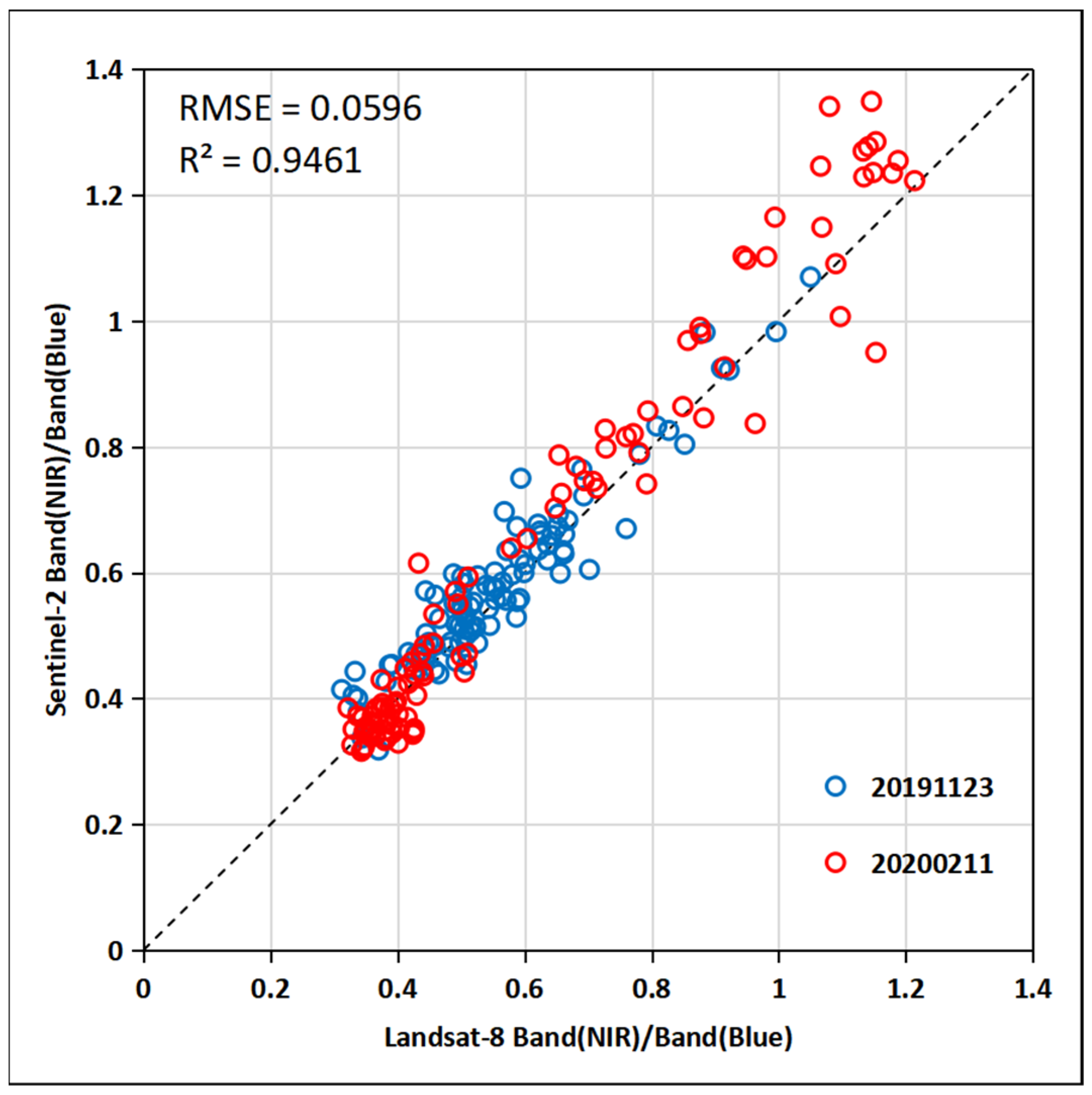
The NIR-band/blue-band ratio was calculated for points randomly selected within the river area, and the results were then compared. Similar ratios (R2 = 0.9563, root-mean-square error (RMSE) = 0.0811 in the 2020 image. R2 = 0.8963, RMSE = 0.0440 in the 2019 image. R2 = 0.9461, RMSE = 0.0596 in total) were obtained based on the data acquired by the two satellites (as shown in Figure 5), suggesting that the atmospherically corrected data were accurate and reliable.
3.3. Distribution of CTSM in the Padma River
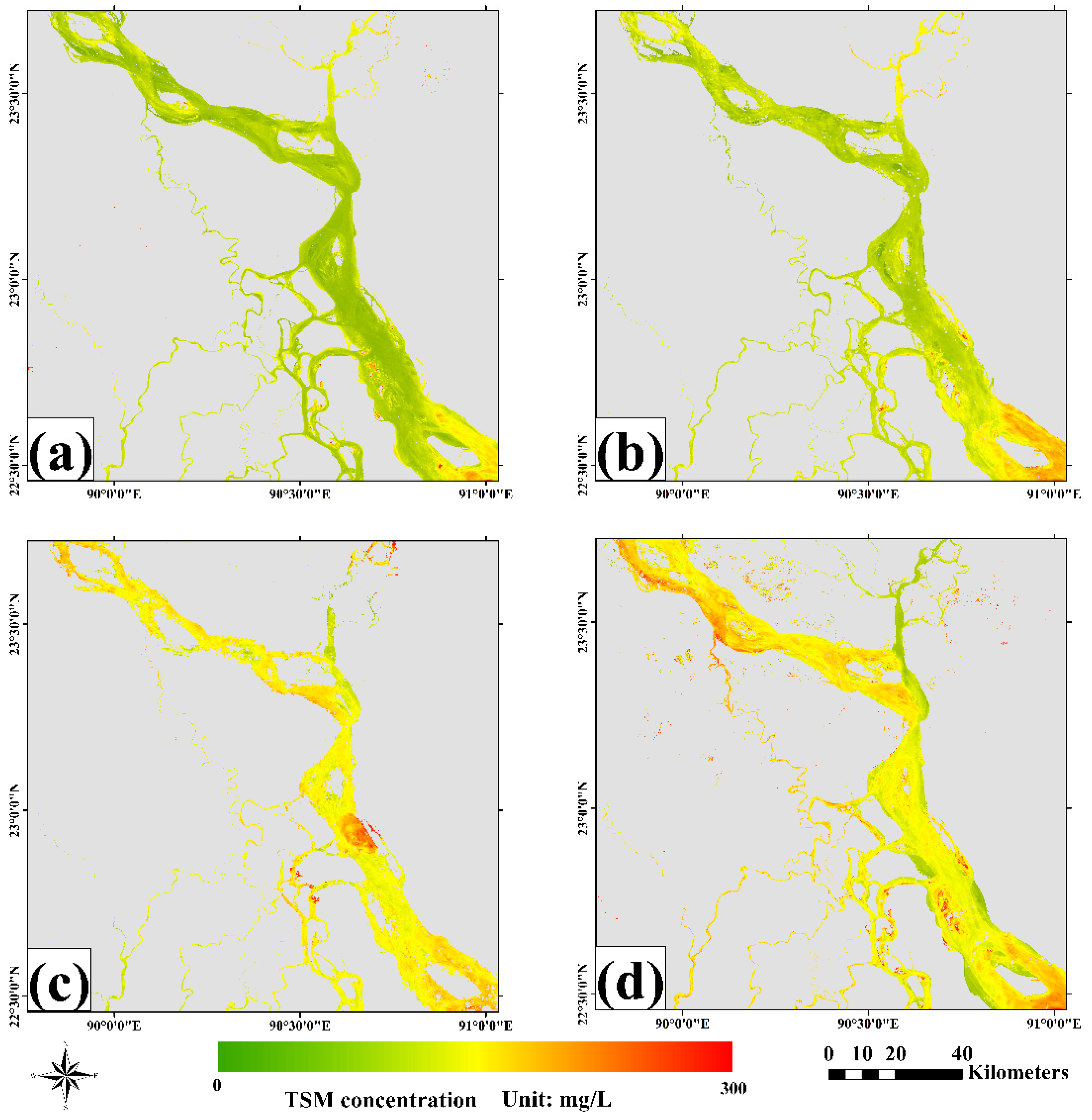
The arithmetic mean CTSM was calculated for each season of each year in the period 1991–2019. On this basis, the seasonal distribution of CTSM in the Padma River was obtained, as shown in Figure 6. In terms of the distribution trend, CTSM in the Padma River was high in areas close to the banks and in the downstream region and low in areas away from the banks and in the upstream region. The waters with relatively high CTSM values were distributed near the estuary in the downstream region, which was primarily due to the water and soil loss on the islands near the mouth of the estuary caused by the scouring of the water flow in the river as well as the convergence and resuspension of the matter (e.g., sediment) carried here by the water flow in the river from the upstream region. At a seasonal scale, CTSM was the lowest in winter (December through February of the following year). The CTSM remained below 150 mg/L in most parts of the river but reached up to 180 mg/L in some tributaries and 200 mg/L in the downstream region. There was a certain increase in CTSM in spring (March through May). Compared to winter, CTSM in spring exhibited an overall similar distribution trend but was higher in magnitude. The study area has a tropical monsoon climate with abundant precipitation in summer. Due to heavy precipitation and a large discharge, CTSM displayed a relatively uniform distribution pattern and, overall, remained at a relatively high level in summer (June through August). As a result of the soil erosion caused by precipitation and high flow rates, high CTSM values were distributed along both banks of the river and in the inland tributaries. The CTSM in the river was almost above 150 mg/L. In addition, due to an increase in the discharge, the erosion and siltation zone at the mouth of the estuary shifted outward. Similar to summer, CTSM in fall (September through November) remained above 150 mg/L in the main parts of the river, and high-CTSM zones shifted downstream.
3.4. Interannual Variations of CTSM in the Padma River
After the waters were separated from the land in the images, CTSM in the waters was estimated using the algorithm equation introduced in Section 2.4. The arithmetic means of the pixels in each image of the section showed in Figure 2 was calculated to represent the mean CTSM.
We also used Sentinel-2 data to calculate CTSM from 2016 to 2019 based on the same algorithm. In order to ensure the consistency of the algorithm, the reflectance data of Sentinel-2 were converted to the reflectance bands of Landsat-8 OLI by using the equation in Table 3, and then converted to the reflectance bands of Landsat-7 ETM+ according to the formula in Table 2. Finally, the CTSM of Sentinel-2 sensor was calculated through Equation (1). The results calculated by Sentinel-2 data with higher temporal and spatial resolution are similar to those calculated using Landsat data, which shows that the atmospheric correction and CTSM algorithm have good accuracy. Here, there is a little systematic bias between the two satellites, which is probably caused by the reason that the BNIR/Bblue value of Sentinel-2 is slightly higher than that of Landsat (see in Figure 5). However, from the perspective of the overall change trend, we still believe that the results of the two are similar. Therefore, due to the advantages of Landsat data quantities and the fact that the biases are within the acceptable range, we believe that Landsat satellites can be used to evaluate the flux of total suspended matter in the Padma River in the past 30 years.
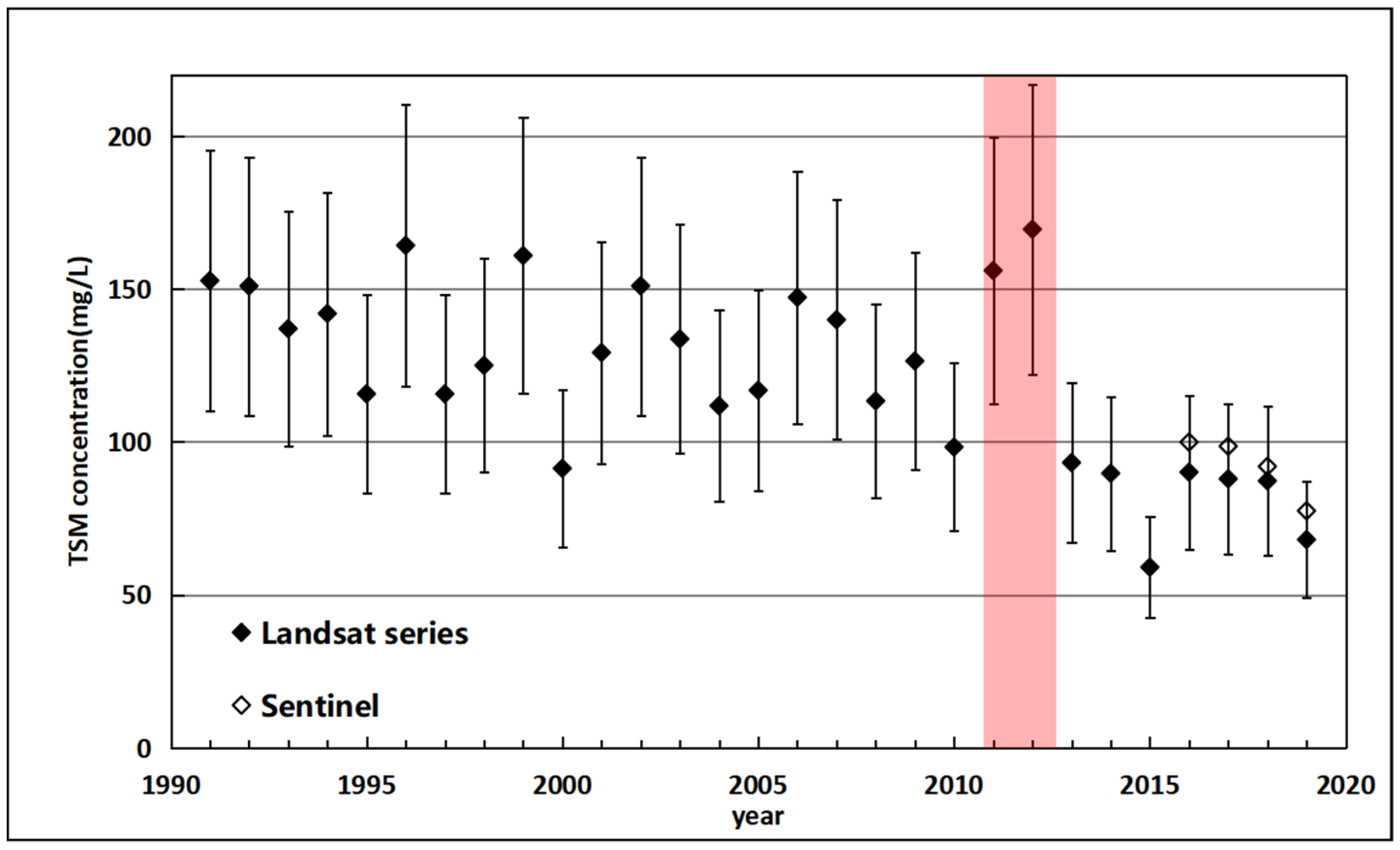
Figure 7 shows the changes in the mean CTSM in the Padma River in the period 1991–2019. During this period, the maximum and minimum CTSM values (194.56 ± 54 and 58.97 ± 16 mg/L, respectively) occurred in 2011 and 2015, respectively. Overall, CTSM displayed a downward trend in this period.
Especially, the strongest global La Niña event in the past six decades occurred in 2011 and 2012. In April of 2011, intense cyclones struck Bangladesh and brought heavy rainfall. In July of 2011, continuous heavy precipitation triggered floods and forced more than 10,000 people to evacuate. The flood caused by La Niña lasted until the summer of 2012. The floods caused a large amount of SM from terrestrial sources to rush into the Padma River, resulting in an abnormally elevated level of turbidity and an abnormally high mean CTSM in 2011 and 2012. At the end of 2012, the impact caused by La Niña weakened, and the CTSM level returned to the normal trend in 2013.
3.5. Changes in FTSM in the Padma River
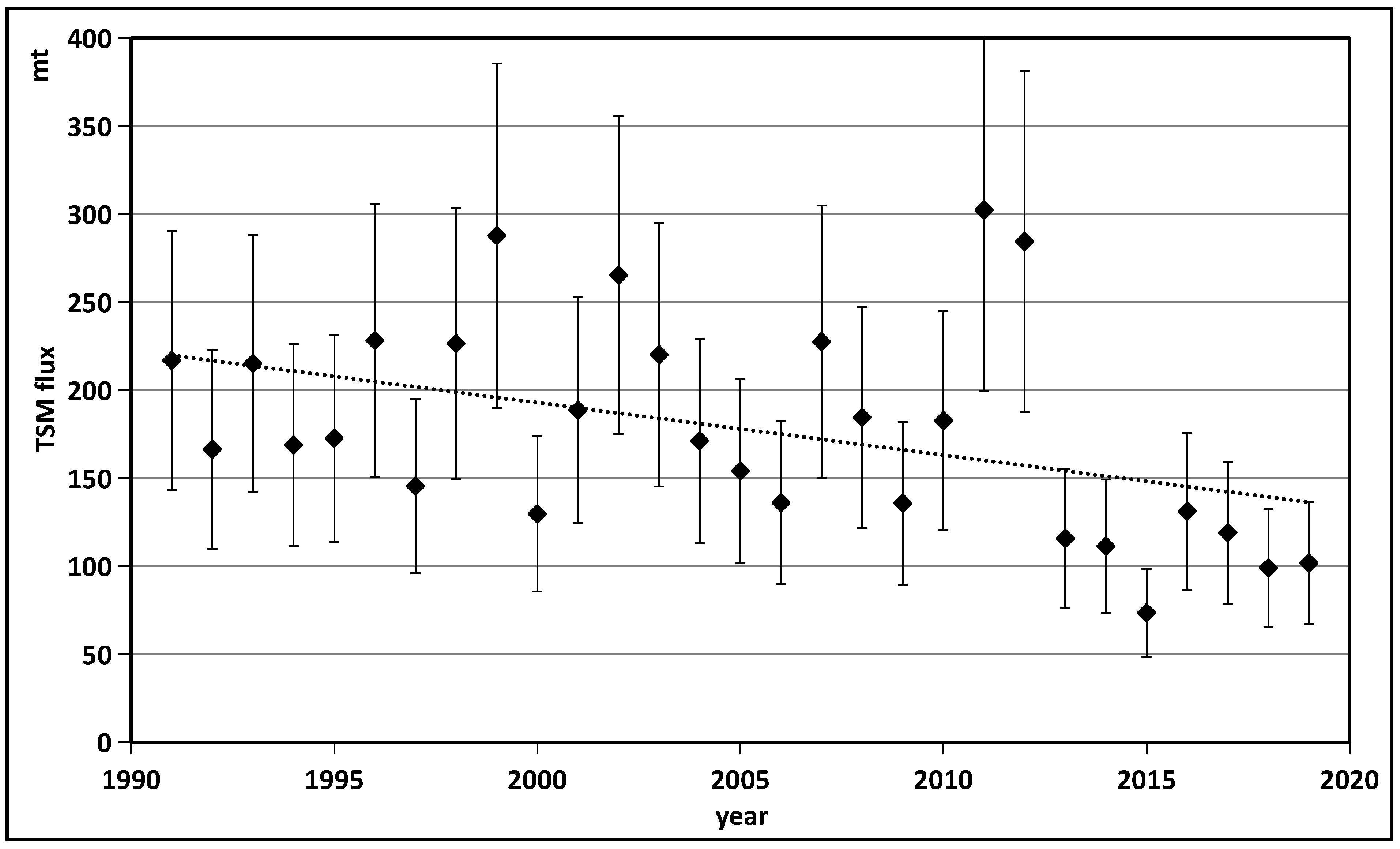
Due to the high flow rate and large discharge in the Padma River, we can approximately consider that the TSM in the Padma River was sufficiently mixed. In addition, the non-tidal reaches were selected in this study for analysis, and, therefore, the tidal effects do not need to be considered. Then, we can approximately consider that the TSM was uniformly distributed in the Padma River. The monthly mean FTSM was calculated through the multiplication of the arithmetic mean CTSM at the selected section (23°10′44″ N) estimated from the Landsat data by the arithmetic mean discharge at the selected section. On this basis, subsequent calculations were performed. Figure 8 shows the changes in FTSM in the Padma River in the period 1991–2019. The maximum and minimum FTSM values (318 ± 62 and 73 ± 29 mt, respectively) occurred in 2011 and 2015, respectively. Due to the impact of the 1998 flood, the discharge and CTSM were at a high level, so the FTSM increased significantly and returned to the normal level in 2000. At the same time, the low flow caused by the drought in 2006 also continued to reduce FTSM and restored in the next year. In 2011, due to the flood disaster caused by La Niña, the discharge and CTSM in Padma River increased significantly, resulting in a significant increase in FTSM level. In 2012, the impact of La Niña continued. Although the discharge decreased, it remained at a high level. At the same time, the erosion of flood on land did not reduce CTSM, so FTSM was still at a high level. In 2013, the flood disaster was over, and CTSM returned to normal level; FTSM also decreased. The time-series data for the changes in FTSM were analyzed using the M–K test. The Z value and its rate of change were obtained (Z = −2.6073, slope = −33.27 × 10⁵, p < 0.01). In the past 30 years, FTSM in the Padma River showed a relatively significant downward trend and, on average, decreased by 3.3 mt each year. The result passed the significance test at a confidence level of 0.01.
3.6. Changes of NDVI in the Padma River
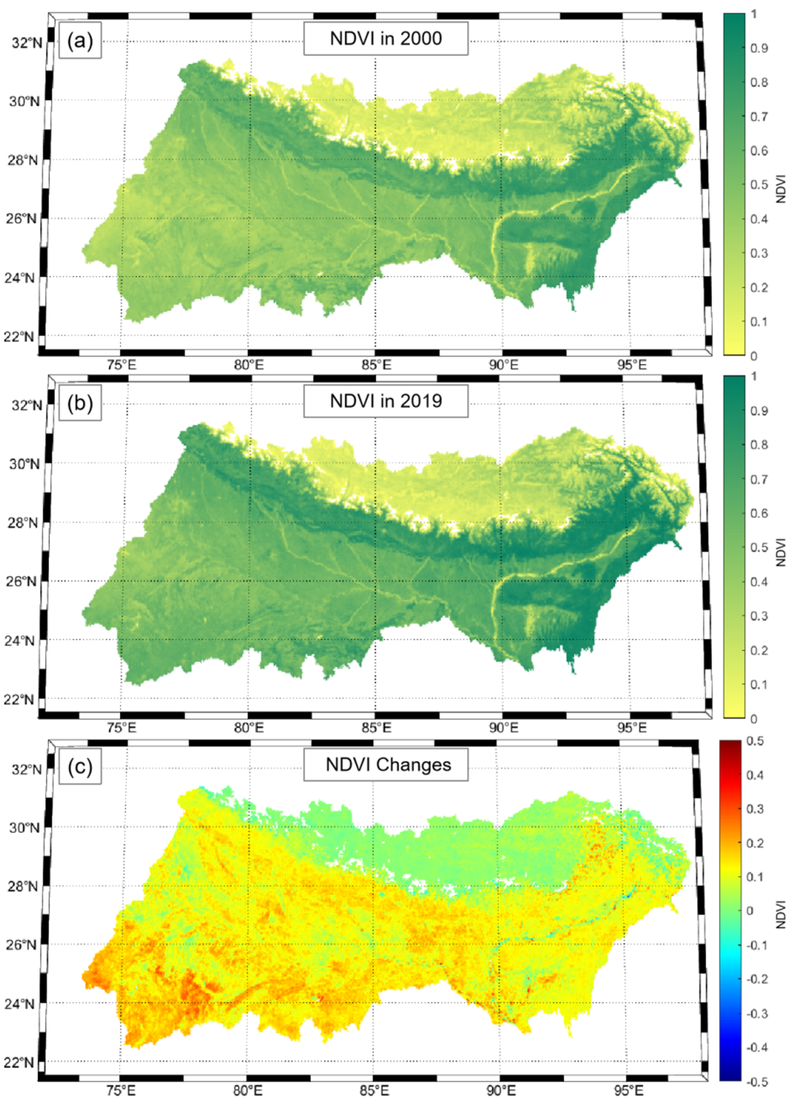
The NDVI for the Padma River Basin was calculated based on the Moderate Resolution Imaging Spectroradiometer (MODIS) global monthly mean NDVI products. The resolution of MODIS NDVI product is 1 km, and the selected coverage covers the whole Padma River Basin. The monthly mean NDVI images for the period 2000–2019 were selected. On the other hand, NDVI along the Padma river is calculated from Landsat images. As shown in Figure 9 and Figure 10, overall, the NDVI for the Padma River Basin displayed an upward trend, suggesting a notable increase in the vegetation coverage along the banks of the Padma River. This suggests that the significant increase in the vegetation coverage in the basin of the Padma River increased the water and soil retention capacity of the land, reduced the extent of soil erosion, and, to a certain extent, reduced the discharge of SM from terrestrial sources, thereby making some contribution to the decrease in the content of TSM in the Padma River.
4. Discussion
4.1. Natural Factors Affecting the Changes in the TSM in the Padma River
Changes in FTSM depend on changes in the discharge and CTSM. The discharge in the Padma River depends primarily on natural factors such as the precipitation and groundwater resources within the river basin and water sources (e.g., freshwater released from the melting of ice on the Tibetan Plateau). The time-series data for the discharge in the Padma River were analyzed using the M–K test. The Z value and its rate of change were obtained (Z = 0.5730, slope = 1.4077 × 10⁸, p > 0.5). The results showed that the discharge itself displayed no notable trend in the past 30 years. In addition, the correlation between the interannual changes in the discharge and FTSM was analyzed. According to the results shown in Figure 11, there was little significant correlation between the changes in the discharge and FTSM (R = 0.44, p < 0.05). Hence, the changes in the discharge might have had a limited impact on FTSM.
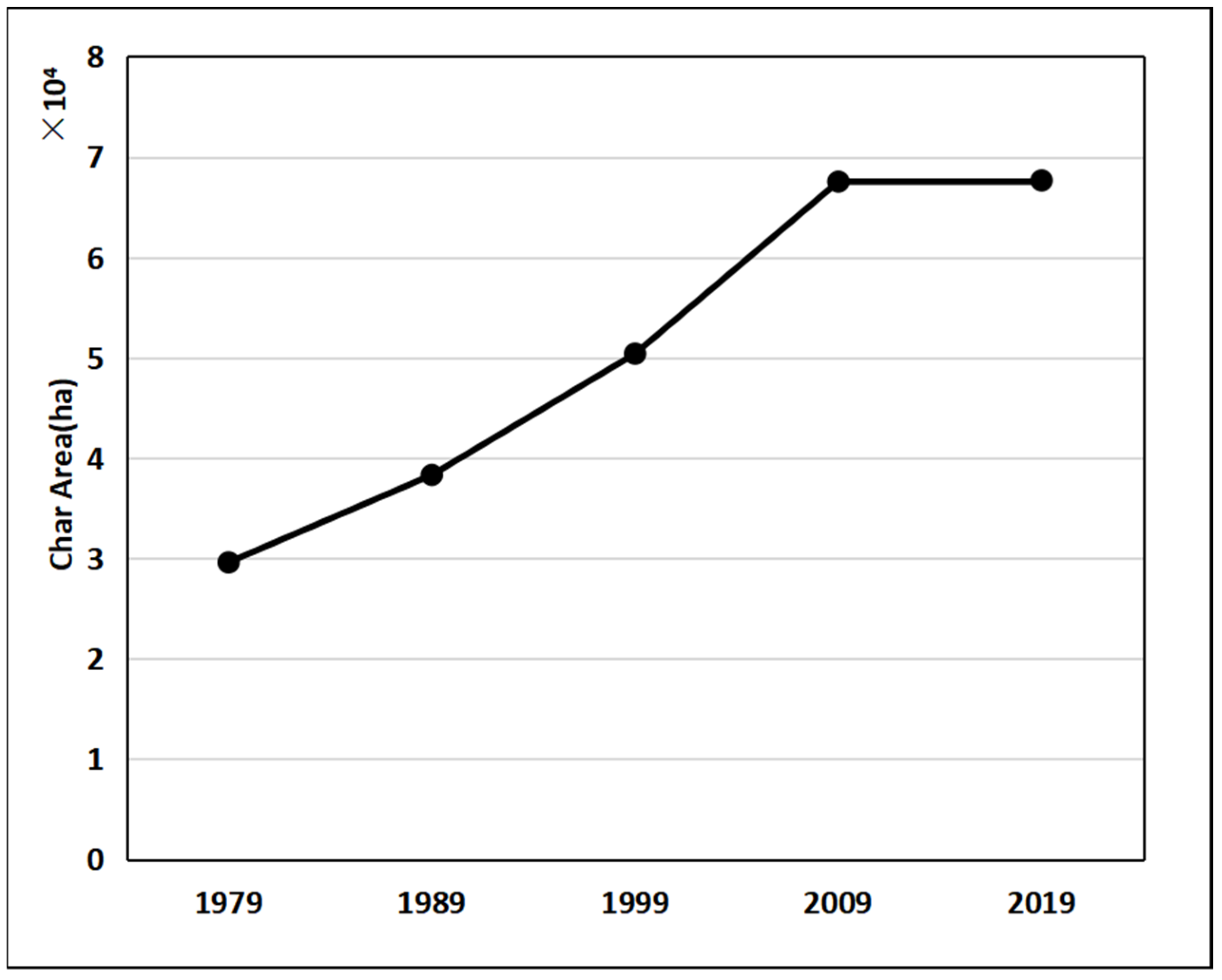
At the same time, the discharge may affect the degree of bank erosion of Padma river. Bank erosion is part of the river system’s natural disruption [38]. The erosion of Padma River is highly irregular [39]. Anupom Halder et al. (2021) studied the change of Padma river bank in the past 40 years by using RS and GIS techniques. The results showed a linear relationship between the erosion and discharge (R2 = 0.9989) [40]. From 1989 to 1999, char land of the Padma River continuously increased (see Figure 12). The island bars were most vulnerable during flooding. Combined with the change analysis of CTSM, it can be seen that char land in Padma River is in a continuous growth state before 2010, and CTSM is also at a stable high concentration level. Char land in Padma stops growing from 2010 to 2019, and CTSM begins to gradually decrease. Unstable char land bar is a major source of TSM, and the area of unstable riparian lines determines the change of CTSM. Therefore, during the study period, although the discharge itself has not changed significantly, the bank erosion of Padma River caused by large discharge and the change of fragile char land area caused by the change of bank line indirectly affect the change of CTSM of Padma River, thus affecting the transportation of FTSM.
4.2. Human Factors Affecting Changes in the TSM in the Padma River
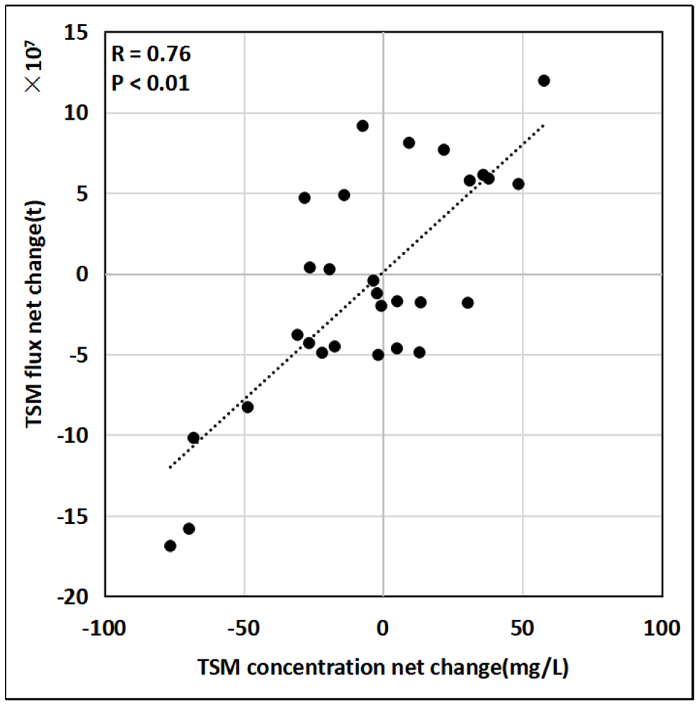
While neglecting the changes in the discharge, we performed a correlation analysis on the annual mean changes in CTSM and FTSM (see Figure 13). A significant correlation (R = 0.76, p < 0.01) was found between the changes in CTSM and FTSM, suggesting that the changes in FTSM in the Padma River depended heavily on the changes in CTSM.
In the Padma River Basin, the changes in CTSM were primarily a result of the changes in the discharge of TSM from terrestrial sources, including the discharge due to soil erosion [41]. As no large reservoirs were constructed in the Ganges–Brahmaputra river system, the impact of water conservancy facilities on FTSM can be excluded. In addition, relatively large discharges may lead to soil erosion and have a greater impact on CTSM. This is particularly true for the Padma River—a river with highly unstable shorelines. The Padma River is relatively wide, with severe bank erosion near Harirampur in the district of Manikganj on its left bank and Naria Upazila in the district of Shariatpur on its right bank. Erosion on the left and right banks of the Padma River occurs at annual rates of 4.82 and 8.19 km2, respectively [42].
Substitution of FTSM series into the M–K abrupt-change test equation yielded UFk and UBk values, as shown in Figure 14. The point of intersection between the UFk and UBk curves correspond to the abrupt-change point of the time series. The abrupt change occurred in 2014. The UFk value fluctuates near 0 before the point of intersection and remains within the a = 0.05 straight line, suggesting that before 2014, the Padma River was relatively stable and its FTSM exhibited no notable trend of change. An abrupt change occurred in 2014, when FTSM began to decrease. This is because, around 2014, the government of Bangladesh began to implement a series of environmental protection measures, adopted a sustainable development strategy, and participated in the Blue Economic Zone Cooperation in the Bay of Bengal [43]. In addition, the government of Bangladesh and non-governmental organizations vigorously carried out afforestation projects along the coast, resulting in a significant increase in the green land area. Vegetation planting, to a certain extent, reduced soil erosion in the coastal zones, thereby reducing the content of TSM [44]. To validate this hypothesis, the NDVI was analyzed.
4.3. Effects of the NDVI on the Changes in CTSM
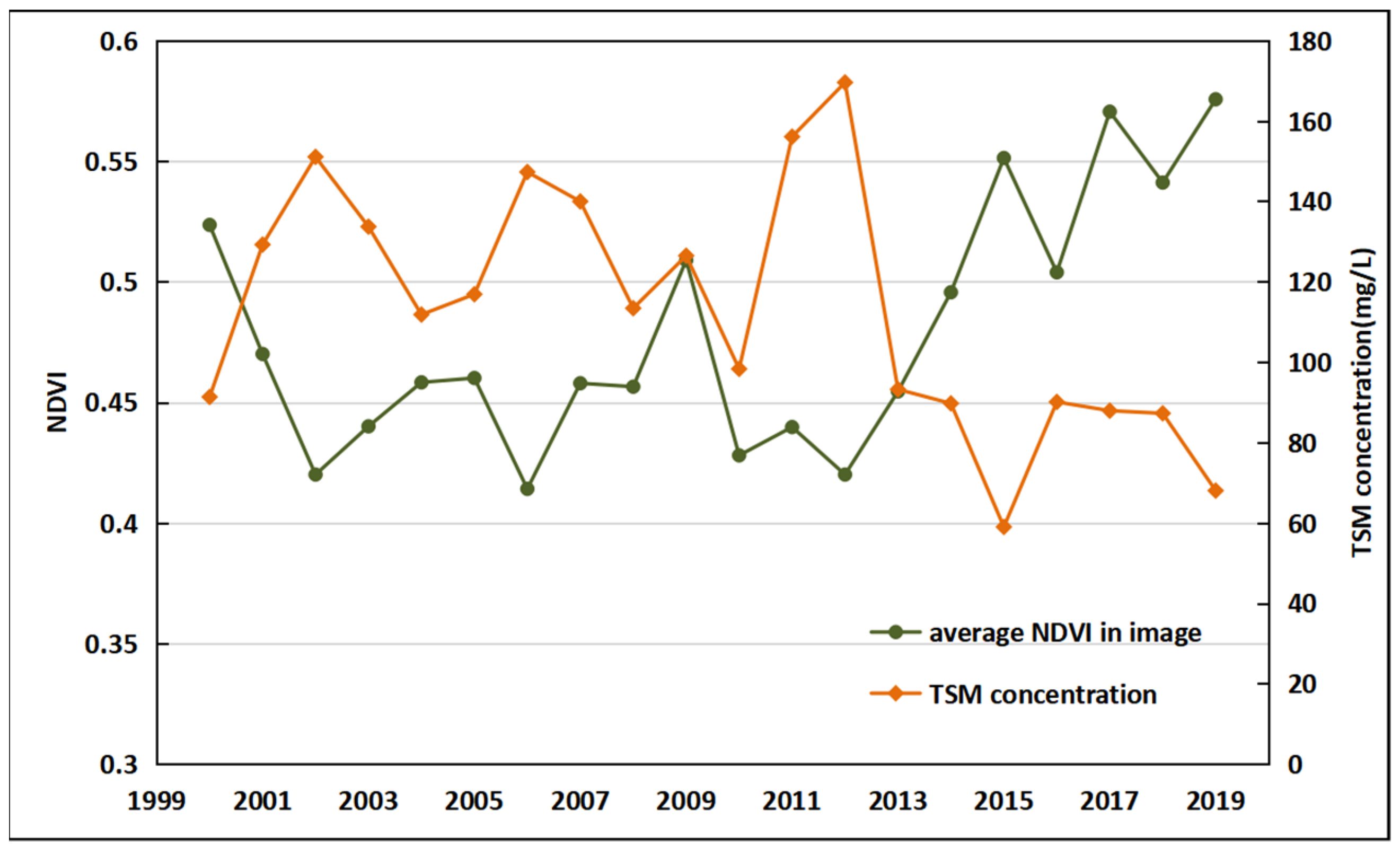
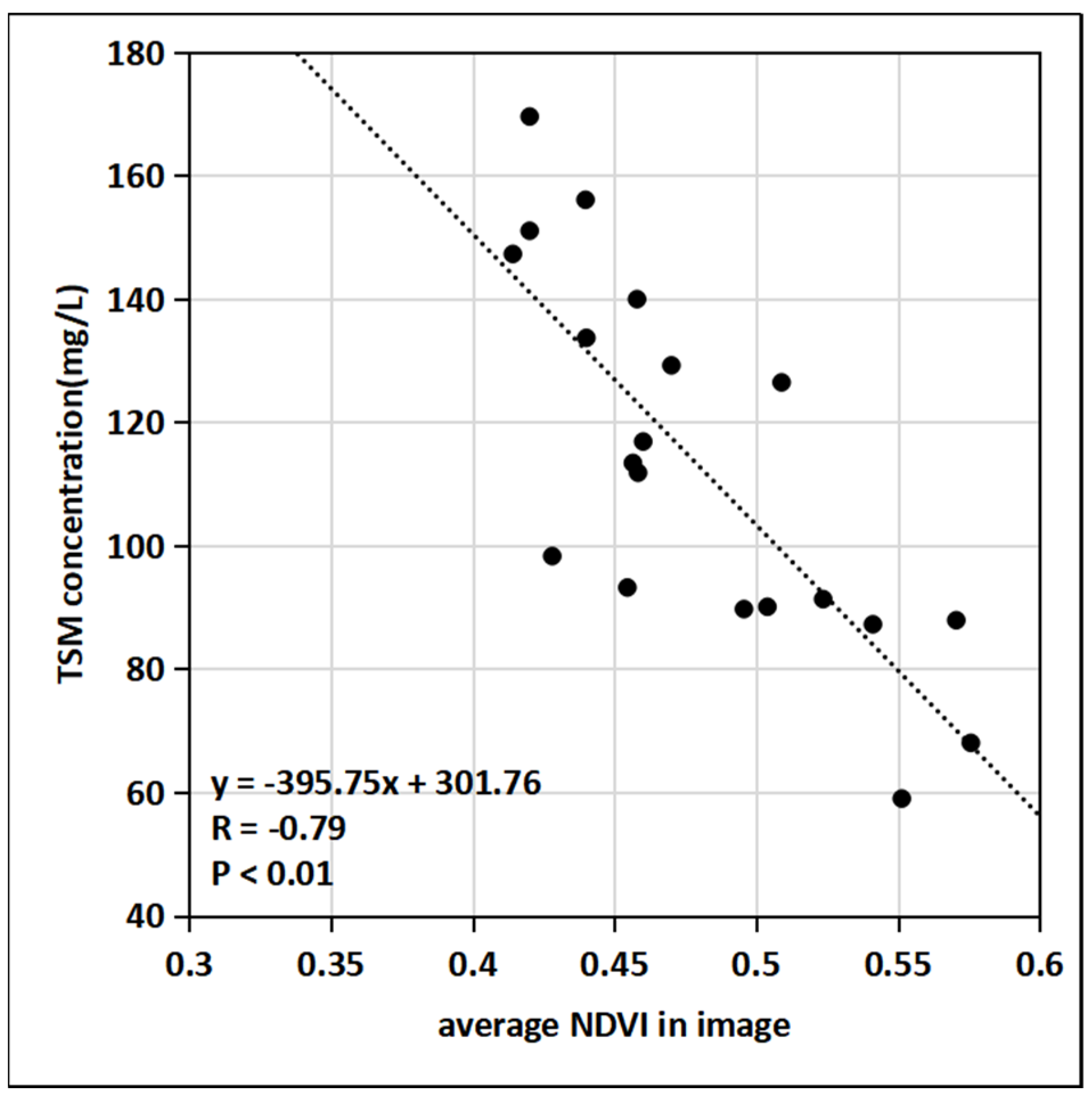
Mithun Kumar et al. (2021), in their monitoring and mapping of forest, cover changes in eastern Sundarban based on satellite remote sensing technology using the maximum likelihood classification approach [45]. The classification map shows that, from 1989 to 2014, the vegetation coverage in the study area decreased by 2.66%, while, from 2014 to 2019, the vegetation coverage increased by 2.22%. Water body and mudfat, low laying area, as well as intertidal zone have been increased with the decrease in vegetation cover. Using Landsat series satellite images separated by water and land, the NDVI mean of land in the image frame is calculated to obtain the change of average NDVI. The trend of the average NDVI in image was opposite to that of CTSM (correlation coefficient R = −0.79, p < 0.01) (see Figure 15), indicating a significantly negative correlation between the NDVI and CTSM. The results show that, from 2000 to 2019, under the background of the overall NDVI value rising in the basin, the NDVI level along the Padma River also shows an upward trend. At the same time, the downward trend before 2014 and the upward trend after 2014 can also be clearly seen. The research area of this study overlaps with that of Mithun et al. (2021) To a certain extent. Therefore, the similar conclusions of the two can also support the results of this study. It should be noted that the vegetation coverage is not completely related to the NDVI index, because in the study range, more vegetation in Padma River basin is transformed into water rather than bare land due to land erosion. At the same time, as mentioned above, in the last decade, due to environmental protection policies and policies to encourage planting, the level of NDVI has increased and the land retention has improved. The improvement of land conservation also slows down the generation of fragile bar lines, so it also slows down the growth of char land area. Thus, the land-based emission of TSM and CTSM in Padma River are reduced. In conclusion, the vegetation cover level and NDVI of the Padma River Basin, especially the coastal land area, will affect the land conservation capacity, thus indirectly affecting the FTSM transport of the Padma River.
5. Conclusions
In this study, CTSM in the Padma River Basin was estimated from the Landsat-8 OLI/TIRS and Landsat-5 TM L1 reflectance products for the period 1991–2019. In addition, the causes of the changes in CTSM were analyzed based on the discharge, precipitation, and NDVI data for the same time period. The main conclusions of this study can be summarized as follows:
(1) The CTSM values in the Padma River were high in areas near the banks and in the downstream region and low in areas away from the banks and in the upstream region. The waters with relatively high CTSM values were distributed in the downstream region near the mouth of the river. Across each year, CTSM was the lowest in winter and spring and the highest in summer and fall.
(2) In the period 1991–2019, the maximum and minimum mean FTSM values in the Padma River (318 ± 62 and 73 ± 29 mt, respectively) occurred in 2011 and 2015, respectively. Abnormally high FTSM values occurred in the year with a strong La Niña event. Overall, FTSM displayed a downward trend and decreased at an annual average rate of 3.3 mt.
(3) The FTSM values in the Padma River depended collectively on the discharge and CTSM at the mouth. Compared with natural factors (e.g., discharge) (R = 0.44, p < 0.05), the changes in CTSM contributed more significantly to the changes in FTSM in the Padma River (R = 0.76, p < 0.01). A significantly negative correlation was found between the NDVI and CTSM (R = −0.79, p < 0.01), suggesting that the increase in the NDVI within the Ganges–Brahmaputra River Basin and the coastal bar line in the last decades led to a decrease in the discharge of TSM from terrestrial sources and CTSM, and that changes in human factors (e.g., vegetation changes) negatively contributed to FTSM in the Padma River. Hence, human activities were the dominant factor causing the changes in FTSM in the Padma River (Ganges–Brahmaputra River system).
This study ensured the accuracy of atmospheric correction of satellite data and the accuracy of various algorithms. However, due to the climatic characteristics of the geographical location of the study area, it is difficult to obtain cloudless and high-quality remote sensing images, so the sufficiency of the amount of remote sensing data cannot be guaranteed. There may not be data available for the entire quarter in summer and autumn in some years. In this case, after calculating the TSM concentration of the seasons with data, we use the following method to make up for the gap in the cloudy season data: Take the multi-year arithmetic average of all TSM data in each season to obtain the CTSM of the four seasons during the 30 years. Then the climatic distribution of each grid point is calculated, and the ratio of the four seasonal climatic CTSM at each grid point is calculated. On this basis, the CTSM of the missing season is calculated based on this ratio. Due to the numerical averaging of the climatic data, although the absolute value of the data may not be so accurate, it should be of good reference value when estimating the trend of the FTSM changes. Because there are few hydrological data in the study area, and because they are difficult to obtain, this study can provide ideas for hydrological research in similar areas.
Author Contributions
Conceptualization, X.H. and D.W.; methodology, Z.Z.; software, validation, Z.Z.; formal analysis, Z.Z. and F.G.; resources, F.G. and D.W.; writing—original draft preparation, Z.Z.; writing—review and editing, D.W., X.H. and Y.B.; supervision, project administration and funding acquisition, D.W. All authors have read and agreed to the published version of the manuscript.
Funding
This research was funded by the National Key R&D Program of China under Grant No. 2018YFB0505005 and 2017YFC1405300, the Key Research and Development Plan of Zhejiang Province under contract No. 2017C03037, the National Natural Science Foundation of China under contract No. 41476157, and the Marine Science and Technology Cooperation Project between Maritime Silk Route and island countries based on marine sustainability.
Acknowledgments
The authors would like to thank the USGS for excellent Landsat and Sentinel data. We also thank the satellite ground station and the satellite data processing and sharing center of SOED/SIO for help with the data processing. Our deepest gratitude goes to the editors and reviewers for their careful work and thoughtful suggestions.
Conflicts of Interest
The authors declare no conflict of interest.
References
- Ouillon, S.; Douillet, P.; Andréfouët, S. Coupling satellite data with in situ measurements and numerical modeling to study fine suspended-sediment transport: A study for the lagoon of New Caledonia. Coral Reefs 2004, 23, 109–122. [Google Scholar]
- Chacko, N.; Jayaram, C. Variability of total suspended matter in the northern coastal Bay of Bengal as observed from satellite data. J. Indian Soc. Remote Sens. 2017, 45, 1077–1083. [Google Scholar] [CrossRef]
- Wilber, D.H.; Clarke, D.G. Biological effects of suspended sediments: A review of suspended sediment impacts on fish and shellfish with relation to dredging activities in estuaries. N. Am. J. Fish. Manag. 2001, 21, 855–875. [Google Scholar] [CrossRef]
- Cyrus, D.P.; Blaber, S.J.M. The influence of turbidity on juvenile marine fishes in estuaries. Part 1. Field studies at Lake St. Lucia on the southeastern coast of Africa. J. Exp. Mar. Biol. Ecol. 1987, 109, 53–70. [Google Scholar] [CrossRef]
- Cyrus, D.P.; Blaber, S.J.M. The influence of turbidity on juvenile marine fishes in estuaries. Part 2. Laboratory studies, comparisons with field data and conclusions. J. Exp. Mar. Biol. Ecol. 1987, 109, 71–91. [Google Scholar] [CrossRef]
- Li, L.; Ni, J.; Chang, F.; Yue, Y.; Frolova, N.; Magritsky, D.; Borthwick, A.G.L.; Ciais, P.; Wang, Y.; Zheng, C.; et al. Global trends in water and sediment fluxes of the world’s large rivers. Sci. Bull. 2020, 65, 62–69. [Google Scholar] [CrossRef] [Green Version]
- Milliman, J.D.; Mei-e, R. River flux to the sea: Impact of human intervention on river systems and adjacent coastal areas. In Climate Change; CRC Press: Boca Raton, FL, USA, 2021; pp. 57–83. [Google Scholar]
- Li, T.; Wang, S.; Liu, Y.; Fu, B.; Zhao, W. Driving forces and their contribution to the recent decrease in sediment flux to ocean of major rivers in China. Sci. Total Environ. 2018, 634, 534–541. [Google Scholar] [CrossRef] [PubMed]
- Darby, S.E.; Hackney, C.R.; Leyland, J.; Kummu, M.; Lauri, H.; Parsons, D.R. Fluvial sediment supply to a mega-delta reduced by shifting tropical-cyclone activity. Nature 2016, 539, 276–279. [Google Scholar] [CrossRef] [Green Version]
- Portenga, E.W.; Bierman, P.R.; Trodick Jr, C.D.; Greene, S.E.; DeJong, B.D.; Rood, D.H.; Pavich, M.J. Erosion rates and sediment flux within the Potomac River basin quantified over millennial timescales using beryllium isotopes. Bulletin 2019, 131, 1295–1311. [Google Scholar] [CrossRef]
- Strick, R.J.; Ashworth, P.J.; Smith, G.H.S.; Nicholas, A.P.; Best, J.L.; Lane, S.N.; Parsons, D.R.; Simpson, C.J.; Unsworth, C.A.; Dale, J. Quantification of bedform dynamics and bedload sediment flux in sandy braided rivers from airborne and satellite imagery. Earth Surf. Process. Landf. 2019, 44, 953–972. [Google Scholar] [CrossRef]
- Rahman, M.M.; Goel, N.K.; Arya, D.S. Development of the jamuneswari flood forecasting system: Case study in bangladesh. J. Hydrol. Eng. 2012, 17, 1123–1140. [Google Scholar] [CrossRef]
- Gallay, M.; Martinez, J.M.; Mora, A.; Castellano, B.; Yépez, S.; Cochonneau, G.; Laraque, A. Assessing Orinoco river sediment discharge trend using MODIS satellite images. J. S. Am. Earth Sci. 2019, 91, 320–331. [Google Scholar] [CrossRef]
- Immerzeel, W.W.; van Beek, L.P.H.; Bierkens, M.F.P. Climate change will affect the Asian water towers. Science 2010, 328, 1382–1385. [Google Scholar] [CrossRef]
- Khan, M.Z.H.; Hasan, M.R.; Khan, Z.H.; Aktar, S.; Fatema, K. Distribution of heavy metals in surface sediments of the Bay of Bengal coast. J. Toxicol. 2017, 2017, 9235764. [Google Scholar] [CrossRef] [PubMed]
- Sarin, M.M.; Krishnaswami, S.; Dilli, K.; Somayajulu, B.L.K.; Moore, W.S. Major ion chemistry of the Ganga–Brahmaputra river system: Weathering processes and fluxes to the Bay of Bengal. Geochim. Cosmochim. Acta 1989, 53, 997–1009. [Google Scholar] [CrossRef]
- Mitra, A.; Gangopadhyay, A.; Dube, A.; Schmidt, A.; Banerjee, K. Observed changes in water mass properties in the Indian Sundarbans (Northwestern Bay of Bengal) during 1980–2007. Curr. Sci. 2009, 97, 1445–1452. [Google Scholar]
- Jutla, A.S.; Akanda, A.S.; Islam, S. Satellite remote sensing of space-time plankton variability in the Bay of Bengal: Connections to cholera outbreaks. Remote Sens. Environ. 2012, 123, 196–206. [Google Scholar] [CrossRef] [Green Version]
- Sridhar, P.N.; Ali, M.M.; Vethamony, P.; Babu, M.T.; Ramana, I.V.; Jayakumar, S. Seasonal occurrence of unique sediment plume in the Bay of Bengal. EOS Trans. 2008, 89, 22–23. [Google Scholar] [CrossRef]
- Sasamal, S.K.; Panigrahy, R.C.; Misra, S. Asterionella blooms in the northwestern Bay of Bengal during 2004. Int. J. Remote Sens. 2005, 26, 3853–3858. [Google Scholar] [CrossRef]
- Milliman, J.D.; Meade, R.H. World-wide delivery of river sediment to the oceans. J. Geol. 1983, 91, 1–21. [Google Scholar] [CrossRef]
- Milliman, J.D.; Syvitski, J.P.M. Geomorphic/tectonic control of sediment discharge to the ocean: The importance of small mountainous rivers. J. Geol. 1992, 100, 525–544. [Google Scholar] [CrossRef]
- Burton, J.D. River inputs into ocean systems: Status and recommendations for research. Final report of SCOR Working Group 46. In UNESCO Technical Papers in Marine Science; No. 55; UNESCO: Paris, France, 1988; p. 25. [Google Scholar]
- Aziz, A.; Paul, A.R. Bangladesh Sundarbans: Present status of the environment and biota. Diversity 2015, 7, 242–269. [Google Scholar] [CrossRef]
- The Daily Star. Over 66,000 Hectares Lost to Padma Since 1967: NASA Report; The Daily Star: Dhaka, Bangladesh, 2018. [Google Scholar]
- Alfieri, L.; Burek, P.; Dutra, E.; Krzeminski, B.; Muraro, D.; Thielen, J. GloFAS—Global ensemble streamflow forecasting and flood early warning. Hydrol. Earth Syst. Sci. 2013, 17, 1161–1175. [Google Scholar] [CrossRef] [Green Version]
- Adler, R.; Wang, J.J.; Sapiano, M.; Huffman, G.; Chiu, L.; Xie, P.P.; NOAA CDR Program. Global Precipitation Climatology Project (GPCP) Climate Data Record (CDR), Version 2.3 (Monthly); National Centers for Environmental Information: Washington, DC, USA, 2016. [CrossRef]
- Hossain, S.; Cloke, H.L.; Ficchì, A.; Turner, A.G.; Stephens, E. Hydrometeorological drivers of the 2017 flood in the brahmaputra basin in bangladesh. Hydrol. Earth Syst. Sci. Discuss. 2019, 1–33. [Google Scholar] [CrossRef] [Green Version]
- Schroeder, T.A.; Cohen, W.B.; Song, C.; Canty, M.J.; Yang, Z. Radiometric correction of multi-temporal Landsat data for characterization of early successional forest patterns in western Oregon. Remote Sens. Environ. 2006, 103, 16–26. [Google Scholar] [CrossRef]
- Felde, G.W.; Anderson, G.P.; Cooley, T.W.; Matthew, M.W.; Adler-Golden, S.M.; Berk, A.; Lee, J. Analysis of Hyperion Data with the FLAASH Atmospheric Correction Algorithm. In Proceedings of the 2003 IEEE International Geoscience and Remote Sensing Symposium, Toulouse, France, 21–25 July 2003. [Google Scholar]
- Liu, D.; Bai, Y.; He, X.; Pan, D.; Chen, C.-T.A.; Li, T.; Xu, Y.; Gong, C.; Zhang, L. Satellite-derived particulate organic carbon flux in the Changjiang River through different stages of the Three Gorges Dam. Remote Sens. Environ. 2019, 223, 154–165. [Google Scholar] [CrossRef]
- Roy, D.P.; Kovalskyy, V.; Zhang, H.K.; Vermote, E.F.; Yan, L.; Kumar, S.S.; Egorov, A. Characterization of Landsat-7 to Landsat-8 reflective wavelength and normalized difference vegetation index continuity. Remote Sens. Environ. 2016, 185, 57–70. [Google Scholar] [CrossRef] [Green Version]
- Kendall, M.G. Rank correlation methods. Br. J. Psychol. 1990, 25, 86–91. [Google Scholar] [CrossRef]
- Mann, H.B. Nonparametric tests against trend. Econometrica 1945, 13, 245–259. [Google Scholar] [CrossRef]
- Shao, Z.; Cai, J.; Fu, P.; Hu, L.; Liu, T. Deep learning-based fusion of Landsat-8 and Sentinel-2 images for a harmonized surface reflectance product. Remote Sens. Environ. 2019, 235, 111425. [Google Scholar] [CrossRef]
- Zhang, H.K.; Roy, D.P.; Yan, L.; Li, Z.; Huang, H.; Vermote, E.; Skakun, S.; Roger, J.-C. Characterization of Sentinel-2A and Landsat-8 top of atmosphere, surface, and nadir BRDF adjusted reflectance and NDVI differences. Remote Sens. Environ. 2018, 215, 482–494. [Google Scholar] [CrossRef]
- Tucker, C.J. Red and photographic infrared linear combinations for monitoring vegetation. Remote Sens. Environ. 1979, 8, 127–150. [Google Scholar] [CrossRef] [Green Version]
- Mount, J.F.; Florsheim, J.L.; Chin, A. Bank erosion as a desirable attribute of rivers. BioScience 2008, 58, 519–529. [Google Scholar]
- Dewan, A.; Corner, R.; Saleem, A.; Rahman, M.M.; Haider, M.R.; Rahman, M.M.; Sarker, M.H. Assessing channel changes of the ganges-padma river system in bangladesh using landsat and hydrological data. Geomorphology 2017, 276, 257–279. [Google Scholar] [CrossRef]
- Halder, A.; Chowdhury, R.M. Evaluation of the river Padma morphological transition in the central Bangladesh using GIS and remote sensing techniques. Int. J. River Basin Manag. 2021, 1–15. [Google Scholar] [CrossRef]
- Sarker, M.H.; Thorne, C.R. Morphological response of the Brahmaputra–padma–lower Meghna river system to the Assam earthquake of 1950. Braided Rivers Process. Depos. Ecol. Manag. 2006, 21, 289–310. [Google Scholar]
- Rashid, M.B. Channel bar development and bankline migration of the Lower Padma River of Bangladesh. Arab. J. Geosci. 2020, 13, 1–16. [Google Scholar] [CrossRef]
- Hussain, M.G.; Failler, P.; Karim, A.A.; Alam, M.K. Major opportunities of blue economy development in Bangladesh. J. Indian Ocean Reg. 2018, 14, 88–99. [Google Scholar] [CrossRef]
- Zheng, F.-L. Effect of vegetation changes on soil erosion on the Loess Plateau. Pedosphere 2006, 16, 420–427. [Google Scholar] [CrossRef]
- Kumar, M.; Mondal, I.; Pham, Q.B. Monitoring forest landcover changes in the Eastern Sundarban of Bangladesh from 1989 to 2019. Acta Geophys. 2021, 69, 561–577. [Google Scholar] [CrossRef]
Figure 1.
Illustration of the location of the study area. The image on the left-hand side shows a map of the East Asian continent with digital elevation model (DEM) data downloaded from USGS as the background. The blue lines signify six large rivers originating from the Tibetan Plateau. The area within the black outline is the Ganges–Brahmaputra River Basin, while the area within the red box is the study area. The image on the right-hand side is an example of a Landsat 5 TM image of the Padma River (taken on 17 October 1994).

Figure 2.
Location of the section selected for calculating FTSM. The color bar shows the number of effective values of each pixel. The section was selected from the branchless part of the river with a relatively large amount of available data. North of the section are mostly input tributaries, while south of the section are mostly distributories. The contributions of the tributaries were also considered when the flux was calculated.

Figure 3.
Location of the areas in the Landsat and Sentinel images (the image with a red border is the Sentinel image, and the image with a blue border is the Landsat image).
Figure 3.
Location of the areas in the Landsat and Sentinel images (the image with a red border is the Sentinel image, and the image with a blue border is the Landsat image).

Figure 4.
Changes of Padma River discharge and precipitation in the basin during the study period. The figures on the left and right show the average annual discharge and precipitation and the average monthly discharge and precipitation, respectively.
Figure 4.
Changes of Padma River discharge and precipitation in the basin during the study period. The figures on the left and right show the average annual discharge and precipitation and the average monthly discharge and precipitation, respectively.

Figure 5.
Comparison of the NIR-band/blue-band ratios between the Landsat and Sentinel data.

Figure 6.
Distribution of CTSM in the Padma River in: (a) winter, (b) spring, (c) summer, and (d) fall.
Figure 6.
Distribution of CTSM in the Padma River in: (a) winter, (b) spring, (c) summer, and (d) fall.

Figure 7.
Changes in CTSM in the Padma River in the period 1991–2019, and the red area represents the duration of La Niña.
Figure 7.
Changes in CTSM in the Padma River in the period 1991–2019, and the red area represents the duration of La Niña.

Figure 8.
Changes in FTSM in the Padma River in the period 1991–2019. The dotted line is the linear regression of FTSM.
Figure 8.
Changes in FTSM in the Padma River in the period 1991–2019. The dotted line is the linear regression of FTSM.

Figure 9.
Mean NDVI values from MODIS for the Ganges–Brahmaputra River Basin. (a) Mean NDVI value for the river basin in 2000. (b) Mean NDVI value for the river basin in 2019. (c) Changes in the mean NDVI value between 2000 and 2019.
Figure 9.
Mean NDVI values from MODIS for the Ganges–Brahmaputra River Basin. (a) Mean NDVI value for the river basin in 2000. (b) Mean NDVI value for the river basin in 2019. (c) Changes in the mean NDVI value between 2000 and 2019.

Figure 10.
Changes in the average NDVI value for the Landsat image as well as the CTSM at the mouth of the river in the period 2000–2019.
Figure 10.
Changes in the average NDVI value for the Landsat image as well as the CTSM at the mouth of the river in the period 2000–2019.

Figure 11.
Correlation between the changes in the discharge and FTSM in the Padma River.

Figure 12.
Char area change of the Padma River [40].
Figure 12.
Char area change of the Padma River [40].

Figure 13.
Correlation between the changes in CTSM and FTSM in the Padma River.

Figure 14.
M–K abrupt-change test results for FTSM in the Padma River. The blue UFk curve and red UBk curve signify the sequential and reversed time series for FTSM, respectively. The critical values for the significance levels a = 0.05 and 0.01 (U0.05 and U0.01, respectively) are ±1.96 and ±2.32, respectively.

Figure 15.
Correlation between the mean NDVI value for the Landsat image and CTSM at the mouth of the river in the period 2000–2019.
Figure 15.
Correlation between the mean NDVI value for the Landsat image and CTSM at the mouth of the river in the period 2000–2019.


Table 1.
Comparison of the characteristics of the Yangtze and Padma Rivers.
| River | CTSM in the River | Sensitive Bands for TSM | Rainy Season | Average Chlorophyll Concentration at the Estuary | Data Sources |
|---|---|---|---|---|---|
| Yangtze River | 30.5–735.4 mg/L | B4 and B1 | May–October | 3.60 mg/L | Liu et al. (2019) [31] |
| Padma River | 32.2–821.7 mg/L | B4 and B1 | May–October | 5.54 mg/L | Rahman et al. (2016) [12] and Jutla et al. (2012) [18] |
Table 2.
Transformation functions between ETM+ and OLI top-of-atmosphere reflectance sensors developed through ordinary-least-squares (OLS) regression (Roy et al. [32]).
Table 2.
Transformation functions between ETM+ and OLI top-of-atmosphere reflectance sensors developed through ordinary-least-squares (OLS) regression (Roy et al. [32]).
| Band | Sensor Transformation Functions | n | R2 (p Value) | Mean DifferenceOLI—ETM+ (Reflectance) | Mean Relative Difference OLI—ETM+ (%) | Root-Mean-Square Deviation (Reflectance) |
|---|---|---|---|---|---|---|
| Blue (~0.48 μm) | OLI = 0.0173 + 0.8707 ETM+ | 29,697,049 | 0.710 (<0.0001) | 0.0013 | 0.69 | 0.0259 |
| ETM+ = 0.0219 + 0.8155 OLI | ||||||
| Near infrared (~0.85 μm) | OLI = 0.0374 + 0.9281 ETM+ | 29,767,214 | 0.711 (<0.0001) | 0.0194 | 6.45 | 0.0637 |
| ETM+ = 0.0438 + 0.7660 OLI |
Table 3.
Transformation functions between the Sentinel-2 MSI and Landsat-8 OLI developed through OLS regression (Zhang et al. [36]).
Table 3.
Transformation functions between the Sentinel-2 MSI and Landsat-8 OLI developed through OLS regression (Zhang et al. [36]).
| Band | Transformation Function | Sample Size | R2 (p Value) | Mean OLI—MSI Difference | Mean Relative OLI—MSI Difference (%) |
|---|---|---|---|---|---|
| Blue λ (~0.48 μm) | OLI = 0.0003 + 0.9570 MSI MSI = 0.0039 + 0.9383 OLI | 65,347,909 | 0.8980 (<0.0001) | −0.0014 | −4.64 |
| Near infrared λ (~0.85 μm) MSI Band 8A | OLI = 0.0077 + 0.9644 MSI MSI = 0.0147 + 0.9355 OLI | 65,380,148 | 0.9022 (<0.0001) | −0.0003 | −0.22 |
Publisher’s Note: MDPI stays neutral with regard to jurisdictional claims in published maps and institutional affiliations. |
© 2021 by the authors. Licensee MDPI, Basel, Switzerland. This article is an open access article distributed under the terms and conditions of the Creative Commons Attribution (CC BY) license (https://creativecommons.org/licenses/by/4.0/).
Share and Cite
MDPI and ACS Style
Zheng, Z.; Wang, D.; Gong, F.; He, X.; Bai, Y. A Study on the Flux of Total Suspended Matter in the Padma River in Bangladesh Based on Remote-Sensing Data. Water 2021, 13, 2373. https://doi.org/10.3390/w13172373
AMA Style
Zheng Z, Wang D, Gong F, He X, Bai Y. A Study on the Flux of Total Suspended Matter in the Padma River in Bangladesh Based on Remote-Sensing Data. Water. 2021; 13(17):2373. https://doi.org/10.3390/w13172373
Chicago/Turabian StyleZheng, Zhuoqi, Difeng Wang, Fang Gong, Xianqiang He, and Yan Bai. 2021. "A Study on the Flux of Total Suspended Matter in the Padma River in Bangladesh Based on Remote-Sensing Data" Water 13, no. 17: 2373. https://doi.org/10.3390/w13172373
Note that from the first issue of 2016, this journal uses article numbers instead of page numbers. See further details here.