
Impact of Global Warming on Dissolved Oxygen and BOD Assimilative Capacity of the World’s Rivers: Modeling Analysis


1
Department of Civil and Environmental Engineering, Tufts University, Medford, MA 02155, USA
2
Environmental Engineering Research Center (CIIA), Civil and Environmental Engineering Department, Universidad de los Andes, Bogotá 111111, Colombia
3
National Institute of Water and Atmospheric Research (NIWA), P.O. Box 11-115, Hamilton 3251, New Zealand
*
Author to whom correspondence should be addressed.
Water 2021, 13(17), 2408; https://doi.org/10.3390/w13172408
Submission received: 27 May 2021
/
Revised: 16 August 2021
/
Accepted: 26 August 2021
/
Published: 1 September 2021
(This article belongs to the Special Issue Water-Quality Modeling)
Abstract
:For rivers and streams, the impact of rising water temperature on biochemical oxygen demand (BOD) assimilative capacity depends on the interplay of two independent factors: the waterbody’s dissolved oxygen (DO) saturation and its self-purification rate (i.e., the balance between BOD oxidation and reaeration). Although both processes increase with rising water temperatures, oxygen depletion due to BOD oxidation increases faster than reaeration. The net result is that rising temperatures will decrease the ability of the world’s natural waters to assimilate oxygen-demanding wastes beyond the damage due to reduced saturation alone. This effect should be worse for nitrogenous BOD than for carbonaceous BOD because of the former’s higher sensitivity to rising water temperatures. Focusing on streams and rivers, the classic Streeter–Phelps model was used to determine the magnitude of the maximum or “critical” DO deficit that can be calculated analytically as a function of the mixing-point BOD concentration, DO saturation, and the self-purification rate. The results indicate that high-velocity streams will be the most sensitive to rising temperatures. This is significant because such systems typically occur in mountainous regions where they are also subject to lower oxygen saturation due to decreased oxygen partial pressure. Further, they are dominated by salmonids and other cold-water fish that require higher oxygen levels than warm-water species. Due to their high reaeration rates, such systems typically exhibit high self-purification constants and consequently have higher assimilation capacities than slower moving lowland rivers. For slow-moving rivers, the total sustainable mixing-point concentration for CBOD is primarily dictated by saturation reductions. For faster flowing streams, the sensitivity of the total sustainable load is more equally dependent on temperature-induced reductions in both saturation and self-purification.
1. Introduction
Physicians monitor vital signs, such as body temperature, heart rate, and blood pressure, as baseline indicators of a patient’s health status. Because of its relevance to wastewater assimilation, aquatic life, taste and odor problems, and sediment–water interactions, dissolved oxygen (DO) concentration has been, and still is, the best “vital sign” of a waterbody’s ecosystem health. Hence, assessing how climate change might affect the oxygen content of the world’s surface waters is a critical question related to future water quality in a warming climate.
In the present paper, the classic Streeter–Phelps model [1] and the concept of sustainable assimilative capacity are used to address this question broadly and generally. After examining the direct effect of rising water temperatures on oxygen saturation, the analysis is extended to evaluate the influence of rising water temperatures on a river’s ability to break down oxygen-depleting pollutants (BOD). In addition to lowering saturation, rising water temperatures will decrease a river’s assimilative capacity by influencing its oxygen metabolism. Specifically, rising temperatures have a greater effect on the biochemical processes that deplete oxygen than on the atmospheric gas transfer that replenishes it.
It should be noted that the analyses were informed by earlier efforts [2,3,4] to use the Streeter–Phelps model to draw broad conclusions related to a river’s BOD assimilative capacity. Because those contributions were made before climate change was universally accepted, the earlier efforts did not explicitly address the issue explored in this paper: how river oxygen levels will be influenced by rising water temperatures due to global warming.
2. Methods and Results
Quantifying a natural water’s capacity to assimilate oxygen-demanding pollutants depends on the interplay of three main factors: (a) the oxygen saturation concentration, (b) the oxygen concentration necessary to protect ecosystem health and designated uses, and (c) the water body’s BOD assimilative capacity as determined by the physical, chemical, and biological processes that reduce and replenish oxygen.
2.1. Oxygen Saturation
If a beaker of gas-free distilled water is opened to the atmosphere, gases such as oxygen cross the air–water interface until an equilibrium is established between the partial pressure of the gas in the atmosphere and its concentration in the water. At this equilibrium, the water is said to be “saturated” with the gas. Waters with concentrations below saturation are said to have a “deficit” whereas those with concentrations above saturation are said to be “supersaturated”. Hence, by defining the oxygen concentration of an unpolluted water, the oxygen saturation concentration represents the baseline of any effort to assess oxygen-based water quality. Of course, certain rivers are naturally below saturation; for example, those draining watersheds with naturally nutrient-rich soils. However, because of the general nature of our analysis, a goal was needed that is independent of any particular river’s natural metabolism. With this in mind, DO saturation provides a universal definition of a pristine aquatic ecosystem.
Dissolved oxygen saturation depends on temperature, salinity, and oxygen partial pressure. These factors influence saturation as described by [5]
where os = dissolved oxygen saturation concentration (mgO2/L), ϕelev = the fractional reduction of freshwater sea-level saturation due to elevation above sea level (dimensionless), ϕS = the fractional reduction of freshwater sea-level saturation due to salinity (dimensionless), and osf = the dissolved oxygen saturation concentration of sea-level freshwater (mgO2/L). The individual effects of temperature, salinity, and elevation are quantified as follows.
Temperature, T (°C): The oxygen saturation of freshwater at sea level is determined by evaluating the exponent of the exponential function of Equation (1) with [5]
where Ta = absolute temperature (K) = T + 273.15.
Salinity, S (ppt): The oxygen saturation of sea water is obtained by multiplying the sea-level freshwater saturation by [5]
Elevation, elev (km): The effect of atmospheric pressure on gas saturation at elevation is based on the standard atmosphere as described by the cubic polynomial [6]
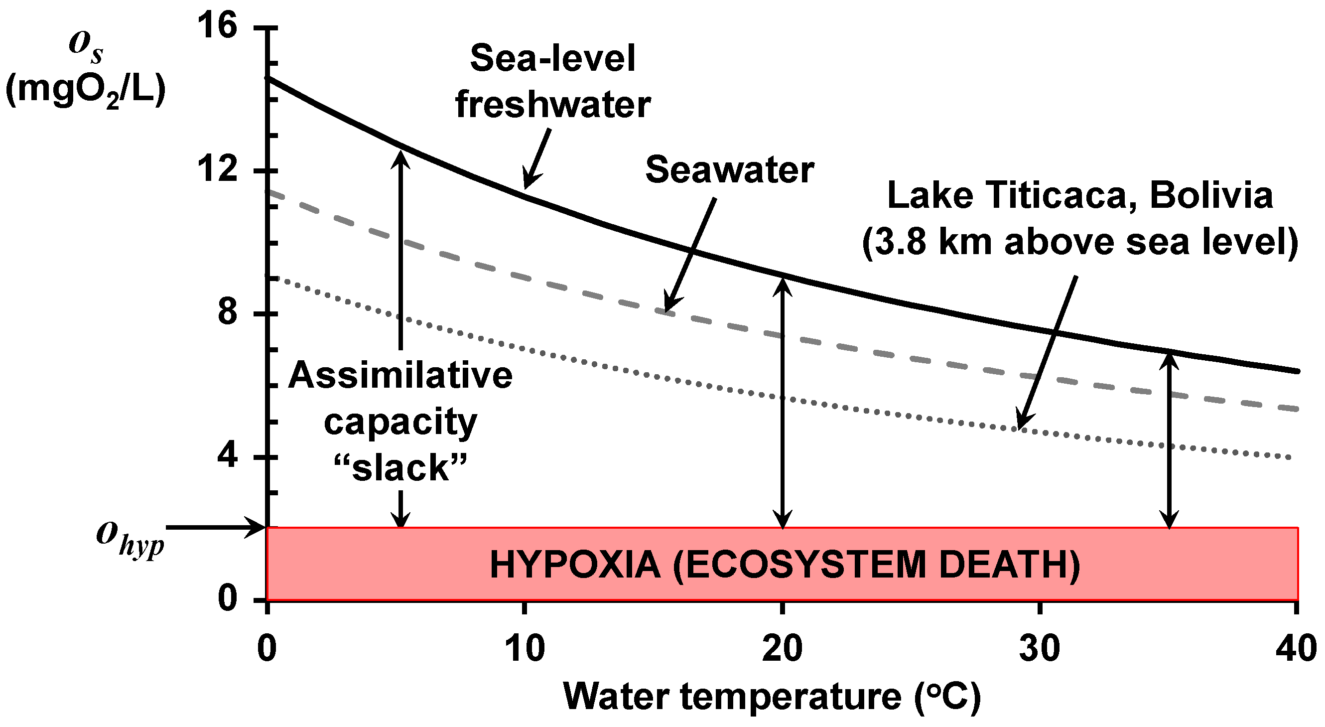
The impact of all three factors is depicted in Figure 1, which shows the relationship of saturation to temperature for three water-body types: sea-level freshwater, seawater, and the world’s highest navigable lake. Rising water temperature lowers the saturation for all three types and is exacerbated by both salinity and elevation above sea level.
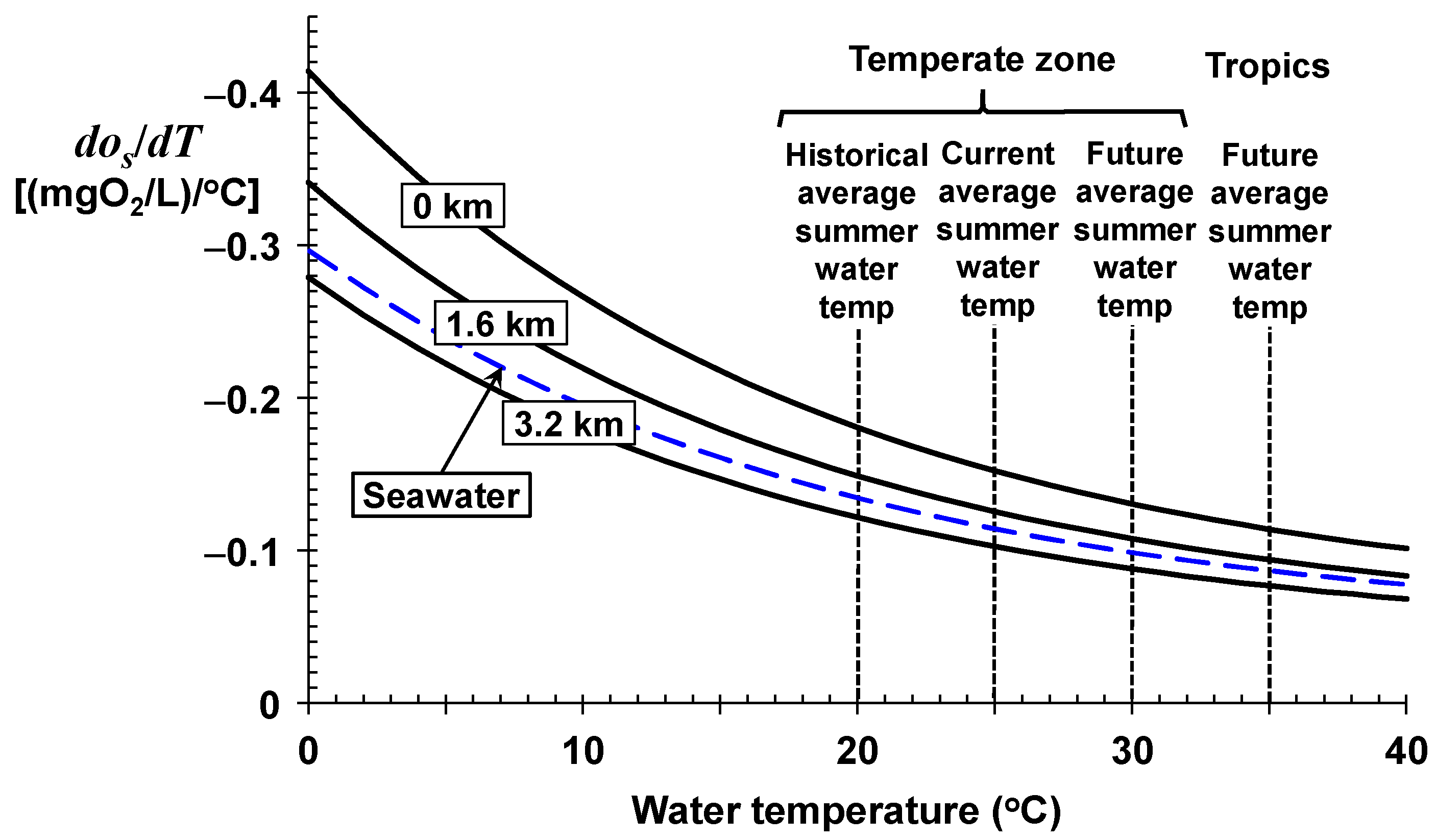
Although the saturation values provide a useful perspective on how oxygen saturation is impacted by temperature, salinity, and elevation, additional insight can be gleaned by computing the rate of change of saturation by differentiating Equation (1) with respect to temperature. Although functions like Equation (1) can sometimes be differentiated analytically, the results are cumbersome and typically provide no insight. Numerical differentiation provides an alternative means to obtain the same results with the centered divided difference [7]
where x = the value of the independent variable, f′(x) = the function’s first derivative with respect to x evaluated at x, and δ = a very small perturbation of x. For the present case, with x = T and f(x) = os(T), the result is dos(T)/dT with units of (mgO2/L)/°C. Thus, the derivative represents a sensitivity factor that quantifies the change in saturation for a unit change in temperature.
As depicted in Figure 2 and listed in Table 1, the sensitivity factors range between a drop of about 0.41 (mgO2/L)/°C for very cold, sea-level freshwaters down to about 0.07 (mgO2/L)/°C for very warm, high-altitude freshwaters. For seawater, the drop ranges from about 0.30 down to about 0.08 (mgO2/L)/°C for very cold and very warm water temperatures, respectively.
These conclusions regarding oxygen saturation are independent of waterbody type, and hence, would apply to all the world’s waters including lakes, estuaries, and marine waters. In the remainder of this paper, the focus will be on rivers. Because most rivers and streams have low salinity, the following analyses concentrate on how temperature and elevation affect the oxygen saturation of fresh waters.
2.2. Oxygen Concentration Standard
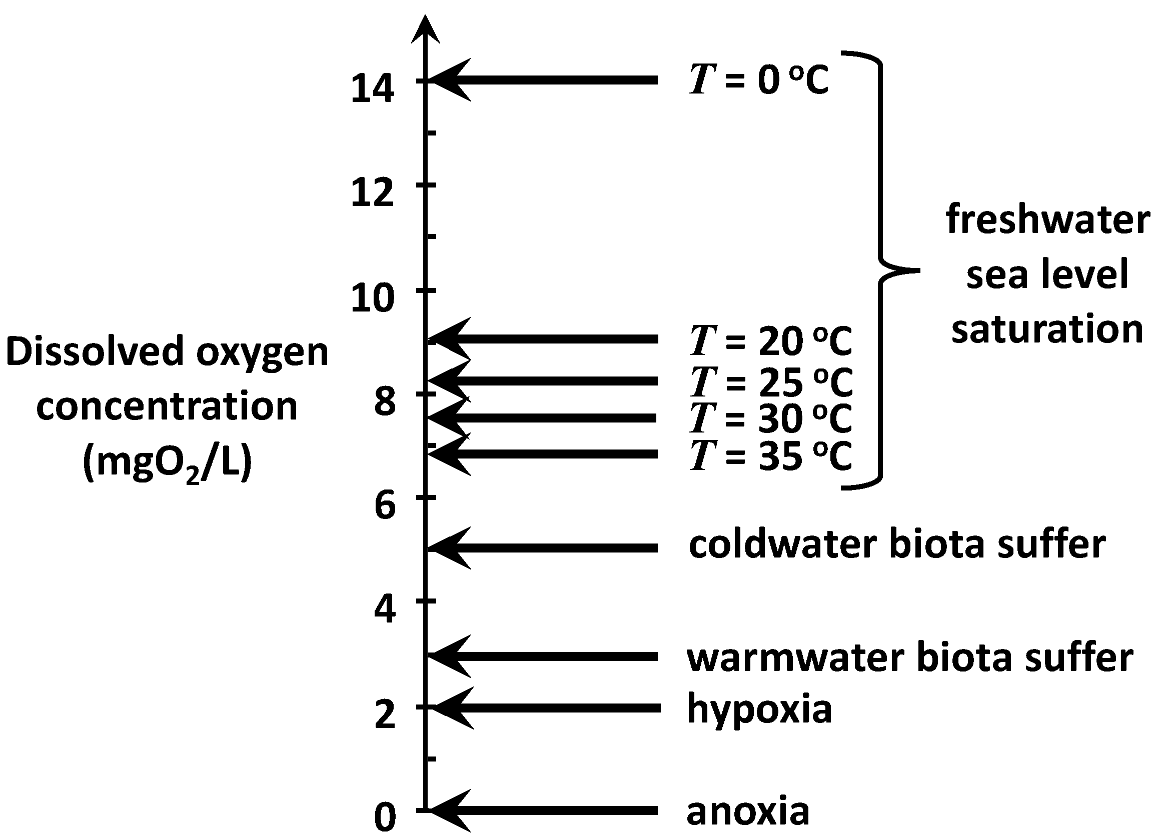
The second factor required to assess oxygen assimilative capacity is the specification of a dissolved oxygen water-quality standard, owq (mgO2/L). This is the oxygen concentration needed to protect ecosystem health and designated uses. Figure 3 is an attempt to generally summarize commonly used target levels to achieve these goals. Freshwater, sea-level saturation concentrations at 5 °C increments between 20 and 35 °C are indicated because this range would encompass the present and future summer temperatures in most of the world’s rivers over the next 50 years.
It should be noted that nutrient-rich waters with high plant photosynthesis can become supersaturated with oxygen, particularly toward dusk. However, these elevated levels typically occur in the warmer months in eutrophic systems and are often short in duration due to algal blooms. Consequently, persistent oxygen levels above 12 mgO2/L are uncommon in critical periods for almost all waterbodies.
The concentration at which biota suffer is roughly in the range of 3–5 mgO2/L but vary somewhat depending on dominant species and life stages of organisms. Hypoxia means “low oxygen” and is usually defined as the level at which oxygen becomes so low that most oxygen-dependent aquatic life is not viable. Anoxia means “no oxygen” and is the point at which a volume of water and its underlying sediments are considered a “dead zone” as far as aerobic organisms are concerned. Along with aerobe death, anoxic systems manifest other undesirable symptoms such as the bottom sediment release of nutrients, toxic compounds, and foul-smelling, noxious gases. Further, anoxia can stress or kill aerobic organisms in the sediments such as macrofauna. This can diminish bioturbation, which is an important process in sediment diagenesis [8].
For the present analysis, an oxygen standard of 2 mgO2/L is assumed to avoid hypoxia, the condition at which a waterbody can no longer support aquatic organisms. This conventional definition is employed recognizing full well that hypoxia can occur in many natural waters at levels above 2 mgO2/L [9]. It is also acknowledged that water-quality standards well above the critical state of hypoxia are typically required to protect oxygen-dependent resources such as sport and commercial fisheries as well as aquaculture. That said, assuming the goal of avoiding hypoxia will not obviate the general conclusions of the current analyses. In fact, setting a higher concentration standard would only strengthen them.
The combination of the saturation concentration and the oxygen standard allows us to define an assimilative capacity “slack”; that is, the maximum allowable dissolved oxygen deficit (as indicated on Figure 1). This acknowledges the fact that saturation alone does not tell us how much oxygen-demanding waste a waterbody can assimilate. Rather, it tells us how much BOD can be utilized before the system goes anoxic.
The vertical arrows in Figure 1 illustrate the relationship of assimilative capacity slack to temperature for sea-level freshwater. As with saturation, the slack (a) decreases significantly as water temperature rises, and (b) is exacerbated by both salinity and elevation. Additionally, by targeting a non-zero oxygen standard, the slack becomes more stringent than merely avoiding anoxia.
2.3. Assimilative Capacity
The third and final factor in assessing the impact of rising temperatures on saturation is to quantify the water body’s assimilative capacity. This is the receiving water’s capacity to absorb oxygen-demanding wastes without exceeding its assimilative capacity slack. More specifically, as originally conceived by Fair [2], this involves estimating the amount of oxygen-demanding wastewater that can be safely discharged as temperatures rise.
2.4. Receiving Water Model
The following analysis represents oxygen-demanding wastes as total biochemical oxygen demand (BOD). This is the amount of dissolved oxygen consumed by microorganisms during the oxidation of reduced substances in water. The total BOD consists of two major components: carbonaceous (CBOD) and nitrogenous (NBOD). CBOD represents readily oxidizable organic carbon whereas nitrogenous BOD (NBOD) corresponds to ammonia and readily oxidizable organic nitrogen. Note that ammonia and readily oxidizable organic nitrogen are sometimes referred to collectively as “reduced nitrogen”.
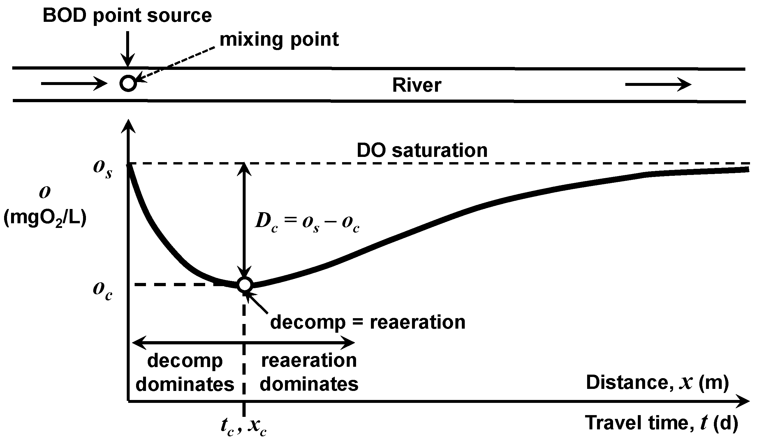
The ability of a waterbody to assimilate BOD point-source loadings will differ depending on the waterbody type. In the interest of simplicity, the following analysis focuses on the impact of a single point source of wastewater into a river with constant downstream flow, geometry, and temperature (Figure 4). The seminal water-quality model developed by Streeter and Phelps [1] is employed to compute the oxygen concentration at locations downstream of the mixing point as a function of the mixing-point BOD concentration. For steady-state conditions, zero initial oxygen deficit at the mixing point, no BOD settling losses, and minimal plant activity, the model is
where o = dissolved oxygen concentration (mgO2/L), L0 = concentration of biochemical oxygen demand (BOD) at the mixing point (mgO2/L), kd = deoxygenation rate (/d), ka = reaeration rate (/d), and t = travel time below the mixing point (defined as t = 0). Note that given a constant velocity, U (m/d), the distance downstream of the waste discharge, x (m), is linearly related to travel time by x = Ut.
As depicted in Figure 4, Equation (6) generates the classic dissolved oxygen sag with a minimum or “critical” oxygen concentration at the travel time (or downstream distance) below the discharge where the oxygen loss due to decomposition balances oxygen replenishment due to atmospheric reaeration. This minimum “critical” oxygen concentration, oc (mgO2/L), will be the focus of the following effort to assess how a river’s BOD assimilative capacity depends on water temperature. By determining the mixing-point BOD concentration necessary to maintain the critical oxygen concentration at the water-quality standard, oxygen concentration at all other travel time/locations will be higher than the water-quality standard.
2.5. Critical Oxygen Concentration
The oxygen deficit, D (mgO2/L), is the difference between the saturation oxygen concentration and the dissolved oxygen concentration at a specific travel time or distance below the mixing point
Comparison of Equations (6) and (7) shows that the last term of Equation (6) is, in fact, D.
Inspection of Equation (6) indicates that the relationship of the oxygen concentration to the BOD mixing-point concentration depends solely on three temperature-dependent parameters: oxygen saturation (os), the decomposition rate (kd), and the reaeration rate (ka). Fair [2] manipulated Equation (6) to determine the critical oxygen deficit in terms of those three parameters. Under the simplifying assumptions (i.e., zero mixing-point oxygen deficit, no BOD settling losses, and minimal plant activity) the critical oxygen deficit, Dc (mgO2/L), can be computed as [10]
Fair [2] also recognized that Equation (8) could be simplified further by defining the dimensionless ratio of the reaeration rate to the deoxygenation rate as a new parameter
where f = the dimensionless self-purification constant or reaeration–deoxygenation ratio. By defining f, Fair cleverly reduced the relationship of the critical oxygen deficit to the BOD mixing-point concentration from three factors to two: oxygen saturation and the dimensionless self-purification constant (f). As listed in Table 2, f varies between about 0.5 for very sluggish backwaters to well above 20 for very high energy streams.
Equation (9) can be substituted into Equation (8) and the result manipulated to yield
Thus, the ratio of the critical deficit to the mixing-point BOD concentration depends exclusively on the self-purification constant. This dependency is depicted in Figure 5 where, for the most stagnant backwaters and sluggish streams, the critical oxygen deficit is about 50% of the mixing-point BOD concentration. As reaeration intensifies relative to decomposition, the impact on the mixing-point BOD drops by over a factor of five to 10% or lower for fast-flowing, highly aerated streams.
Given a water-quality standard, owq (mgO2/L), as the concentration that must be maintained to protect the river’s water quality (in our case, avoiding hypoxia), Equation (10) can be solved for Dc and substituted into Equation (7) with oc set to owq. The result can then be solved for the “sustainable” mixing-point BOD concentration as
with
where ψ = the mixing-point BOD concentration-to-deficit ratio (dimensionless). The mixing-point BOD is modified with a subscript “s” to indicate that it is a “sustainable” mixing-point BOD concentration that maintains enough oxygen to support the river’s desired water quality, owq.
Equation (11) provides a unique solution for how L0s is determined as the product of the mixing-point BOD-to-deficit ratio, which is solely dependent on the temperature-dependent self-purification ratio (f), and the desired critical deficit, which is the difference between the temperature-dependent saturation concentration (os) and the water-quality standard (owq). Thus, Equation (11) neatly separates the impact of the two temperature-dependent factors: oxygen saturation and self-purification that govern a river’s capacity to absorb oxygen-demanding pollutants.
It should be stressed that L0s is not the BOD concentration of the point source. Rather, it is the flow-weighted average of the river and the point-source BOD concentrations. As the stream becomes more effluent dominated, the mixing-zone concentration approaches the point-source concentration. For less effluent-dominated systems, dilution allows the discharge of higher point-source BOD loadings.
We have already explored the temperature dependence of saturation (Figure 1). The next step is to quantify the temperature dependency of the self-purification constant.
2.6. Temperature Effect on the Self-Purification Constant
The effect of temperature on rates are commonly modeled with the simplified Arrhenius equation [12]
where k(T) is the rate at the water temperature T (°C), and θ = an empirically derived dimensionless Arrhenius constant. A value of θ = 1 indicates that there is no temperature dependence. A value of θ above 1 means that the rate increases as temperature increases with higher values yielding a stronger effect. A value of θ below 1 indicates that the rate decreases as temperature increases with lower values yielding a stronger effect. Note that a more intuitive way to parameterize the temperature dependence of rates is Q10, which is defined as the ratio k(20)/k(10). The parameters θ and Q10 are related mathematically by
We have summarized the Arrhenius model parameters for the key reaction rates connected with dissolved oxygen levels in natural waters in Table 3. Note that along with the rates used in the Streeter–Phelps model, other rates are included relevant to two other important oxygen-determining processes: eutrophication and sediment oxygen demand.
For the rates comprising f, it is conventional to employ θd = 1.047 and θa = 1.024 for carbonaceous BOD decomposition (kd) and reaeration (ka), respectively. Converting to Q10, this means that for a 10 °C rise in temperature, CBOD decomposition would increase by about 60% whereas reaeration would increase by about 25%. The other common oxygen-demanding reaction, nitrification (kn), has a higher θn ≅ 1.07, which corresponds to a doubling for a 10 °C water temperature rise. Hence, rising water temperatures will have a greater impact on nitrification than on the oxidation of organic carbon (Figure 6a).
The three rates increase as temperature increases with organic carbon decomposition and nitrification being more strongly temperature dependent than reaeration. Thus, the temperature dependence of the organic carbon self-purification ratio can be quantified as
where θfc = the Arrhenius constant for self-purification due to CBOD oxidation (dimensionless), which is computed as [2]
For nitrification, the temperature dependence of the reduced NBOD oxidation ratio can be quantified as
where θfn = the Arrhenius constant for self-purification due to NBOD oxidation (dimensionless) is computed as
Because θfn < θfc, self-purification of nitrogen oxygen demand will be reduced more by rising water temperatures than for self-purification based on reduced nitrogen oxidation.
Figure 6b is a plot of Equations (15) and (17) versus temperature. These results are significant as they indicate that for both cases, as water temperature increases, the process that replenishes oxygen (ka) increases at a lower rate than the processes that remove oxygen (kd or kn). This means that both self-purification ratios will decline as future water temperatures increase. Expressed as Q10, for a 10 °C temperature rise, the CBOD self-purification ratio would decrease by 20%, and decrease by 36% for NBOD.
Now that the temperature dependence of f is established, the manner in which temperature affects the dimensionless mixing-point BOD concentration-to-deficit ratio can be explored (Equation (12)). Figure 7 is a plot of the ratio versus temperature for sea-level rivers with different values of the self-purification constant at 20 °C. For very stagnant or lower velocity systems (f ≤ 1), the impact of higher temperature is negligible. However, for higher velocity streams the impact is significant. Notice also that the impact of temperature change on nitrification is more pronounced than for organic carbon decomposition as would be anticipated by its larger Arrhenius constant.
2.7. Temperature Effect on Assimilative Capacity
The final piece of this puzzle is to examine the total impact of rising temperature on a river’s assimilative capacity. That is, as modeled by Equation (11), how will the sustainable mixing-point BOD concentration be influenced by the temperature dependencies of both saturation and self-purification?
Figure 8 shows how the sustainable mixing-point concentration for freshwater rivers at several elevations and self-purification constants varies with temperature. The effects of temperature and elevation are most pronounced for high-velocity rivers and streams. This is significant as most high-velocity systems occur in mountainous regions. Due to their high reaeration rates, such systems typically exhibit high self-purification constants and, consequently, can assimilate larger oxygen-demanding loads. This assimilation is greatest at low temperatures when oxidation rates are reduced proportionally more than the drop in reaeration.
Whereas they have the largest assimilation capacity for oxygen-demanding pollutants, systems with high self-purification constants are also the most sensitive to rising temperatures. Although this is reflected visually by the greater negative slopes for the higher f curves in Figure 8, the temperature sensitivity of the sustainable load directly can be quantified by applying the product rule to differentiate Equation (11) with respect to temperature
where the derivatives on the right-hand side can be evaluated numerically with Equation (5).
Equation (19) is very useful as it converts the product of the two factors Equation (11) to a summation of their respective contributions to the total sensitivity. Although both factors appear in the two terms, they merely serve to convert the variation of each factor (the derivatives) into their respective contributions to the total temperature sensitivity of the sustainable mixing-point BOD concentration.
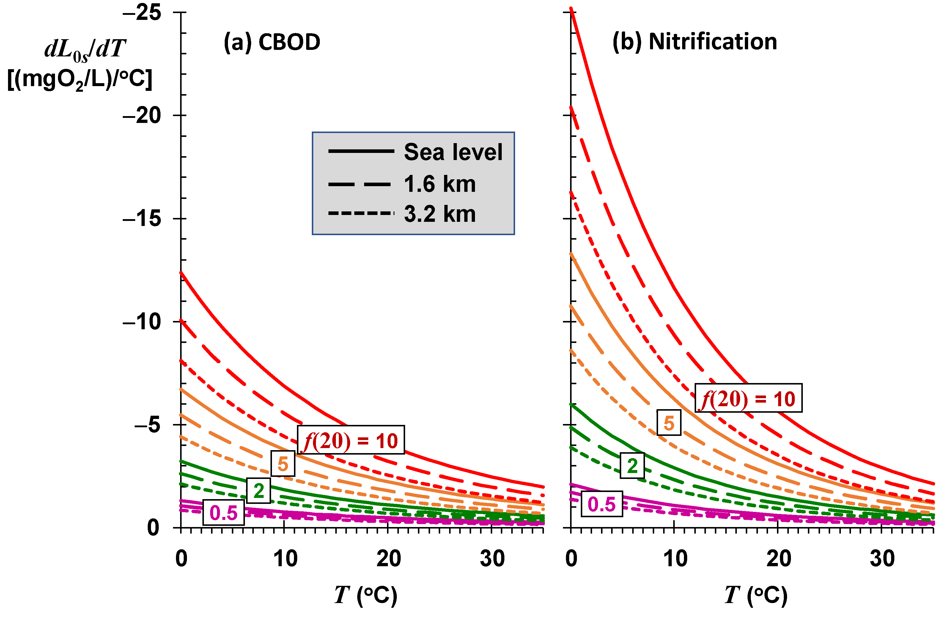
As depicted in Figure 9, the sustainable mixing-point concentrations for the most stagnant rivers (low f) are relatively insensitive to temperature variations. Although they have the highest assimilation capacities, rivers and streams with high self-purification constants (high f) are also the most sensitive to changing temperatures. For a high-elevation stream (elev = 1.6 km) with significant rapids and waterfalls (f(20) = 10) at a mean temperature of 17 °C, every degree Celsius of temperature rise reduces the sustainable mixing-point concentration by approximately 3.8 mgO2/L of CBOD.
We can take the analysis one step further by normalizing Equation (19) by dividing it by dL0s/dT and multiplying the result by 100% to yield
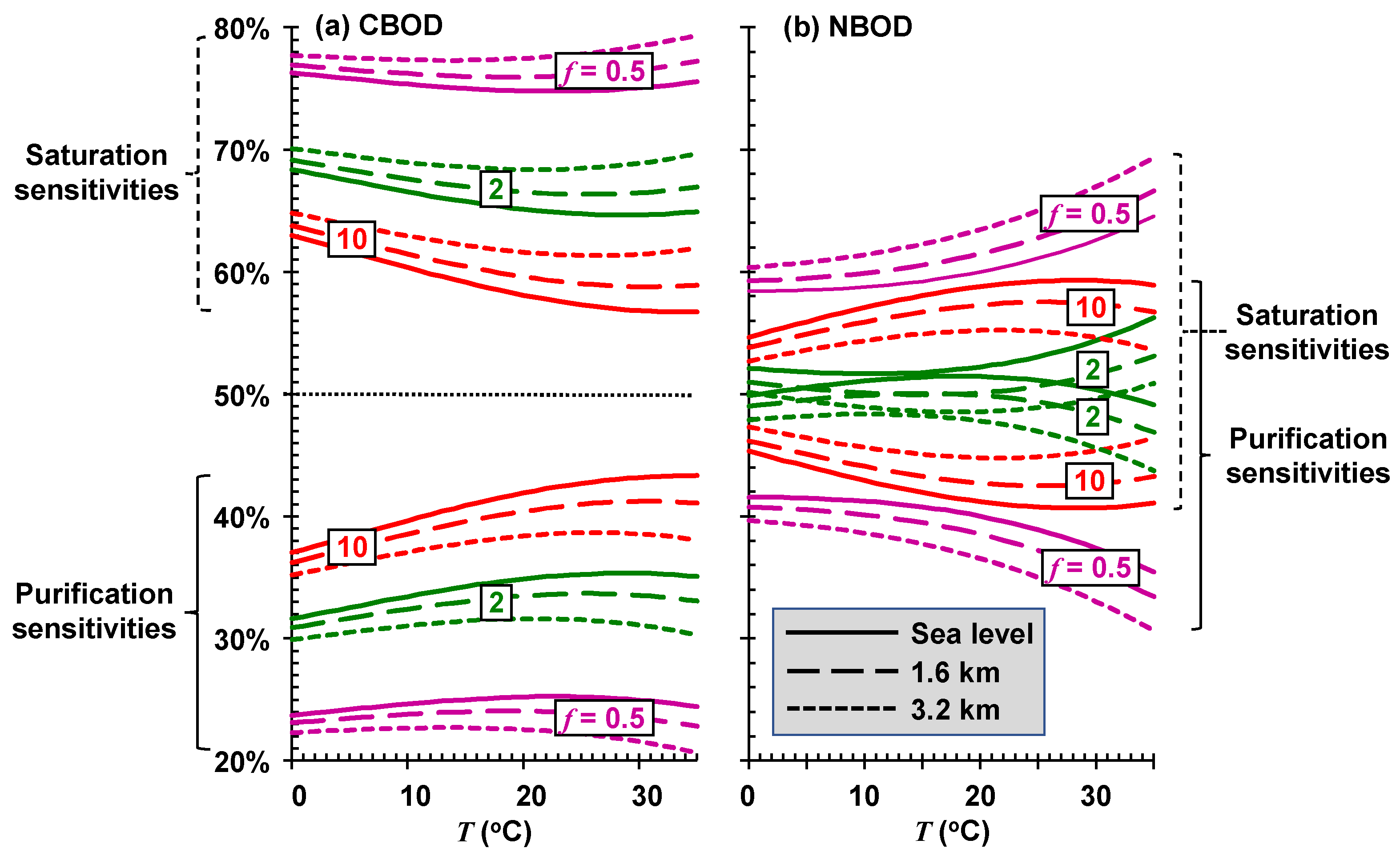
Thus, the sensitivity of the sustainable mixing-point concentration is separated into the percentages due to saturation and self-purification. These components can be evaluated for different river types (f) at different elevations (elev) and plotted versus temperature (Figure 10).
For CBOD, the total sustainable mixing-point concentration (Figure 10a) of very stagnant systems (f = 0.5) is primarily dictated by their sensitivity to saturation reductions. Sensitivity drops from about 78% at sea level to about 75% at an elevation of 3.2 km. Saturation sensitivity also dominates the high-velocity systems (f = 10), but at a reduced proportion of about 60%. Although saturation is dominant for CBOD, self-purification is still significant, especially for fast-flowing systems.
For NBOD, although the total sustainable mixing-point concentration (Figure 10b) for very stagnant stagnant systems is also more highly impacted by oxygen saturation reductions, the effect is less pronounced than for CBOD (~60%). For the high-velocity systems (f = 10), the sensitivity of the total sustainable load of reduced nitrogen is more equally dependent on both saturation and self-purification. For the fastest systems, self-purification actually becomes more dominant.
3. Discussion
We have employed a very simple steady-state model to provide a “10-km view” of the impact of global warming on river oxygen dynamics. Although the Streeter–Phelps model was very useful for management in the pre-computer era, it has been supplanted by much more comprehensive and complex models made possible by the widespread access and evolution of digital computers starting in the 1960s [17,18,19,20]. Although it is no longer used for management tasks such as wasteload allocations, the Streeter–Phelps model is a fundamentally sound parsimonious model that is still valuable for exploring the type of global questions addressed in the current paper.
3.1. Caveats
Because they are limited to a small number of parameters, parsimonious models often provide a means to draw broad general conclusions that can be very difficult to identify with more realistic but highly parameterized models [21] and, in some cases, they can also be preferable for practical model applications [22,23,24]. This follows the tradition of using parsimonious models to understand major facets of the dissolved oxygen problem [2,3,4] as well as other water-quality problems [22,25].
In so doing, a myriad of other facets of future oxygen-related water quality have been neglected. Several of these relate to the simplifying assumptions of Equation (6): steady-state conditions, zero initial oxygen deficit at the mixing point, no BOD settling losses, and minimal plant activity.
For example, the simplified analysis employed in this paper does not address the time-variable impacts of climate change on oxygen. Combined sewer overflows of oxygen-demanding wastes from urban catchments should intensify due to less-frequent high-intensity storms [26,27] that could lead to short-term anoxia, the magnitude and duration of which would be exacerbated by warmer water temperatures.
Our focus on BOD means that other major processes that impact oxygen have been neglected; most notably, eutrophication and sediment–water exchange of oxygen and nutrients. Incorporation of both these multifaceted processes requires much more complex non-linear models, which would preclude the simple analytical solutions employed in the present analysis to develop broad, global conclusions. For the time being, it should be noted that both processes have important rates with Arrhenius constants of a magnitude similar to NBOD (~1.07) and, hence, would exhibit the same high temperature sensitivity. For example, the diel oxygen variations due to plant photosynthesis (θ = 1.066) would tend to amplify diurnal dissolved oxygen swings and, hence, would lead to lower critical oxygen concentrations just before sunrise. Although analyzing these processes is beyond the scope of the current contribution, separate analyses could be devoted to quantifying the impact of warming on these two critical processes. The issue of diel water quality will be investigated in the second part of this paper [6].
The assumption of zero initial deficit at the mixing point has several deficiencies. First, unless diffusers are used, there is typically a mixing “zone” rather than a mixing “point” where the BOD loading enters the river. Except for wide rivers, there will come a downstream distance relatively close to the discharge point where the discharge would be well mixed across the stream width. Further, there are both simple equations [28,29] and more complex, mechanistic frameworks [30] to estimate the distance at which complete mixing is attained. Second, although the deficit can be near zero at the discharge point, it is more likely that it is not. Although the Streeter–Phelps framework can accommodate a non-zero deficit at the mixing-point, this would add an additional dimension that was unnecessary for the present analysis.
Finally, although we hold to our general conclusions regarding rivers and streams, global warming will impact the dissolved oxygen concentrations of all the planet’s surface waters. As noted previously, lakes and estuaries will be threatened by lowered oxygen saturation levels in the same way as rivers. However, particularly due to their different physics, reduced saturation as well as self-purification will differ in their ultimate effect.
Rather than being caused by allochthonous (externally produced) BOD from sewage discharges, oxygen problems in thermally stratified lakes and reservoirs are typically due to autochthonous (internally produced) BOD due to settling plant matter decaying in the hypolimnion. Although point-source sewage discharges can certainly cause hypoxia in tidal rivers and estuaries, they are often located at the downstream end of large watersheds. Hence, along with direct point loadings, they also receive significant amounts of plant nutrients due to non-point agricultural runoff in their watersheds. Furthermore, their intricate transport regimes caused by advective freshwater flow, tides, and salinity stratification must be accounted for.
3.2. Need for High-Temperature Experiments for Biochemical Rates
The temperature dependence of most of the rates used in management-oriented water-quality models were established in the 20th century. Up until the 1970s, the models focused on simulating the impact of untreated urban sewage on the oxygen and bacteria levels in natural waters. After 1970, attention was directed towards other problems including eutrophication, toxics, and acid rain. Thus, most of the rates were developed before climate change and global warming were recognized.
Today, as water temperatures rise beyond levels experienced in the past, there is a case to be made that the temperature dependence of model rates should be revisited with a focus on higher temperatures. For example, it has long been recognized that cyanobacteria, an important component of harmful algal blooms, thrive at higher temperatures than other algal groups [31,32]. Thus, it has been suggested that experiments be conducted to better quantify the impact of very high water temperatures on the growth and respiration rates of important algal species [31].
This reexamination at higher temperatures even extends to the rates employed in this paper. Because it is dependent on oxygen diffusivity in water, reaeration at higher temperatures is straightforward to compute. However, the impact of high temperature on biochemical rates such as CBOD deoxygenation, nitrification, and denitrification might merit further study.
3.3. Shallow, High-Energy Streams
In an interesting paper, Ulseth and colleagues noted that very high-gradient streams can have extremely large gas transfer coefficients [11]. They concluded that gas exchange in rivers and streams exists in two states. Whereas turbulent diffusion drives gas transfer velocity in low-energy streams, turbulence entrains air bubbles in high-energy streams leading to larger transfer rates than would be expected based on diffusion alone.
It is also well known [13] that shallow streams typically exhibit higher decomposition rates (1 to 5/d) than deeper rivers (0.05–0.5/d). The usual explanation for this is that bed processes, such as bottom bacterial biofilms and hyporheic flow, would have a greater effect on shallow than on deeper systems [10]. Furthermore, smaller streams often exhibit significant dead zones that tend to enhance kd and kn by increasing the residence time of the water caught up in the zones [25]. For hyporheic flow, this also prevents atmospheric gas transfer.
Because the current study relies on the dimensionless ratio, f, these observations do not negate our major conclusions. Nevertheless, shallow streams with very steep slopes deserve further study. Not only does this relate to the current study’s focus on BOD assimilative capacity but also on topics such as quantifying their contribution to greenhouse gas emissions [11].
3.4. The Special Threat of Global Warming to Salmonid Fisheries
As mentioned in the discussion of Figure 9, the largest sustainable BOD assimilative capacity occurs in very fast-flowing rivers at colder temperatures. As noted previously, such systems are typically located in mountainous regions where water temperatures are generally colder than for lower elevation rivers. Furthermore, excluding rivers located in a few densely populated, high-elevation metropolitan areas (notably the megacities, Bogota, Columbia, and Mexico City), human population density is typically much less than for lower elevation rivers [33].
Of course, as population continues to grow, some high-altitude, non-urban watersheds are beginning to be developed for recreation and tourism. This is particularly true in the Western Hemisphere and should increase in the future [6]. Regardless, one might conclude that such rivers are presently less vulnerable to global warming.
Nevertheless, because they are colder, highly aerated, and less developed than lowland rivers, these systems are often prime habitats for prized, cold-water gamefish such as the salmonids (most notably, trout, char, and salmon). Consequently, if the desire is to protect a cold-water fishery, it will be necessary to do more than merely avoiding hypoxia. Rather, as depicted in Figure 3, a standard of approximately 5–6 mgO2/L would be appropriate. This would reduce the stream’s assimilative capacity slack by 3–4 mgO2/L relative to the hypoxia standard of 2 mgO2/L employed in this paper. Furthermore, recall that high-elevation systems will also have lower saturation values due to the reduced partial pressure of oxygen gas at altitude.
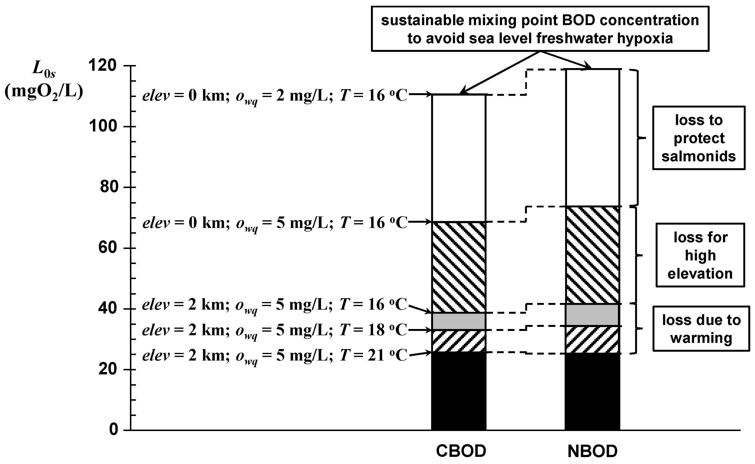
The impact of all these factors can be illustrated by an example. As depicted in Figure 11, the model is used to compute the sustainable mixing-point BOD concentrations for several scenarios. The total height of each bar corresponds to the base case of avoiding hypoxia for a fast-flowing, freshwater sea-level river. A series of cases are indicated that progressively lower the allowable mixing-point BOD concentration to (a) support a salmonid fishery, (b) move the river to high elevation, and (c) subject it to climate-induced warming.
The key parameters for the base case are f20 = 10, owq = 2 mgO2/L, elev = 0, and T = 16 °C. The subsequent scenarios are:
- Scenario 1. Raise the owq to 5 mgO2/L to support a salmonid fishery.
- Scenario 2. Move the river to a high elevation by setting elev = 2 km.
- Scenario 3. Increase the critical (usually late summer) water temperature to T = 18 °C (moderate) and 21 °C (high).
First, the oxygen-saturation slack is increased by raising the water-quality standard (owq) from 2 to 5 mgO2/L (Figure 3) to support a salmonid fishery. This change reduces the allowable mixing-point concentration by about 38%. Next, the river’s elevation is increased to 2 km, which reduces the allowable mixing-point concentration by an additional 27% for a total of 65%. Note that up to this point, the reductions in CBOD and NBOD are identical. Finally, the river’s maximum temperature is increased to 2 °C and 5 °C, which reduces the sustainable mixing-point oxygen by an additional 4.5% and 10%, respectively. Thus, protecting a salmonid fishery in a fast-flowing mountain stream reduces the sustainable mixing-point oxygen concentration by about 90% as compared with the base case of merely avoiding hypoxia for a fast-flowing, sea-level system.
4. Conclusions
In summary, a modeling analysis has been developed to draw broad and general conclusions regarding the effect of climate-induced rising water temperatures on the ability of the earth’s rivers to assimilate oxygen-demanding pollutants. For rivers and streams with a single point source, the impact of rising water temperature on BOD assimilative capacity depends on the interplay of two independent factors: the waterbody’s dissolved oxygen saturation, and its self-purification.
Using standard formulations, it is shown that the sea-level freshwater saturation concentration declines monotonically with rising water temperatures with the highest rate of decrease occurring at low temperatures. The saturation is lowered additionally by salinity as well as reduced atmospheric pressure at elevations above sea level. Hence, the impact of temperature on the slack is more pronounced for marine and high-elevation systems. Although this analysis centers on rivers and streams, these conclusions regarding oxygen saturation are independent of waterbody type and hence would apply to all the world’s waters including lakes, estuaries, and marine waters.
Beyond the reduction of saturation, a waterbody’s capacity to safely assimilate oxygen-demanding pollution is also determined by the relative magnitudes of oxygen replenishment due to gas transfer and its depletion due to BOD oxidation. This dependence is parameterized by a dimensionless self-purification constant consisting of the ratio of the reaeration rate to the deoxygenation rate (f). The two processes comprising self-purification increase as temperature increases with the decomposition rates (kd for CBOD and kn for NBOD) increasing faster than the reaeration rate (ka). Thus, as water temperatures rise, self-purification declines. Hence, global warming will not only reduce assimilative capacity by lowering oxygen saturation but also by increasing oxygen depletion faster than reaeration.
As a final step in the analysis, the combined effect of the reductions in saturation and self-purification are examined. To do this, the critical maximum deficit (i.e., the maximum saturation slack) is set equal to the DO saturation minus a desired DO water-quality standard corresponding to hypoxia. The maximum deficit equation can then be solved for the mixing-point BOD concentration as the product of the saturation slack and a dimensionless mixing-point BOD concentration-to-deficit ratio, which is solely dependent on self-purification.
We plotted the sustainable mixing-point concentration for freshwater rivers at several elevations and self-purification constants versus temperature. The effects of temperature and elevation are most pronounced for high-velocity rivers and streams. This is significant as a large fraction of high-velocity rivers and streams occur in mountainous regions. Due to their high reaeration rates, such systems typically exhibit high self-purification constants and, consequently, can assimilate higher oxygen-demanding loads. This assimilation is greatest at low temperatures when oxidation rates are reduced relatively more than the drop in reaeration.
The sustainable mixing-point concentrations for the most stagnant rivers are relatively insensitive to temperature variations. Although they have the highest assimilation capacities, rivers and streams with high self-purification constants are also the most sensitive to changing temperatures. For a high-elevation stream (elev = 1.6 km) with significant rapids and waterfalls (f(20) = 10) at a mean temperature of 17 °C, every degree Celsius of temperature rise reduces the sustainable mixing-point concentration by approximately 3.8 mgO2/L of CBOD.
Using the multiplication rule for differentiation, the total sustainable mixing-point concentration sensitivity is disaggregated into the percentages due to saturation and to self-purification. For stagnant systems, the total sustainable mixing-point concentration for CBOD is primarily dictated by its sensitivity to saturation reductions due to rising temperatures. Saturation sensitivity also dominates the faster flowing rivers and streams, but at a reduced proportion of about 60%. Although the total sustainable mixing-point concentration of reduced nitrogen for stagnant rivers is also more highly impacted by oxygen saturation reductions, the effect is less pronounced than for CBOD. For the faster flowing rivers and streams, the sensitivity of the total sustainable load of reduced nitrogen is more equally dependent on both saturation and self-purification.
In conclusion, the study that yielded the Streeter and Phelps model was published in 1925 [1]. Hence, 2025 will mark the 100th anniversary of the field of surface water-quality modeling. Thus, it is gratifying that this seminal model still provides a means to draw some useful conclusions regarding the impact of global warming on river water quality.
Nevertheless, as mentioned in the prior section outlining caveats, this study has just scratched the surface of the myriad ways that climate change will threaten the future water quality of surface waterbodies. Although the analysis of a few of these problems might be amenable to the type of parsimonious approach described in this paper, most will require process-based models to adequately gain insights [34,35]. In the second part of this paper [6], this is accomplished by analyzing the oxygen problem for the high-elevation Bogota River in Columbia using a complex, process-based water-quality model. This second paper will address many of the facets of the oxygen problem that were not addressed by the admittedly simple parsimonious model used in the current paper. These will include the impact of rising water temperature on sediment–water interactions, plant photosynthesis and respiration, and diel oxygen swings.
Author Contributions
Conceptualization, S.C.C.; methodology, S.C.C. and G.B.M.; software, S.C.C. and L.A.C.; validation, G.B.M. and L.A.C.; formal analysis, S.C.C.; writing—original draft preparation, S.C.C.; writing—review and editing, G.B.M. and L.A.C.; visualization, S.C.C. All authors have read and agreed to the published version of the manuscript.
Funding
This research received no external funding.
Institutional Review Board Statement
Not applicable.
Informed Consent Statement
Not applicable.
Data Availability Statement
Not applicable.
Acknowledgments
This paper is dedicated to our colleague, dear friend, and one of the unsung heroes of water-quality modeling: James J. Fitzpatrick. Jim was a great consulting engineer who made several major contributions to our field, most notably to estuary eutrophication modeling [36] and sediment diagenesis modeling [37]. He was also co-author on the first version of the EPA WASP model [38]. We miss “Fitz” very much. We thank the three anonymous reviewers for their constructive criticism and positive suggestions. The first author (S.C.C.) developed the basic ideas for this paper as a Visiting Scientist at the National Institute of Water and Atmospheric Research (NIWA), Christchurch, New Zealand in 2020.
Conflicts of Interest
The authors declare no conflict of interest.
Nomenclature
| Symbol | Definition | Units |
| D | DO deficit | mgO2/L |
| Dc | critical DO deficit | mgO2/L |
| elev | elevation | km |
| f | self-purification constant or reaeration–deoxygenation ratio | dimensionless |
| fc | readily oxidizable organic carbon (CBOD) self-purification ratio | dimensionless |
| fn | reduced nitrogen (NBOD) self-purification ratio | dimensionless |
| ka | reaeration rate | /d |
| kd | deoxygenation rate | /d |
| kn | nitrification rate | /d |
| L0 | BOD concentration at the mixing point | mgO2/L |
| L0s | sustainable BOD concentration at the mixing point | mgO2/L |
| o | DO concentration | mgO2/L |
| oc | critical DO concentration | mgO2/L |
| os | DO saturation concentration | mgO2/L |
| osf | the DO saturation concentration of sea-level freshwater | mgO2/L |
| owq | DO water-quality standard | mgO2/L |
| S | salinity | ppt |
| t | travel time below the mixing point | d |
| T | water temperature | °C |
| U | velocity | m/d |
| x | distance downstream of the waste discharge | m |
| ψ | mixing-point BOD concentration-to-oxygen deficit ratio | dimensionless |
| ϕelev | fractional reduction of freshwater sea-level saturation due to elevation | dimensionless |
| ϕS | the fractional reduction of freshwater sea-level saturation due to salinity | dimensionless |
| θa | Arrhenius constant for reaeration | dimensionless |
| θd | Arrhenius constant for CBOD oxidation | dimensionless |
| θfc | Arrhenius constant for self-purification due to CBOD oxidation | dimensionless |
| θfn | Arrhenius constant for self-purification due to NBOD oxidation | dimensionless |
| θn | Arrhenius constant for NBOD oxidation | dimensionless |
References
- Streeter, H.W.; Phelps, E.B. A Study of the Pollution and Natural Purification of the Ohio River. III. Factors Concerned in the Phenomena of Oxidation and Reaeration; Public Health Bulletin 146; U.S. Public Health Service: Washington, DC, USA, 1925. [Google Scholar]
- Fair, G.M. The dissolved oxygen sag—An analysis. Sew. Works J. 1939, 11, 445–461. [Google Scholar]
- Hydroscience, Inc. Simplified Mathematical Modeling of Water Quality; U.S. Environmental Protection Agency, Water Quality Office: Washington, DC, USA, 1971. [Google Scholar]
- McBride, G.B. Nomographs for rapid solutions for the Streeter Phelps equations. Water Pollut. Control Fed. 1982, 54, 378–384. [Google Scholar]
- American Public Health Association (APHA). Standard Methods for the Examination of Water and Wastewater, 23rd ed.; Rice, E.W., Baird, R.B., Eaton, A.D., Eds.; APHA: Washington, DC, USA, 2017. [Google Scholar]
- Camacho, L.A.; Chapra, S.C. Impact of global warming on the oxygen concentration and BOD assimilative capacity of the world’s rivers: 2. Application to a high elevation river. Water 2021. in preparation. [Google Scholar]
- Chapra, S.C.; Clough, D.E. Applied Numerical Methods with Python for Engineers and Scientists; WCB/McGraw-Hill: New York, NY, USA, 2021. [Google Scholar]
- Di Toro, D.M. Sediment Flux Modeling; Wiley-Interscience: New York, NY, USA, 2001. [Google Scholar]
- Vaquer-Sunyer, R.; Duarte, C.M. Thresholds of hypoxia for marine biodiversity. Proc. Natl Acad. Sci. USA 2008, 105, 15452–15457. [Google Scholar] [CrossRef] [PubMed] [Green Version]
- Chapra, S.C. Surface Water Quality Modeling; McGraw-Hill: New York, NY, USA, 1997. [Google Scholar]
- Ulseth, A.J.; Hall, R.O., Jr.; Boix Canadell, M.; Madinger, H.L.; Niayifar, A.; Battin, T.J. Distinct air–water gas exchange regimes in low- and high-energy streams. Nat. Geosci. 2019, 12, 259–263. [Google Scholar] [CrossRef]
- Arrhenius, S.Z. Über die Reaktionsgeschwindigkeit bei der Inversion von Rohrzucker durch Säuren. Phys. Chem. 1889, 4, 226–248. [Google Scholar]
- Thomann, R.V.; Mueller, J.A. Principles of Surface Water Quality Modeling and Control; Harper-Collins: New York, NY, USA, 1987. [Google Scholar]
- Zison, S.W.; Mills, W.B.; Deimer, D.; Chen, C.W. Rates, Constants and Kinetic Formulations in Surface Water Quality Modeling; ERL, EPA/600/3-78-105; U.S. EPA, ORD: Athens, GA, USA, 1985. [Google Scholar]
- Churchill, M.A.; Elmore, H.A.; Buckingham, R.A. Prediction of stream reaeration rates. J. Sanit. Eng. Div. Proc. Am. Soc. Civ. Eng. 1962, 88, 1–46. [Google Scholar] [CrossRef]
- Eppley, R.W. Temperature and phytoplankton growth in the sea. Fish. Bull. 1972, 70, 1063–1085. [Google Scholar]
- Brown, L.C.; Barnwell, T.O. The Enhanced Stream Water Quality Models QUAL2E and QUAL2E-UNCAS: Documentation and User Manual; US EPA/600/3-87/007; US EPA: Washington, DC, USA, 1987; 127p. [Google Scholar]
- Reichert, P.; Borchardt, D.; Henze, M.; Rauch, W.; Shanahan, P.; Somlyódy, L.; Vanrolleghem, P. River water quality model no. 1 (RWQM1): II. Biochemical process equations. Water Sci. Technol. 2001, 43, 329–338. [Google Scholar] [CrossRef]
- Pelletier, G.J.; Chapra, S.C.; Tao, H. QUAL2Kw—A framework for modeling water quality in streams and rivers using a genetic algorithm for calibration. Environ. Model. Softw. 2006, 21, 419–425. [Google Scholar] [CrossRef]
- Wool, T.; Ambrose, R.B.; Martin, J.L.; Comer, A. WASP 8: The next generation in the 50-year evolution of USEPA’s water quality model. Water 2020, 12, 1398. [Google Scholar] [CrossRef]
- Chapra, S.C.; Flynn, K.F.; Rutherford, J.C. Parsimonious model for assessing nutrient impacts on periphyton-dominated streams. J. Environ. Eng. 2014, 140, 04014014. [Google Scholar] [CrossRef]
- Chapra, S.C.; Canale, R.P. Long-term phenomenological model of phosphorus and oxygen in stratified lakes. Water Res. 1991, 25, 707–715. [Google Scholar] [CrossRef]
- Wagener, T.; Lees, M.J.; Wheater, H.S. A framework for the development and application of parsimonious hydrological models. In Mathematical Models of Large Watershed Hydrology; Singh, V.P., Frevert, D., Eds.; Water Resources Publications LLC: Highlands Ranch, CO, USA, 2002; Volume 1, pp. 91–140. [Google Scholar]
- Mannina, G.; Viviani, G. A parsimonious dynamic model for river water quality assessment. Water Sci. Technol. 2010, 61, 607–618. [Google Scholar] [CrossRef] [PubMed]
- Chapra, S.C.; Runkel, R.L. Modeling impact of storage zones on stream water quality. J. Environ. Eng. 1999, 125, 415–419. [Google Scholar] [CrossRef]
- Groisman, P.Y.; Knight, R.W.; Easterling, D.R.; Karl, T.R.; Hegerl, G.C.; Razuvaev, V.N. Trends in intense precipitation in the climate record, J. Clim. 2005, 18, 1326–1350. [Google Scholar] [CrossRef]
- Nilsen, V.; Lier, J.A.; Bjerkholt, J.T.; Lindholm, O.G. Analysing urban floods and combined sewer overflows in a changing climate. J. Water Clim. Chang. 2011, 2, 260–271. [Google Scholar] [CrossRef]
- Fischer, H.B.; List, E.J.; Koh, R.C.Y.; Imberger, J.; Brooks, N. Mixing in Inland and Coastal Waters; Academic: San Diego, CA, USA, 1979. [Google Scholar]
- Rutherford, J.C. River Mixing; Wiley: Chichester, UK, 1994. [Google Scholar]
- Doneker, R.L.; Jirka, G.H. CORMIX User Manual; EPA-823-K-07-001; Environmental Research Laboratory, U.S. Environmental Protection Agency: Athens, GA, USA, 2007. [Google Scholar]
- Paerl, H.W.; Huisman, J. Blooms like it hot. Science 2008, 320, 57–58. [Google Scholar] [CrossRef] [Green Version]
- Paerl, H.; Otten, T. Harmful cyanobacterial blooms: Causes, consequences, and controls. Microb. Ecol. 2013, 65, 995–1010. [Google Scholar] [CrossRef]
- Small, C.; Cohen, J. Continental physiography, climate, and the global distribution of human population. Curr. Anthropol. 2004, 45, 269–277. [Google Scholar] [CrossRef]
- Chapra, S.C.; Boehlert, B.; Fant, C.; Henderson, J.; Mills, D.; Mas, D.M.L.; Rennels, L.; Jantarasami, L.; Martinich, J.; Strzepek, K.M.; et al. Climate change impacts on harmful algal blooms in U.S. freshwater. Environ. Sci. Technol. 2017, 51, 8933–8943. [Google Scholar] [CrossRef] [PubMed]
- Gooseff, M.N.; Strzepek, K.; Chapra, S.C. Modeling the effects of climate change on water temperature downstream of a shallow reservoir, Lower Madison River, MT. Clim. Chang. 2005, 68, 331–353. [Google Scholar] [CrossRef]
- Thomann, R.V.; Fitzpatrick, J.J. Calibration and Verification of a Mathematical Model of the Eutrophication of the Potomac Estuary; Department of Environmental Services, Government of the District of Columbia: Washington, DC, USA, 1982. [Google Scholar]
- Di Toro, D.M.; Fitzpatrick, J.J. Chesapeake Bay Sediment Flux Model; Contract Report EL-93-2; U.S. Army Corps of Engineers Waterways Experiment Station: Vicksburg, MI, USA, 1993. [Google Scholar]
- Di Toro, D.M.; Fitzpatrick, J.J.; Thomann, R.V. Documentation for Water Quality Analysis Simulation Program (WASP) and Model Verification Program (MVP); EPA-600/3-81-044; Environemt Research Lab, ORD, US EPA: Duluth, MN, USA, 1983. [Google Scholar]
Figure 1.
Dissolved oxygen saturation (mgO2/L) versus temperature (°C) for sea-level freshwater, seawater, and a very high-elevation freshwater lake. The vertical arrows specify the difference between the saturation concentration and an oxygen concentration standard corresponding to hypoxia. This is termed assimilative capacity “slack”; that is, the maximum allowable dissolved oxygen deficit that can be generated before hypoxia occurs. The plot indicates how the saturation and the assimilative capacity “slack” of all three systems decrease with rising water temperature.

Figure 2.
The rate of change of oxygen saturation with respect to temperature ((mgO2/L)/°C) versus temperature (°C) for freshwater at three elevations (solid lines) and seawater (dashed line). The vertical dotted lines indicate four key temperatures.
Figure 2.
The rate of change of oxygen saturation with respect to temperature ((mgO2/L)/°C) versus temperature (°C) for freshwater at three elevations (solid lines) and seawater (dashed line). The vertical dotted lines indicate four key temperatures.

Figure 3.
A dissolved oxygen concentration (mgO2/L) scale showing several key levels related to establishing oxygen concentration targets needed to maintain ecosystem health and protect designated uses.
Figure 3.
A dissolved oxygen concentration (mgO2/L) scale showing several key levels related to establishing oxygen concentration targets needed to maintain ecosystem health and protect designated uses.

Figure 4.
The classic Streeter–Phelps model showing the dissolved oxygen sag in a river below a point source of BOD.
Figure 4.
The classic Streeter–Phelps model showing the dissolved oxygen sag in a river below a point source of BOD.

Figure 5.
Plot of the ratio of critical deficit to the sustainable mixing-point concentration of carbonaceous BOD versus the self-purification constant at 20 °C. The “sustainable mixing-point concentration” is the level to maintain the downstream critical oxygen concentration at the value where hypoxia begins.

Figure 6.
(a) Plot of the ratio of the Streeter–Phelps reaction rates normalized to the value at 20 °C versus temperature. The steepness of the slopes means that the rates connected with oxygen depletion (kd and kn) are more strongly impacted by temperature than the rate connected with oxygen replenishment (ka). (b) Plot of the ratio of the self-purification constants normalized to the value at 20 °C versus temperature. The monotonic declines mean that self-purification is reduced because reaeration increases at a slower rate than oxidation. Hence, the assimilation of oxygen-demanding pollutants due to self-purification will decrease as the planet’s natural surface waters warm. The curves also indicate that the decrease for NBOD will be greater than that for CBOD.

Figure 7.
Plot of ψ, the ratio of the sustainable mixing-point BOD concentration (L0s) to the critical deficit (Dc) versus temperature for sea-level rivers with different values of the 20 °C self-purification constant.
Figure 7.
Plot of ψ, the ratio of the sustainable mixing-point BOD concentration (L0s) to the critical deficit (Dc) versus temperature for sea-level rivers with different values of the 20 °C self-purification constant.

Figure 8.
Plot of the mixing-point concentration versus temperature for freshwater rivers at several elevations and self-purification constants.
Figure 8.
Plot of the mixing-point concentration versus temperature for freshwater rivers at several elevations and self-purification constants.

Figure 9.
Plot of the temperature sensitivity of the sustainable mixing-point concentration as a function of temperature for freshwater rivers at several elevations and self-purification constants.
Figure 9.
Plot of the temperature sensitivity of the sustainable mixing-point concentration as a function of temperature for freshwater rivers at several elevations and self-purification constants.

Figure 10.
Percentage contributions due to the saturation and self-purification of the temperature sensitivity of the sustainable mixing-point concentration of (a) CBOD and (b) NBOD as a function of temperature for freshwater rivers at several elevations and self-purification constants (f = 0.5: very stagnant; f = 2: large, moderate velocity streams; f = 10: high-velocity streams with rapids and waterfalls).

Figure 11.
Bar chart depicting sustainable mixing-point BOD concentration to avoid sea-level freshwater hypoxia along with reductions due to protecting salmonid fisheries, moving from sea level to high elevation, and warming water temperatures due to climate change.
Figure 11.
Bar chart depicting sustainable mixing-point BOD concentration to avoid sea-level freshwater hypoxia along with reductions due to protecting salmonid fisheries, moving from sea level to high elevation, and warming water temperatures due to climate change.


Table 1.
The rate of change of oxygen saturation with respect to temperature ((mgO2/L)/°C) for selected temperatures (°C) for freshwater at three elevations and seawater.
Table 1.
The rate of change of oxygen saturation with respect to temperature ((mgO2/L)/°C) for selected temperatures (°C) for freshwater at three elevations and seawater.
| T (°C) | Freshwater | Ocean | ||
|---|---|---|---|---|
| elev = 0 S = 0 | elev = 1.6 S = 0 | elev = 3.2 S = 0 | elev = 0 S = 35 | |
| 0 | −0.414 | −0.341 | −0.279 | −0.297 |
| 5 | −0.330 | −0.272 | −0.222 | −0.240 |
| 10 | −0.266 | −0.219 | −0.179 | −0.196 |
| 15 | −0.218 | −0.179 | −0.147 | −0.162 |
| 20 | −0.181 | −0.149 | −0.122 | −0.135 |
| 25 | −0.152 | −0.125 | −0.103 | −0.115 |
| 30 | −0.131 | −0.108 | −0.088 | −0.100 |
| 35 | −0.114 | −0.094 | −0.077 | −0.088 |
| 40 | −0.101 | −0.083 | −0.068 | −0.079 |
Table 2.
Approximate values for the self-purification constant for CBOD at 20 °C as originally suggested by Fair [2] and supplemented by very high-energy streams [11].
| Nature of Receiving Water | Range of f(20) |
|---|---|
| (a) Backwaters | 0.5–1 |
| (b) Sluggish streams | 1–1.5 |
| (c) Large, low-velocity streams | 1.5–2 |
| (d) Large, high-velocity streams | 2–3 |
| (e) Swift streams | 3–5 |
| (f) Rapids, waterfalls | 5–20 |
| (g) Extremely high-energy and high-gradient streams | > 20 |
Table 3.
Values of the temperature correction factors for the simple Arrhenius model for key reaction rates connected with dissolved oxygen levels in natural waters.
Table 3.
Values of the temperature correction factors for the simple Arrhenius model for key reaction rates connected with dissolved oxygen levels in natural waters.
| Reaction | θ | Range of θ | Q10 | Reference |
|---|---|---|---|---|
| CBOD decay | 1.047 | (1.02–1.09) | 1.58 | [1,13] |
| NBOD decay | 1.07 | (1.055–1.1) | 2.16 | [13,14] |
| Reaeration | 1.024 | (1.005–1.03) | 1.27 | [13,15] |
| Phytoplankton growth | 1.066 | 1.89 | [16] | |
| Phytoplankton respiration | 1.08 | 2.16 | [13,14] | |
| Sediment oxygen demand | 1.065 | (1.04–1.13) | 1.88 | [8,14] |
| Biological “rule of thumb” | 1.07 | 1.97 |
Publisher’s Note: MDPI stays neutral with regard to jurisdictional claims in published maps and institutional affiliations. |
© 2021 by the authors. Licensee MDPI, Basel, Switzerland. This article is an open access article distributed under the terms and conditions of the Creative Commons Attribution (CC BY) license (https://creativecommons.org/licenses/by/4.0/).
Share and Cite
MDPI and ACS Style
Chapra, S.C.; Camacho, L.A.; McBride, G.B. Impact of Global Warming on Dissolved Oxygen and BOD Assimilative Capacity of the World’s Rivers: Modeling Analysis. Water 2021, 13, 2408. https://doi.org/10.3390/w13172408
AMA Style
Chapra SC, Camacho LA, McBride GB. Impact of Global Warming on Dissolved Oxygen and BOD Assimilative Capacity of the World’s Rivers: Modeling Analysis. Water. 2021; 13(17):2408. https://doi.org/10.3390/w13172408
Chicago/Turabian StyleChapra, Steven C., Luis A. Camacho, and Graham B. McBride. 2021. "Impact of Global Warming on Dissolved Oxygen and BOD Assimilative Capacity of the World’s Rivers: Modeling Analysis" Water 13, no. 17: 2408. https://doi.org/10.3390/w13172408
Note that from the first issue of 2016, this journal uses article numbers instead of page numbers. See further details here.