
Proposal of a Laboratory-Scale Anaerobic Biodigester for Introducing the Monitoring and Sensing Techniques, as a Potential Learning Tool in the Fields of Carbon Foot-Print Reduction and Climate Change Mitigation

 , , , and
Abstract
:1. Introduction
2. Materials and Methods
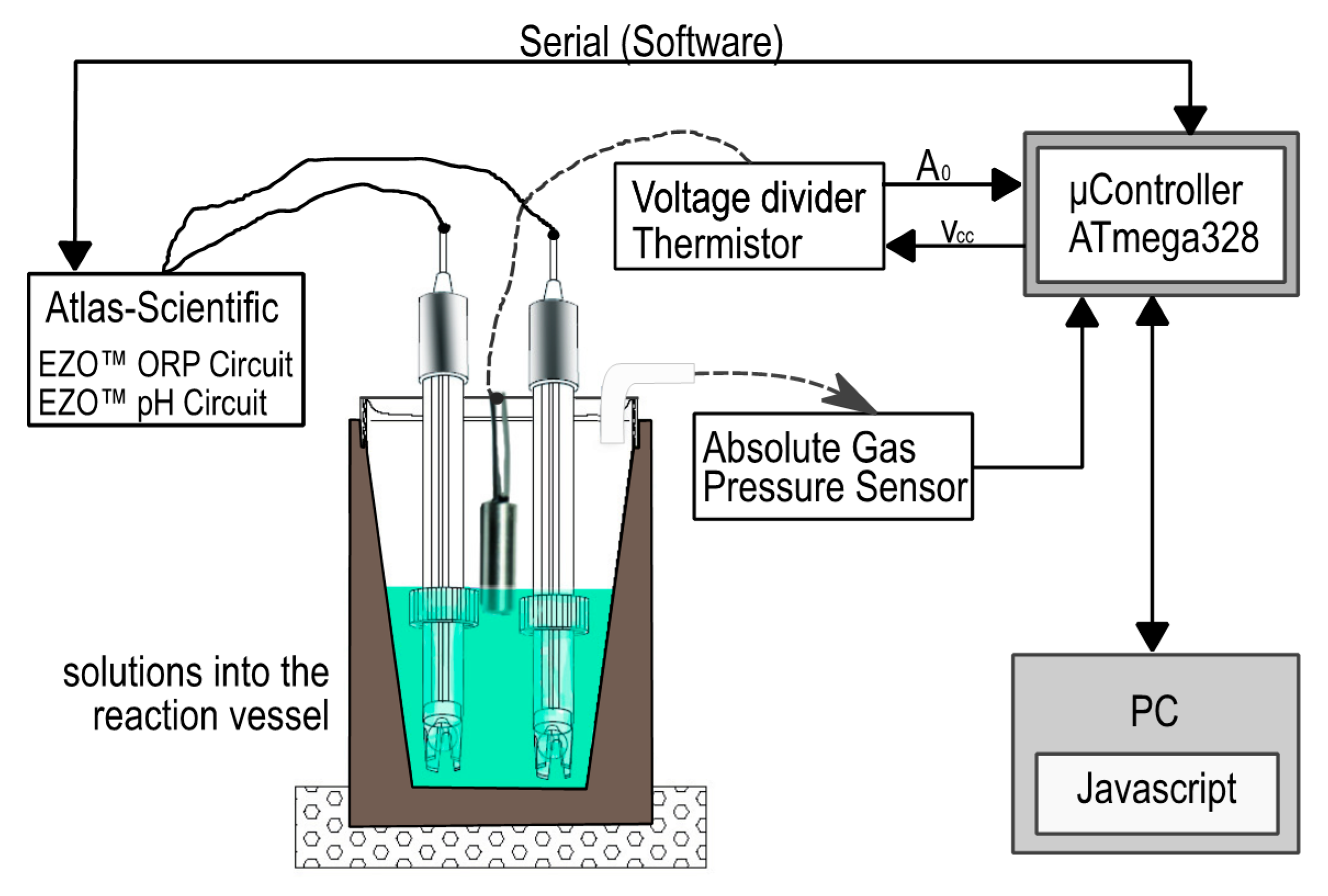
2.1. Diagram of the Laboratory Reactor
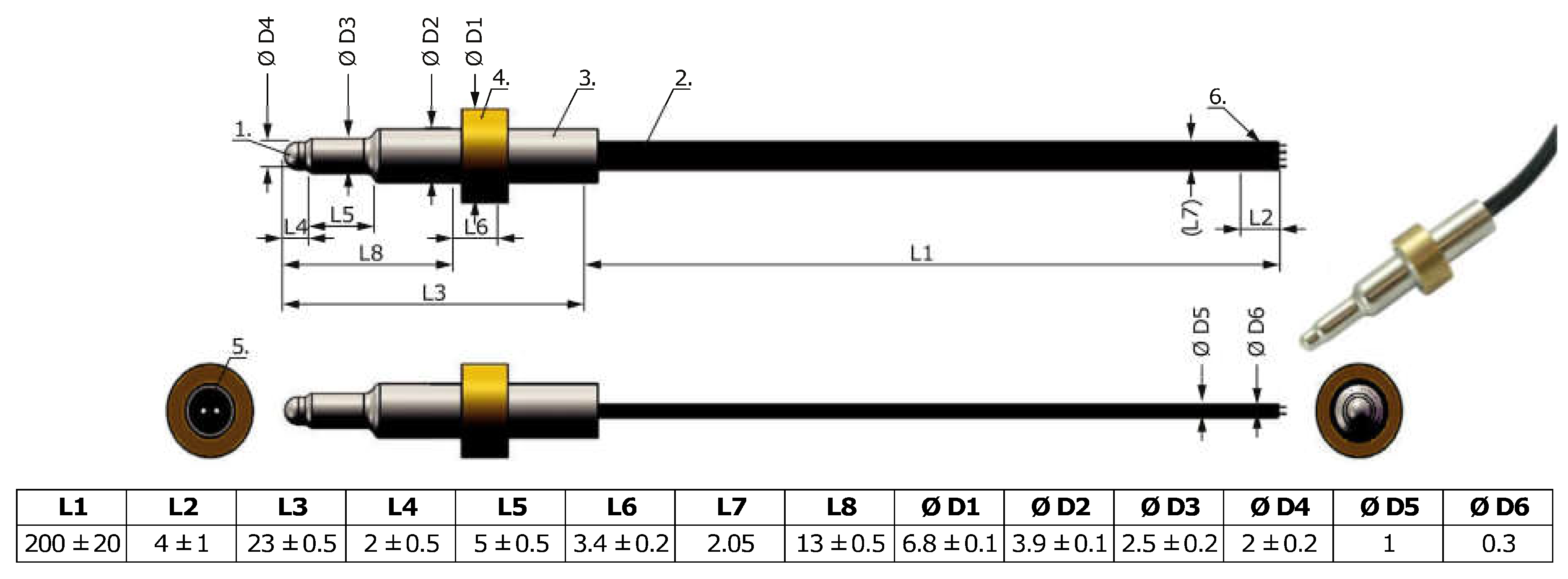
2.1.1. Digestion System
- pH Sensor: Scientific Grade Silver/Silver Chloride pH), 10 sensor with a response speed of 95% in one second.
- Absolute Pressure Sensor: Phidgets mod. 1141-0—Absolute Sensor of gas pressure from 15 to 115 kPa [49,50]. This is a high-level sensor with analogue input, with input proportional to the of the environment. The pressure measurement for this sensor is 15 kPa. The formula used to translate the sensor value into pressure was the following [2,51,52]:
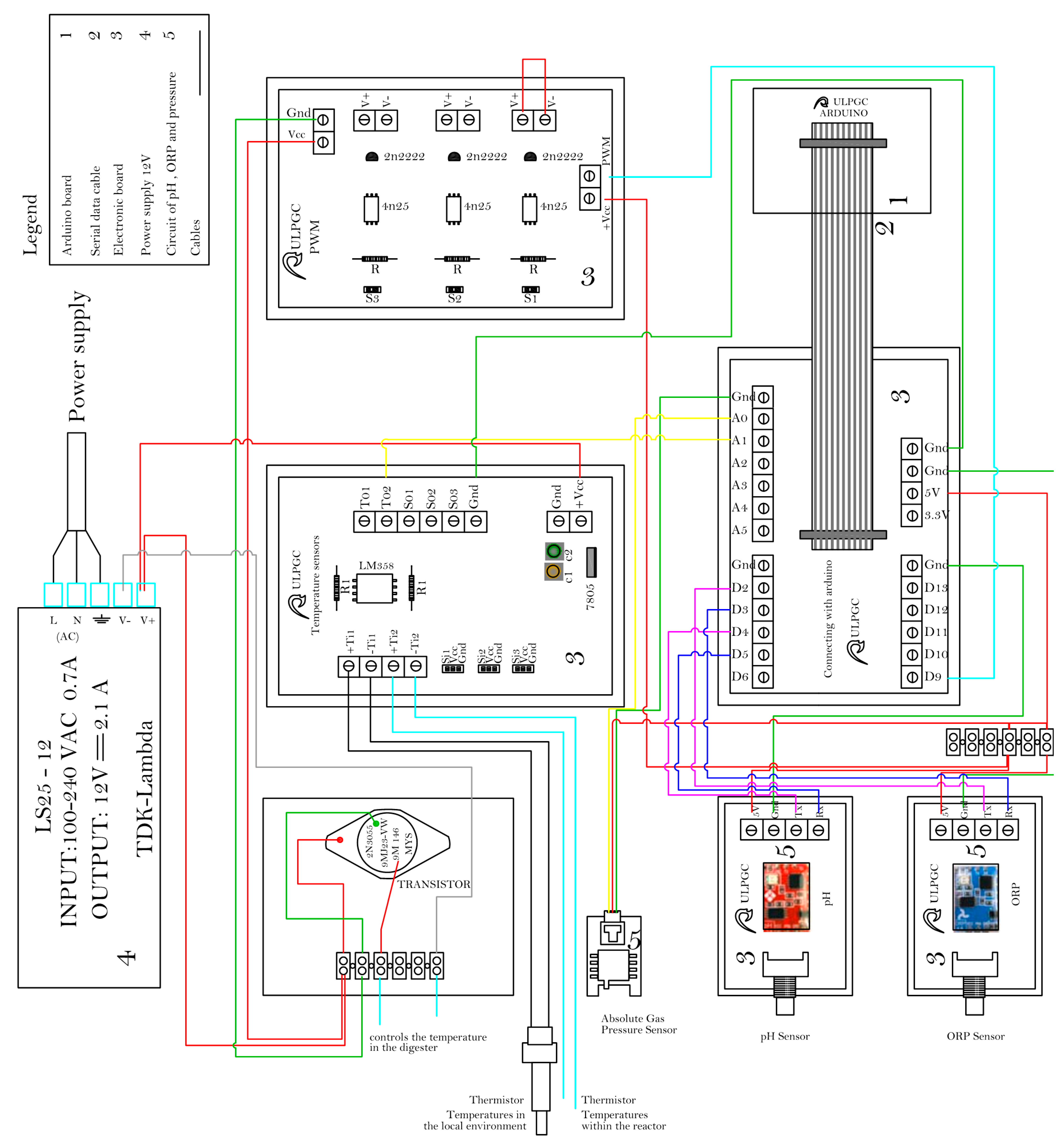
2.1.2. Circuits and Control System
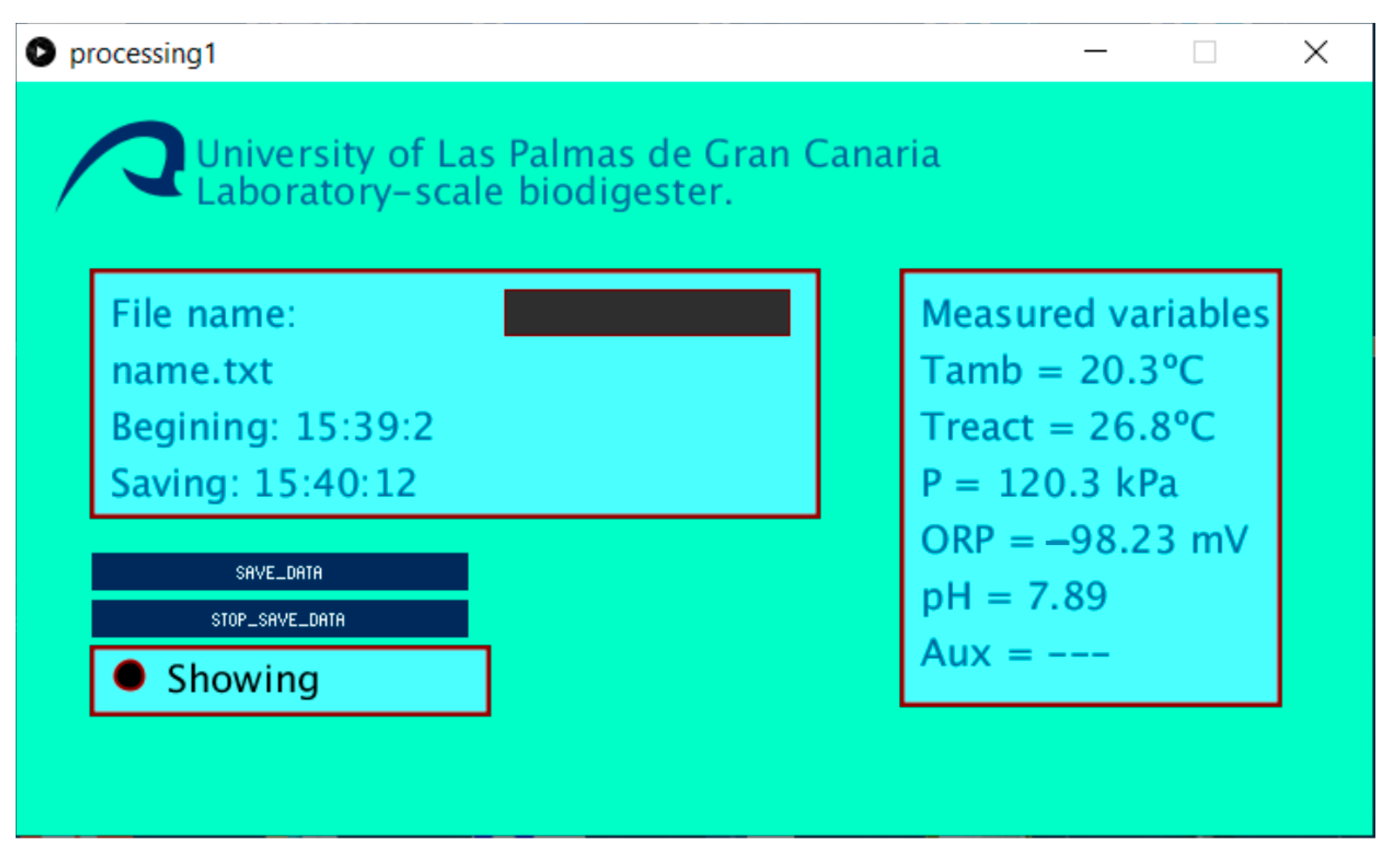
2.1.3. Computer System, Communication Interface, and Software
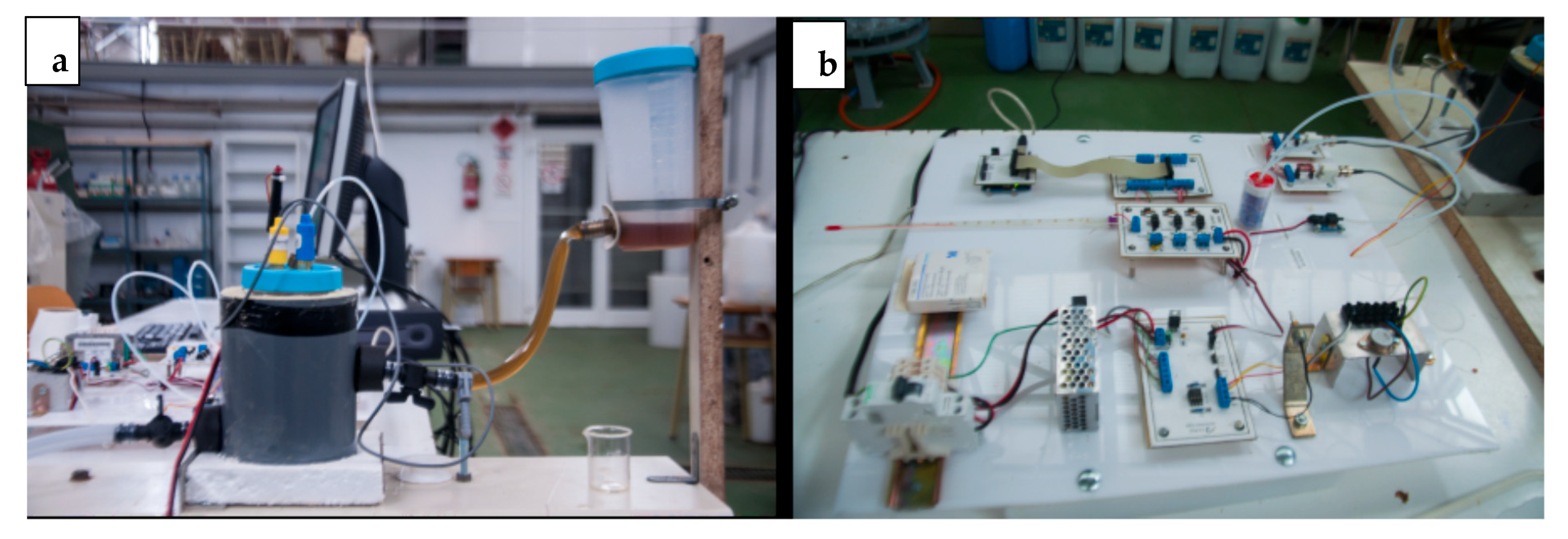
2.1.4. Auxiliary Equipment and Laboratory Material
2.2. Preparation and Testing
2.2.1. Preparation of the Substrate
2.2.2. Microbial Inoculum
2.2.3. Control and Saving Data
3. Results
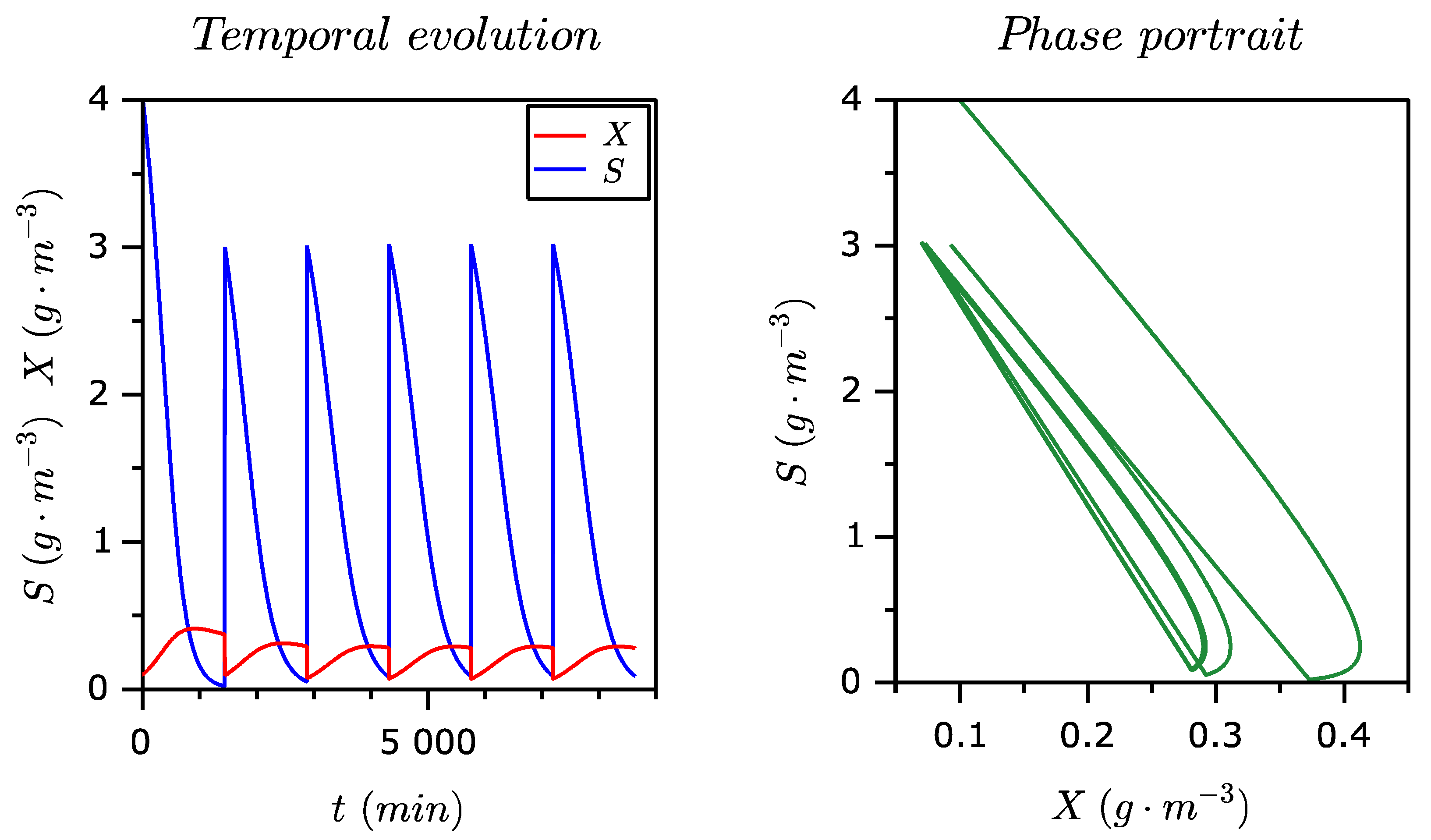
3.1. Digestion Model
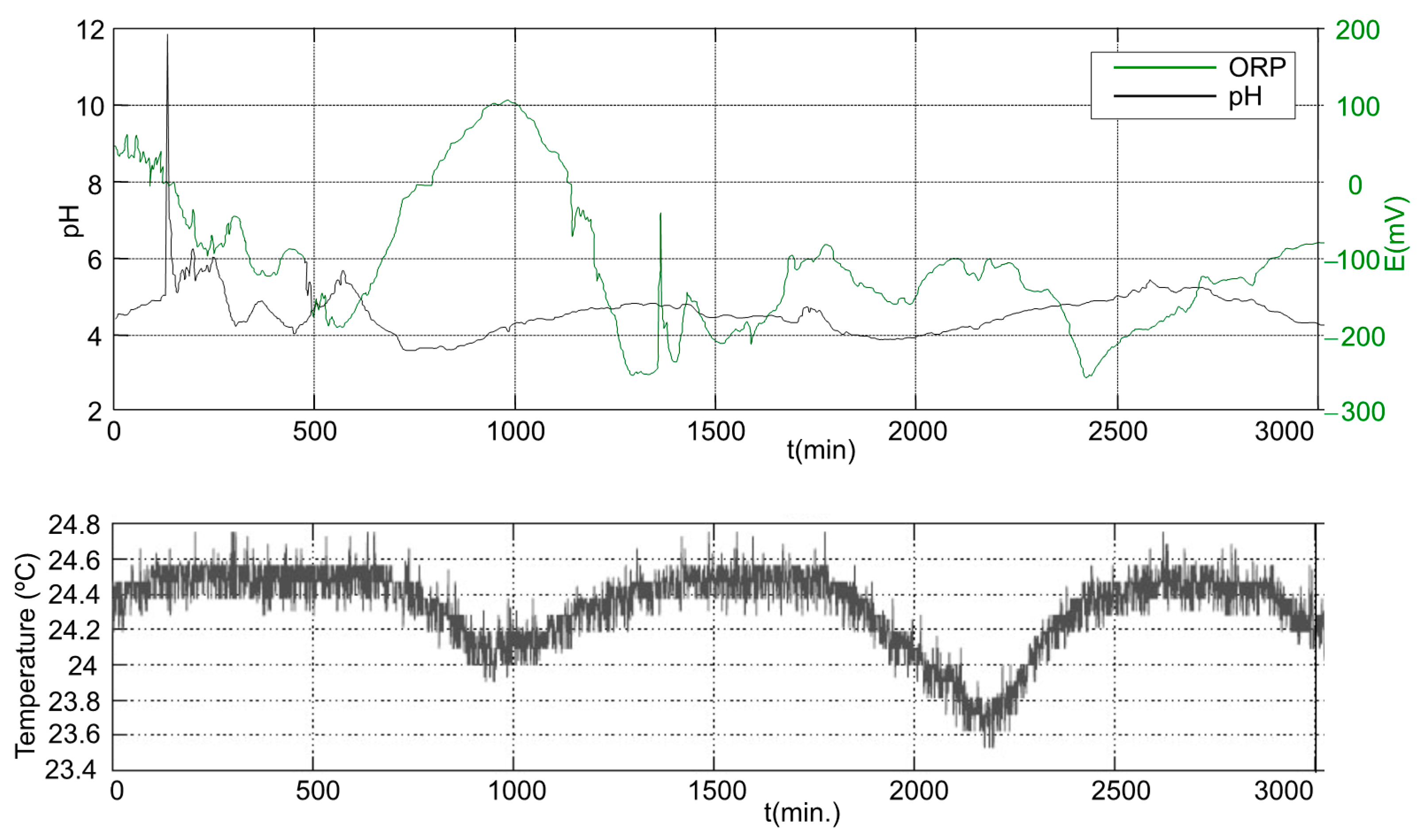
3.2. Anaerobic Digester Start-Up and Operation
3.2.1. First Stage
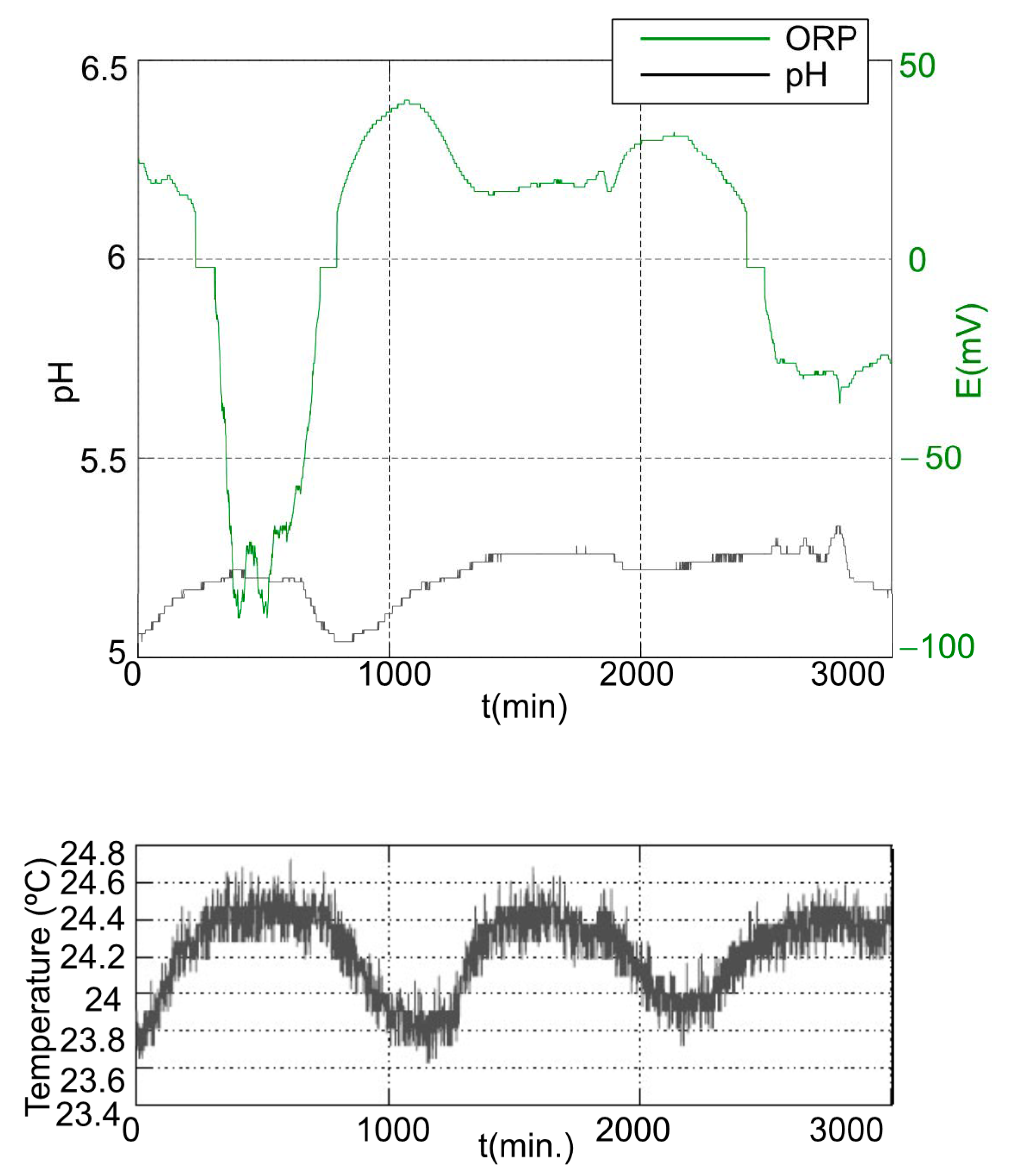
3.2.2. Second Stage
3.2.3. Third Stage
4. Conclusions
Author Contributions
Funding
Institutional Review Board Statement
Informed Consent Statement
Data Availability Statement
Acknowledgments
Conflicts of Interest
Appendix A. SCILAB Source Code
Appendix B. Microcontroller Source Code (Arduino)
Appendix C. Processing Source Code
References
- Brito-Espino, S.; Ramos-Martín, A.; Pérez-Báez, S.O.; Mendieta-Pino, C.; Leon-Zerpa, F. A Framework Based on Finite Element Method (FEM) for Modelling and Assessing the Affection of the Local Thermal Weather Factors on the Performance of Anaerobic Lagoons for the Natural Treatment of Swine Wastewater. Water 2021, 13, 882. [Google Scholar] [CrossRef]
- Cano, E.; Ruiz, J.G.; Garcia, I.A. Integrating a learning constructionist environment and the instructional design approach into the definition of a basic course for embedded systems design. Comput. Appl. Eng. Educ. 2015, 23, 36–53. [Google Scholar] [CrossRef]
- Garcia, I.A.; Cano, E.M. Designing and implementing a constructionist approach for improving the teaching-learning process in the embedded systems and wireless communications areas. Comput. Appl. Eng. Educ. 2014, 22, 481–493. [Google Scholar] [CrossRef]
- Available online: http://www.atago.net/Spanish/download.htmlRX-7000i (accessed on 11 June 2021).
- Refractómetro Digital Automático Atago. Available online: http://www.atago.net/Spanish/download.html (accessed on 14 June 2021).
- Jagnow, G.; Dawind, W. Biotecnología: Introducción Con Experimentos Modelo; Acribia S.A.: Zaragoza, Spain, 1991. [Google Scholar]
- Liu, C.-G.; Xue, C.; Lin, Y.-H.; Bai, F.-W. Redox potential control and applications in microaerobic and anaerobic fermentations. Biotechnol. Adv. 2013, 31, 257–265. [Google Scholar] [CrossRef]
- Madsen, M.; Holm-Nielsen, J.B.; Esbensen, K.H. Monitoring of anaerobic digestion processes: A review perspective. Renew. Sustain. Energy Rev. 2011, 15, 3141–3155. [Google Scholar] [CrossRef] [Green Version]
- Mekic, E.; Djokic, I.; Zejnelagic, S.; Matovic, A. Constructive approach in teaching of voip in line with good laboratory and manufacturing practice. Comput. Appl. Eng. Educ. 2016, 24, 277–287. [Google Scholar] [CrossRef]
- Pantaleo, A.; De Gennaro, B.; Shah, N. Assessment of optimal size of anaerobic co- digestion plants: An application to cattle farms in the province of bari (Italy). Renew. Sustain. Energy Rev. 2013, 20, 57–70. [Google Scholar] [CrossRef]
- Atlas Scientific. Atlas Scientific. Orpatlas. Available online: https://atlas-scientific.com/?gclid=EAIaIQobChMIvbPk8o3Z8gIVied3Ch03AgqaEAAYASAAEgKLzPD_BwE (accessed on 19 July 2021).
- Sorathia, K.; Servidio, R. Learning and experience: Teaching tangible interaction & edutainment. Procedia—Soc. Behav. Sci. 2012, 64, 265–274. [Google Scholar]
- Taylhardat Arjona, L.A. El biogas. Fundamentos e Infraestructura Rural; Instituto de Ingenieria Agri- cola; Facultad de Agronomia U.C.V: Maracay, Venezuela, 1986. [Google Scholar]
- Leon, F.; Ramos, A.; Vaswani, J.; Mendieta, C.; Brito, S. Climate Change Mitigation Strategy through Membranes Replacement and Determination Methodology of Carbon Footprint in Reverse Osmosis RO Desalination Plants for Islands and Isolated Territories. Water 2021, 13, 293. [Google Scholar] [CrossRef]
- Products for USB Sensing and Control. Products for Usb Sensing and Control. Available online: www.phidgets.com (accessed on 1 July 2021).
- Parralejo, A.; Royano, L.; González, J.; González, J. Small scale biogas production with animal excrement and agricultural residues. Ind. Crops Prod. 2019, 131, 307–314. [Google Scholar] [CrossRef]
- Holm-Nielsen, J.; Seadi, T.A.; Oleskowicz-Popiel, P. The future of anaerobic digestion and biogas utilization. Bioresour. Technol. 2009, 100, 5478–5484. [Google Scholar] [CrossRef]
- Park, J.H.; Park, J.H.; Lee, S.H.; Jung, S.P.; Kim, S.H. Enhancing anaerobic digestion for rural wastewater treatment with granular activated carbon (GAC) supplementation. Bioresour. Technol. 2020, 315, 123890. [Google Scholar] [CrossRef] [PubMed]
- Jiang, Y.; Bebee, B.; Mendoza, A.; Robinson, A.K.; Zhang, X.; Rosso, D. Energy footprint and carbon emission reduction using off-the-grid solar-powered mixing for lagoon treatment. J. Environ. Manag. 2018, 205, 125–133. [Google Scholar] [CrossRef] [PubMed]
- Duan, N.; Zhang, D.; Khoshnevisan, B.; Kougias, P.G.; Treu, L.; Liu, Z.; Lin, C.; Liu, H.; Zhang, Y.; Angelidaki, I. Human waste anaerobic digestion as a promising low-carbon strategy: Operating performance, microbial dynamics and environmental footprint. J. Clean. Prod. 2020, 256, 120414. [Google Scholar] [CrossRef]
- Mendieta-Pino, C.A.; Ramos-Martin, A.; Perez-Baez, S.O.; Brito-Espino, S. Management of slurry in Gran Canaria Island with full-scale natural treatment systems for wastewater (NTSW). One year experience in livestock farms. J. Environ. Manag. 2019, 232, 666–678. [Google Scholar]
- Muga, H.; Mihelcic, J. Sustainability of wastewater treatment technologies. J. Environ. Manag. 2008, 88, 437–447. [Google Scholar] [CrossRef]
- Wu, B.; Chen, Z. An integrated physical and biological model for anaerobic lagoons. Bioresour. Technol. 2011, 102, 5032–5038. [Google Scholar] [CrossRef] [PubMed]
- Wu, B. Advances in the use of CFD to characterize, design and optimize bioenergy systems. Comput. Electron. Agric. 2013, 93, 195–208. [Google Scholar] [CrossRef]
- Donoso-Bravo, A.; Sadino-Riquelme, C.; Gómez, D.; Segura, C.; Valdebenito, E.; Hansen, F. Modelling of an anaerobic plug-flow reactor. Process analysis and evaluation approaches with non-ideal mixing considerations. Bioresour. Technol. 2018, 260, 95–104. [Google Scholar]
- Rajeshwari, K.; Balakrishnan, M.; Kansal, A.; Lata, K.; Kishore, V. State-of-the-art of anaerobic digestion technology for industrial wastewater treatment. Renew. Sustain. Energy Rev. 2000, 4, 135–156. [Google Scholar] [CrossRef]
- Lauwers, J.; Appels, L.; Thompson, I.P.; Degrève, J.; Impe, J.F.V.; Dewil, R. Mathematical modelling of anaerobic digestion of biomass and waste: Power and limitations. Prog. Energy Combust. 2013, 39, 383–402. [Google Scholar] [CrossRef] [Green Version]
- Wade, M.; Harmand, J.; Benyahia, B.; Bouchez, T.; Chaillou, S.; Cloez, B. Perspectives in mathematical modelling for microbial ecology. Ecol. Model. 2016, 321, 64–74. [Google Scholar] [CrossRef]
- Batstone, D.; Keller, J.; Angelidaki, I.; Kalyuzhnyi, S.; Pavlostathis, S.; Rozzi, A.; Sanders, W.; Siegrist, H.; Vavilin, V. The IWAAnaerobic Digestion Model No 1 (ADM1). Water Sci. Technol. 2002, 45, 65–73. Available online: https://library.lanl.gov/cgi-bin/getfile?00285556.pdf (accessed on 1 September 2020). [CrossRef]
- Kleerebezem, R.; van Loosdrecht, M.C.M. Critical analysis of some concepts proposed in ADM1. Water Sci. Technol. 2006, 54, 51–57. [Google Scholar] [CrossRef] [PubMed] [Green Version]
- Li, D.; Lee, I.; Kim, H. Application of the linearized ADM1 (LADM) to lab-scale anaerobic digestion system. J. Environ. Chem. Eng. 2021, 9, 105193. [Google Scholar] [CrossRef]
- Fleming, J.G. Novel Simulation of Anaerobic Digestion Using Computational Fluid Dynamics. Ph.D. Thesis, North Carolina State University, Raleigh, NC, USA, 2002. [Google Scholar]
- Goodarzi, D.; Sookhak Lari, K.; Mossaiby, F. Thermal effects on the hydraulic performance of sedimentation ponds. J. Water Process. Eng. 2020, 33, 101100. [Google Scholar] [CrossRef]
- Brito-Espino, S.; Ramos-Martín, A.; Pérez-Báez, S.; Mendieta-Pino, C. Application of a mathematical model to predict simultaneous reactions in anaerobic plug-flow reactors as a primary treatment for constructed wetlands. Sci. Total Environ. 2020, 713, 136244. [Google Scholar] [CrossRef]
- Mahmudul, H.; Rasul, M.; Akbar, D.; Narayanan, R.; Mofijur, M. A comprehensive review of the recent development and challenges of a solar-assisted biodigester system. Sci. Total Environ. 2021, 753, 141920. [Google Scholar] [CrossRef] [PubMed]
- Atelge, M.; Atabani, A.; Banu, J.R.; Krisa, D.; Kaya, M.; Eskicioglu, C.; Kumar, G.; Lee, C.; Yildiz, Y.; Unalan, S.; et al. A critical review of pretreatment technologies to enhance anaerobic digestion and energy recovery. Fuel 2020, 270, 117494. [Google Scholar] [CrossRef]
- Tumilar, A.S.; Milani, D.; Cohn, Z.; Florin, N.; Abbas, A. A Modelling Framework for the Conceptual Design of Low-Emission Eco-Industrial Parks in the Circular Economy: A Case for Algae-Centered Business Consortia. Water 2021, 13, 69. [Google Scholar] [CrossRef]
- Haßler, S.; Ranno, A.M.; Behr, M. Finite-element formulation for advection–reaction equations with change of variable and discontinuity capturing. Comput. Methods Appl. Mech. Eng. 2020, 369, 113171. [Google Scholar] [CrossRef]
- Mirza, I.A.; Akram, M.S.; Shah, N.A.; Imtiaz, W.; Chung, J.D. Analytical solutions to the advection-diffusion equation with Atangana-Baleanu time-fractional derivative and a concentrated loading. Alex. Eng. J. 2021, 60, 1199–1208. [Google Scholar] [CrossRef]
- Singh, S.; Bansal, D.; Kaur, G.; Sircar, S. Implicit-explicit-compact methods for advection diffusion reaction equations. Comput. Fluids 2020, 212, 104709. [Google Scholar] [CrossRef]
- Zeng, L.; Chen, G. Ecological degradation and hydraulic dispersion of contaminant in wetland. Ecol. Model. 2011, 222, 293–300. [Google Scholar] [CrossRef]
- Bozkurt, S.; Moreno, L.; Neretnieks, I. Long-term processes in waste deposits. Sci. Total Environ. 2000, 250, 101–121. [Google Scholar] [CrossRef]
- Song, L.; Li, P.W.; Gu, Y.; Fan, C.M. Generalized finite difference method for solving stationary 2D and 3D Stokes equations with a mixed boundary condition. Comput. Math. Appl. 2020, 80, 1726–1743. [Google Scholar] [CrossRef]
- Ukai, S. A solution formula for the Stokes equation in Rn+. Commun. Pure Appl. Math. 1987, 40, 611–621. [Google Scholar] [CrossRef] [Green Version]
- Reddy, J.; Gartling, D. The Finite Element Method in Heat Transfer and Fluid Dynamics, 3rd ed.; CRC Press: Boca Raton, FL, USA, 2010; pp. 1–483. [Google Scholar]
- Alvarez-Hostos, J.C.; Bencomo, A.D.; Puchi-Cabrera, E.S.; Fachinotti, V.D.; Tourn, B.; Salazar-Bove, J.C. Implementation of a standard stream-upwind stabilization scheme in the element-free Galerkin based solution of advection-dominated heat transfer problems during solidification in direct chill casting processes. Eng. Anal. Bound. Elem. 2019, 106, 170–181. [Google Scholar] [CrossRef]
- Guldentops, G.; Van Dessel, S. A numerical and experimental study of a cellular passive solar façade system for building thermal control. Sol. Energy 2017, 149, 102–113. [Google Scholar] [CrossRef]
- Lawrence, M.G. The Relationship between Relative Humidity and the Dewpoint Temperature in Moist Air: A Simple Conversion and Applications. Bull. Am. Meteorol. Soc. 2005, 86, 225–234. [Google Scholar] [CrossRef]
- Çengel, Y. Heat Transfer: A Practical Approach. In McGraw-Hill Series in Mechanical Engineering; McGraw Hill Books: London, UK, 2003. [Google Scholar]
- Walton, G.N. Thermal Analysis Research Program Reference Manual; NBSIR, Department of Energy, Office of Building Energy Research and Development: Washington, DC, USA, 1983. [Google Scholar]
- Monod, J. The Growth of Bacterial Cultures. Annu. Rev. Microbiol. 1949, 3, 371–394. [Google Scholar] [CrossRef] [Green Version]
- Rosso, L.; Lobry, J.; Flandrois, J. An Unexpected Correlation between Cardinal Temperatures of Microbial Growth Highlighted by a New Model. J. Theor. Biol. 1993, 162, 447–463. [Google Scholar] [CrossRef] [PubMed]
- Herus, V.A.; Ivanchuk, N.V.; Martyniuk, P.M. A System Approach to Mathematical and Computer Modeling of Geomigration Processes Using Freefem++ and Parallelization of Computations. Cybern Syst. Anal. 2018, 54, 284–292. [Google Scholar] [CrossRef]
- Donoso-Bravo, A.; Bandara, W.; Satoh, H.; Ruiz-Filippi, G. Explicit temperature-based model for anaerobic digestion: Application in domestic wastewater treatment in a UASB reactor. Bioresour. Technol. 2013, 133, 437–442. [Google Scholar] [CrossRef] [Green Version]
- Donoso-Bravo, A.; Retamal, C.; Carballa, M.; Ruiz-Filippi, G.; Chamy, R. Influence of temperature on the hydrolysis, acidogenesis and methanogenesis in mesophilic anaerobic digestion: Parameter identification and modeling application. Water Sci. Technol. 2009, 60, 9–17. [Google Scholar] [CrossRef]
- Wang, R.; Lv, N.; Li, C.; Cai, G.; Pan, X.; Li, Y.; Zhu, G. Novel strategy for enhancing acetic and formic acids generation in acidogenesis of anaerobic digestion via targeted adjusting environmental niches. Water Res. 2021, 193, 116896. Available online: https://www.sciencedirect.com/science/article/pii/S0043135421000944 (accessed on 23 June 2021). [CrossRef]
- Weißbach, M.; Drewes, J.E.; Koch, K. Application of the oxidation reduction potential (ORP) for process control and monitoring nitrite in a Coupled Aerobic-anoxic Nitrous Decomposition Operation (CANDO). Chem. Eng. J. 2018, 343, 484–491. Available online: https://www.sciencedirect.com/science/article/pii/S1385894718303929 (accessed on 30 June 2021). [CrossRef]
- Ao, T.; Chen, L.; Zhou, P.; Liu, X.; Li, D. The role of oxidation-reduction potential as an early warning indicator, and a microbial instability mechanism in a pilot-scale anaerobic mesophilic digestion of chicken manure. Renew. Energy 2021, 179, 223–232. Available online: https://www.sciencedirect.com/science/article/pii/S0960148121010521 (accessed on 1 July 2021). [CrossRef]


| Parameter | Value | Units |
|---|---|---|
| Resistence value at 25 °C | 10 K | Ω |
| Tolerance of R25 | ±3 | % |
| B25/85 (Beta) | 3984 | K |
| Temperatura range of operation | −25 to 105 | °C |
| Stage | Date | Feeding/Evacuation | Brix Grades | Remarks | ||
|---|---|---|---|---|---|---|
| (mL) | 1st Lecture | 2nd Lecture | Average | |||
| 1 | 13 June | 300 | 20.30 | 20.30 | ||
| 2 | 18 June | 75 | 20.31 | 20.29 | 20.30 | |
| 3 | 23 June | 50 | 20.33 | 20.24 | 20.26 | Addition NaOH (↑alkalinity) |
Publisher’s Note: MDPI stays neutral with regard to jurisdictional claims in published maps and institutional affiliations. |
© 2021 by the authors. Licensee MDPI, Basel, Switzerland. This article is an open access article distributed under the terms and conditions of the Creative Commons Attribution (CC BY) license (https://creativecommons.org/licenses/by/4.0/).
Share and Cite
Brito-Espino, S.; Leon, F.; Vaswani-Reboso, J.; Ramos-Martin, A.; Mendieta-Pino, C. Proposal of a Laboratory-Scale Anaerobic Biodigester for Introducing the Monitoring and Sensing Techniques, as a Potential Learning Tool in the Fields of Carbon Foot-Print Reduction and Climate Change Mitigation. Water 2021, 13, 2409. https://doi.org/10.3390/w13172409
Brito-Espino S, Leon F, Vaswani-Reboso J, Ramos-Martin A, Mendieta-Pino C. Proposal of a Laboratory-Scale Anaerobic Biodigester for Introducing the Monitoring and Sensing Techniques, as a Potential Learning Tool in the Fields of Carbon Foot-Print Reduction and Climate Change Mitigation. Water. 2021; 13(17):2409. https://doi.org/10.3390/w13172409
Chicago/Turabian StyleBrito-Espino, Saulo, Federico Leon, Jenifer Vaswani-Reboso, Alejandro Ramos-Martin, and Carlos Mendieta-Pino. 2021. "Proposal of a Laboratory-Scale Anaerobic Biodigester for Introducing the Monitoring and Sensing Techniques, as a Potential Learning Tool in the Fields of Carbon Foot-Print Reduction and Climate Change Mitigation" Water 13, no. 17: 2409. https://doi.org/10.3390/w13172409