Dual Benefit of Rainwater Harvesting—High Temporal-Resolution Stochastic Modelling

Abstract

The objective of the presented study was to develop a high-temporal-resolution stochastic rainwater harvesting (RWH) model for assessing the dual benefits of RWH: potable water savings and runoff reduction. Model inputs of rainfall and water demand are used in a stochastic manner, maintaining their natural pattern, while generating realistic noise and temporal variability. The dynamic model solves a mass-balance equation for the rainwater tank, while logging all inflows and outflows from it for post-simulation analysis. The developed model can simulate various building sizes, roof areas, rainwater tank volumes, controlled release policies, and time periods, providing a platform for assessing short- and long-term benefits. Standard passive rainwater harvesting operation and real-time control policies (controlled release) are demonstrated for a 40-apartment building with rainfall data typical for a Mediterranean climate, showing the system’s ability to supply water for non-potable uses, while reducing runoff volumes and flows, with the latter significantly improved when water is intentionally released from the tank prior to an expected overflow. The model could be used to further investigate the effects of rainwater harvesting on the urban water cycle, by coupling it with an urban drainage model and simulating the operation of a distributed network of micro-reservoirs that supply water and mitigate floods.

1. Introduction

Rainwater harvesting (RWH) has gained interest in recent years, as researchers and engineers find that it has positive effects on urban water infrastructure even in developed countries with functioning water supply systems [1]. Collection of water from rooftops, before it reaches street level, yields of water in relatively good quality which can diversify cities’ water sources [2,3]. Hence, it can enhance the sustainability of urban water use, while reducing the abstraction and conveyance costs of the water. Moreover, with less rainwater reaching street-level, urban drainage systems are expected to experience reduced peak flows and runoff volumes.

As rainfall patterns, water demands and stormwater management systems vary greatly between different climatic, socioeconomic and geographic regions, the field of RWH modeling has developed in order to assess the expected gains from such systems prior to installation [1]. Owing to these variations, different RWH models have been set up by many research groups in a variety of locations around the world [4].

Traditionally, these models have focused on potable water saving, and by applying continuous mass-balance simulations on rainwater storage tanks, strive to gain insights into the optimal sizing of these tanks [5,6], quantify the water saving potential or the financial viability of installing RWH systems at the examined location [7,8], or include energy savings and carbon emission reduction [9].

Today, many research groups have shifted their focus to more elaborate and data-intensive models, which can simulate and assess the effects of RWH implementation on related water infrastructure. As rainwater is collected from the impervious surface of rooftops, storing it and preventing its continuous flow, alleviates stress on local drainage systems [10] and reduces the recurrence of floods and damages recurrence [11]. The study of possible effects of RWH systems on urban drainage systems in their vicinity is a field which has gaind increasing interest since it was introduced by several research groups in the early 2000’s [12].

The benefits of RWH systems as part of sustainable drainage networks are being studied at two levels: volumetric runoff reduction and reduction of peak flows. Volumetric runoff reduction is important especially in cities that have combined sewer system, as it helps to minimize the detrimental effects of releasing a mixture of urban drainage water and foul sewage to the receiving waterbodies through CSOs (combined sewers overflows) [13]. Volumetric approach studies usually compare runoff volumes generated in a watershed before and after the extensive implementation of RWH systems.

The peak flow reduction approach allows for significant insights, as drainage system design is focused on dealing with peak momentary flows rather than on the total volume of water that is conveyed through the network. In order to yield reliable estimations of the effect of RWH on peak flows reduction, simulations have to be conducted in a high temporal resolution (i.e., short timesteps). While in models aimed at optimizing tank size or assessing potable water savings daily timesteps usually suffice [6], a sub-hourly timestep is required in order to enable the use of a simulation’s output as part of urban drainage models [14,15]. In such high-temporal resolution, rainfall and water demand data can be difficult to acquire and need to be synthesized or assumed to be deterministic [16].

Although the widespread implementation of RWH system in urban environments is by definition an addition of significant stormwater detention volume to the local drainage system, the decentralized nature of these systems carries an inherent shortcoming when examining their ability to mitigate peak drainage flows: during long and/or intense rain events, reasonably sized storage tanks fill up at some point during the storm and remain full or mostly full throughout the rest of the storm, as the demand for the stored water is usually lower than the rainwater flows from the roof. With a full tank, any additional rainfall immediately causes overflow [17]. A possible method of overcoming this drawback is by releasing water from the storage tank prior to a predicted overflow, thus freeing storage volume for the expected storm. Both empirical studies [18] and model-based predictions [19,20] suggest that incorporating remote sensing and real-time control (RTC), which generate controlled release policies based on rain forecasts and the water level in the tanks, yield significant improvement in peak-flow reduction with only a minor negative effect on potable water savings. This new approach of controlling the operation of the RWH systems, rather than just optimizing their design, has moved the field of RWH into the control optimization domain where multiple decentralized RWH systems are controlled in parallel (centralized control), as demonstrated by [21]. RWH systems control is quite similar to the field of optimal operation of multi-reservoir systems, a field which is both well-established [22] and evolving [23]. Using knowledge and methods from the latter with essential adaptations such as simulation timestep and reservoir volume [24] could increase the efficiency of a network of RWH systems in saving potable water and mitigating peak runoff flows, which often are competing objectives.

Only few RWH models capable of evaluate both water saving potential and peak flow reduction have been set up so far for a Mediterranean climate. Muklada et al. [25] evaluated the water saving potential of installing RWH in buildings with a varied number of residents and roof areas while using stochastic daily rainfall input based on rainfall data from the Israeli city of Haifa and constant demands per capita. Nachshon et al. [26] estimated the runoff volume reduction efficiency (i.e., the reduction in annual runoff generated from the roof, see “Efficiency Estimators” below) of buildings with RWH systems installed in buildings in Tel Aviv city (Israel) as 0.8–80% of the annual rainfall volume. This water could be harvested and used. However, this research focused on aquifer recharge rather than non-potable domestic use of rainwater. Furthermore, the estimation was not backed up by simulations but rather adapted from previous research. RWH estimations for Jordan, Israel’s neighboring country to the east, were made by [7,27] for different regions, including ones having a Mediterranean climate and average annual rainfall of 500–550 mm. These estimations used annual or monthly rainfall and demand data, and provided water supply and financial estimation for implementing RWH, without considering runoff mitigation.

The above works used medium (daily) to large (monthly or annual) timesteps, and thus provide only a rough approximation of the runoff mitigation ability of RWH systems, if this issue was addressed at all. Due to the stochastic nature of both rainfall and domestic water demands in short timescales (minutes), more detailed models are needed. Moreover, in order to couple RWH models with urban drainage models and estimate their effect, short timesteps are required.

The goal of this study was to develop a high-temporal resolution stochastic RWH model as a tool for the assessment of both the water savings and runoff reduction (peak flow and total volume) of a RWH system installed in a residential building. The RWH model developed is a dynamic simulation model, which uses real-life rainfall and water demand data. The model is fully parameterized and can simulate various buildings and climatic conditions. To examine the model’s outputs and operation, short timestep rainfall intensity and domestic water demand data from Israeli databases were used as input to evaluate the RWH potential for a Mediterranean climate. To demonstrate the suggested modeling framework and to evaluate its outputs, a typical Israeli multiple apartment building was modeled and the benefits from installing a RWH system in it were evaluated and compared with outputs from existing models with the appropriate adaptations such as tank sizes, water demand, and rainfall data.

2. Methods

2.1. Model Framework

At the base of most RWH models is a simple mass balance equation which yields the rainwater volume in the storage tank [28]:

$$S_t=MAX\{\begin{array}{c}0\\ S_{t-1}+R_t-Y_t-O_t-C{R}_t\end{array}$$

(1)

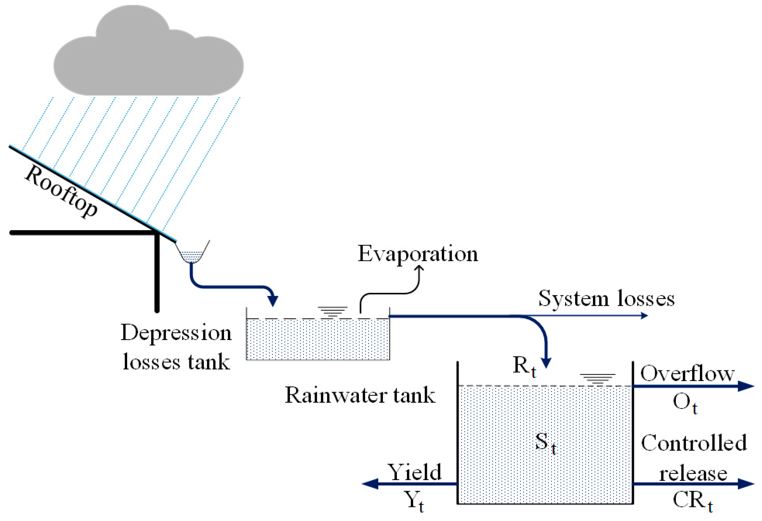
where t is the current timestep; S is volume of water stored in the tank; R is inflow from rainfall; Y is yield or demands satisfied by rainwater; O is overflow; and CR is the controlled release flow of water from the tank (see below “real-time control (RTC)”). The model solves this equation for each timestep. The calculation method of inflows (R_t) and yields (Y_t) usually differentiate models from each other. Inflows are a function of rainfall and collection surface. Rainfall data are unique for each location, and could be used as-is if their attributes (timestep and number of records) is sufficient (e.g., [20]). Rainfall data could also be synthesized [16], or generated stochastically [25].

Yields are a function of water demands and the current volume of water in the tank. Yields could serve both indoor demand (toilet flushing, laundry) [29] and/or irrigation [10].

The algorithm of the presented model is described below, and its flowchart is presented in Figure S1 of the Supplementary Material. The model was coded and run with MATLAB by Mathworks.

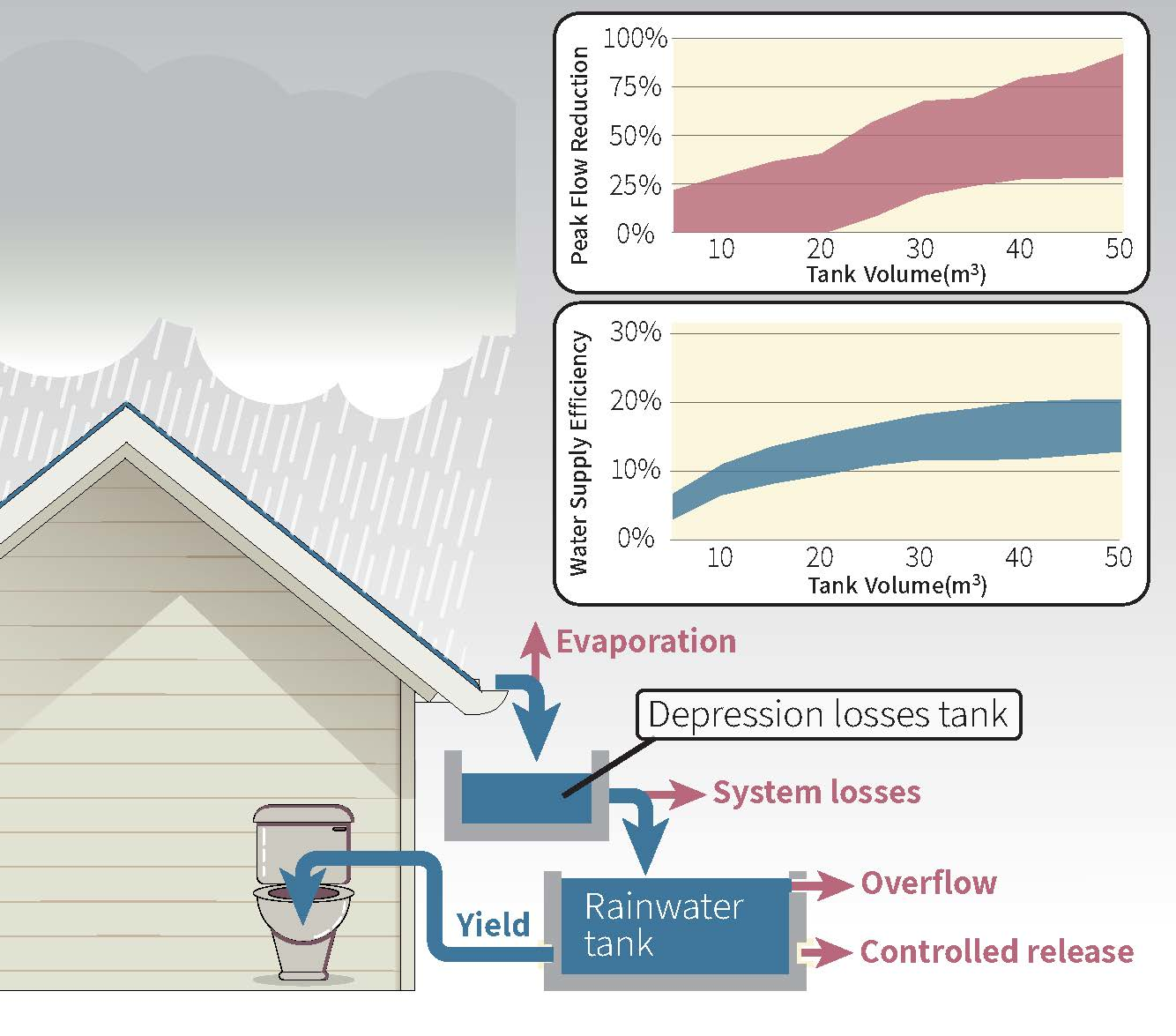
In a timestep with recorded rain, a conceptual depression losses tank fills up (Figure 1). This “tank” simulates the wetting and depression losses of the rooftop. It gains volume by rainfall and loses it by evaporation, both are inputs from the meteorological database. When the depression loses tank is filled, the main rainwater tank begins to receive inflows minus some system loses which represent first flush and leakages from the building’s gutter system. Inflow R_t to the main rainwater tank is given by:

$$R_t=MAX\{\begin{array}{c}0\\ \left(D{L}_{t-1}+D_t-D{L}_{max}\right)\times \left(1-\eta \right)\times A_{roof}\end{array}$$

(2)

where DL is the depression losses tank depth (m); D_t is rain depth (m); DL_max is the maximum depth of the depression losses tank (m); η is gutter system losses (−); and A_roof is the roof area (m²).

The intended use simulated in this study is toilet flushing, as this necessitates minimal treatment (if at all), but other uses (e.g., laundry) can also be simulated. Independently from rainwater fluxes, a demand module creates toilet flushing usage pattern and supplies from the rainwater tank if enough water is available, and partially or fully by potable water otherwise.

The YAS (yield after spillage) approach was chosen as it was found to be more conservative for assessing the water yield for a given storage tank volume [28,30]. According to YAS, if inflows from the roof plus the existing rainwater volume in the tank before demands exceed the capacity of the rainwater tank, overflow occurs. This overflow equals to:

$$O_t=Max\{\begin{array}{c}0\\ S_{t-1}+R_t-S_{max}\end{array}$$

(3)

where S_max is the tank capacity.

When O_t > 0, S_t is set to S_max, and the timestep is completed after demands are fulfilled.

By default, the program simulates full rain seasons (i.e., one simulation run is a run over a full rain season). Nevertheless, the model can simulate any length of rainfall data and could also be used to simulate specific rain events.

The single-building model allows simulations of a customizable number of apartment (and the consequential number of residents) and roof area. For tank design purposes, simulations of different tank sizes for the same building (same roof area and same number of apartments) are available in order to examine the RHW system performance as a function of the storage tank volume.

For long-term performance assessment, it is possible to simulate a succession of randomly selected rain seasons with changing demand patterns, which are derived by a stochastic generator (see below). All the water fluxes presented in Figure 1 were logged to enable any desired post-simulation analysis.

2.2. Efficiency Estimators

To evaluate the RWH system performance for potable water saving and runoff reduction, three efficiency estimators are calculated: water-supply efficiency (WSE), peak-flow reduction (PFR) and overall overflow volume reduction efficiency (VRE).

WSE is the fraction of demands satisfied by rainwater from the overall annual demands. WSE is calculated for each simulated year by summing the yields and demands of all timesteps [10,25]:

$$\mathrm{WSE}=\frac{{\displaystyle \sum }{Y}_t}{{\displaystyle \sum }{d}_t}$$

(4)

where d_t is the is water demand of the designated use (toilet flushing in this study) for timestep t.

PFR is the reduction of the maximum roof runoff per simulated year when RWH is implemented. In other words, PFR compares the maximum flow of water from the roof with and without the RWH system. As it is possible that the RTC module will trigger a controlled release while overflow occurs (see “real-time control”), the sum of both flows for each timestep is taken into consideration when calculating PFR [24]:

$$\mathrm{PFR}=1-\frac{\max \left(O_t+C{R}_t\right)}{\max \left(O_t, S_{max}=0\right)}$$

(5)

where max(O_t + CR_t) is the maximum sum of overflow and controlled release for a specific timestep from the storage tank recorded in a certain year, and max(O_t, S_max = 0) is the maximal recorded overflow for the same year where the tank volume (S_max) is 0, i.e., the maximum roof runoff (with no RWH system).

VRE is the reduction of the annual runoff volume generated from the roof. VRE also quantifies the efficiency of the RWH system for using the available annual rainwater (identical to RUE: rainwater use efficiency in [25]). For example, a VRE of 1 means that all annual rainwater volume was supplied, and none overflowed or were released to the urban drainage system:

$$\mathrm{VRE}=1-\frac{{\displaystyle \sum }(O_t+C{R}_t)}{{\displaystyle \sum }{R}_t}$$

(6)

2.3. Real-Time Control (RTC)

A RTC module was set up based on [20]. The module enables examining different strategies of controlled release from the storage tank: the residual volume of water to be left in the tank is the decision parameter α. The model allows several values to be examined in parallel, from 0 (complete emptying of the tank) to 1 (no intentional water release).

Twice a day, at 12:00 and 24:00, the RTC module obtains a forecast for the total predicted amount of rain for the next 24 h. For the current simulation purposes, it was assumed that the forecast is 100% accurate as it is derived from the rainfall data. It should be noted that this could be changed in the future to allow for uncertainty and errors in rainfall forecasts. Based on this forecast, the module determines whether overflow from the storage tank is predicted during the next 24 h, i.e., the expected rainfall volume (R_t) plus the current volume of water in the tank (S_t) exceed the overall tank volume. If so, the module simulates the opening of a valve (conceptually installed at the bottom part of the tank) for releasing water in a controlled manner. The release flowrate is a function of the current water level in the tank and the orifice’s cross-sectional area:

$$Q_{C{R}_t}=C_d\times A\times \sqrt{2\times g\times h}$$

(7)

where Q_CRt is the controlled release rate of flow, C_d is the coefficient of discharge, A is the orifice’s cross-sectional area, g is the gravitational acceleration and h is the height of water column above the orifice.

The total volume of the released rainwater CR_t is calculated by implementing the numerical midpoint method and multiplying the resulting controlled release flow with the timestep duration.

If inflows are smaller than the controlled release, Q_CR declines with time, as the height of the water above the release valve decreases. To investigate different release policies, a release decision parameter α ranging from 0 to 1 is introduced, and the valve will remain open and release water until the following term is satisfied:

$$S_t\le S_{max}\times \alpha$$

(8)

or until the next forecast predicts no overflow in the following 24 h.

In this manner, high α values mean favoring water supply over runoff mitigation, as more water is kept in the tank and available for supply, but less free volume is available for receiving the roof runoff and preventing overflows from the tank.

2.4. Water Demand

Excluding irrigation, toilet flushing is the most significant non-potable domestic water consumer [31,32]. Toilet flushing demand data was adapted from [33], and includes water demands from 15 households for a period of 3 weeks each. Measurements were taken at 1-s temporal resolution and are classified by water appliance. Data were aggregated to 10-min temporal resolution to fit the timestep of the model. The modeling framework was built under the assumption that Israeli households rarely irrigate during winter (see Section 2.5 below), let alone during and shortly after rain events. As such, demands from the rainwater tank were set to include only toilet flushing.

2.5. Meteorological Data of the Case Study

As one of the goals of the model is to assess RWH effects on urban drainage flows, the model must rely on sub-hourly input data both for inflows (rainfall) and outflows (water demands). The Israeli Meteorological Service’s (IMS) longest recording rain gauge of sub-hourly timesteps is located at Bet Dagan meteorological station at Israel’s central coastal plain (32.0 N, 34.8 E), and could be seen to represent the rainfall patterns of the country’s major urban center. The Israel coastal has a hot-summer-Mediterranean climate (Csa under the Köppen climate classification), with precipitation occurring only from September to May, and mainly from November to March. Summer (June to August) is literally dry. During winter, rain events are sporadic with long dry periods between consecutive events.

The case study weather input includes rainfall measurements of 22 winter seasons from Bet Dagan weather station in 10-min timesteps; 20 consecutive seasons from 1999 until 2019 plus the 1993–1994 and 1994–1995 winters, and the corresponding evaporation data in daily timesteps, with the latter used to simulate wetting loses (see modeling framework above).

Missing records were infilled using neighboring weather stations (if available) or linear interpolation, so that the cumulative 10-min timestep rain depth would sum up to the measured daily rain depth.

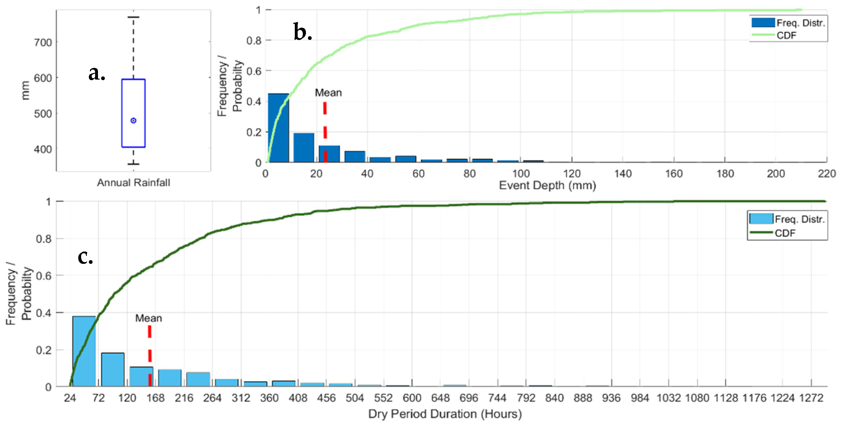
The annual average rainfall of the dataset was 507 mm, slightly below the long-term average of the Bet Dagan station (524 mm). The 25–75 percentiles were 405 and 595 mm, respectively, with median value of 479 mm (Figure 2a). The 22 recorded seasons had, on average 21.5 rain events per season, where a rain event is defined as rainfall of at least 1 mm with 24 h of preceding dry weather. The average rain event in the recorded dataset had 23.5 mm falling in 32.5 h. The average dry period between consecutive rain events (excluding the long dry summer) lasted 160 h, or 6.67 days (Figure 2c).

2.6. Stochastic Modelling Framework

To produce rainfall and demand inputs using the available data, a stochastic approach was taken using sampling with replacement; randomly choosing one dataset for each rain season and for each day of the simulation.

At the beginning of each simulated year, a random dataset representing one rain season (from the meteorological data described above) is selected from the pool of available data. This rain season’s records will be used for the entire simulated year alongside its corresponding evaporation data.

To produce sufficient demand data series in an appropriate temporal resolution at a household-scale, a method of generating stochastic water use patterns was adapted from [34]. Using sampling with the replacement of each apartment in the modeled building enables simulating long time periods with short timesteps, while producing demand patterns which correspond with realistic diurnal patterns of toilet flushing.

Given that most people have daily routines, residential water demand, and toilet flushing in particular follow a diurnal pattern [35,36]. To produce this typical shape while using the available demand data, each apartment of the modeled building was assigned randomly to one of the 15 households from Shteynberg’s measured data [33]. Then, for each modeled apartment, a whole day of toilet flushing demands was drawn randomly at the beginning of each simulated day (00:00 h) from the relevant real-life data. This random drawing was repeated for each apartment at the beginning of each simulated day. In this way, even if the modeled building is larger than 15 apartments (the number of households in the real-life database) and some apartments in the simulated building are assigned the same real-life household, each day of demands of the entire building is different, demands are not degenerated into deterministic values, and the overall diurnal pattern is kept. As the demand patterns on weekdays and weekend days differ, at 00:00 h the model determines whether the upcoming day is weekday or weekend day (Friday or Saturday in Israel) and draws an appropriate day of demands for each apartment.

This manner of drawing datasets ensures the integrity of the data as well as its uniqueness; while each recorded year of rain data is used several times during the simulation, it meets different set of demands each time. The same principle is applied to the smaller loop of drawing demands; the daily demand dataset i for apartment j in Shteynberg’s data is used several times during each simulation for different apartments in the modeled building, but each time it combines with different demand datasets to produce a unique day of demands for the entire modeled building.

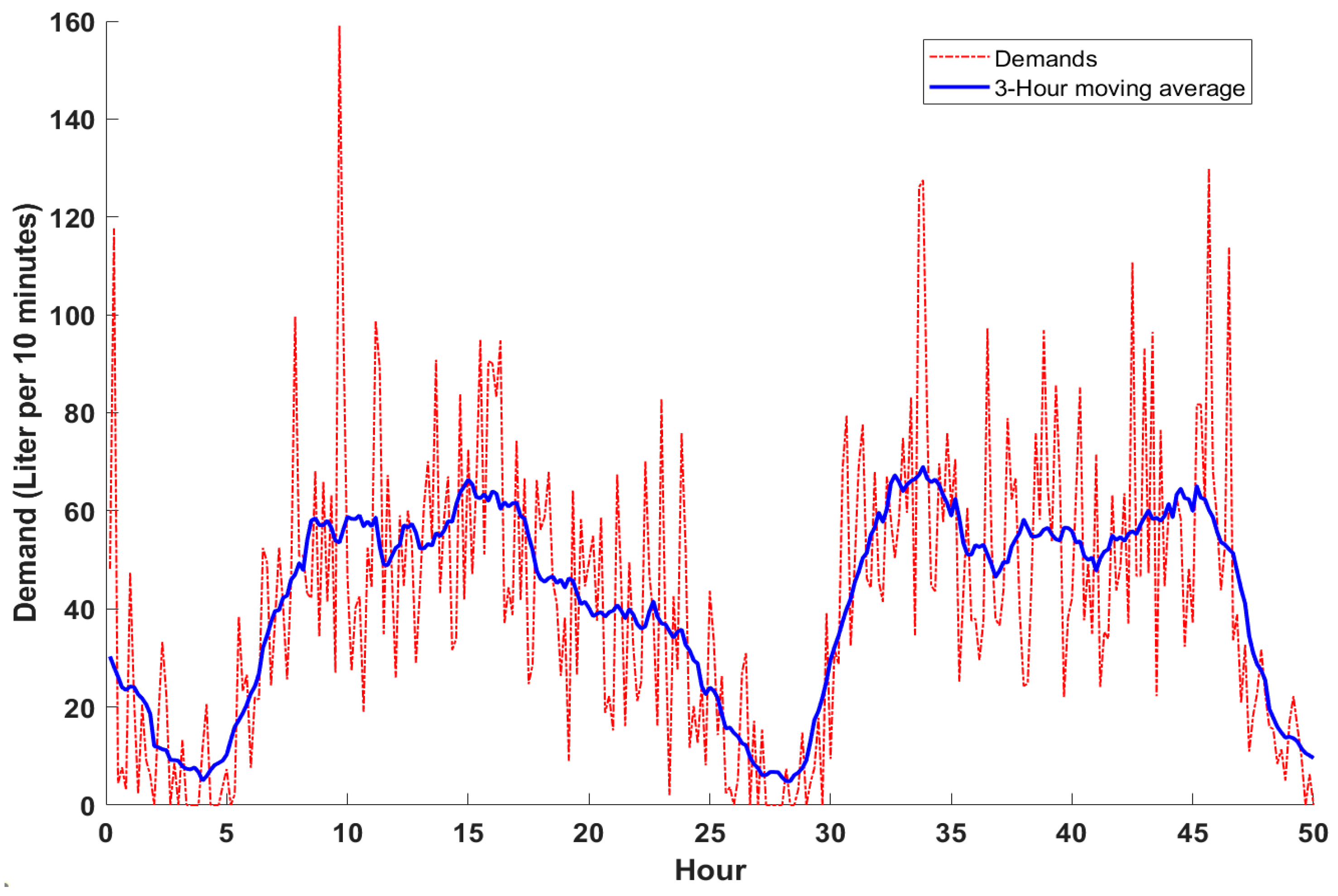
The example of a generated demand pattern for a 40-apartment building is presented in Figure 3. Although the demands for each 10-min timestep are erratic (as would be the case in a real building), smoothing the raw data with a 3-h moving average reveals a typical residential diurnal pattern of toilet flushing [35,36]. The average consumption for toilet flushing is 33 L/(person·d), which corroborates the average value in [36].

3. Results and Discussion

In this section, the model’s output is presented, and possible analyses of the output are demonstrated, including rainwater tank volume examination, creating efficiency curves, and investigating possible controlled release policies (RTC). The parameters used in the simulations are presented in

Table 1. Parameters of the simulated RWH system.

System Losses	Depression Losses	Num of Apts.	Roof Area	Orifice Diameter (RTC)	Simulation Timestep
10%	0.5 mm	40	840 m2	1 cm	10 min

.

3.1. Storage Tank Sizing

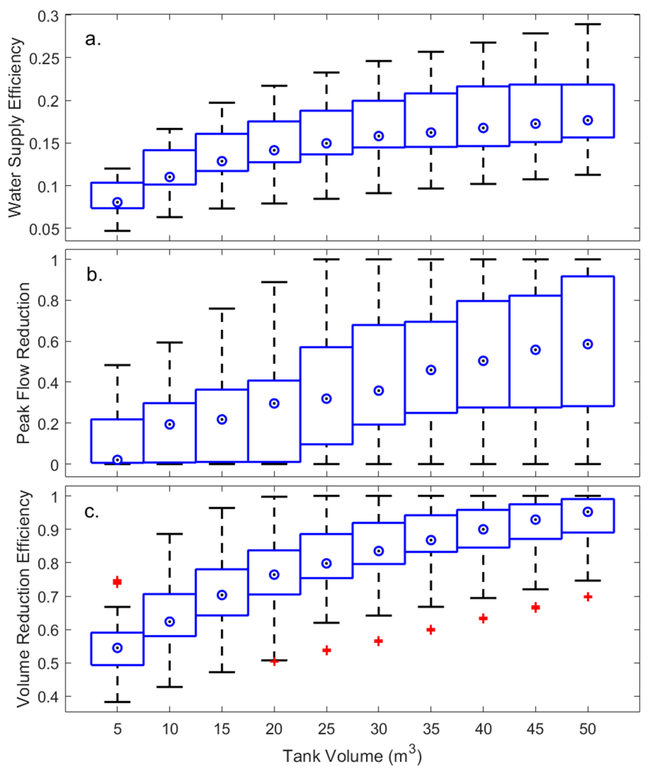
For the simulated building, the WSE (water supply efficiency) demonstrates a logistic growth pattern, showing that increasing the tank size above 30 m³ carries little benefit. PFR (peak-flow reduction) values grow linearly and are scattered along the y axis from 0 to 1. The VRE (volume reduction efficiency) values suggest that a significant portion of the annual rainfall could be harvested and used even with relatively small tanks.

One of the common uses of RWH models is to evaluate different system designs, mainly the sizing of rainwater tanks. The modeling framework allows simulating different tank volumes for the same building and demand patterns. A 40-apartment building with a roof area of 840 m² was modeled. The model was executed for 100 randomly selected rain seasons. WSE, PFR, and VRE were calculated (Figure 4).

Mean annual demands were summed to 1930 m³/year, and the mean annual rainwater volume harvested (i.e., annual rain X roof area minus depression losses minus transfer losses; Equation (2)) was 341 m³. This corresponds with [7], who estimated the annual available rainwater volume from a 850 m² roof in an areas of Jordan with average rainfall of 500 mm per year to be 360 m³.

The WSE shows typical saturation growth curve, with the marginal utility diminishing as the storage tank size increases. For a 50 m³ storage tank, the median WSE reaches 0.18 (25–75 percentiles from 0.16 to 0.22) of the total annual demand (including the rainy winter and the dry summer), which corresponds with the findings of [29] on RWH feasibility in apartment buildings. Another simulation was conducted on a building with 16 apartments with a roof area of 400 m², similar to a building modeled by [25]. The results show similar correlations between WSE and tank volume, with WSE reaching a maximum value of 0.19 with a tank volume of 35 m³ or above. Muklada’s results showed a maximum value of 0.2 for WSE for the same tank volume while also supplying rainwater for laundry. It should be noted that in Muklada’s study demand data were deterministic, and the model was executed on a daily timestep. These differences could have caused the difference in the maximum WSE between the current study and Muklada’s findings.

A building with 16 apartments and a 800 m² roof was simulated to check the model’s correspondence with the findings of Palla et al. [37], who examined the WSE of RWH systems in Catania, Italy (590 mm mean annual rainfall). According to Palla et al. a building with a 50 m³ tank and similar annual rainwater volume to annual demands ratio would reach WSE of 0.4, while the present model estimated a WSE of 0.35. This difference could be explained by the fact that rainfall in Israel characterized by short and intense storms, scattered mainly from November to March. This is causes more frequent overflows and less rainwater availability to satisfy demands. The modeled building with a 50 m³ tank is able to collect 75% of the annual rainwater while the rest overflows, compared with a building with the same attributes in Catania, which is expected to collect more than 90% of the annual rainfall according to Palla et al.

In comparison to the limited growth of WSE values, PFR median values (Figure 4b) increase linearly with increasing modeled storage volume. This difference could be explained by the fact that the annual rainfall is able to supply a limited fraction from the total annual toilet flushing demands. However, it is possible (although probably not economically viable) to install a tank large enough to hold all the annual rainfall and decrease overflow to 0, thus resulting in a PFR value of 1.

Like WSE, VRE shows logistic growth with increasing tank size (Figure 4c). It was demonstrated that even the smallest 5 m³ tank is capable to capture 54% of the annual rainfall. Therefore, 50 m³ tanks can collect 95% (median value, 25–75 percentiles from 89% to 99%) of the annual rainfall, and all tank sizes larger than 25 m³ enable the use of at least 80% (median value) of the annual rainfall, or in other words, an at least 80% reduction of the annual overflow volume.

3.2. Efficiency Curves

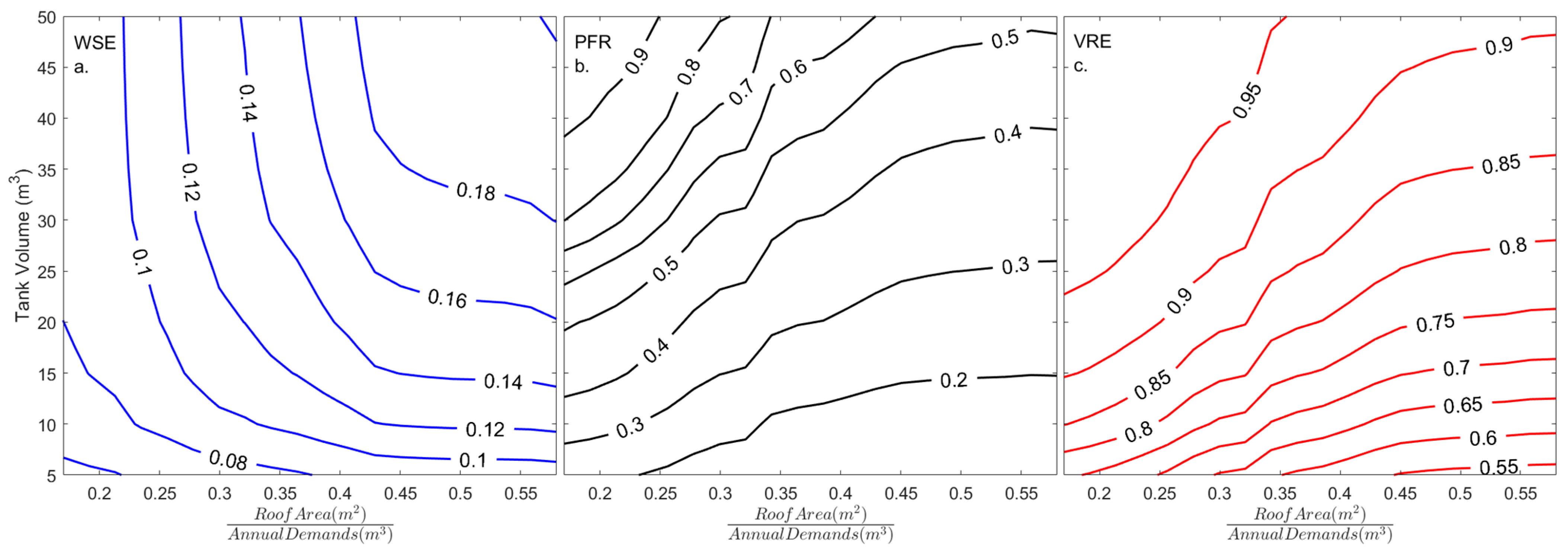
Another possible use of the model is to create efficiency curves for expected WSE, PFR and VRE as was suggested by [38] and adapted by [39]. These curves enable the assessment of the efficiency estimators’ values for a wide range of buildings, and examining the effects of different tank designs in an accessible manner. For the efficiency curves presented here, 100 different apartment buildings with roof areas of 400 to 900 m² and an apartment number of 30–60 were modelled under similar 100 rain-season simulation, resulting in 100 PFR, WSE and VRE results per building. Contour plots of the mean values of the estimators were charted as a function of storage tank volume and the normalized roof area (roof area (m²) divided by mean annual demands (m³); Figure 5).

These curves can be used to estimate the benefit of installing RWH systems in different buildings. To demonstrate this, let our designated building be the abovementioned 40-apartment building with a roof area of 840 m², and an estimated annual toilet flushing water use of 1930 m³ (the latter can be estimated by multiplying the number of tenants by the expected annual water use for toilet flushing per capita). This building has a roof area to annual demand ratio of 0.45 m⁻¹. For the purpose of this demonstration, the main objective of installing the RWH system in this building is to reduce the expected peak flow from the roof by 40%. By examining the PFR curves, it can be deducted that a rainwater tank of 35 m³ would reduce the annual peak flows by 40% (on average) and would be able to supply about 17% of the annual toilet flushing water demand (WSE). If the desired PFR is 0.5, a tank of 45 m³ would be needed for the same building. A tank of such volume would supply 18% of the annual demand for toilet-flushing, and reduce by 90% the annual overflow volume (VRE) of the system.

3.3. RTC Policies

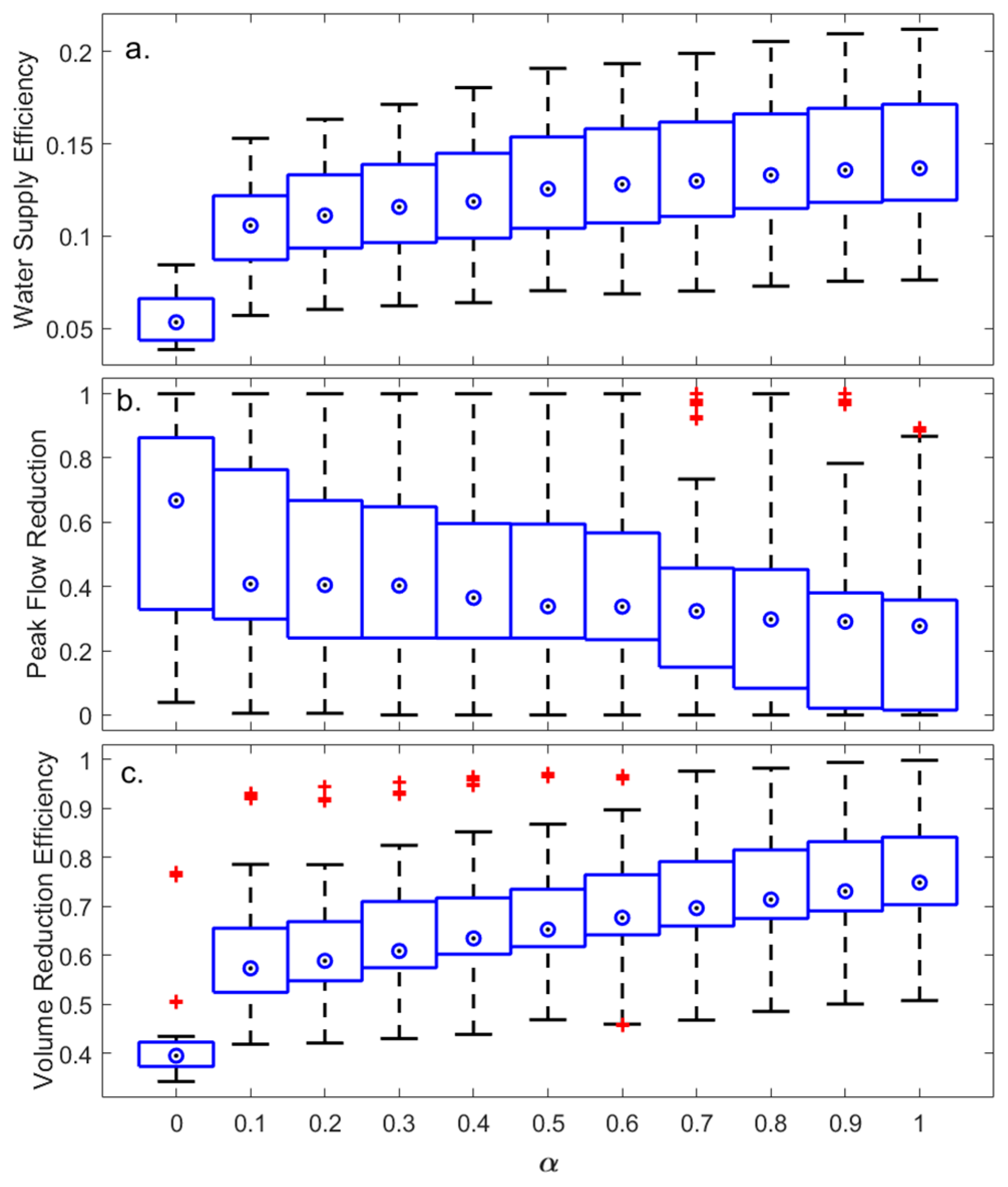
Except for a policy of completely emptying the storage tank prior to expected overflows, applying RTC improves PFR significantly with minor impacts on WSE.

For the same 40-apartment building and simulation parameters used for tank design purposes, different values of release decision parameter α were examined (see Section 2.3 above)for a 20 m³ tank. The simulation included 100 years, and a total of 11 systems were simulated. Each RWH system was modelled with similar rain seasons and supplied water to the same building with identical demands, with the only difference being the value of α (α = 0, 0.1, 0.2,…, 1).

The results show that setting α to 0, meaning complete discharge of stored water prior to a storm where overflow is predicted to occur, carries significant impact for the WSE, with only 5% of demands (median value) satisfied by rainwater (Figure 6a). Slightly increasing α to 0.1 (water is released from the tank until storage is 10% of the full tank capacity) more than doubled the supply efficiency to 11% (median value). For an α between 0.1 and 1, the median values of WSE increase linearly with α, peaking at 14% of demands when α = 1; no water is released prior to rain events.

In comparison, after a significant decrease of the median PFR (39% decrease) when increasing α from 0 to 0.1 (from 0.67 to 0.41), there is only a 32% drop in PFR values when α increases from 0.1 to 1 (the maximum possible value), where the PFR median is 0.28. This phenomenon could be explained by the fact that PFR refers to the maximum values of overflow for a simulated year, which are a result of one specific maximal rain event per rain season that cannot be contained other than by complete discharge of the tank.

Setting α to 0 significantly diminishes the system’s rainfall use efficiency, as the VRE drops to 0.4, meaning that only 40% of the available water is used while 60% is released or overflows to the urban drainage system as the tank is fully emptied when overflow is expected. Increasing α to only 0.1 is enough to raise VRE substantially, to 0.57 (median value), and a further increase in α results in linear growth of VRE up to 0.75, with no controlled release (α = 1).

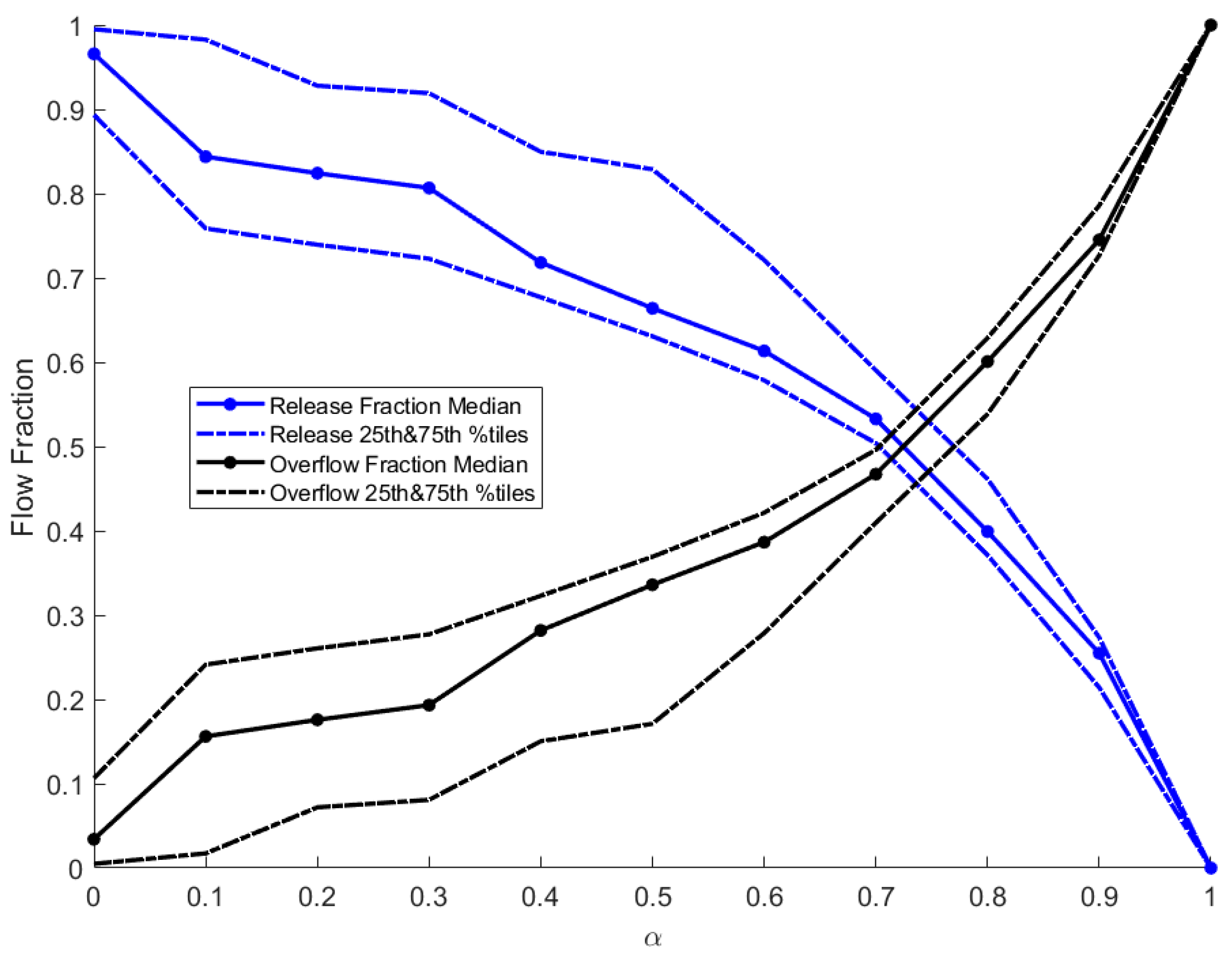
As VRE accounts for water losses due to overflows and controlled release, further examination of these flows was conducted. For each value of α, each loss (overflows and controlled release) was summed annually and the fraction of each from the total water losses (overflows plus controlled releases) was calculated. To achieve this the simulation was executed for the 40-apartment building with a RWH tank of 20 m³ and run for 100 years (as before).

For the simulated building, equilibrium (i.e., equal overflow and controlled release volumes, Figure 7) was observed at α values of 0.7–0.8, where the median values of VRE, PRF and WSE were 0.7, 0.3, and 0.13, respectively. When α = 1 the VRE, PFR and WSE medians were 0.75, 0.28 and 0.14 respectively. When α is reduced to 0.5, 65% of the total water losses are through controlled release, while 35% is through overflow (median values), and the median values of WSE, PFR and VRE are 0.13, 0.34 and 0.65, respectively.

In general, when excluding the complete discharge policy (α = 0), PFR is more sensitive than WSE to changes in α. When reducing α from 1 (no controlled release) to 0.1, the WSE median drops by 23% from 0.137 to 0.106, while PFR increases by 48%, from 0.276 to 0.408. This difference in sensitivity is further enhanced when examining a mid-range α value. For example, when applying RTC and setting α = 0.3, the PFR median value increases by 45% in comparison to α = 1 (no controlled release) from 0.275 to 0.4, respectively. Under this RTC policy, the WSE median value decreases by 15% (from 0.137 to 0.116). When considering that the mean annual demands for the modeled building are 1930 m³/year, this decrease reduces the total volume of supplied rainwater by 40 m³. When setting α = 0.3, the VRE median value decreases by 19% (from 0.75 to 0.61).

These findings correspond with those of [20], who found that implementing controlled release could have significant effects on PFR, with minor impact on WSE, and estimated a decrease of 10% in WSE when using a real-time controlled orifice to handle overflows from rainwater tanks. Such results from applying a simple RTC policy suggest that more sophisticated policies should be explored as they can potentially yield even better dual objectives performance of RWH systems for reducing potable water demand and minimizing overflows to urban drainage systems.

4. Conclusions

A high-temporal resolution stochastic RWH model aimed at assessing potable water savings and runoff reduction was developed using real-life water demand and rainfall data. The presented model does not include tank size optimization, as such process requires a cost–benefit analysis which was beyond the scope of this study. Such a cost benefit analysis addressing the dual benefit of RWH, supplying water while reducing drainage flows, is expected to be site specific with a high dependency on the characteristics of the local drainage system and the urban watershed.

Model attributes include:

• The model enables simulation of various buildings (varying in the number of apartments and dwellers), collection surface (roof) areas, rainwater tank volumes and time periods; from single rain events up to multi-seasonal simulations
• Model inputs (rainfall and demands) are used in a stochastic manner (sampling with replacement), which maintains their natural pattern while generating realistic noise and temporal variability. In this way, creating rainfall and demand data series does not require rigorous data analysis on the one hand, and does not degenerate input data to constant or deterministic values on the other.

The model could be used for:

• Estimating the short term benefits such as runoff reduction for specific storms, as well as long term evaluations of peak runoff flow reduction, overall annual overflow volume reduction, and rainwater supply efficiencies.
• Comparing the performances of different tank sizes under the same conditions
• Drawing design curves for a range of tank sizes and roof areas for specific rainfall data
• Inspecting different RTC policies and their effects on the system’s efficiency.

This modeling framework can serve as the basis for studying the effects of RWH on urban drainage, as it could be easily adjusted to simulate different buildings or residential clusters. The influences of different system design, spatial distributions of the rainwater tanks, or different and more elaborate controlled release policies could be estimated when the suggested model is coupled with a drainage model of the desired urban watershed. Future work will include developing such combined RWH harvesting—Drainage models for several case studies, where overflows from the presented framework will serve as part of the input for the drainage models.

References

- Campisano, A.; Butler, D.; Ward, S.; Burns, M.J.; Friedler, E.; DeBusk, K.; Fisher-Jeffes, L.N.; Ghisi, E.; Rahman, A.; Furumai, H.; et al. Urban Rainwater Harvesting Systems: Research, Implementation and Future Perspectives. Water Res. 2017, 115, 195–209. [Google Scholar] [CrossRef] [PubMed]
- Ranaee, E.; Abbasi, A.A.; Yazdi, J.T.; Ziyaee, M. Feasibility of Rainwater Harvesting and Consumption in a Middle Eastern Semiarid Urban Area. Water 2021, 13, 2130. [Google Scholar] [CrossRef]
- Farreny, R.; Morales-Pinzón, T.; Guisasola, A.; Tayà, C.; Rieradevall, J.; Gabarrell, X. Roof Selection for Rainwater Harvesting: Quantity and Quality Assessments in Spain. Water Res. 2011, 45, 3245–3254. [Google Scholar] [CrossRef] [PubMed]
- Rahman, A. Recent Advances in Modelling and Implementation of Rainwater Harvesting Systems towards Sustainable Development. Water 2017, 8, 959. [Google Scholar] [CrossRef] [Green Version]
- Campisano, A.; Modica, C. Optimal Sizing of Storage Tanks for Domestic Rainwater Harvesting in Sicily. Resour. Conserv. Recycl. 2012, 63, 9–16. [Google Scholar] [CrossRef]
- Semaan, M.; Day, S.D.; Garvin, M.; Ramakrishnan, N.; Pearce, A. Optimal Sizing of Rainwater Harvesting Systems for Domestic Water Usages: A Systematic Literature Review. Resour. Conserv. Recycl. X 2020, 6, 100033. [Google Scholar] [CrossRef]
- Abdulla, F. Rainwater Harvesting in Jordan: Potential Water Saving, Optimal Tank Sizing and Economic Analysis. Urban Water J. 2020, 17, 446–456. [Google Scholar] [CrossRef]
- Domínguez, I.; Ward, S.; Mendoza, J.G.; Rincón, C.I.; Oviedo-Ocaña, E.R. End-User Cost-Benefit Prioritization for Selecting Rainwater Harvesting and Greywater Reuse in Social Housing. Water 2017, 9, 516. [Google Scholar] [CrossRef] [Green Version]
- Dallman, S.; Chaudhry, A.M.; Muleta, M.K.; Lee, J. Is Rainwater Harvesting Worthwhile? A Benefit–Cost Analysis. J. Water Resour. Plan. Manag. 2021, 147, 04021011. [Google Scholar] [CrossRef]
- Steffen, J.; Jensen, M.; Pomeroy, C.A.; Burian, S.J. Water Supply and Stormwater Management Benefits of Residential Rainwater Harvesting in U.S. Cities. J. Am. Water Resour. Assoc. 2013, 49, 810–824. [Google Scholar] [CrossRef]
- Freni, G.; Liuzzo, L. Effectiveness of Rainwater Harvesting Systems for Flood Reduction in Residential Urban Areas. Water 2019, 11, 1389. [Google Scholar] [CrossRef] [Green Version]
- Vaes, G.; Berlamont, J. The Effect of Rainwater Storage Tanks on Design Storms. Urban Water 2001, 3, 303–307. [Google Scholar] [CrossRef]
- United States Environmental Protection Greening CSO Plans: Planning and Modeling Green Infrastructure for Combined Sewer Overflow (CSO) Control U.S. Environmental Protection Agency. 2014. Available online: https://www.epa.gov/sites/production/files/2015-10/documents/greening_cso_plans_0.pdf (accessed on 20 January 2021).
- Campisano, A.; Modica, C. Selecting Time Scale Resolution to Evaluate Water Saving and Retention Potential of Rainwater Harvesting Tanks. Procedia Eng. 2014, 70, 218–227. [Google Scholar] [CrossRef] [Green Version]
- Palla, A.; Gnecco, I.; La Barbera, P. The Impact of Domestic Rainwater Harvesting Systems in Storm Water Runoff Mitigation at the Urban Block Scale. J. Environ. Manag. 2017, 191, 297–305. [Google Scholar] [CrossRef] [PubMed]
- Quinn, R.; Rougé, C.; Stovin, V. Quantifying the Performance of Dual-Use Rainwater Harvesting Systems. Water Res. X 2021, 10. [Google Scholar] [CrossRef] [PubMed]
- Burns, M.J.; Fletcher, T.D.; Duncan, H.P.; Hatt, B.E.; Ladson, A.R.; Walsh, C.J. The Performance of Rainwater Tanks for Stormwater Retention and Water Supply at the Household Scale: An Empirical Study. Hydrol. Process. 2015, 29, 152–160. [Google Scholar] [CrossRef]
- Gee, K.D.; Hunt, W.F. Enhancing Stormwater Management Benefits of Rainwater Harvesting via Innovative Technologies. J. Environ. Eng. 2016, 142, 04016039. [Google Scholar] [CrossRef]
- Oberaschermsn, M.; Rauch, W.; Sitzenfrei, R. Efficient Integration of LoT-Based Micro Storages to Improve Urban Drainage Performance through Advanced Control Strategies. Water Sci. Technol. 2021, 83, 2678–2690. [Google Scholar] [CrossRef] [PubMed]
- Xu, W.D.; Fletcher, T.D.; Duncan, H.P.; Bergmann, D.J.; Breman, J.; Burns, M.J. Improving the Multi-Objective Performance of Rainwater Harvesting Systems Using Real-Time Control Technology. Water 2018, 10, 147. [Google Scholar] [CrossRef] [Green Version]
- Di Matteo, M.; Liang, R.; Maier, H.R.; Thyer, M.A.; Simpson, A.R.; Dandy, G.C.; Ernst, B. Controlling Rainwater Storage as a System: An Opportunity to Reduce Urban Flood Peaks for Rare, Long Duration Storms. Environ. Model. Softw. 2019, 111, 34–41. [Google Scholar] [CrossRef]
- Labadie, J.W. Optimal Operation of Multireservoir Systems: State-of-the-Art Review. J. Water Resour. Plan. Manag. 2004, 130, 93–111. [Google Scholar] [CrossRef]
- Zhang, J.; Cai, X.; Lei, X.; Liu, P.; Wang, H. Real-Time Reservoir Flood Control Operation Enhanced by Data Assimilation. J. Hydrol. 2021, 598, 126426. [Google Scholar] [CrossRef]
- Liang, R.; Thyer, M.A.; Maier, H.R.; Dandy, G.C.; Di Matteo, M. Optimising the Design and Real-Time Operation of Systems of Distributed Stormwater Storages to Reduce Urban Flooding at the Catchment Scale. J. Hydrol. 2021, 602, 126787. [Google Scholar] [CrossRef]
- Muklada, H.; Gilboa, Y.; Friedler, E. Stochastic Modelling of the Hydraulic Performance of an Onsite Rainwater Harvesting System in Mediterranean Climate. Water Sci. Technol. Water Supply 2016, 16, 1614–1623. [Google Scholar] [CrossRef] [Green Version]
- Nachshon, U.; Netzer, L.; Livshitz, Y. Land Cover Properties and Rain Water Harvesting in Urban Environments. Sustain. Cities Soc. 2016, 27, 398–406. [Google Scholar] [CrossRef]
- Abdulla, F.A.; Al-Shareef, A.W. Roof Rainwater Harvesting Systems for Household Water Supply in Jordan. Desalination 2009, 243, 195–207. [Google Scholar] [CrossRef]
- Fewkes, A. Modelling the Performance of Rainwater Collection Systems: Towards a Generalised Approach. Urban Water 2000, 1, 323–333. [Google Scholar] [CrossRef]
- Morales-Pinzón, T.; Rieradevall, J.; Gasol, C.M.; Gabarrell, X. Modelling for Economic Cost and Environmental Analysis of Rainwater Harvesting Systems. J. Clean. Prod. 2015. [Google Scholar] [CrossRef]
- Mitchell, V.G. How Important Is the Selection of Computational Analysis Method to the Accuracy of Rainwater Tank Behaviour Modelling? Hydrol. Process. 2007, 21, 2850–2861. [Google Scholar] [CrossRef]
- Butler, D.; Friedler, E.; Gatt, K. Characterising the Quantity and Quality of Domestic Wastewater Inflows. Water Sci. Technol. 1995, 31, 13–24. [Google Scholar] [CrossRef]
- Friedler, E. The Water Saving Potential and the Socio-Economic Feasibility of Greywater Reuse within the Urban Sector—Israel as a Case Study. Int. J. Environ. Stud. 2008, 65, 57–69. [Google Scholar] [CrossRef]
- Shteynberg, D. Measurement and Simulation of the Diurnal Pattern of Domestic Water Demand on Micro-Component Scale. Master’s Thesis, Technion—Israel Institute of Technology, Haifa, Israel, 2015. Available online: https://www.graduate.technion.ac.il/Theses/Abstracts.asp?Id=29200 (accessed on 24 March 2021).
- Penn, R.; Schütze, M.; Gorfine, M.; Friedler, E. Simulation Method for Stochastic Generation of Domestic Wastewater Discharges and the Effect of Greywater Reuse on Gross Solid Transport. Urban Water J. 2017, 14, 846–852. [Google Scholar] [CrossRef]
- Friedler, E.; Butler, D.; Brown, D.M. Domestic WC Usage Patterns. Build. Environ. 1996, 31, 385–392. [Google Scholar] [CrossRef]
- Mayer, P.; DeOreo, W.B. Residential End Uses of Uses Water; AWWA Research Foundation: Denver, CO, USA, 1999; pp. 125–132. ISBN 978-1-58321-016-1. [Google Scholar]
- Palla, A.; Gnecco, I.; Lanza, L.G. Non-Dimensional Design Parameters and Performance Assessment of Rainwater Harvesting Systems. J. Hydrol. 2011, 392, 65–76. [Google Scholar] [CrossRef]
- Basinger, M.; Montalto, F.; Lall, U. A Rainwater Harvesting System Reliability Model Based on Nonparametric Stochastic Rainfall Generator. J. Hydrol. 2010, 392, 105–118. [Google Scholar] [CrossRef]
- Rahman, A.; Snook, C.; Haque, M.M.; Hajani, E. Use of Design Curves in the Implementation of a Rainwater Harvesting System. J. Clean. Prod. 2020, 261, 121292. [Google Scholar] [CrossRef]
Figure 1.
Modeling framework of a rainwater harvesting system. The conceptual depression losses tank needs to overflow to initiate inflows to the main rainwater tank. The rainwater tank is gaining water when Rt > 0, and lose water due to overflows, yield (demands) or controlled release (if the latter is modeled).
Figure 2.
Rainfall data from Bet Dagan (Israel) meteorological station (a) Box plot of annual rainfall. (b) Frequency distribution and empirical cumulative distribution function (CDF) of rain events depth. (c) Frequency distribution and empirical CDF of dry periods (within the rainy season).
Figure 3.
Two days of toilet flushing demands for 40 apartments created by the stochastic water demand generator. Demands as liter for 10 min (dashed red) show erratic pattern, 3-h moving average reveal typical diurnal pattern.
Figure 4.
WSE PFR and VRE as a function of rainwater tank volume for the modeled building. Median values are marked as circles, boxes represent 25th and 75th percentiles, and whiskers 10th and 90th percentiles. Outliers are marked as red crosses. (a) WSE, (b) PFR, (c) VRE.
Figure 5.
WSE PFR and VRE as a function of normalized roof area (roof area divided by annual demands), and rainwater tank volume. Contours represent constant WSE (a), PFR (b) and VRE (c) values.
Figure 6.
WSE, PFR, and VRE as a function of release parameter, α, for the modeled building with a 20 m3 tank. WSE and VRE decline as more water is released from the tank (smaller α), while PFR increases as more storage is available for incoming roof runoff. (a) WSE, (b) PFR, (c) VRE.
Figure 7.
Overflow and controlled release as fractions of the total loss flow (overflows + controlled release). As more water is released from the tank, the fraction of the released water from the overall outflows increases.