
CFD Model of the Density-Driven Bidirectional Flows through the West Crack Breach in the Great Salt Lake Causeway


1
Department of Civil and Environmental Engineering, Utah Water Research Laboratory, Utah State University, Logan, UT 84322-8200, USA
2
Department of Mechanical and Aerospace Engineering, Utah State University, Logan, UT 84322-8200, USA
*
Authors to whom correspondence should be addressed.
Water 2021, 13(17), 2423; https://doi.org/10.3390/w13172423
Submission received: 1 July 2021
/
Revised: 18 August 2021
/
Accepted: 25 August 2021
/
Published: 3 September 2021
(This article belongs to the Special Issue Numerical Modeling on Hydraulic Structures Flow Associated with Urban and Environmental Engineering)
Abstract
:Stratified flows and the resulting density-driven currents occur in the natural environment and commonly in saline lakes. In the Great Salt Lake, Utah, USA, the northern and southern portions of the lake are divided by an east-to-west railroad causeway that disrupts natural lake currents and significantly increases salt concentrations in the northern section. To support management efforts focused on addressing rising environmental and economic concerns associated with varied saltwater densities throughout the lake, the causeway was recently modified to include a new breach. The purpose of this new breach is to enhance salt exchange between the northern and southern sections of the lake. Since construction, it typically exhibits a strong density-driven bidirectional flow pattern, but estimating flows and salt exchange has proven to be difficult. To obtain much needed insights into the ability of this hydraulic structure to exchange water and salt between the two sections of the lake, a field campaign coupled with CFD modeling was undertaken. Results from this study indicate that the vertical velocity profile in the breach is sensitive to density differences between flow layers along with breach geometry and water surface elevations. The CFD model was able to accurately represent the bidirectional flows through the breach and provides for improved estimates of water and salt exchanges between the north and south sections of the lake.
1. Introduction
Saline lakes represent 23 percent by area, and 44 percent by volume, of all lakes on Earth [1]. Saline lakes can be found in diverse environments, though most of them are terminal lakes and located in places with an arid climate. Some of the major saline lakes are the Caspian Sea (coastline shared by Azerbaijan, Iran, Kazakhstan, Russia, and Turkmenistan), the Great Salt Lake (GSL) (Unites States), and Lake Urmia (Iran). The importance of these lakes is indicated by their proximity to urban centers (e.g., GSL is near Salt Lake City) and their thriving shipping, fishing, mineral, and tourism industries. In addition to direct economic benefits, saline lakes and the surrounding wetlands provide unique habitats for birds and other fauna [2,3]. Climate-change propelled droughts and increases in human consumption have resulted in lowering water levels and volumes of these saline lakes across the world [4]. One of the first recorded incidences of human consumption leading to saline lake desiccation occurred in the Tarim Basin, leading to the downfall of the Loulon Kingdom in 645 CE [5]. Some examples of saline lake desiccation due to over consumption in the last 100 years include Lake Urmia in Iran [6] and Owens Lake in the United States that was entirely dried up in 1940. Desiccation of saline lakes and the resulting alarming decline in related ecosystems have been documented in the past [4,7,8]; this has led to a renewed interest in preserving these systems as a subset of these lakes have seen calamitous decline in lake levels in the last 20 years [9]. The GSL is facing similar issues with the lowest levels being recorded in summer 2021 due to over consumption throughout the watershed. Potential desiccation and related ecosystem issues have been recently highlighted and are a major concern [4].
As the saline lake levels drop due to climate change and over consumption, there is a clear need to understand changes in water and salt transport throughout these lakes. This is of even greater importance where impoundments or structures alter or restrict lake water and salt movement. For example, in the GSL a railroad causeway divides the lake into northern and southern sections and limited connectivity is provided at causeway breaches. In these settings, the water and salt exchanges through these hydraulic structures are difficult to quantify, but critical for management efforts related to long-term ecosystem health and related industries via the evolution of the GSL’s density profile [10,11].
To provide insight regarding the water and salt exchanges needed for GSL management efforts, a field campaign coupled with a computational fluid dynamics (CFD) modeling of the density-driven flows through the recently commissioned West Crack (WC) Breach was undertaken. The modeling effort provides a better understanding of the bidirectional buoyancy-driven flow through the WC breach that provides GSL management and stakeholders with insights into how the openings in the causeway could be used for effective brine management in the future [12,13].
2. Great Salt Lake and the West Crack Breach
The GSL is a significant resource to Utah, contributing more than $1.3 billion annually to Utah’s economy through mineral extraction and its world-leading brine shrimp production [14,15]. Recreational attractions connected to the GSL also play a significant part in the local economy, primarily due to the GSL’s unique ecosystem that provides habitat for almost five million migratory birds every year [16]. As a result, significant research and monitoring efforts have been undertaken for decades [17], especially since the construction of the Union Pacific Railroad Company (UPRR) causeway in 1959. This railroad causeway divides approximately 1/3 of the lake from the southern section (see Figure 1) and has altered its characteristics including natural circulation and the water and salt balances [18]. For example, since 1959 the northern part of the GSL has become more saline while the salt content of the southern part with significant freshwater inflows has reduced [17,19]. The density, ρ, of North saltwaterhas on-an-average been ~100 to 150 kg/m3 higher than the South from 1966 to 2019, except during high lake levels [20]. Two culverts were built in the causeway in 1959 to facilitate water connectivity between the northern and southern sections. Subsequently, a breach was created in 1984 near the western end of the causeway. The original culverts were decommissioned in December 2013 with a second WC Breach (see Figure 2) opened in December 2016. Over the past 3 years, the water surface elevation (WSE) of the northern section of the lake has dropped significantly, illustrating the importance of the flow though the breach on both water and salt balances of the different sections of the GSL.
The difference in density, primarily due to varied salt concentrations, between the northern and southern sections of the GSL results in the formation of density-difference driven flow through the WC breach. In general, the WSE of the southern section is always higher than the north section. If there was no difference in density between the two sides, the flow through the breach would consistently be from South to North. However, the higher density on the North results in south water floating over the north water and the north water plunging in order to flow south. The result is bidirectional flow through the breach, where in the upper portion of the water column typically flows northward and the lower portion, with higher density, flows south. Consequently, this flow results in formation of a stable and stratified, but hydraulically complex, deep brine layer (DBL) in the southern part of the GSL. The connection between the density gradient-driven gravity current flowing through the breach and the formation of DBL is succinctly illustrated by the disappearance of the DBL during a three-year period when the last culvert was closed in December 2013 and a new breach was opened in December 2016 [22]. Although the DBL may be influenced by other factors, analyses had shown strong sensitivity of deeper salinity concentrations in the southern section of the GSL to the geometry and adjacent submerged berms of the new breach [12,13]. This essentially points to the fact that the new WC Breach is the location where most of the exchange of water and salt occurs between the northern and southern section of the lake. Thus, to correctly estimate the water and salt mass balance between two parts of the lake it is imperative to model the flow and salt transport through the WC Breach accurately.
Prior to the WC Breach several modeling efforts were undertaken. One of the first dedicated hydraulics models built to estimate the flow going through the culverts in the causeway was developed by Holley and Waddell [23], and later advanced by Loving et al. [10] to estimate the GSL saltwater densities and bidirectional flow through the causeway. While this model is capable of calculating the bidirectional flow through the causeway openings, the calculated flows were not in good agreement with measured flows, especially with the creation of the new WC breach. This is not completely unexpected due to the fact that Holley and Waddell’s model was developed for bidirectional flow through culverts, which are significantly different geometrically from the bridge built over the breach (see Figure 2). The newer breach has components (e.g., piers) that are expected to make the flow highly three-dimensional (3D). Thus, the complex bidirectional flow though the WC breach warranted the use of a CFD modeling approach to accurately capture the dynamics. In spite of the flow in the GSL being highly three-dimensional and complex, there has been very few studies that have used 3D hydrodynamic modeling to study different aspects of the lake. Spall [24,25] used 3D hydrodynamic models that incorporated baroclinic and barotropic responses, tidal forcing, wind stresses, Coriolis effects, surface thermal forcing, inflows, outflows, and transport of salt, heat, and passive scalars. Spall investigated the effects of surface heat flux and wind forcing on the spatio-temporal variations in the flow patterns within the southern section of the GSL. Neither of the studies modeled the spatio-temporal dynamics of the DBL in the GSL or the bidirectional flow passing through the causeway openings. To address these modeling gaps, a CFD model is required that captures the complex interaction between the bidirectional flow and the hydraulic structure that uses a multiphase CFD solver that can track the interface (fluid–fluid or fluid–air) between different phases. These solvers have been used successfully to study density flows and various complex multiphase flow problems (e.g., multiphase sewage flows in water reclamation plants [26] or estimation of flow discharge through hydraulic structures [27]).
3. Materials and Methods
3.1. Field Campaign
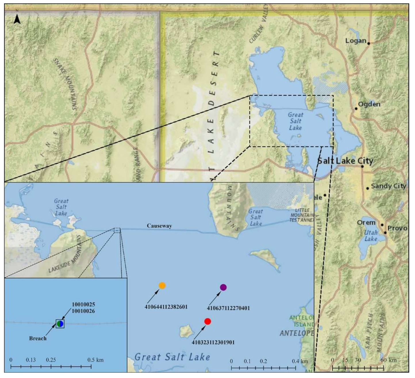
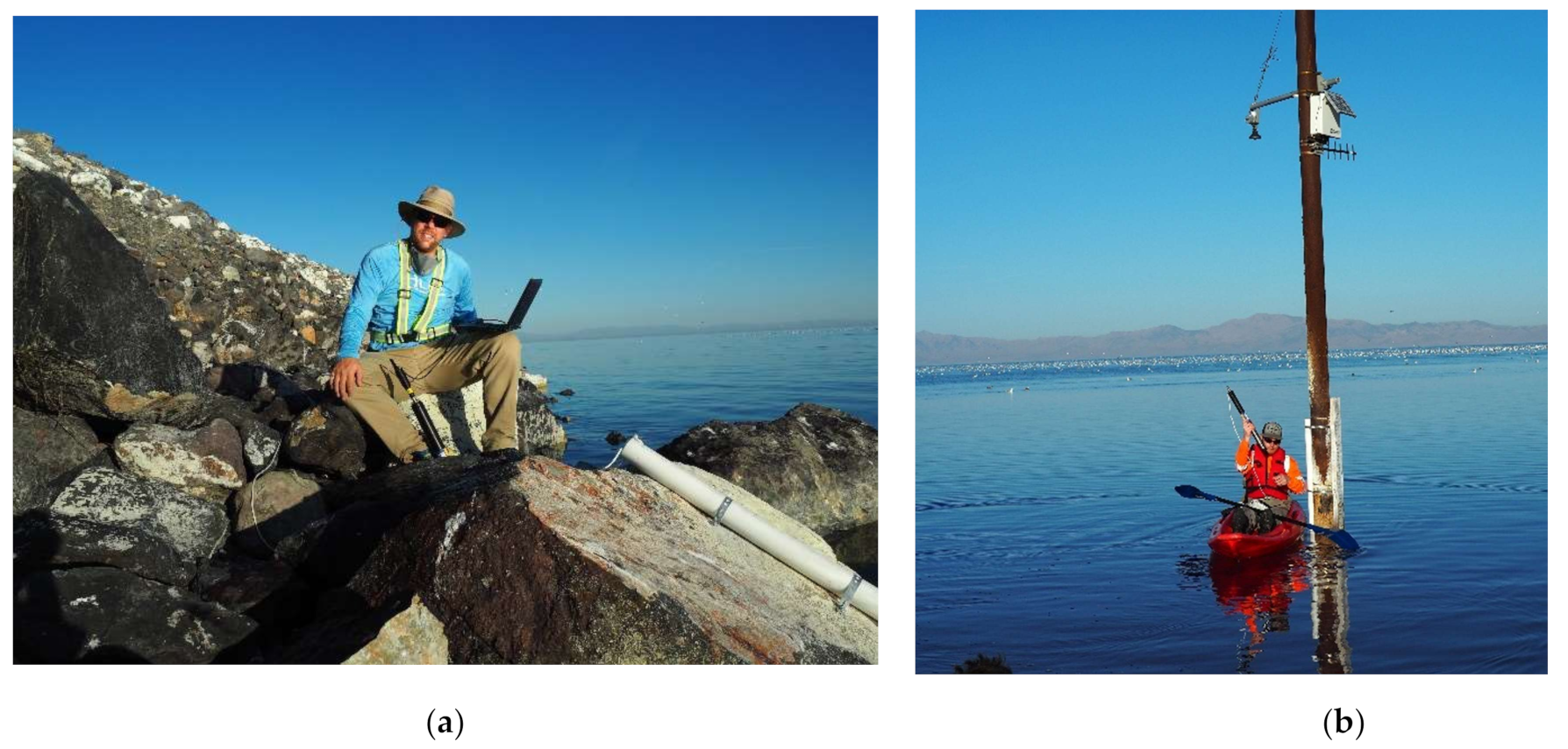
Field measurements were conducted at the WC Breach of the Great Salt Lake causeway, located approximately 53 km northwest of Salt Lake City and about 27 km west of Promontory Point. At this location lake depths were on average less than about 6 m. Field data were collected from 1 October 2020, to June of 2021 with supplemental data obtained from the U.S. Geologic Survey (USGS). USGS field data have been collected from the time the WC Breach was completed (Dec. 2016). Field observations were made as part of this modelling effort via shore access and by kayak (see Figure 3) that focused on specific conductance (σ), total dissolved solids (TDS), and water temperature measurements at and adjacent to the breach.
To better understand the relationship between σ, TDS, and ρ, water samples were collected at multiple locations north and south of the breach at specific flow depths (e.g., 0.1 m to 4.6 m at approximately 0.3 m spacing). Locations were GPS located and depths were measured with a field tape accurate to ±30 mm. A simple tubing and syringe system was used to collect samples, with the tubing placed at the prescribed depth and then a volume secured in the large syringe. Flushing was performed between each sample to minimize contamination and ensure accurate sampling. Samples were refrigerated and analyzed at the Utah Water Research Laboratory for TDS using standard methods for the analysis of water and wastewater [28]. TDS was then used to compute ρ for CFD modeling. At these same sampling locations, σ and water temperature measurements were made using an In-Situ AquaTroll 600 multi-parameter water quality sonde with reported instrument accuracy of ±2% and ±0.1 °C, respectively, for readings from 100,000 μS/cm to 200,000 μS/cm [29]. These sensors were able to be calibrated within 5% at 20 °C. Additional point vertical profiles were made with the sonde at locations approximately within 1 km north and 1 km south of the breach and approximately 2 km east-to-west. These general measurements indicated generally uniform σ values adjacent to the density-driven currents through the breach. Therefore, it was appropriate to install longer term monitoring locations approximately 400 m from the breach on the south bank of the causeway to capture a representative concentration of south water (Figure 3a) and on a pier approximately 10 m from shore and 800-m west of the WC Breach to capture north water concentrations. Instruments were placed within a perforated PVC casing that allowed for natural water circulation. The southern instrumentation casing extended out into the lake and was approximately 1/3 the depth from the lake bottom. These longer-term north and south sonde measurements were initially collected at 30 min intervals, but after November 2021, sampling rates were increased to 10 min intervals. Data were downloaded from the sondes every 1–2-months with routine calibrations performed each visit. The temporal σ data were used to consider a range of ρ for sensitivity analyses in the CFD.
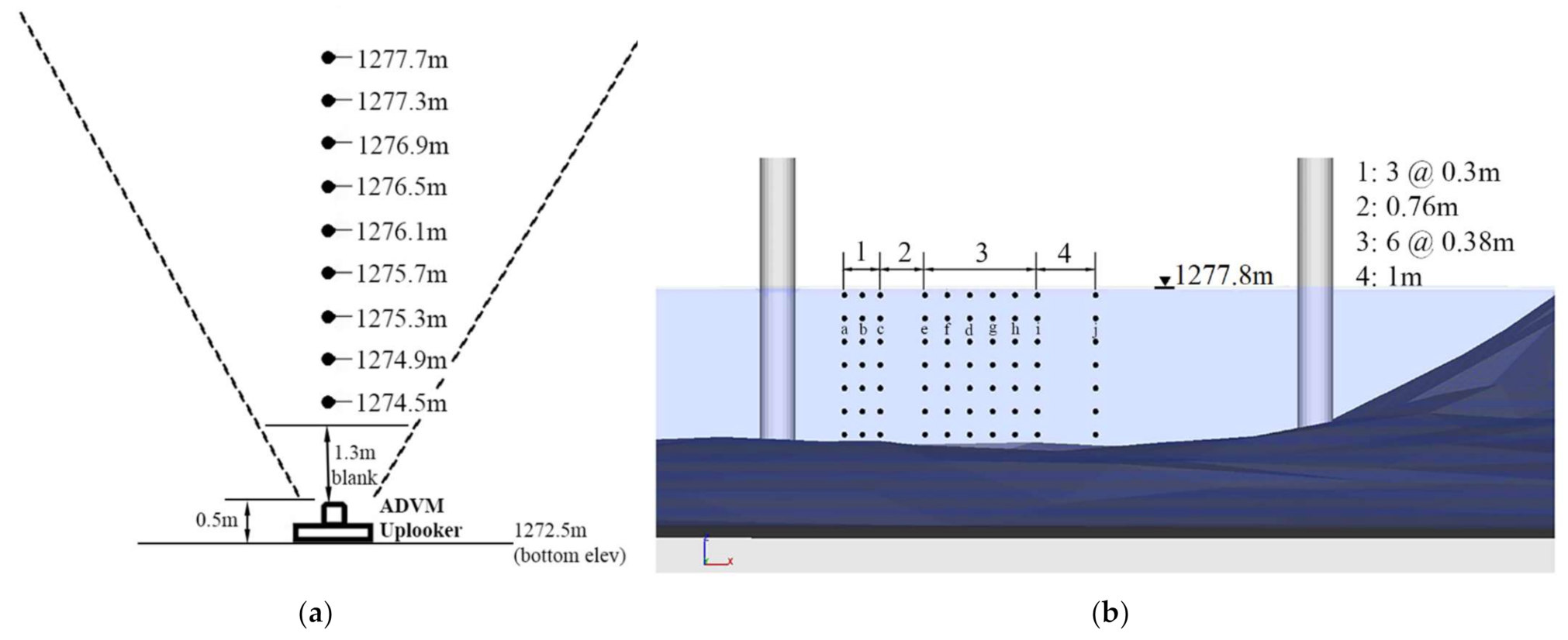
In addition to the field data collected as part of this study, the USGS and other government agencies have GSL data extending over more than 50 years. The USGS data includes various buoys measuring σ at monthly intervals located in the vicinity of the causeway (Figure 1 and Figure 4), but at a considerable distance from the breach. However, the USGS has collected samples at the WC breach at monthly intervals (locations 10010026 and 10010025) since 2017. They also have an acoustic doppler velocimeter meter (ADVM) uplooker at the WC breach that is adjacent to a row of piers, directly below the north face of the bridge decking (see Figure 4). The ADVM sensor is approximately 0.5 m above the lake bottom and begins sampling 1.3 m above the lake bottom. The USGS estimates velocity profiles at this location using the Index Velocity Method [30] with corresponding index rating and 9 vertical bins. During this study ADVM data were shared with USU, but the official review and online publication of the data by the USGS was underway and had not yet been completed. Due to uncertainty in the specific location of the ADVM relative to the pier in the transverse direction, the CFD portion of this study considered vertical profiles at 10 distances from the respective piers selected based upon information gathered from the USGS (Figure 4b). In addition to salt concentrations and velocity measurements, the USGS collects WSE data at an adjacent pier in the northern section (See Figure 3b), at a pier to the east of the WC breach in the southern section, and at the breach (Figure 2a).
The CFD model required density inputs for the boundary conditions on the north and south sections of the lake. Field instrumentation provided σ and water temperature data to estimate water densities, ρ, using linear interpolation of the USGS data [31], data provided to the USGS from monitoring during and after construction [32,33], and data collected as part of this modeling effort. In addition to σ, the TDS was also referenced for selecting density, with a conversion from TDS to density via a conversion equation employed by the USGS [17]. The final range of north and south densities selected for CFD testing was based upon the continuous σ measurements, TDS measurements taken for this study (USU UWRL), and the monthly USGS TDS measurements.
3.2. Numerical Model
3.2.1. Model Overview and Flow Equations
FLOW-3DTM by Flow Science, Inc.© was used to numerically simulate the density-driven flow through the WC breach for the typical bidirectional case (surface flows to the north with subsurface flows to the south). This solver uses the Navier–Stokes equations with a finite v-volume method with the free-surface (air–water boundary) resolved spatially and temporally via the FLOW-3D Volume-of-Fluid (TruVOF) method, [34]. The CFD model development included an initial phase where different aspects of the model were tested in a sectional slice (2D setup) with the spanwise direction represented using a single cell thick layer of elements. This was followed by the main phase in which simulations were conducted with the computational domain covering the entire breach and adjacent portions of the lake and breach (3D setup). The computational element sizes used in the 2D and 3D setup simulations were the same. The 2D simulations were primarily used to ascertain the most appropriate turbulence model to be used. FLOW-3D has multiple turbulence closures, including one that uses a large eddy simulation (LES) like approach to calculate the turbulent eddy viscosity. The Reynolds-averaged Navier–Stokes equations under the Boussinesq approximation are solved along with the conservation of mass, and a scalar/density transport equation that models the transport of salt. The equations solved are:
where VF is the fractional volume of flow, xi represents the selected cartesian coordinate, Gi and fi are the body and viscous accelerations, respectively. Ai is the fractional area open to flow in a particular direction, ui is the mean velocity, p is the pressure, is the density of the flow, is the reference density (which is the same as the density of south side of the lake), and K is summation of molecular and turbulent diffusivity of the transported salt. In Equation (1), fi is defined as:
Sij is the strain rate tensor, is the wall shear stress, is the total dynamic viscosity, which encapsulates both the molecular and turbulent eddy viscosity (). The differences between all the turbulence models tested for the study is due to the different approaches adopted to caclulate the turbulent eddy viscosity () [35].
This study tested four turbulence schemes: the k-ε, the RNG k-ε, k-ω, and LES. Equations (6)–(8) are used to determine k and ε in the standard k-ε model.
with C1 = 1.44, C2 = 1.92, Cν = 0.09, and the Prandtl number of turbulence for ε and k are σε = 1.3 and σk = 1.0, respectively. The RNG k-ε model (Equations (9) and (10)) with turbulence viscosity determined via Equation (11) and μ = νρ:
where k is the turbulent kinetic energy (TKE), ε the rate of dissipation of k, μ dynamic viscosity, μt turbulent dynamic viscosity, and Pk is the production of k, and C1ε = 1.39, C2ε = 1.42 and Cμ = 0.085. The k-ω model is Equations (12)–(14):
where σω = 0.5 and σk = 0.5, α = 0.52, β = 0.072fB and β* = 0.09f*B. Finally, the LES solver used herein is the Smagorinsky model [36,37] that computes all turbulent flow structures that can be resolved by the computational grid. Sub-grid turbulence effects are modeled through the turbulent eddy viscosity (), calculated using Equations (15)–(17):
where c is the Smagorinsky coefficient defined as 0.1 [38], l is the sub-grid length scale and S is the strain rate tensor, and is the strain rate tensor and is defined as . is the size of the element in the x-direction.
The aforementioned turbulence closure schemes were tested during the 2D modeling phases, and the best performance (relative to field data) was given by the LES and the k-ω models. Interestingly, use of the LES model (compared to k-ω) resulted in a reduction in wall-clock time by about 30% for 2D simulations. Due to these factors, the turbulence closure used for the final 3D phase of modeling was LES. The turbulence closure models did not have a term explicitly to account for stratification driven turbulence dissipation. Though requirement of that component in the models has been found to be more important for modeling turbulence in a stably-stratified setup [39]. Previous studies have shown that accounting for stratification effects in turbulence closures have less significance for modeling accelerating gravity current dynamics [35,40].
The first-order momentum advection scheme and first-order volume-of-fluid advection were used with an implicit pressure solver with the generalized minimum residual (GMRES) method (no over- or under- relaxation) with the subspace size of 15, inter-block boundary coefficient of 0.25, and volume fraction cleanup of 0.05. The bathymetry, causeway, and piers were numerically represented as solids by the Fractional Area/Volume Obstacle Representation (FAVOR) method. In order to reduce numerical diffusion and increase accuracy in solving the density transport equation, the second-order monotonicity preserving scheme was used. Other lower-order options (e.g., first-order approximation) were also tested and were found to give erroneous results.
3.2.2. Model Domain and Boundary Conditions
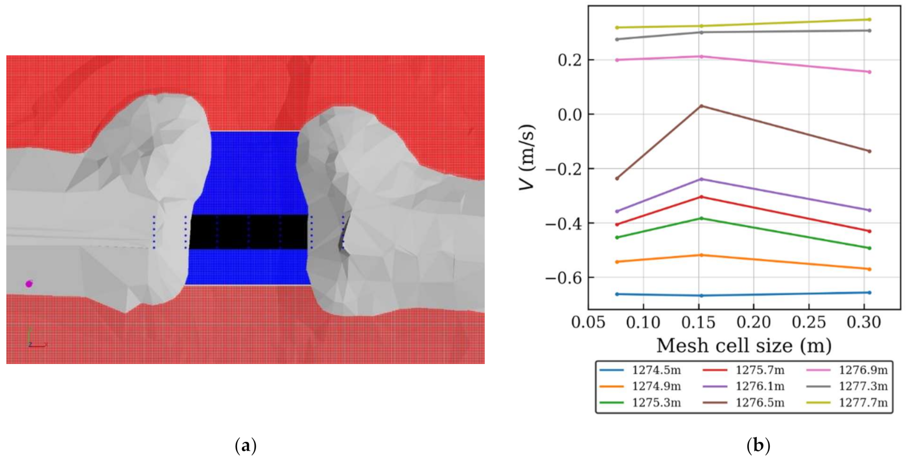
The 3D numerical domain was 295 m by 275 m centered on the breach (Figure 5). Hexahedral cells of different dimensions were employed to resolve different parts of the domain (Figure 6a). Grid convergence [41] was studied for both 2D and 3D models, where the grid convergence for the 2D model included eight cell sizes refinements ranging from 0.3 m to 0.03 m, and the grid convergence for the 3D model included three cell size refinements ranging from 0.3 m to 0.08 m. Results from the grid-convergence indicated solution independence was achieved for cells of 0.15 m (see Figure 6b). For this study the final discretization of the main phase domain was comprised of two mesh blocks of 0.3 m cubic cells linked in series, with two nested blocks with 2:1 cell refinement at the boundary (i.e., the second nested block cell size was x = y = z = 0.08 m). The number of cells in the final 3D simulations were 23.4 million.
The northern boundary conditions were assigned a WSEN of 1277.76 m and density of ρn = 1180.22 kg/m3, based upon field data (noted in red region as P in Figure 5). Similarly, the southern boundary conditions were assigned a WSES of 1277.82 m, or 0.06 m higher with density of ρs =1097.75 kg/m3 (noted as P in blue region in Figure 5). The boundaries where WSE is assigned are specified as pressure boundaries of the type that allows free inflow/outflow of water and corresponding flow properties, including variable water densities, are tracked and corresponding advective scalars are prescribed at the boundary along with a hydrostatic pressure distribution. The top boundary was defined as a Dirichlet boundary condition with atmospheric pressure set to 0 or the gage pressure. Note that diffusion at the fluid–no fluid interface is managed by a fluid-volume correction (<±0.01%). The wall boundary condition (bottom, all solids, etc.) were prescribed as a no-slip surface condition where the solver checks for laminar or turbulent flow conditions in a cell at the boundary and then prescribes an appropriate log-velocity profile and a zero tangential velocity at the wall. FLOW-3D also considers smooth vs. rough wall logarithmic expressions via a modified viscosity that reflects enhanced momentum exchange due to a roughness height:
where utan is the tangential velocity at the wall at a distance from the wall y, κ is the von Karman coefficient, us is shear velocity, a is a constant equal to 0.246 (rough wall boundary), and ks is a user-defined roughness height. Due to the macro-roughness features through the breach, ks is not significant and with a negligible roughness height, good agreement was obtained in the velocity profile discussed in Section 4. Note that local velocities are used as expected to compute wall shear stresses and are included as required as transport parameters in corresponding turbulence models. Based upon the final selected mesh size y+ values close to the boundary are about 5000, which is much higher than those used by boundary-resolved LES simulations where y+ < 10.
Initial boundary conditions were defined for each main mesh block with fixed water surface elevations and water densities corresponding to the respective northern and southern boundaries. All the simulations were monitored and run long enough to reach a steady state for the given boundary conditions.
4. Results and Discussion
4.1. Density and Water Surface Elevations
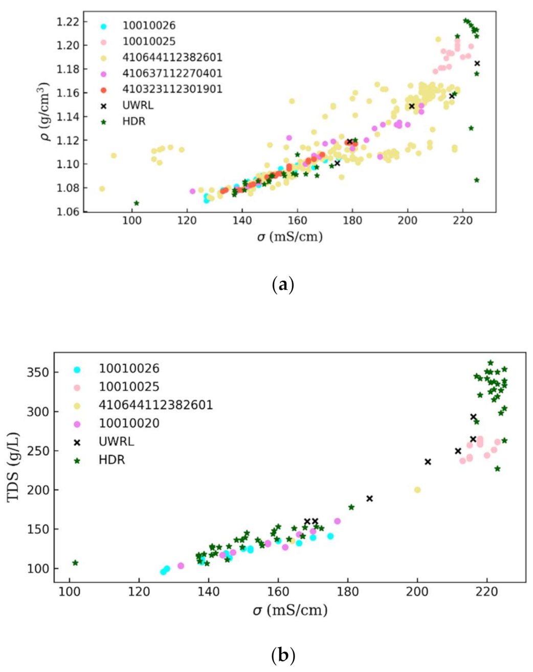
As previously noted, USGS has multiple buoys in the GSL where grab samples are analyzed for TDS along with corresponding σ. USGS calculates ρ as a function of TDS via Equation (19) from [17]:
where TDS is in g/mL and ρ is in g/L at 20 °C. Therefore, to directly compare ρ collected from this study (identified in Figure 7 as UWRL data) to USGS data the same technique was adopted. Naftz et al. [42] developed an equation of state for the hypersaline water from the southern part of GSL, where ρ can be computed as a function of temperature and salnity. The Naftz et al.’s equation of state was not useful for the current study due to lack of a relationship between specific conductance and salinity, and also the fact that the aforementioned equation was developed only using data from the south part of GSL. Note that since 2016, a private consultancy HDR was also monitoring ρ at the new breach on behalf of the Union Pacific Railroad and they also adopted the USGS approach; these three data sets are presented in Figure 7.
These data in addition to the σ measurements made by the authors served as the basis of choosing ρS and ρN used in the model simulations. Note that the CFD simulations require that ρ be in units of kg/m3, thus the density difference Δρ is provided accordingly.
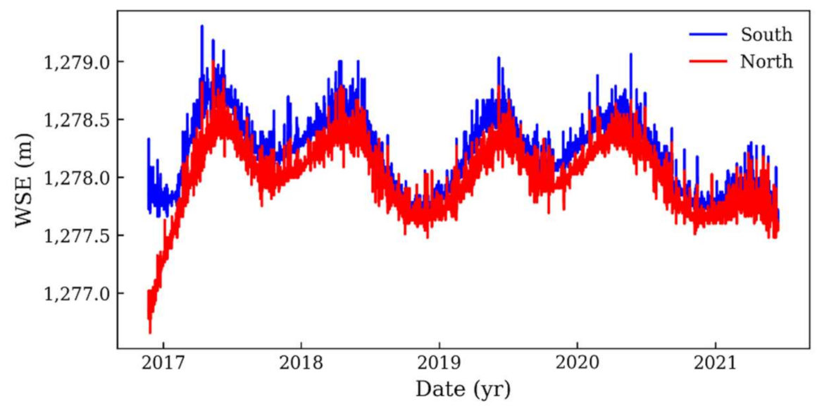
In addition to Δρ, the bidirectional flow patterns in the WC Breach are also influenced by water surface elevations; the continuous measurements of USGS for north and south water surface elevations near the breach for the entire period since the WC Breach was completed are also shown (Figure 8). From this data, a specific day corresponding to ADVM measurements and TDS measurements was selected for modeling (Table 1).
Some variability in field measurements is likely due to instrument accuracy (Figure 7 and Figure 8) and also due to lake dynamics and temporal variations in response to climate, weather patterns, etc. These factors were considered when selecting boundary conditions for the CFD simulations. A case that is representative of the density driven bidirectional flow patterns was selected. Specific velocity data and corresponding WSEs were used in the modeling and a sensitivity analysis of densities and velocity profile location was completed.
4.2. Model Comparison with Field Measurements
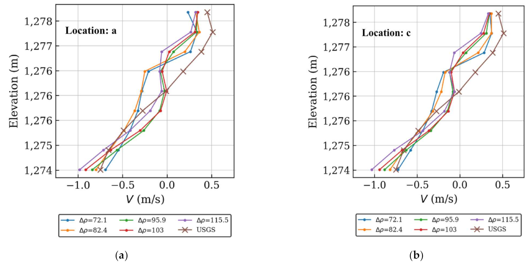
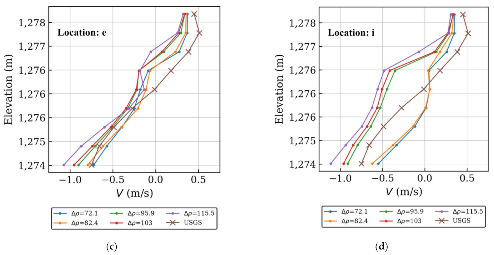
Once the mesh resolution study was completed, the accuracy of the 3D model was tested against the unpublished USGS velocity profile measured at the WC breach (Figure 6). Several unknown parameters needed to be considered while comparing the CFD model results with the field measurements. First, the exact density difference Δρ between the northern and southern sections of the lake is uncertain. As described in Section 3.1 and Figure 4, the field data, including the time-series of σ, indicated that there was a small range of possible ρ values for the northern part of the lake. Thus, for the 5 cases considered below, different densities between the northern and southern sections of the lake were simulated (Table 1).
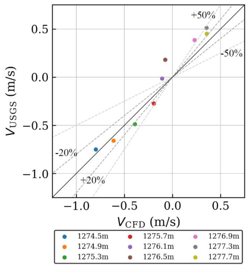
The second source of uncertainty was the exact location of the ADVM uplooker with respect to the central column of piers at the WC breach. It is known that the uplooker is located slightly north of the northern-most pier in the center column, and within 1.5–2.5 m east of the that pier. However, to ascertain the potential location of the uplooker, the streamwise velocity was probed at multiple locations east of the pier (Figure 4) and the locations were investigated using different density differences (Figure 9). The results show that the correct density difference, Δρ, between the northern and southern sides is ~82.4 kg/m3, and the location of the uplooker is about 1.5 m east of the pier. Given the uncertainty in the field data and its location, the comparison between the measured and computed velocity (V) profiles is satisfactory (Figure 10). The only points in the profile that do not compare well, which have more than 50 percent error, are V at the interface of the north–south and south–north flows. This is not unexpected, as there is some uncertainty in the field velocity profile at this interface and this section is more challenging to simulate numerically as there is a sudden change in density and velocity.
4.3. Simulated Flow Field
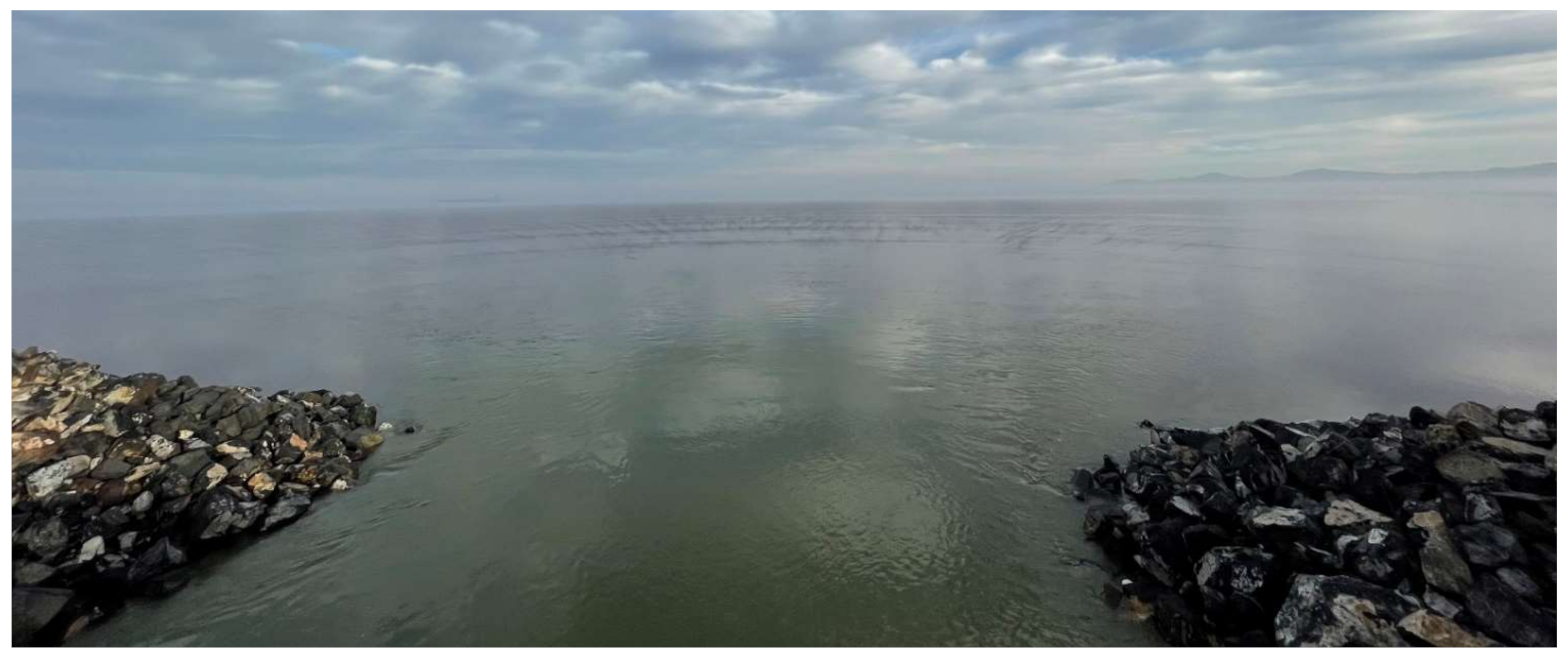
Based on the field observations (Figure 11) and field data, the general dynamics of the flow is clear; hypersaline water from the north side of the lake plunges below the south side water that is flowing south to north (S-N) just before entering the breach. This creates a relatively thick and denser bottom current flowing north to south (N-S), and a relatively thinner and less dense S-N current flowing at the surface. As this top current exits the breach it spreads longitudinally and laterally, and thins as it travels north, with its thickness decreasing with distance away from the breach. To provide a general overview of the hydrodynamics at the breach, ρ and the S-N (y-direction) velocity V has been plotted for the vertical-plane orthogonal to the x-axis and going through the center of the breach (Figure 12 and Figure 13). CFD results clearly capture the dynamics observed in the field and the simulation results provide more insights about the formation of the density driven bidirectional flow pattern (N-S and S-N currents). In agreement with field observations, the thickness of the distinct layers of the flow are similar with the bottom layer being relatively thick with a non-negligible velocity. The hypersaline water from the north maintains its thickness some distance from the causeway, eventually forming the DBL. The hypersaline northern current also appears to go through a subsurface hydraulic jump just after it plunges and before entering the central part of the breach, which is a function of the submerged dike or berm specifically placed to manage flows through the WC breach. The hypersaline N-S current can be seen to accelerate just after plunging under the incoming S-N flow. The S-N flow also accelerates while going through the breach and can be seen to travel much further into the northern side than the density plots indicate. In order to get a clearer view of the flow evolution, vertical planes orthogonal to the S-N (y-direction) direction have been plotted at 12-m intervals starting south of the breach (Figure 14).
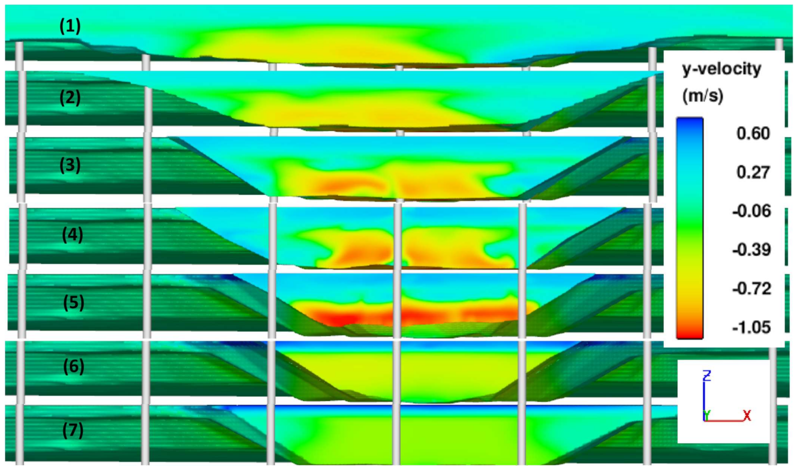
It can be observed that the flow has a clear bidirectional form, though the thickness of the N-S bottom current and the S-N top layer flow change spatially (Figure 14). It was observed that a distinct N-S flowing bottom layer, which is still relatively thick, is primarily confined to the center of the channel at location 1 (Figure 14 top). The flow has expanded laterally, but is still mostly flowing along the channel that was dredged during breach construction. Charting the evolution of the N-S current, starting from the northernmost slice at location 7 (Figure 14 bottom), it is observed that the current accelerates and decreases in thickness as it approaches the breach. The current accelerates from about 0.2 m/s to about 1 m/s in a span of about 24 m. The approximate densimetric Froude number of the bottom current at the location of the uplooker measurement is about 0.7. Thus, there is a chance that the flow might become supercritical while accelerating towards the breach, justifying that hydraulic jump is plausible. Additionally, the piers of the breach can be observed to have induced mixing and decrease the density stratification. This can be inferred from the sudden increase in bottom layer thickness going from location 5 to location 4 (Figure 14). The effect of the piers on the structure of the N-S current can be observed 12 m downstream (see Figure 14, location 3). Going further south, the bottom current further decreases in thickness (see Figure 12), but retains velocities around 0.8–0.9 m/s. This N-S current transforms to become the dense DBL.
The S-N flow, which is confined to the top layer of the water column, can be observed to be accelerating while approaching the breach. While flowing among the piers, the S-N flow covers more area in the cross-section than the N-S flow. Though by the time the flow passes through the breach (Figure 14, location 5), the water column has been divided into two distinct parts. Within 24 m, the S-N current gets confined within 1/10th of the water column, while accelerating to about 0.6 m/s. This S-N current now has a densimetric Froude number of about 1.2 and is supercritical.
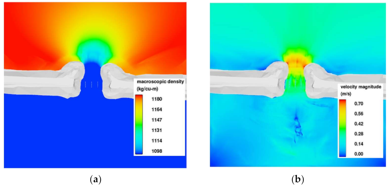
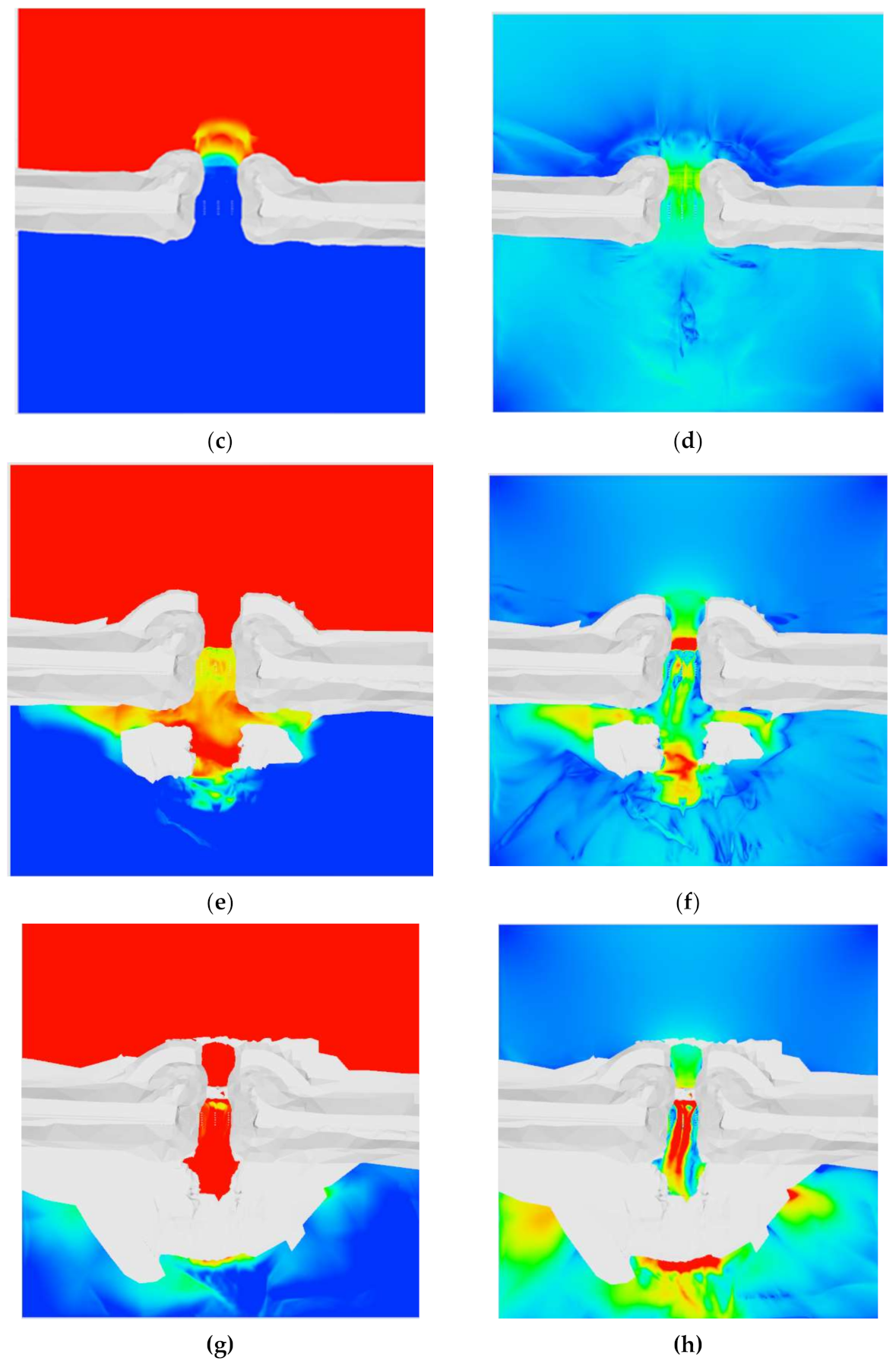
In order to further understand what the flow looks like at different elevations, density and velocity magnitudes at four different layers have been plotted in Figure 15. The flow at the surface is primarily S-N, and the current can be seen to be expanding radially away from the WC breach. This matches with the field observations, where this current confined to the top-layer of the water column was observed beyond 1000 m north of the WC breach. The next layer at 1.1 m from the surface, the flow has relatively high velocity while going through the breach, especially once the S-N flow has crossed the piers and is pushed further up in the water-column. The next layer at 2.5 m below the surface, the flow is dominated by the N-S current, though there are parts where this layer is near/passing-through the interface between the two currents. The bottom current can be observed passing through the breach and continuing along the central-channel (Figure 15g), while a portion travels laterally. This plunging of the N-S current might lead to overturning of the flow, leading to enhanced mixing near the edges of the breach on the south side (Figure 14 location 3). The N-S current also seem to go through relatively high acceleration after entering the breach (Figure 14, location 6), and this is also the zone where the N-S current plunges towards the bottom. The layer at about 3.4 m from the surface (Figure 15g,h) is dominated by the bottom hugging N-S current. High velocities are observed within the dredged channel.
These modeling results also highlight the role of bottom topography in the bottom current behavior. The distinct berm (bottom sill) is observed North of the breach, which can be used to reduce the N-S flow, and consequently the DBL. Though how effective it will be, or how high it has to be made to impact the DBL is not well understood. It can also be observed that the bottom of the lake on the southern side increases in elevation just after the dredged region of the breach. This will have a significant effect on the mechanism of the DBL formation, and will be studied in detail in the future. This CFD model can also be modified and used to study the effect of the berm.
For the purpose of developing an accurate water and salt balance model of the lake, it is important to accurately estimate the north and south flows through the breach. The results of this study indicate that the CFD model can be used to simulate other lake levels and water density variability that could be combined to develop a more robust rating curve for the breach. Furthermore, this model can be a used as a forecasting tool to anticipate future conditions as lake levels continue decreasing to unprecedented conditions resulting from extended periods of drought.
5. Conclusions
The density-driven bidirectional current through the recently completed West Crack breach at the Great Salt Lake causeway was simulated with an LES CFD model to support management efforts that include environmental and economic concerns. Modeling was based upon field campaigns and datasets provided by the USGS. Results from this study indicate that the vertical velocity profile in the breach had good agreement with unpublished USGS velocity profile data with an R2 = 0.9578 and generally within 20 to 50% at different depths throughout the water column in the breach. The model is sensitive to density differences between flow layers along with breach geometry and water surface elevations, which is also the case for lake flows through the WC breach. The model resulting from this work can be used to better approximate water and salt exchanges between the north and south sides of the GSL, provide insight into future management of the lake, and be applied as a forecasting tool to anticipate future lake conditions.
Author Contributions
Conceptualization, S.D. and B.M.C.; methodology, S.D. and B.M.C.; software, M.R., B.M.C. and S.D.; validation, M.R., B.M.C. and S.D.; formal analysis, M.R., B.M.C. and S.D.; investigation, B.T.N., B.M.C., M.R. and S.D.; resources, S.D. and B.M.C.; data curation, M.R.; writing—original draft preparation, B.M.C. and S.D.; writing—review and editing, B.T.N., S.D., M.R. and B.M.C.; visualization, M.R.; supervision, S.D. and B.M.C.; project administration, S.D.; funding acquisition, S.D. and B.M.C. All authors have read and agreed to the published version of the manuscript.
Funding
This research was funded by the Utah Department of Natural Resources through the 2020 Division of Forestry, Fire, and State Lands Grant. This research was also funded by the State of Utah though Utah State University and the Utah Water Research Laboratory.
Institutional Review Board Statement
Not applicable.
Informed Consent Statement
Not applicable.
Data Availability Statement
Some or all data, models or code that support the findings of this study are available from the corresponding authors upon reasonable request. Please not that at the time of this study the USGS velocity data was preliminary as it had not yet completed final review and publication of data online per the USGS policy.
Acknowledgments
The authors thank David Tarboton for their support of this study. The authors would like to thank Utah DNR for sponsoring this research, and the USGS Great Salt Lake office, specifically Ryan Rowland, Michael Freeman, and Travis Gibson, for all the help they have provided during the field campaign and the clarifications about the data they have been collecting.
Conflicts of Interest
The authors declare no conflict of interest. The funders had no role in the design of the study; in the collection, analyses, or interpretation of data; in the writing of the manuscript, or in the decision to publish the results.
References
- Messager, M.L.; Lehner, B.; Grill, G.; Nedeva, I.; Schmitt, O. Estimating the volume and age of water stored in global lakes using a geo-statistical approach. Nat. Commun. 2016, 7, 13603. [Google Scholar] [CrossRef]
- Pendleton, M.C.; Sedgwick, S.; Kettenring, K.M.; Atwood, T.B. Ecosystem functioning of Great Salt Lake wetlands. Wetlands 2020, 40, 2163–2177. [Google Scholar] [CrossRef]
- Conover, M.R.; Bell, M.E. Importance of Great Salt Lake to pelagic birds: Eared grebes, phalaropes, gulls, ducks, and white pelicans. In Great Salt Lake Biology; Springer: Cham, Switzerland, 2020; pp. 239–262. [Google Scholar]
- Wurtsbaugh, W.A.; Miller, C.; Null, S.E.; DeRose, R.J.; Wilcock, P.; Hahnenberger, M.; Moore, J. Decline of the world’s saline lakes. Nat. Geosci. 2017, 10, 816–821. [Google Scholar] [CrossRef]
- Mischke, S.; Liu, C.; Zhang, J.; Zhang, C.; Zhang, H.; Jiao, P.; Plessen, B. The world’s earliest Aral-Sea type disaster: The decline of the Loulan Kingdom in the Tarim Basin. Sci. Rep. 2017, 7, 43102. [Google Scholar] [CrossRef] [PubMed]
- AghaKouchak, A.; Norouzi, H.; Madani, K.; Mirchi, A.; Azarderakhsh, M.; Nazemi, A.; Hasanzadeh, E. Aral Sea syndrome desiccates Lake Urmia: Call for action. J. Great Lakes Res. 2015, 41, 307–311. [Google Scholar] [CrossRef]
- Gross, M. The world’s vanishing lakes. Curr. Biol. 2017, 27, 43–46. [Google Scholar] [CrossRef]
- Jellison, R.; Williams, W.D.; Timms, B.; Alocer, J.; Aladin, N.V. Aquatic Ecosystems: Trends and Global Prospects; Polunin, N.V.C., Ed.; Cambridge University Press: Cambridge, UK, 2008; pp. 94–112. [Google Scholar]
- Case, H.L.I. Salton Sea Ecosystem Monitoring and Assessment Plan Open-File Report 2013–1133; United States Geological Survey: Reston, VA, USA, 2013.
- Barnes, B.D.; Wurtsbaugh, W.A. The effects of salinity on plankton and benthic communities in the Great Salt Lake, Utah, USA: A microcosm experiment. Can. J. Fish. Aquat. Sci. 2015, 72, 807–817. [Google Scholar] [CrossRef]
- Naftz, D.L.; Cederberg, J.R.; Krabbenhoft, D.P.; Beisner, K.R.; Whitehead, J.; Gardberg, J. Diurnal trends in methylmercury concentration in a wetland adjacent to Great Salt Lake, Utah, USA. Chem. Geol. 2011, 283, 78–86. [Google Scholar] [CrossRef]
- White, J.S.; Null, S.E.; Tarboton, D.G. How do changes to the railroad causeway in Utah’s Great Salt Lake affect water and salt flow? PLoS ONE 2015, 10, e0144111. [Google Scholar] [CrossRef] [PubMed] [Green Version]
- Null, S.E.; Wurtsbaugh, W.A.; Miller, C. Can the causeway in the Great Salt Lake be used to manage salinity? Friends Great Salt Lake Newsl. 2013, 19, 14. [Google Scholar]
- Bioeconomics, Inc. Economic Significance of the Great Salt Lake to the State of Utah. Prepared for State of Utah Great Salt Lake Advisory Council. 2012. Available online: http://www.gslcouncil.utah.gov/docs/GSL_FINAL_REPORT-1-26-12.PDF (accessed on 1 June 2021).
- Wurtsbaugh, W.; Miller, C.; Null, S.; Wilcock, P.; Hahnenberger, M.; Howe, F. Impacts of Water Development on Great Salt Lake and the Wasatch Front. In White Paper to the Utah State Legislature. Prepared by Utah State University; Utah State University: Salt Lake City, UT, USA, 2016. [Google Scholar]
- WHSRN. Western Hemisphere Shorebird Reserve Network. 2016. Available online: www.whsrn.org (accessed on 1 May 2021).
- Loving, B.L.; Waddell, K.M.; Miller, C.W. Water and Salt Balance of Great Salt Lake, Utah, and Simulation of Water and Salt Movement through the Causeway, 1987–1998; U.S.G.S Water-Resources Investigations Report 00-4221; U.S. Geologic Survey: Salt Lake City, UT, USA, 2000.
- Waddell, K.M.; Bolke, E.L. The Effects of Restricted Circulation on the Salt Balance of Great Salt Lake, Utah; Bulletin 18; Utah Geological Survey Water Resources: Salt Lake City, UT, USA.
- Stephens, D.W. Changes in lake levels, salinity and the biological community of Great Salt Lake (Utah, USA), 1847–1987. Hydrobiologia 1990, 197, 139–146. [Google Scholar] [CrossRef]
- Rupke, A.L.; McDonald, A. Great Salt Lake Brine Chemistry Database, 1966–2011; Open-File Report 596, compact disk; Utah Geological Survey: Reston, VA, USA, 2012.
- Baxter, B.K. Great Salt Lake microbiology: A historical perspective. Int. Microbiol. 2018, 21, 79–95. [Google Scholar] [CrossRef] [Green Version]
- Yang, S.; Johnson, W.P.; Black, F.J.; Rowland, R.; Rumsey, C.; Piskadlo, A. Response of density stratification, aquatic chemistry, and methylmercury to engineered and hydrologic forcings in an endorheic lake (Great Salt Lake, USA). Limnol. Oceanogr. 2020, 65, 915–926. [Google Scholar] [CrossRef]
- Holley, E.R.; Waddell, K.M. Stratified Flow in Great Salt Lake Culvert. J. Hydraul. Div. 1976, 102, 969–985. [Google Scholar] [CrossRef]
- Spall, R.E. A Hydrodynamic Model of the Circulation within the South Arm of the Great Salt Lake. Int. J. Model. Simul. 2009, 29, 181–190. [Google Scholar]
- Spall, R.E. Basin-Scale Internal Waves within the South Arm of the Great Salt Lake. Int. J. Model. Simul. 2011, 31, 25–31. [Google Scholar] [CrossRef]
- Dutta, S.; Tokyay, T.E.; Cataño-Lopera, Y.A.; Serafino, S.; Garcia, M.H. Application of computational fluid dynamic modelling to improve flow and grit transport in Terrence J. O’Brien Water Reclamation Plant, Chicago, Illinois. J. Hydraul. Res. 2014, 52, 759–774. [Google Scholar] [CrossRef]
- Crookston, B.M.; Anderson, R.M.; Tullis, B.P. Free-flow discharge estimation method for Piano Key weir geometries. J. Hydro-Environ. Res. 2018, 19, 160–167. [Google Scholar] [CrossRef]
- Standard Methods. 2540 C, 2540 D, 2540 E, APHA, AWWA, and WEF 2014. Standard Methods for the Analysis of Water and Wastewater Online. Available online: www.standardmethods.org (accessed on 1 July 2021).
- In-Situ. Aqua TROLL ® 600 Multiparameter Sonde 2020. Available online: https://in-situ.com/pub/media/support/documents/AquaTROLL600_Spec-Sheet.pdf (accessed on 1 August 2021).
- Levesque, V.A.; Oberg, K.A. Computing Discharge Using the Index Velocity Method; U.S. Geological Survey: Reston, VA, USA, 2012; 148p.
- U.S. Geological Survey (USGS). National Water Information System Data for the Nation. 2020. Available online: https://waterdata.usgs.gov/nwis/ (accessed on 15 June 2021).
- HDR 2019 Annual Data Monitoring Report 2020. Available online: https://documents.deq.utah.gov/water-quality/standards-technical-services/gsl-website-docs/uprr-causeway/DWQ-2020-003963.pdf (accessed on 15 November 2020).
- HDR 2020 Annual Data Monitoring Report 2021. Available online: https://documents.deq.utah.gov/water-quality/standards-technical-services/gsl-website-docs/uprr-causeway/DWQ-2021-002902.pdf (accessed on 15 November 2020).
- Hirt, C.W.; Nichols, B.D. Volume of fluid (VOF) method for the dynamics of free boundaries. J. Comput. Phys. 1981, 39, 201–225. [Google Scholar] [CrossRef]
- Stancanelli, L.M.; Musumeci, R.E.; Foti, E. Computational fluid dynamics for modeling gravity currents in the presence of oscillatory ambient flow. Water 2018, 10, 635. [Google Scholar] [CrossRef] [Green Version]
- Smagorinsky, J. General circulation experiments with the primitive equations: I. The basic experiment. Mon. Weather Rev. 1963, 91, 99–164. [Google Scholar] [CrossRef]
- Germano, M.; Piomelli, U.; Moin, P.; Cabot, W.H. A dynamic subgrid-scale eddy viscosity model. Phys. Fluids A Fluid Dyn. 1991, 3, 1760–1765. [Google Scholar] [CrossRef] [Green Version]
- Pope, S.B. Turbulent Flows; Cambridge: Cambridge, UK, 2001. [Google Scholar]
- Yeh, T.H.; Cantero, M.; Cantelli, A.; Pirmez, C.; Parker, G. Turbidity current with a roof: Success and failure of RANS modeling for turbidity currents under strongly stratified conditions. J. Geophys. Res. Earth Surf. 2013, 118, 1975–1998. [Google Scholar] [CrossRef] [Green Version]
- An, S.; Julien, P.Y.; Venayagamoorthy, S.K. Numerical simulation of particle-driven gravity currents. Environ. Fluid Mech. 2012, 12, 495–513. [Google Scholar] [CrossRef]
- Roache, P.J. Verification and Validation in Computational Science and Engineering; Hermosa: Albuquerque, NM, USA, 1998; p. 895. [Google Scholar]
- Naftz, D.L.; Millero, F.J.; Jones, B.F.; Green, W.R. An equation of state for hypersaline water in Great Salt Lake, Utah, USA. Aquat. Geochem. 2011, 17, 809–820. [Google Scholar] [CrossRef]
Figure 1.
The Great Salt Lake located in the state of Utah, USA. Insets show the causeway that divides the lake into a Northern section and Southern section, and the location of the West Crack (WC) Breach in the causeway. The USGS measurement stations used to set the boundary conditions within the CFD model are also shown.

Figure 2.
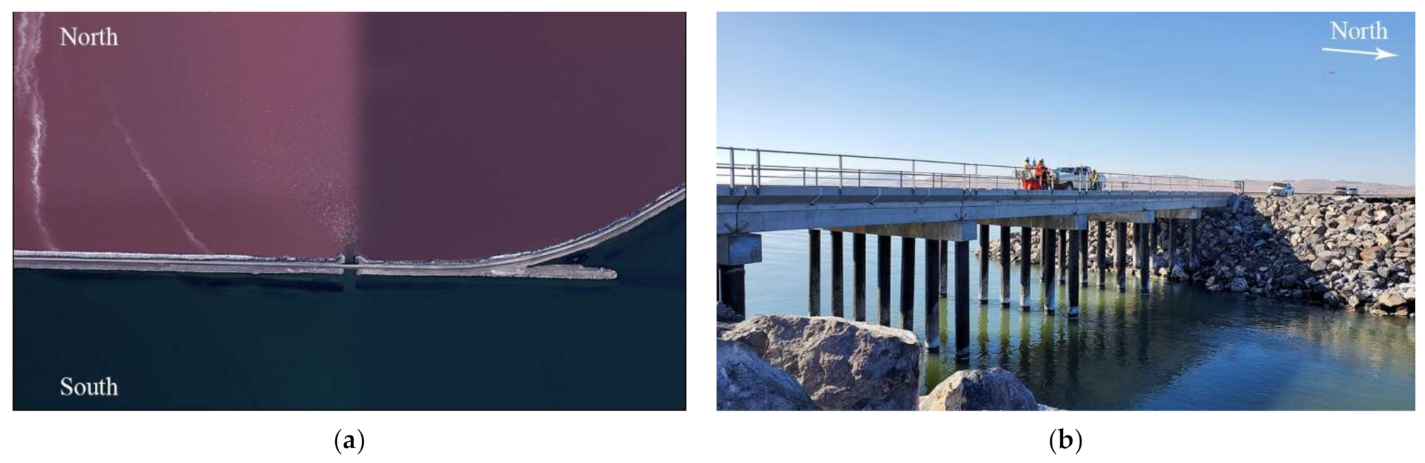
(a) Satellite image of the causeway and the West Crack (WC) Breach. The hyper-saline northern part of the lake has a pink color due to presence of microbes that thrive in the hyper-saline environment [21] (b) Picture of the WC Breach taken from the northern side of the causeway, during the field-campaign in October 2020. The picture illustrates the breach structure, showing the three rows of six submersed piers that affect flow through the breach.
Figure 2.
(a) Satellite image of the causeway and the West Crack (WC) Breach. The hyper-saline northern part of the lake has a pink color due to presence of microbes that thrive in the hyper-saline environment [21] (b) Picture of the WC Breach taken from the northern side of the causeway, during the field-campaign in October 2020. The picture illustrates the breach structure, showing the three rows of six submersed piers that affect flow through the breach.

Figure 3.
Field sampling for σ and TDS from shore in the southern section (a) and at a pier in the northern section (b) of the Great Salt Lake.
Figure 3.
Field sampling for σ and TDS from shore in the southern section (a) and at a pier in the northern section (b) of the Great Salt Lake.

Figure 4.
Velocity field measurement setup of the ADVM uplooker, which also corresponds to the elevations at which the CFD model is queried (a) (based on information provided by the USGS through personal communication) and sampling locations in the CFD model (b) due to uncertainty in ADVM location relative to bridge piers.

Figure 5.
The computational domain with boundary conditions of the CFD model. In the coordinate system of the model, positive X corresponds to the west-to-east direction, and positive Y corresponds to the south-to-north direction. The locations (bold-black lines) of seven vertical slices (12 m apart) in the model are also noted, which were used for analyzing the flow through the breach.

Figure 6.
An overview of the final mesh configuration with nested blocks (a). The red region has mesh size of 0.3 m, the blue region within the breach has mesh size of 0.15 m, and black region of the domain is the region surrounding the bridge piers and has a mesh size of 0.08 m. (b) The grid convergence for the 3D simulations shows that a 0.15 m mesh should be enough to capture the flow field. The velocity at nine different elevations in the water-column was monitored. Apart from one point, the streamwise (y-direction) velocity did not show appreciable change with reduction of mesh size from 0.15 m to 0.08 m. The vertical elevations where the velocity is monitored corresponded to the elevations where the USGS ADVM measured streamwise velocity (see Figure 4).

Figure 7.
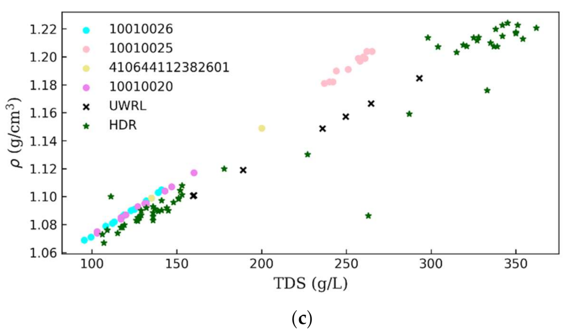
Great Salt Lake saltwater properties where monitoring locations are shown in Figure 1 with (a) density (ρ) as a function of specific conductance (σ) (b) TDS as a function of σ and (c) ρ as a function of TDS. Note that for USGS data not all parameters were collected concurrently at each gaging location.
Figure 7.
Great Salt Lake saltwater properties where monitoring locations are shown in Figure 1 with (a) density (ρ) as a function of specific conductance (σ) (b) TDS as a function of σ and (c) ρ as a function of TDS. Note that for USGS data not all parameters were collected concurrently at each gaging location.


Figure 8.
Northern and southern water surface elevations WSE for the Great Salt Lake at the West Crack Breach (completed in December 2016).
Figure 8.
Northern and southern water surface elevations WSE for the Great Salt Lake at the West Crack Breach (completed in December 2016).

Figure 9.
CFD predicted velocity profiles at the WC breach for different density differences at profile location a (a), at location c (b), at location e (c), and at location i (d). Note that locations c and e show good agreement with the USGS field data using a density difference of ~82.4 kg/m3 or simulation #2).


Figure 10.
Comparison between the measured (VUSGS) and computed (VCFD) velocity profiles at different WSE values (colored dots). For all but one point in the profile, VCFD is within 20–50 percent of the measured field data. The R2 = 0.9578.
Figure 10.
Comparison between the measured (VUSGS) and computed (VCFD) velocity profiles at different WSE values (colored dots). For all but one point in the profile, VCFD is within 20–50 percent of the measured field data. The R2 = 0.9578.

Figure 11.
View from the WC breach at the Great Salt Lake Causeway looking north. Surface flows move from south to north (bottom to top of photo). Note the radial pattern at the surface, providing indication of the relatively lighter water from the south floating over the heavier northern water. Similar radial mixing patterns at the surface can also be observed in the CFD simulation (see Figure 12).

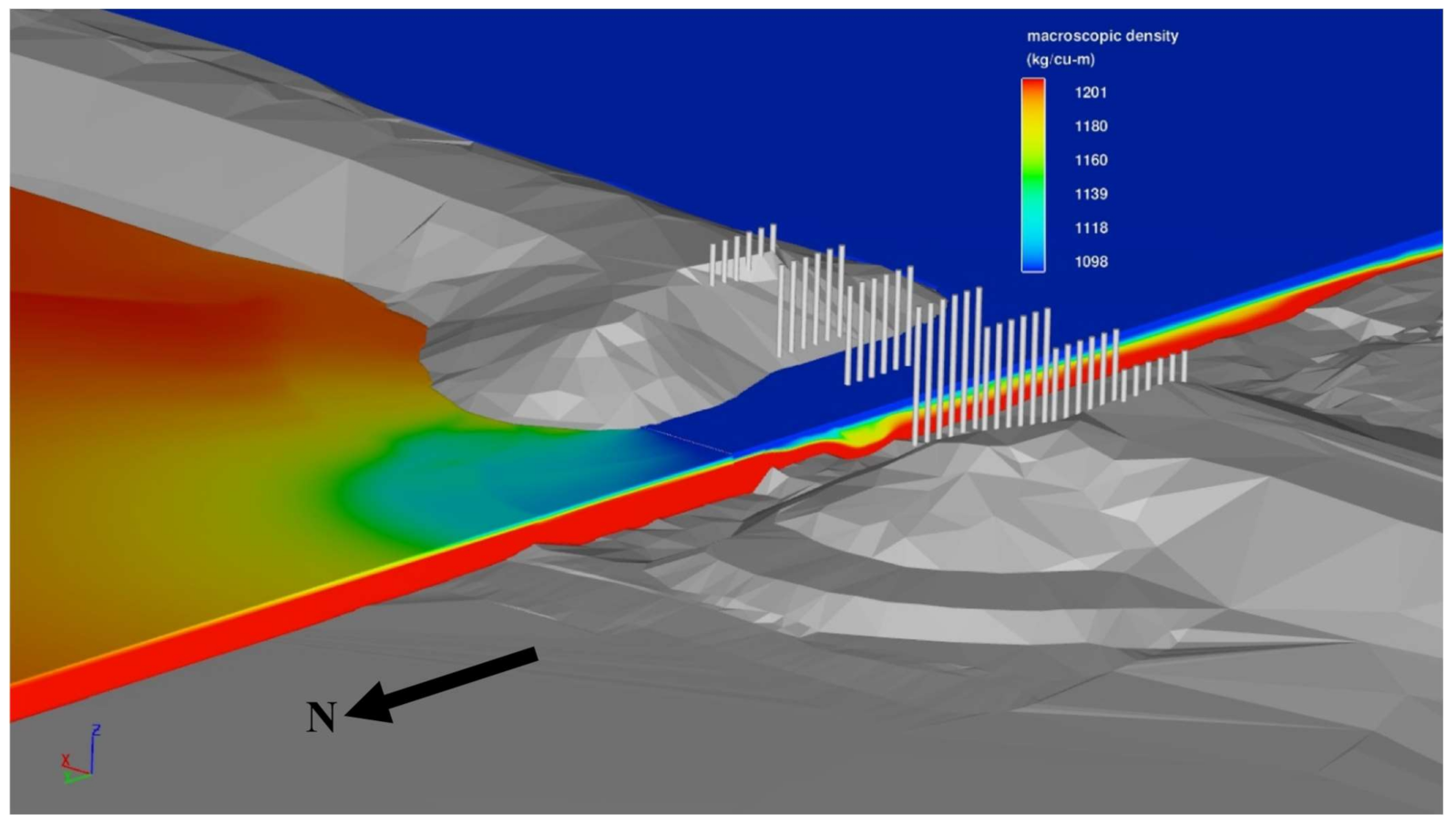
Figure 12.
Isometric view of the density within the lake. Higher density water from the north (red) plunges below the lighter water (blue) from the south. At the breach the thickness of both the layers are similar. The layer of water from the south gets appreciably thinner once it enters the northern section. The hypersaline water from the north can be seen to maintain its thickness longer, eventually forming the deep brine layer (DBL) in the south section. The hypersaline northern current also seems to go through a subsurface hydraulic jump, just after it plunges and before entering the central part of the breach.

Figure 13.
Isometric view of the velocity V in the y-direction, with the positive velocity corresponding to the south to north flow. The hypersaline N-S current can be seen to accelerate just after plunging under the incoming S-N flow. The S-N flow also accelerates while going through breach (blue) and can be seen to travel much further into the northern side than the density plots indicate.

Figure 14.
Velocity V in the y-direction at seven different vertical slices along the breach. The location of the slices has been illustrated in Figure 6. (1) Is the southernmost slice, and every slice after that is at a distance 12 m northward. The N-S current is coming out of the plane, and the S-N current is into the plane. Slices (1–3) are to the south of the piers, slices (5–7) are to the north of the piers, and slice (4) is within the columns of piers. The effect of the piers on structure of the flow, especially the N-S bottom current can be seen between (5) and (4). Effect of the piers can still be observed in (3), even though the slice is south to the piers. By the time the N-S current comes to slice (2), the effect of the piers is not evident. From (2) to (1), the hypersaline current does not show much change.

Figure 15.
CFD density driven bidirectional flow results for density (left column) and velocity magnitude V (right column) in plan view at the water surface (a,b), at 1.1 m from the surface (c,d), at 2.5 m from the surface (e,f), and near the bottom of the lakebed (3.4 m from surface) (g,h). Note that the bottom elevation of the breach is 1272.5 m and grayed out locations are high spots in the lakebed.


Table 1.
Density difference Δρ and the difference in WSE imposed for the 3D simulations. A range of Δρ was tested due to field data and corresponding uncertainty in estimation of ρN.
Table 1.
Density difference Δρ and the difference in WSE imposed for the 3D simulations. A range of Δρ was tested due to field data and corresponding uncertainty in estimation of ρN.
| Sim (#) | ρS (g/cm3) | ρN (g/cm3) | Δρ (kg/m3) | ΔWSE (m) |
|---|---|---|---|---|
| 1 | 1.0978 | 1.1699 | 72.1 | 0.061 |
| 2 | 1.0978 | 1.1802 | 82.4 | 0.061 |
| 3 | 1.0998 | 1.1957 | 95.9 | 0.061 |
| 4 | 1.0978 | 1.2008 | 103.0 | 0.061 |
| 5 | 1.09782 | 1.2127 | 115.5 | 0.061 |
Publisher’s Note: MDPI stays neutral with regard to jurisdictional claims in published maps and institutional affiliations. |
© 2021 by the authors. Licensee MDPI, Basel, Switzerland. This article is an open access article distributed under the terms and conditions of the Creative Commons Attribution (CC BY) license (https://creativecommons.org/licenses/by/4.0/).
Share and Cite
MDPI and ACS Style
Rasmussen, M.; Dutta, S.; Neilson, B.T.; Crookston, B.M. CFD Model of the Density-Driven Bidirectional Flows through the West Crack Breach in the Great Salt Lake Causeway. Water 2021, 13, 2423. https://doi.org/10.3390/w13172423
AMA Style
Rasmussen M, Dutta S, Neilson BT, Crookston BM. CFD Model of the Density-Driven Bidirectional Flows through the West Crack Breach in the Great Salt Lake Causeway. Water. 2021; 13(17):2423. https://doi.org/10.3390/w13172423
Chicago/Turabian StyleRasmussen, Michael, Som Dutta, Bethany T. Neilson, and Brian Mark Crookston. 2021. "CFD Model of the Density-Driven Bidirectional Flows through the West Crack Breach in the Great Salt Lake Causeway" Water 13, no. 17: 2423. https://doi.org/10.3390/w13172423
Note that from the first issue of 2016, this journal uses article numbers instead of page numbers. See further details here.