
Towards a High Order Convergent ALE-SPH Scheme with Efficient WENO Spatial Reconstruction
by
 , , , and
Rubén Antona
1 ,
,
Renato Vacondio
2,
Diego Avesani
1,†,
Maurizio Righetti
1 and
Massimiliano Renzi
1,*
1
Faculty of Science and Technology, Free University of Bozen-Bolzano, Piazza Università 5, 39100 Bozen-Bolzano, Italy
2
Department of Engineering and Architecture, University of Parma, Parco Area delle Scienze 181/A, 43121 Parma, Italy
*
Author to whom correspondence should be addressed.
†
Current address: Department of Civil, Environmental and Mechanical Engineering, University of Trento, via Mesiano, 77 38123 Trento, Italy.
Water 2021, 13(17), 2432; https://doi.org/10.3390/w13172432
Submission received: 24 July 2021
/
Revised: 29 August 2021
/
Accepted: 30 August 2021
/
Published: 4 September 2021
(This article belongs to the Section Hydraulics and Hydrodynamics)
Abstract
:This paper studies the convergence properties of an arbitrary Lagrangian–Eulerian (ALE) Riemann-based SPH algorithm in conjunction with a Weighted Essentially Non-Oscillatory (WENO) high-order spatial reconstruction, in the framework of the DualSPHysics open-source code. A convergence analysis is carried out for Lagrangian and Eulerian simulations and the numerical results demonstrate that, in absence of particle disorder, the overall convergence of the scheme is close to the one guaranteed by the WENO spatial reconstruction. Moreover, an alternative method for the WENO spatial reconstruction is introduced which guarantees a speed-up of 3.5, in comparison with the classical Moving Least-Squares (MLS) approach.
1. Introduction
The Smoothed Particle Hydrodynamics (SPH) numerical method was originally conceived for the simulation of astrophysical phenomena [1,2]. Its meshless character and Lagrangian description make it very attractive for the simulation of complex flows with highly distorted moving interfaces, as it was first demonstrated by Monaghan [3]. Since then, SPH has been used in a large number of applications that range from environmental and coastal engineering to energy production [4]. Nowadays, SPH is widely used for Computational Fluid Dynamics [5,6] and applied to a number of problems in hydraulics, including wastewater works [7], turbine design [8], fish passage flows [9], interaction of free-surface flows with flexible structures [10], sloshing in partially filled tanks [11], analysis of Wave Energy Converters (WEC) [12], study of the impact of sea waves on structures [13], and Large Eddy Simulation (LES) modelling of turbulent flows for moderate [14] and, more recently, high [15] Reynolds numbers. For geometrically complex problems and/or multiphysics applications for which the creation of computational grids is a practical burden, SPH already represents a real alternative to more established mesh-based tools.
Nevertheless, the SPH Research and Engineering International Community (SPHERIC), https://spheric-sph.org, accessed on 5 April 2021, has identified a series of Grand Challenges [16] that need to be overcome to further extend the usage of SPH in industrial applications. In particular, the present work addresses the first of these Grand Challenges which is the low accuracy and convergence rate of the method [6]. Indeed, the theoretical second order spatial accuracy of the continuous SPH integral interpolation [17] cannot be achieved with the original SPH formulation [3] and usually the convergence rate practically attained is around first order. This is mainly due to the Lagrangian nature of the scheme, which inevitably leads to an irregular particle distribution and consequent poor accuracy of the SPH spatial operators [18]. Early attempts to increase the accuracy of SPH were based on re-normalisations and corrections [19,20,21] to enforce zeroth and first order consistency of the SPH operators. In a later work [22], this methodology was extended to higher orders of consistency; interestingly, the method kept the consistency also at boundaries where the SPH computational stencils have incomplete support. To alleviate the computational cost, Sibilla [23] derived an algorithm from the previous work [22] where the unknowns are only the derivatives up to the third order (hence fixing to second order the level of consistency attained on the first derivative). An alternative to achieve higher orders of consistency, known as Moving Least-Squares (MLS) hydrodynamics [24], substitutes the use of integral interpolations by the minimisation of a least-squares functional. Overall, the downside of all these methods is that the symmetry of the interactions between particles is broken and hence the attractive conservation properties of SPH are lost. To avoid this there is a second research path in the literature that aims at preventing the formation of irregularities in the particle distribution as the simulation evolves. This line of research encompasses techniques such as the periodic reinitialisation (or remeshing) of the particle locations [25] where the properties of the shifted particles are corrected (as they have been moved in an unchanged velocity field). Previously, the widely-known XSPH scheme [26] already updated the positions of the particles with slightly perturbed non-Lagrangian velocities, and later it was demonstrated that the gradient of the partition of unity of the kernel provides a shifting field more effective in regularising particle distributions [27]. Lind and Stansby [28] demonstrated that high-order convergence in SPH solutions can be achieved if particles are located on a Cartesian grid and kept fixed during the simulation (Eulerian approach). Despite this algorithm no longer featuring the Lagrangian description that had so far characterised the SPH method, this encouraging result has inspired other works that use particle regularisation strategies in conjunction with arbitrary Lagrangian–Eulerian (ALE) schemes to improve the convergence of quasi-Lagrangian SPH schemes (see [29] for a recent example). Finally, there is a third research path to improve convergence in (Lagrangian) SPH schemes, firstly proposed in [30], consisting in using high-order spatial reconstructions to increase the accuracy of particle-particle interactions modelled as Riemann problems (which have a great stabilization effect and do not require tuning of empirical coefficients). In line with this, Avesani et al. [31] introduced a polynomial Weighted Essentially Non-Oscillatory (WENO) reconstruction, improving the accuracy of this ALE-SPH scheme. In a recent work [32], a new Arbitrary Derivative in Space and Time (ADER) integrator has been proposed to avoid the expensive computation of the reconstruction at intermediate stages of a given time step. It is worth mentioning that other approaches to adopt WENO reconstructions in SPH schemes have been proposed in the literature. Contrary to the polynomial WENO above-mentioned, both Vergnaud et al. [33] and Zhang et al. [34] use 1D stencils along each interacting particle pair. Moreover, alternative methods to stabilize mesh-based schemes have been extended to SPH such as the a posteriori Multi-dimensional Optimal Order Detection (MOOD) technique [35].
In the present work, the same WENO spatial reconstruction adopted in [31] has been used for the flux computation in the ALE-SPH scheme. The complex interaction between the WENO reconstruction error and the SPH interpolation error is not well understood yet. For this reason, one of the main aims is to demonstrate whether the convergence properties of the global scheme are inherited from those of the WENO reconstruction as this would imply that increasing the order of the WENO polynomials is an effective way to obtain a high order version of the SPH method. For a synthetic 2D vortex case, it will be demonstrated that the discretization error in the SPH interpolators for divergencies in the governing equations prevents to exploit the high-order capabilities of the polynomial WENO reconstruction, which become apparent in a Eulerian simulation. On the other hand, an alternative way to compute the WENO reconstruction polynomials is proposed: the MLS fits used in [31] have been replaced with a corrected SPH interpolation [22] with the aim of remarkably improving the efficiency of the numerical scheme. Though boundary conditions are not included in the declared scope of this work, a high-order boundary treatment is also required to achieve global high order convergence of the scheme, as demonstrated for the case of Eulerian SPH [36]. For the implementation, the DualSPHysics open-source project [37] has been chosen as baseline for its efficiency and capability of exploiting the computational power of modern graphics processing units (GPUs). Recently, a new boundary treatment has been developed [38] with higher order capabilities (at least, for pressures). It should be noted as well that there is additional research on other high-order mesh-free methods such as the Local Anisotropic Basis Function Method (LABFM) [39] that interestingly collapses to SPH in the limiting low order case.
The rest of this paper is organised as follows: Section 2 provides first a concise but complete description of the ALE Riemann-based SPH scheme with polynomial WENO reconstruction; then summarizes the general procedure to restore consistency in SPH interpolations, and details the context where this correction is applied in the present work. Section 3 gives first the numerical evidence to support the newly proposed method for the generation of the WENO polynomials; then follows the convergence study of the WENO-SPH scheme for the 2D vortex case. Finally, Section 4 draws the conclusions and proposes topics for further research.
2. Materials and Methods
2.1. Arbitrary Lagrangian–Eulerian Riemann-Based SPH
The starting point to derive the expressions of the SPH scheme used in this work is the conservative form of the Euler equations for the conservation of mass and momentum [40]:
In standard (Lagrangian) SPH schemes the fluid domain is discretized into small computational nodes called particles, with position and associated volume , that move with the fluid velocity. On the contrary, in an ALE SPH scheme the velocities of these particles, known as the transport velocities (), can be arbitrarily prescribed. The equations for the evolution of the mass and the momentum of particle i can be obtained from Equation (1) after adjusting the advective terms with the transport velocities:
Using the identity:
where is a generic vector or tensor field, and applying standard SPH operators for the divergence discretization [41], the following expressions are obtained:
Here is the so-called smoothing kernel function. Following the approach of mesh-based Godunov methods, Vila [30] introduced the idea of computing the fluxes exchanged within a pair of interacting particles via the solution of a Riemann problem located at the midpoint of the pair and that moves at speed . These fluxes appear naturally when interpreting Equations (4) as a space centred approximation of:
Two algorithmic elements, that will be discussed in the next subsections, are used to supply the input required for the equations in (5):
- A Riemann solver, that can be exact or approximate;
- A reconstruction procedure to infer the values of mass and momentum fluxes at the midpoint of the pair, for both the left (L) and the right (R) states of the Riemann problem.
Furthermore, an extra equation is needed to link the volume variations with the arbitrarily prescribed transport field. Considering (from Continuum Mechanics) that the divergence of a transport field provides the corresponding local rate of variation of a unitary volume, and applying standard SPH operators for the divergence, the following expression is obtained:
Finally, a weakly compressible model is adopted, coupling the two equations in (5) via the equation of state
where is the speed of sound, and is a reference density. To obtain a larger computational time step, is chosen as 10 times the maximum expected fluid velocity (a common compromise in weakly compressible SPH schemes [3]). The equations in (5) and (6) are explicitly integrated in time with a symplectic scheme, under a CFL condition (see [37] for details).
2.2. Rusanov Flux
The Rusanov flux is used here to (approximately) solve the Riemann problem that appears in (5), as it is simple and computationally efficient. For notation convenience, the conserved variables are grouped together in a column vector
and the mass and momentum fluxes are arranged into a matrix
With this, the Rusanov flux has the following expression:
where is the unit vector pointing from particle i to particle j, and is the maximum value of speed of sound in the pair. Here, since Equation (7) has been adopted as the equation of state, the speed of sound is uniform for all the particles (and constant in time). It is worth mentioning that the second term on the right-hand side of Equation (10) provides the necessary upwinding to numerically stabilise the scheme avoiding the use of artificial viscosity (with the benefit of not having to tune unphysical coefficients for each application).
2.3. High-Order Polynomial Weighted Essentially Non-Oscillatory Reconstruction
To compute the fluxes of Equation (10), it is first necessary to get the values of the conserved variables, and , for the left and right states of each individual Riemann problem. The interface is located at the midpoint of the corresponding particle pair; however, at a given time step, the fluid variables are known only at the specific locations of the particles (i.e., a piece-wise constant distribution of data). Hence, it is needed to locally reconstruct the fluid fields from the particle data. It is well known that the piece-wise constant reconstruction (where the variables of the left and right states of the Riemann problem are taken equal to the variables of the i and j particles, respectively) originates too much numerical diffusion [42,43].
In this work it is proposed to use a polynomial WENO (non-linear) reconstruction. Originally extended from mesh-based methods to SPH in [31], the method is suitable for approximating functions that contain discontinuities or exhibit large gradients, preserving the stability of the numerical scheme. It is assumed that the reconstructed functions are polynomials of a specified degree. For a given (central) particle i, the corresponding local polynomial reconstruction has the following form:
where N is the size of the polynomial basis (that depends on the polynomial degree and on the space dimension), are the associated basis functions, and are the (unknown) polynomial coefficients.
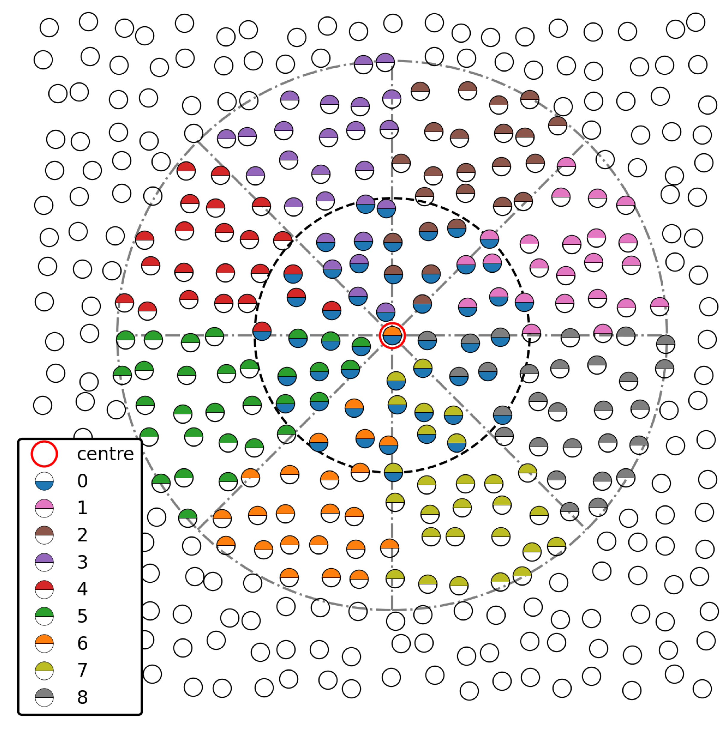
For each i-th particle, several candidate stencils for the reconstruction are initially considered, each of them composed by a subset of the particles in the neighbourhood. Figure 1 shows a sketch of the candidate stencils for a sample randomized 2D particle distribution. The so-called central stencil is composed by all the particles at distance lower or equal to the length of the kernel support. On the other hand, there are several lateral one-sided stencils, all of them composed by particles at distance lower or equal to the double of the length of the kernel support. In 2D, there are 8 lateral one-sided stencils: a neighbouring j-th particle belongs to the s stencil () when the polar coordinate of the vector fulfils the expression:
It should be noted that the particles belonging to the central stencil are also part of one of the lateral one-sided stencils. In general, SPH particles move in time; hence, at each time step, the particles that form a given candidate stencil change.
For each candidate stencil, a (local) candidate polynomial reconstruction is built. Differently from what was done in [31], a corrected SPH interpolation has been used in the present work to compute the polynomial coefficients, as will be explained in Section 2.4.
In this stencil-adaptive WENO method, the final reconstructed polynomial is a weighted average of all the candidate stencil polynomials,
To determine the weights that appear in (13), the following unnormalized weights are computed first:
where for the one-sided lateral stencils (), and for the central stencil; is introduced to avoid dividing by zero (valid values are and for single and double precision, respectively); and is an indicator of the smoothness of the candidate polynomial based on the values of its coefficients:
It should be noted that Equation (14) favours the contribution of the central polynomial candidate, and effectively filters out the contributions of polynomial candidates that are oscillatory. Finally, a normalization of the weights is done via the expression:
Once a local polynomial reconstruction is defined for every particle, the left state of the Riemann problem for the pair is obtained from the reconstruction local to particle i, and the right state is obtained from the reconstruction local to particle j.
2.4. Corrected SPH Estimation of Derivatives
In this work, the consistency correction proposed in [22] is applied to compute the coefficients of the polynomials involved in the WENO reconstruction. For completeness, the following paragraphs explain the process to restore consistency in SPH.
The objective is to use SPH summations to compute at the location of a given particle i the values of a function, , and its derivatives of successive order, , , …(the indexes , , …traverse the different dimension variables of the space). For convenience, a Taylor expansion of f around particle i is used to express the value of f at the neighbouring particle j,
where represents the component of the position vector of particle i. It should be noted that the Einstein summation convention is adopted.
Without loss of generality, it may be assumed that the objective is to achieve first order consistency (or second order accuracy) in the SPH estimation. Then, all the terms in Equation (17) containing second or higher order derivatives can be neglected, and the remaining unknowns are and the first order derivatives . Multiplying the resulting expression by the product of the volume of particle j times the value of the smoothing kernel, , and summing for all the neighbouring particles j, a first equation is obtained:
Taking similar actions but using instead the first order derivatives of the smoothing kernel, , leads to analogous equations (as many as the number of dimensions of the space):
Equations (18) and (19) form a linear system that can be solved, for instance, with an LU decomposition [44].
Please note that, if achieving a higher order of consistency is required, then higher order derivatives of the kernel function can be considered in the Taylor expansion of Equation (17), and this process can be readily generalised.
Generation of polynomials for the Weighted Essentially Non-Oscillatory Reconstruction
In the WENO reconstruction it is necessary to estimate the polynomial coefficients that appear in Equation (11). This is a computationally expensive process that needs to be done for each of the candidate stencils (e.g., nine times in a 2D space). Avesani et al. [31] use a least-squares fit to carry out this task. In the present work we propose to use a corrected SPH interpolation described in Section 2.4 for the estimation of the polynomial coefficients (equivalent to the estimation of the reconstructed function derivatives by virtue of a Taylor expansion). The benefits in terms of computational efficiency and accuracy will be supported with data subsequently.
3. Results and Discussion
3.1. Moving Least-Squares vs. Corrected SPH Interpolation for the Generation of Reconstruction Polynomials
This section focuses on the comparison of the computational performance and the accuracy of an MLS fit used in [31] and the corrected SPH interpolation described in Section 2.4 to compute the coefficients of the polynomial reconstruction (11). With this aim, both methods will be used to reconstruct the following 2D scalar function:
in the squared domain with periodic boundary conditions. The (exact) value of f is known at the particle positions, and two different particle arrangements have been adopted: (a) particles distributed in the vertices of a Cartesian grid with horizontal and vertical spacing equal to a certain length, , and (b) particles distributed randomly by applying a uniformly distributed random perturbation (of maximum length , with ) to the x and y coordinates of an initial Cartesian grid configuration. For each particle i, a second order polynomial reconstruction:
is produced from the data of the particles in a neighbourhood of radius 4 times . To evaluate the reconstructions, a Cartesian reconstruction grid is created initially superimposed to the above-mentioned particle arrangement (a), then the grid is shifted by the distance both in positive x and y directions. For the computation of the error, each reconstructing polynomial will be evaluated at the reconstruction grid point placed closest to the centre of the reconstruction, and compared to the exact value of f. Finally, for the corrected SPH interpolations, the popular cubic spline kernel is used [37], with a smoothing length .
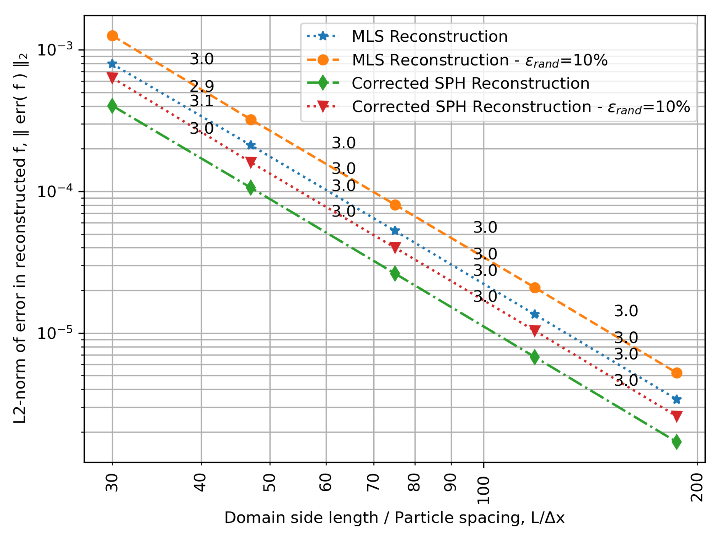
Figure 2 shows the convergence of the L2 norm of the error in the reconstruction of Equation (20) for the MLS and for the corrected SPH interpolation methods (annotations of the order of convergence are also included). The MLS reconstructions have been computed via a Singular Value Decomposition (SVD) algorithm (see, e.g., chapter 15 in [45] for details). Both above-mentioned uniform and randomized particle distributions have been used. A third order convergence rate is achieved as one would expect from the second order approximation of (21). However, in both particle arrangements, the accuracy of the reconstruction when using corrected SPH interpolations is higher for a given resolution.
More importantly, the average measured computational cost for the method using the corrected SPH interpolation is 3.5 smaller than for MLS. Considering that the WENO method requires one of these polynomial reconstructions per candidate stencil (e.g., 9 polynomials in a 2D case), it is expected that the associated speed-up in the complete SPH scheme will be remarkable.
3.2. Weakly Compressible 2D Vortex
A weakly compressible 2D vortex, as described in [46], has been chosen for the evaluation of the SPH scheme used in this work. This is an inviscid, stationary problem that has circular streamlines. Interestingly, an analytical solution given by the following expressions is available:
where and have already been defined in (7), is the asymptotic value of density, and marks the position where the (tangential) velocity is maximal. Please note that the analytical solution depends only on the radial distance r. The actual values of these parameters used in this work are: = 1.0 m/s, = 1.0 kg/m2, = 1.01 kg/m2, and = 0.1 m. The size of the circular simulation domain is R = 0.7 m. There are several reasons to select this test case for the preliminary studies of the present WENO-SPH scheme. Firstly, boundary conditions can be easily enforced with the appropriate number of rows of dummy particles around the simulation domain (where the analytical solution is imposed). This allows to avoid the situation where some of the candidate reconstruction stencils lack of sufficient neighbouring particles to build the corresponding polynomials. On the other hand, the test case is challenging as in general vortices are difficult to capture for Lagrangian particle methods.
For convenience, all the simulation results are expressed in non-dimensional variables, marked by a hat symbol (⌃). These variables are defined as follows:
Please note that the non-dimensional time above can be interpreted as the angle (in radians) that the radius vector of the fastest particles (i.e., the ones at ) traverses in that time.
Regarding the SPH scheme, second order polynomials are used for the WENO reconstruction. The kernel is a cubic spline (see definition in [37]), with a smoothing length for all the simulations. The CFL number has been set equal to 0.2. Unless explicitly stated otherwise, the simulations are performed adopting a Lagrangian transport velocity ().
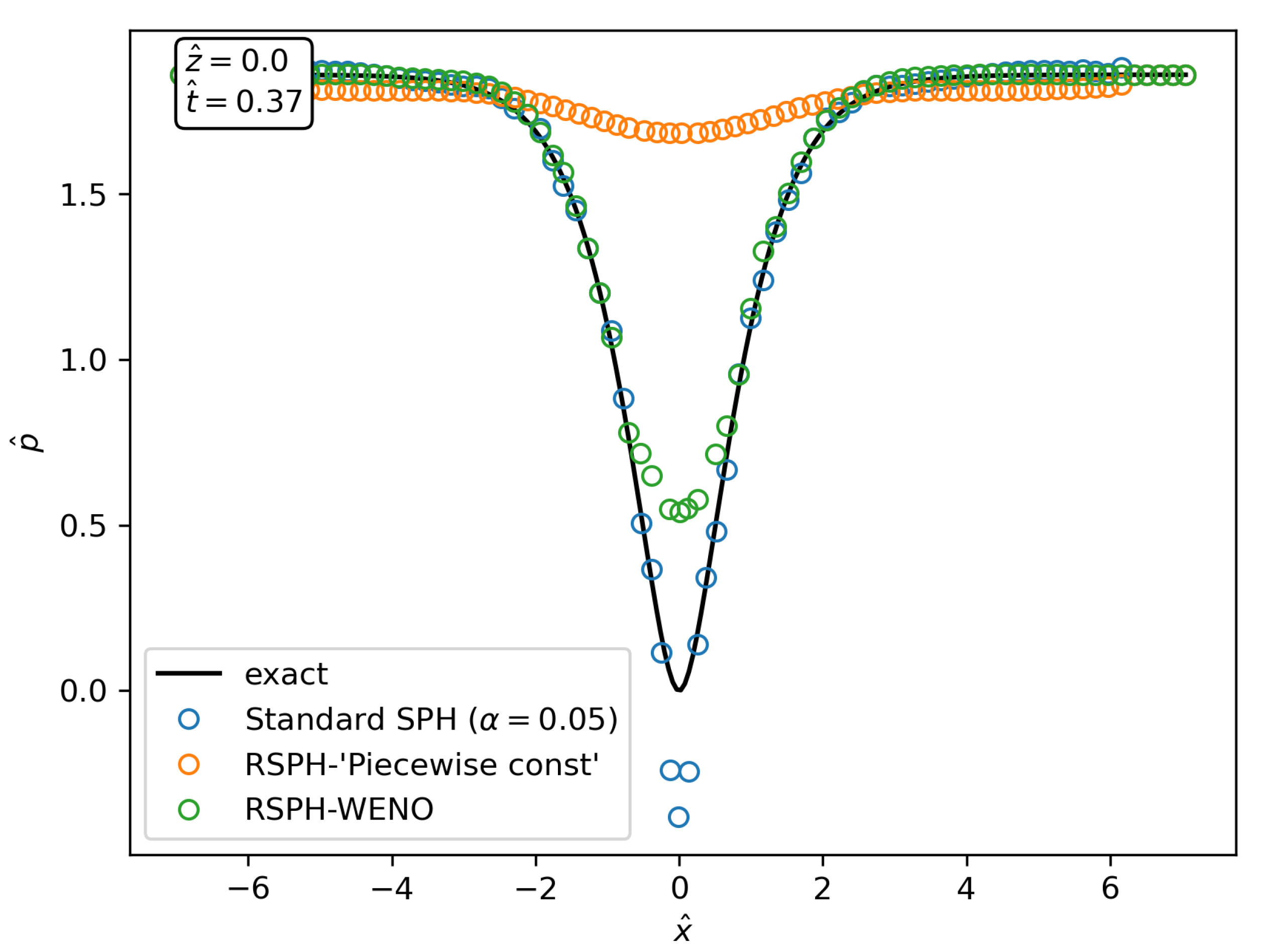
Figure 3 shows the pressure distribution along the line and at time , computed with a standard SPH scheme with artificial viscosity (see details in [37]), and two Riemann-based SPH (RSPH) schemes: one with a piece-wise constant reconstruction and the other one with the polynomial WENO reconstruction. The resolution of the simulations is , and the exact (stationary) solution is provided for comparison. The value chosen for the artificial viscosity coefficient () is typical of applications in the hydraulics field. Please note that the selected physical time corresponds to a sufficiently early instant in the simulation which guarantees that the fluid has not experienced large deformations yet. This is needed to obtain meaningful results in Lagrangian simulations without a dedicated treatment for irregular particle distributions. It may be seen that the artificial viscosity used in the standard SPH scheme introduces a spurious spike around . On the other hand, the RSPH scheme is very good at stabilizing the results without spurious effects. However, the unavoidable numerical diffusion that it introduces is too large when using the piece-wise constant reconstruction, affecting the accuracy of the solution. Finally, the high-order reconstruction in the RSPH-WENO scheme largely improves its accuracy.
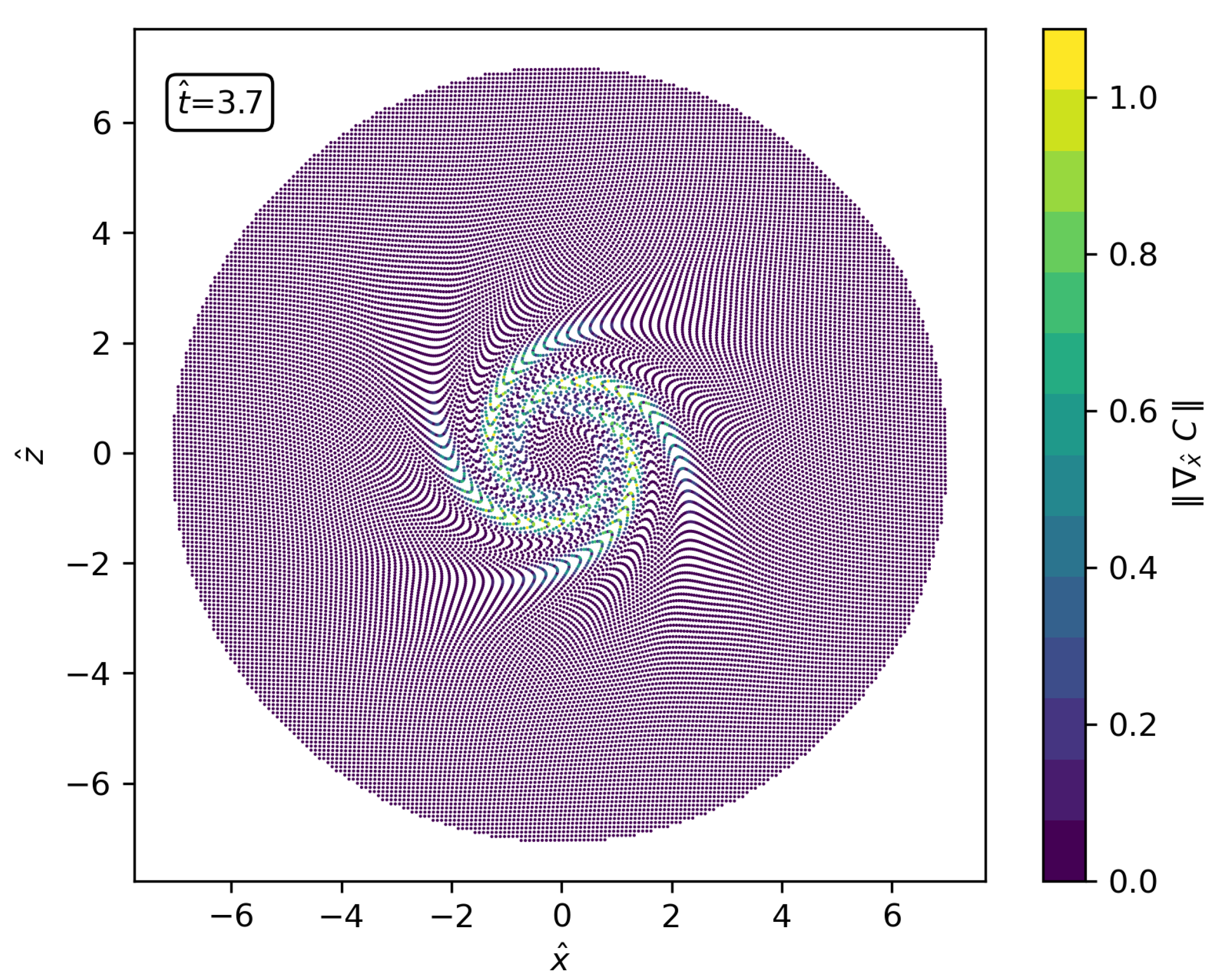
Figure 4 shows the distribution of particles of the 2D vortex simulation (with the RSPH-WENO scheme) at a later physical time, , with the magnitude of the gradient of partition of unity superimposed:
In this plot, the resolution is . The high-order spatial reconstruction makes the particles move accurately along their Lagrangian trajectories which in its turn leads to anisotropic particle distributions. An immediate consequence is the (local) increase of the gradient of partition of unity which translates into low accuracy of the standard SPH approximations of divergence operators used in Equations (5) and (6).
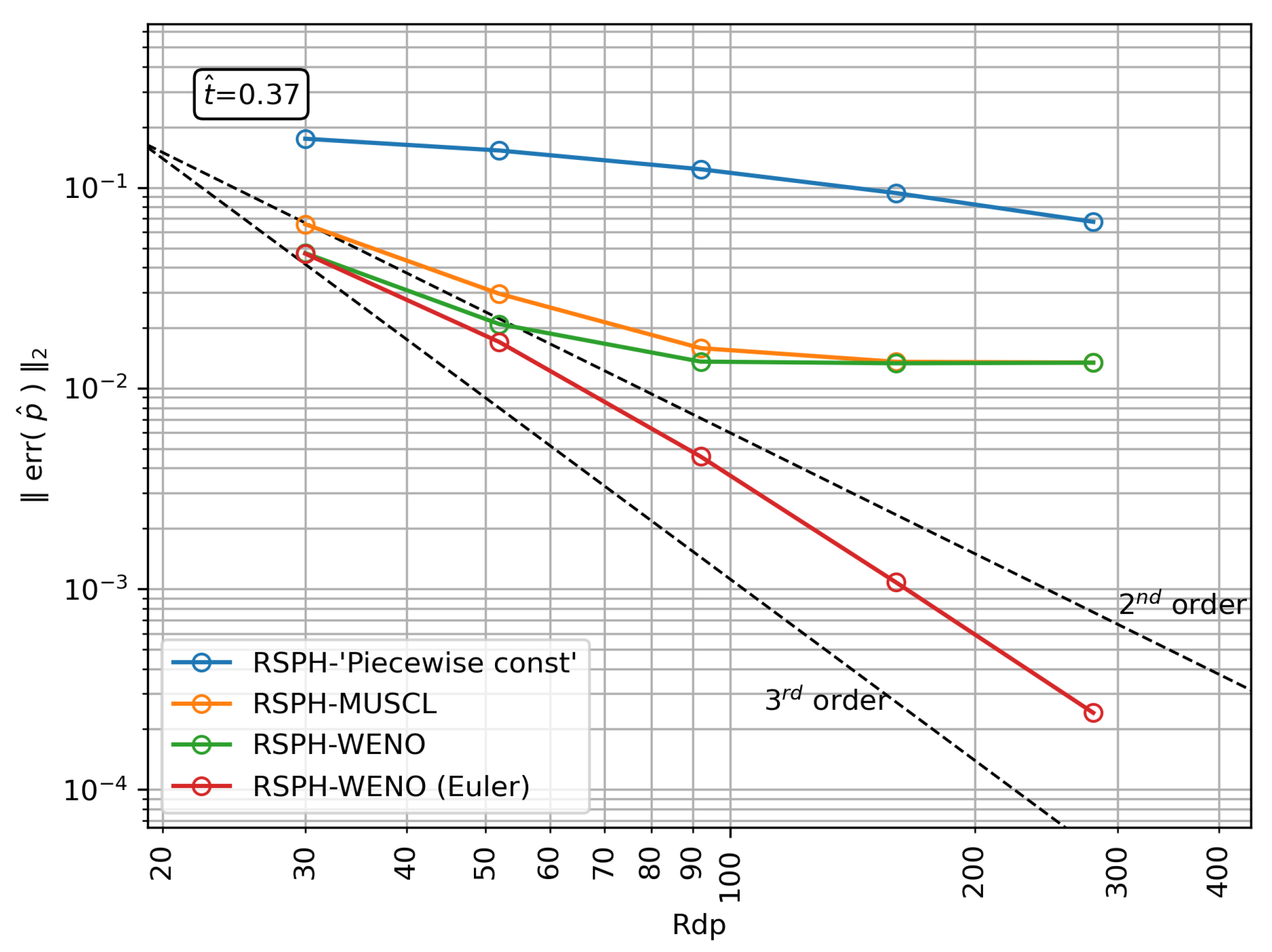
Aiming at further comparing the different schemes herein adopted, Figure 5 shows the convergence of the L2 norm of the pressure error at for the following five different RSPH schemes:
- RSPH with a piece-wise constant reconstruction. This is the less accurate scheme due to the very large diffusion introduced by the Riemann problem with a trivial reconstruction.
- RSPH with a MUSCL reconstruction. Uses linear reconstructions based on gradients estimated by standard SPH operators, with slope limiters (to prevent oscillatory fields) as first depicted by [30]. The MUSCL reconstruction improves the accuracy of the scheme to the point that anisotropic distributions (like the ones displayed in Figure 4 for the RSPH-WENO scheme) appear, especially for high resolutions. The result is an increase in the discretization error that saturates the decrease in the global error.
- RSPH with WENO reconstruction: The high-order spatial reconstruction further improves the accuracy of the trajectories described by the particles which, in conjunction with the usage of standard divergence SPH operators in Equations (5) and (6), ruins the beneficial effect of the high-order reconstruction.
- RSPH with WENO reconstruction and Eulerian transport. In these simulations, particles remain fixed on the vertices of a Cartesian grid (). Hence, the gradient of partition of unity is exactly zero in the whole field, unleashing the full potential of the WENO reconstruction to reach a maximum convergence rate of ∼2.7. Considering that the theoretical convergence for the second order reconstructing polynomials used is third order, this result suggests that the overall convergence of the scheme is guided by the order of the WENO polynomials.
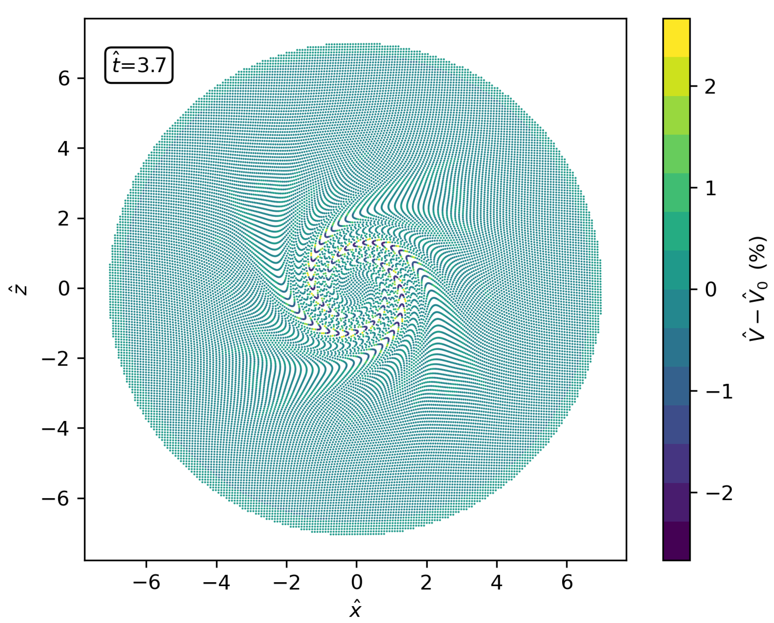
Figure 6 displays the distribution of particles of the 2D vortex simulation at with the field of unitary volume variation superimposed
computed by the RSPH-WENO scheme. In this plot, the resolution is . It may be seen that the algorithm keeps volume variations small, below a 3% (in absolute value).
Finally, Table 1 details the approximate computational time for two different Riemann-based SPH schemes relative to that of a standard SPH scheme with artificial viscosity (see details in [37]), for a given resolution. The large number of candidate polynomials reconstructions in WENO makes this method notably more expensive. However, with the high-order method the same level of accuracy can be reached with a lower resolution, as it may be seen in Table 2 that compares the performance of standard SPH and the Riemann-based SPH scheme with WENO reconstruction. With the much lower resolution required by the WENO SPH scheme, a 25 percent speed-up is actually achieved. Note that the value of the artificial viscosity coefficient has been chosen aiming at obtaining a similar amount of numerical diffusion (i.e., a similar depth of the central area in Figure 3) compared to that of the solution computed with the WENO SPH scheme. However, it is not possible to match exactly both the numerical diffusion and the L2 norm of the pressure error so a compromise value has been adopted.
4. Conclusions
In this paper, the convergence properties of a polynomial WENO ALE-SPH scheme have been investigated. For the case of a weakly compressible 2D vortex, it has been demonstrated first that the accuracy of the Lagrangian trajectories of the SPH particles improves with the WENO reconstruction, to the point that anisotropic particle configurations easily form. As a result, the truncation error in the discrete SPH operators becomes dominant and produces the saturation of the global error with increasing resolutions. It has also been shown that, with the aid of a Eulerian simulation with particles fixed on the vertices of a Cartesian grid, this truncation error can be eliminated, obtaining high order convergence (∼3). More importantly, the fact that the order of convergence achieved is very close to the order of the adopted WENO polynomials suggests that this type of schemes is a viable path to reach high order convergence in SPH (which is one of the main goals of the present work).
Furthermore, a novel efficient procedure based on a corrected SPH interpolation for the estimation of the coefficients of the underlying WENO (candidate) polynomial reconstructions has been proposed. Compared to the MLS approach used in [31], this method not only increases the accuracy of the results but brings a speed-up in computational time by a factor of 3.5.
In connection with the convergence analysis of the WENO SPH scheme, and thanks to the ALE framework of the SPH formulation used in this work, it should be noted that it is also possible to tackle the issue of the anisotropic particle distributions by means of particle regularisation techniques (as firstly proposed by [47]) that perturb the Lagrangian transport velocities with a small shifting velocity field that keeps the particle distribution regular. Contrary to the Eulerian simulation performed in the present work, this approach would allow to (approximately) keep the Lagrangian nature that has characterized so far the SPH method (very useful, e.g., in problems with free surfaces). Another interest of this technique in an ALE framework (which is left for future research) is that both conservation and consistency of the scheme would be kept.
The formulation of general boundary conditions (e.g., walls and free surfaces) in the framework of the polynomial WENO-SPH scheme has not been tackled in the present work. The challenge lies in the potential incompleteness of some of the candidate WENO reconstruction stencils when boundaries are present. The appropriate treatment that would keep high order convergence of the numerical solution also close to boundaries remains to be investigated.
Author Contributions
Conceptualization, R.A., R.V., D.A., M.R. (Maurizio Righetti) and M.R. (Massimiliano Renzi); methodology, R.A.; software, R.A.; validation, R.A., R.V. and D.A.; formal analysis, R.A.; investigation, R.A.; resources, M.R. (Maurizio Righetti) and M.R. (Massimiliano Renzi); data curation, R.A.; writing—original draft preparation, R.A.; writing—review and editing, R.V., D.A., M.R. (Maurizio Righetti) and M.R. (Massimiliano Renzi); visualization, R.A.; supervision, R.V., D.A., M.R. (Maurizio Righetti) and M.R. (Massimiliano Renzi); project administration, M.R. (Maurizio Righetti) and M.R. (Massimiliano Renzi); funding acquisition, M.R. (Maurizio Righetti). All authors have read and agreed to the published version of the manuscript.
Funding
The APC was funded by the Open Access Publishing Fund of the Free University of Bozen-Bolzano.
Acknowledgments
R. Antona, D. Avesani, M. Righetti and M. Renzi acknowledge funding from the EFRE-FESR project “TURB HYDRO, Hydrokinetic turbines, optimization for sustainable production” (ERDF 2018-2021, CUP: I56C18000040009).
Conflicts of Interest
The authors declare no conflict of interest.
Abbreviations
The following abbreviations are used in this manuscript:
| SPH | Smoothed Particle Hydrodynamics |
| WEC | Wave Energy Converters |
| LES | Large Eddy Simulation |
| SPHERIC | SPH rEsearch and engineeRing |
| MLS | Moving least-squares |
| ALE | Arbitrary Lagrangian–Eulerian |
| WENO | Weighted Essentially Non-Oscillatory |
| ADER | Arbitrary DERivative |
| MOOD | Multi-dimensional Optimal Order Detection |
| LABFM | Local Anisotropic Basis Function Method |
| GPU | Graphics Processing Unit |
| CFL | Courant–Friedrichs–Lewy |
| RSPH | Riemann-based SPH |
References
- Gingold, R.A.; Monaghan, J.J. Smoothed particle hydrodynamics: Theory and application to non-spherical stars. Mon. Not. R. Astron. Soc. 1977, 181, 375–389. [Google Scholar] [CrossRef]
- Lucy, L.B. A numerical approach to the testing of the fission hypothesis. Astron. J. 1977, 82, 1013–1024. [Google Scholar] [CrossRef]
- Monaghan, J.J. Simulating Free Surface Flows with SPH. J. Comput. Phys. 1994, 110, 399–406. [Google Scholar] [CrossRef]
- Shadloo, M.; Oger, G.; Le Touzé, D. Smoothed particle hydrodynamics method for fluid flows, towards industrial applications: Motivations, current state, and challenges. Comput. Fluids 2016, 136, 11–34. [Google Scholar] [CrossRef]
- Violeau, D. Fluid Mechanics and the SPH Method: Theory and Applications; Oxford University Press: Oxford, UK, 2012. [Google Scholar] [CrossRef]
- Lind, S.J.; Rogers, B.D.; Stansby, P.K. Review of smoothed particle hydrodynamics: Towards converged Lagrangian flow modelling. Proc. R. Soc. A 2020, 476. [Google Scholar] [CrossRef]
- Bottelli, D.N. Application of Smoothed Particle Hydrodynamics (SPH) for preliminary hydraulic design of Water-WasterWater Works. In Proceedings of the 14th International SPHERIC Workshop, Exeter, UK, 25–27 June 2019. [Google Scholar]
- Rentschler, M.; Marongiu, J.C.; Neuhauser, M.; Parkinson, E. Overview of SPH-ALE applications for hydraulic turbines in ANDRITZ Hydro. J. Hydrodyn. 2018, 30, 114–121. [Google Scholar] [CrossRef]
- Novak, G.; Domínguez, J.M.; Tafuni, A.; Silva, A.T.; Pengal, P.; Četina, M.; Žagar, D. 3-D Numerical Study of a Bottom Ramp Fish Passage Using Smoothed Particle Hydrodynamics. Water 2021, 13, 1595. [Google Scholar] [CrossRef]
- O’Connor, J.; Rogers, B.D. A fluid–structure interaction model for free-surface flows and flexible structures using smoothed particle hydrodynamics on a GPU. J. Fluids Struct. 2021, 104, 103312. [Google Scholar] [CrossRef]
- Green, M.D.; Zhou, Y.; Dominguez, J.M.; Gesteira, M.G.; Peiró, J. Smooth particle hydrodynamics simulations of long-duration violent three-dimensional sloshing in tanks. Ocean Eng. 2021, 229, 108925. [Google Scholar] [CrossRef]
- Quartier, N.; Ropero-Giralda, P.; Domínguez, J.M.; Stratigaki, V.; Troch, P. Influence of the Drag Force on the Average Absorbed Power of Heaving Wave Energy Converters Using Smoothed Particle Hydrodynamics. Water 2021, 13, 384. [Google Scholar] [CrossRef]
- Altomare, C.; Tafuni, A.; Domínguez, J.M.; Crespo, A.J.C.; Gironella, X.; Sospedra, J. SPH Simulations of Real Sea Waves Impacting a Large-Scale Structure. J. Mar. Sci. Eng. 2020, 8, 826. [Google Scholar] [CrossRef]
- Di Mascio, A.; Antuono, M.; Colagrossi, A.; Marrone, S. Smoothed particle hydrodynamics method from a large eddy simulation perspective. Phys. Fluids 2017, 29, 035102. [Google Scholar] [CrossRef]
- Antuono, M.; Marrone, S.; Di Mascio, A.; Colagrossi, A. Smoothed particle hydrodynamics method from a large eddy simulation perspective. Generalization to a quasi-Lagrangian model. Phys. Fluids 2021, 33, 15102. [Google Scholar] [CrossRef]
- Vacondio, R.; Altomare, C.; De Leffe, M.; Hu, X.; Le Touzé, D.; Lind, S.; Marongiu, J.C.; Marrone, S.; Rogers, B.D.; Souto-Iglesias, A. Grand challenges for Smoothed Particle Hydrodynamics numerical schemes. Comput. Part. Mech. 2021, 8, 575–588. [Google Scholar] [CrossRef]
- Monaghan, J.J. Smoothed Particle Hydrodynamics. Annu. Rev. Astron. Astrophys. 1992, 30, 543–574. [Google Scholar] [CrossRef]
- Quinlan, N.J.; Basa, M.; Lastiwka, M. Truncation error in mesh-free particle methods. Int. J. Numer. Methods Eng. 2006, 66, 2064–2085. [Google Scholar] [CrossRef]
- Shepard, D. A two-dimensional interpolation function for irregularly-spaced data. In Proceedings of the 1968 23rd ACM National Conference, New York, NY, USA, 27–29 August 1968; ACM Press: New York, NY, USA, 1968; pp. 517–524. [Google Scholar] [CrossRef]
- Randles, P.W.; Libersky, L.D. Smoothed Particle Hydrodynamics: Some recent improvements and applications. Comput. Methods Appl. Mech. Eng. 1996, 139, 375–408. [Google Scholar] [CrossRef]
- Bonet, J.; Kulasegaram, S. Correction and stabilization of smooth particle hydrodynamics methods with applications in metal forming simulations. Int. J. Numer. Methods Eng. 2000, 47, 1189–1214. [Google Scholar] [CrossRef]
- Liu, M.B.; Liu, G.R. Restoring particle consistency in smoothed particle hydrodynamics. Appl. Numer. Math. 2006, 56, 19–36. [Google Scholar] [CrossRef]
- Sibilla, S. An algorithm to improve consistency in Smoothed Particle Hydrodynamics. Comput. Fluids 2015, 118, 148–158. [Google Scholar] [CrossRef]
- Dilts, G.A. Moving least-squares-particle hydrodynamics I. Consistency and stability. Int. J. Numer. Methods Eng. 1999, 44, 1115–1155. [Google Scholar] [CrossRef]
- Chaniotis, A.K.; Poulikakos, D.; Koumoutsakos, P. Remeshed smoothed particle hydrodynamics for the simulation of viscous and heat conducting flows. J. Comput. Phys. 2002, 182, 67–90. [Google Scholar] [CrossRef] [Green Version]
- Monaghan, J.J. On the Problem of Penetration in Particle Methods. J. Comput. Phys. 1989, 82, 1–15. [Google Scholar] [CrossRef]
- Lind, S.J.; Xu, R.; Stansby, P.K.; Rogers, B.D. Incompressible smoothed particle hydrodynamics for free-surface flows: A generalised diffusion-based algorithm for stability and validations for impulsive flows and propagating waves. J. Comput. Phys. 2012, 231, 1499–1523. [Google Scholar] [CrossRef]
- Lind, S.; Stansby, P. High-order Eulerian incompressible smoothed particle hydrodynamics with transition to Lagrangian free-surface motion. J. Comput. Phys. 2016, 326, 290–311. [Google Scholar] [CrossRef]
- Fourtakas, G.; Vacondio, R.; Rogers, B.D. An arbitrary Lagrangian–Eulerian weakly compressible SPH formulation by means of iterative diffusion-based particle shifting. In Proceedings of the 14th International SPHERIC Workshop, University of, Exeter, Exeter, UK, 25–27 June 2019. [Google Scholar]
- Vila, J.P. On particle weighted methods and Smooth Particle Hydrodynamics. Math. Model. Methods Appl. Sci. 1999, 09, 161–209. [Google Scholar] [CrossRef]
- Avesani, D.; Dumbser, M.; Bellin, A. A new class of Moving-Least-Squares WENO–SPH schemes. J. Comput. Phys. 2014, 270, 278–299. [Google Scholar] [CrossRef]
- Avesani, D.; Dumbser, M.; Vacondio, R.; Righetti, M. An alternative SPH formulation: ADER-WENO-SPH. Comput. Methods Appl. Mech. Eng. 2021, 382, 113871. [Google Scholar] [CrossRef]
- Vergnaud, A.; Oger, G.; Le Touzé, D. A higher order SPH scheme based on WENO reconstructions for two-dimensional problems. In Proceedings of the 14th International SPHERIC Workshop, University of, Exeter, Exeter, UK, 25–27 June 2019. [Google Scholar]
- Zhang, C.; Xiang, G.M.; Wang, B.; Hu, X.Y.; Adams, N.A. A weakly compressible SPH method with WENO reconstruction. J. Comput. Phys. 2019, 392, 1–18. [Google Scholar] [CrossRef]
- Eirís, A.; Ramírez, L.; Fernández-Fidalgo, J.; Couceiro, I.; Nogueira, X. SPH-ALE Scheme for Weakly Compressible Viscous Flow with a Posteriori Stabilization. Water 2021, 13, 245. [Google Scholar] [CrossRef]
- Nasar, A.M.; Fourtakas, G.; Lind, S.J.; Rogers, B.D.; Stansby, P.K.; King, J.R. High-order velocity and pressure wall boundary conditions in Eulerian incompressible SPH. J. Comput. Phys. 2021, 434, 109793. [Google Scholar] [CrossRef]
- Domínguez, J.M.; Fourtakas, G.; Altomare, C.; Canelas, R.B.; Tafuni, A.; García-Feal, O.; Martínez-Estévez, I.; Mokos, A.; Vacondio, R.; Crespo, A.J.C.; et al. DualSPHysics: From fluid dynamics to multiphysics problems. Comput. Part. Mech. 2021. [Google Scholar] [CrossRef]
- English, A.; Domínguez, J.M.; Vacondio, R.; Crespo, A.J.C.; Stansby, P.K.; Lind, S.J.; Chiapponi, L.; Gómez-Gesteira, M. Modified dynamic boundary conditions (mDBC) for general-purpose smoothed particle hydrodynamics (SPH): Application to tank sloshing, dam break and fish pass problems. Comput. Part. Mech. 2021. [Google Scholar] [CrossRef]
- King, J.R.; Lind, S.J.; Nasar, A.M. High order difference schemes using the local anisotropic basis function method. J. Comput. Phys. 2020, 415, 109549. [Google Scholar] [CrossRef]
- Batchelor, G.K. An Introduction to Fluid Dynamics; Cambridge University Press: Cambridge, UK, 2000. [Google Scholar] [CrossRef]
- Liu, M.B.; Liu, G.R. Smoothed Particle Hydrodynamics (SPH): An Overview and Recent Developments. Arch. Comput. Methods Eng. 2010, 17, 25–76. [Google Scholar] [CrossRef] [Green Version]
- Avesani, D.; Herrera, P.; Chiogna, G.; Bellin, A.; Dumbser, M. Smooth Particle Hydrodynamics with nonlinear Moving-Least-Squares WENO reconstruction to model anisotropic dispersion in porous media. Adv. Water Resour. 2015, 80, 43–59. [Google Scholar] [CrossRef]
- Avesani, D.; Dumbser, M.; Chiogna, G.; Bellin, A. An alternative smooth particle hydrodynamics formulation to simulate chemotaxis in porous media. J. Math. Biol. 2017, 74, 1037–1058. [Google Scholar] [CrossRef] [Green Version]
- Bunch, J.R.; Hopcroft, J.E. Triangular Factorization and Inversion by Fast Matrix Multiplication. Math. Comput. 1974, 28, 231–236. [Google Scholar] [CrossRef]
- Press, W.H.; Teukolsky, S.A.; Vetterling, W.T.; Flannery, B.P. Numerical Recipes in Fortran, 2nd ed.; Cambridge University Press: Cambridge, UK, 1992. [Google Scholar]
- Vacondio, R.; Rogers, B. Consistent Iterative shifting for SPH methods. In Proceedings of the 12th International SPHERIC Workshop, Universidade de Vigo, Ourense, Spain, 13–15 June 2017. [Google Scholar]
- Oger, G.; Marrone, S.; Le Touzé, D.; de Leffe, M. SPH accuracy improvement through the combination of a quasi-Lagrangian shifting transport velocity and consistent ALE formalisms. J. Comput. Phys. 2016, 313, 76–98. [Google Scholar] [CrossRef]
Figure 1.
Sketch of the central and the one-sided lateral stencils for a sample randomized 2D particle distribution.
Figure 1.
Sketch of the central and the one-sided lateral stencils for a sample randomized 2D particle distribution.

Figure 2.
Convergence of the L2 norm of the error in the reconstruction of Equation (20) in the squared domain with side length L = 2 m. Results are displayed for the MLS and for the corrected SPH interpolation methods (with a smoothing length ), as well as for both uniform and randomized particle distributions. Annotations of the order of convergence are included.

Figure 3.
Pressure distribution of the 2D vortex along the line and at time , computed with three different schemes: standard SPH with artificial viscosity (), RSPH with a piece-wise constant reconstruction, and RSPH with a WENO reconstruction. The resolution is .
Figure 3.
Pressure distribution of the 2D vortex along the line and at time , computed with three different schemes: standard SPH with artificial viscosity (), RSPH with a piece-wise constant reconstruction, and RSPH with a WENO reconstruction. The resolution is .

Figure 4.
Distribution of particles of the 2D vortex simulation (with the RSPH-WENO scheme) at , with the magnitude of the gradient of partition of unity superimposed. The resolution is .
Figure 4.
Distribution of particles of the 2D vortex simulation (with the RSPH-WENO scheme) at , with the magnitude of the gradient of partition of unity superimposed. The resolution is .

Figure 5.
Convergence of the L2 norm of the 2D vortex pressure error at (the resolution is expressed as the ratio between the domain radius and the particle spacing, Rdp) for five different RSPH schemes.
Figure 5.
Convergence of the L2 norm of the 2D vortex pressure error at (the resolution is expressed as the ratio between the domain radius and the particle spacing, Rdp) for five different RSPH schemes.

Figure 6.
Distribution of particles at for the 2D vortex case, with the field of unitary volume variation superimposed, computed by the RSPH-WENO scheme. The resolution is .
Figure 6.
Distribution of particles at for the 2D vortex case, with the field of unitary volume variation superimposed, computed by the RSPH-WENO scheme. The resolution is .


Table 1.
Computational time of Riemann-based schemes relative to a standard SPH scheme (for a given resolution).
Table 1.
Computational time of Riemann-based schemes relative to a standard SPH scheme (for a given resolution).
| Riemann-Based Scheme | CPU Time / CPU Time Standard SPH |
|---|---|
| MUSCL | 2.5 |
| WENO | 10.9 |
Table 2.
Performance comparison of standard SPH and Riemann-based with WENO reconstruction SPH, for the 2D vortex case. Values of the L2 norm of the pressure error at are provided.
Table 2.
Performance comparison of standard SPH and Riemann-based with WENO reconstruction SPH, for the 2D vortex case. Values of the L2 norm of the pressure error at are provided.
| SPH Scheme | CPU time / CPU Time Standard SPH | ||
|---|---|---|---|
| Standard SPH () | 160 | 0.020532 | 1 |
| WENO-RSPH | 52 | 0.020878 | 0.75 |
Publisher’s Note: MDPI stays neutral with regard to jurisdictional claims in published maps and institutional affiliations. |
© 2021 by the authors. Licensee MDPI, Basel, Switzerland. This article is an open access article distributed under the terms and conditions of the Creative Commons Attribution (CC BY) license (https://creativecommons.org/licenses/by/4.0/).
Share and Cite
MDPI and ACS Style
Antona, R.; Vacondio, R.; Avesani, D.; Righetti, M.; Renzi, M. Towards a High Order Convergent ALE-SPH Scheme with Efficient WENO Spatial Reconstruction. Water 2021, 13, 2432. https://doi.org/10.3390/w13172432
AMA Style
Antona R, Vacondio R, Avesani D, Righetti M, Renzi M. Towards a High Order Convergent ALE-SPH Scheme with Efficient WENO Spatial Reconstruction. Water. 2021; 13(17):2432. https://doi.org/10.3390/w13172432
Chicago/Turabian StyleAntona, Rubén, Renato Vacondio, Diego Avesani, Maurizio Righetti, and Massimiliano Renzi. 2021. "Towards a High Order Convergent ALE-SPH Scheme with Efficient WENO Spatial Reconstruction" Water 13, no. 17: 2432. https://doi.org/10.3390/w13172432
Note that from the first issue of 2016, this journal uses article numbers instead of page numbers. See further details here.