
Aquifer Parameters Estimation from Natural Groundwater Level Fluctuations at the Mexican Wine-Producing Region Guadalupe Valley, BC

 , , ,
, , ,
Abstract
:1. Introduction
2. Methods
2.1. Aquifer Response to Earth and Atmospheric Tides
2.2. Groundwater-Level Response to Atmospheric Pressure
2.3. Groundwater-Level Response to Solid Earth Tide
2.4. Aquifer Parameters Estimation
3. Study Area and Database
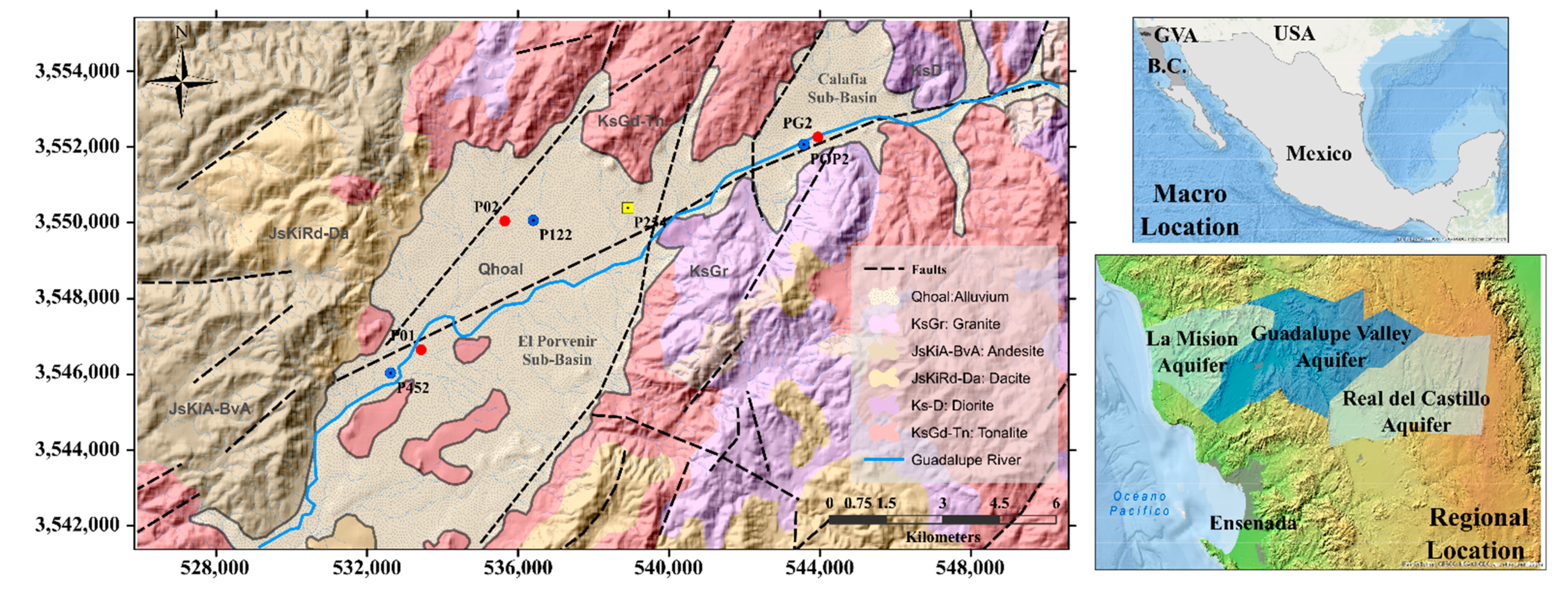
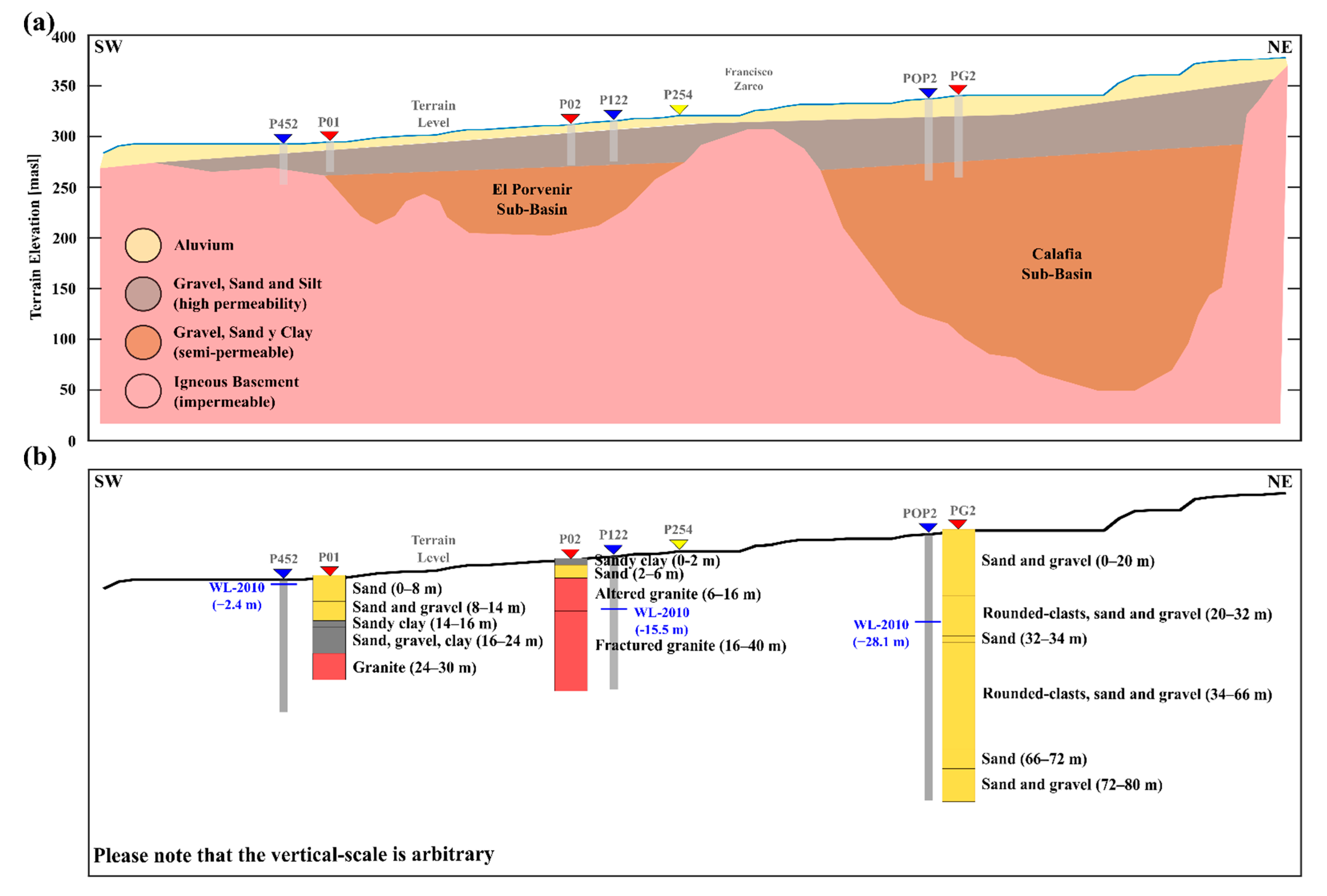
3.1. Study Area
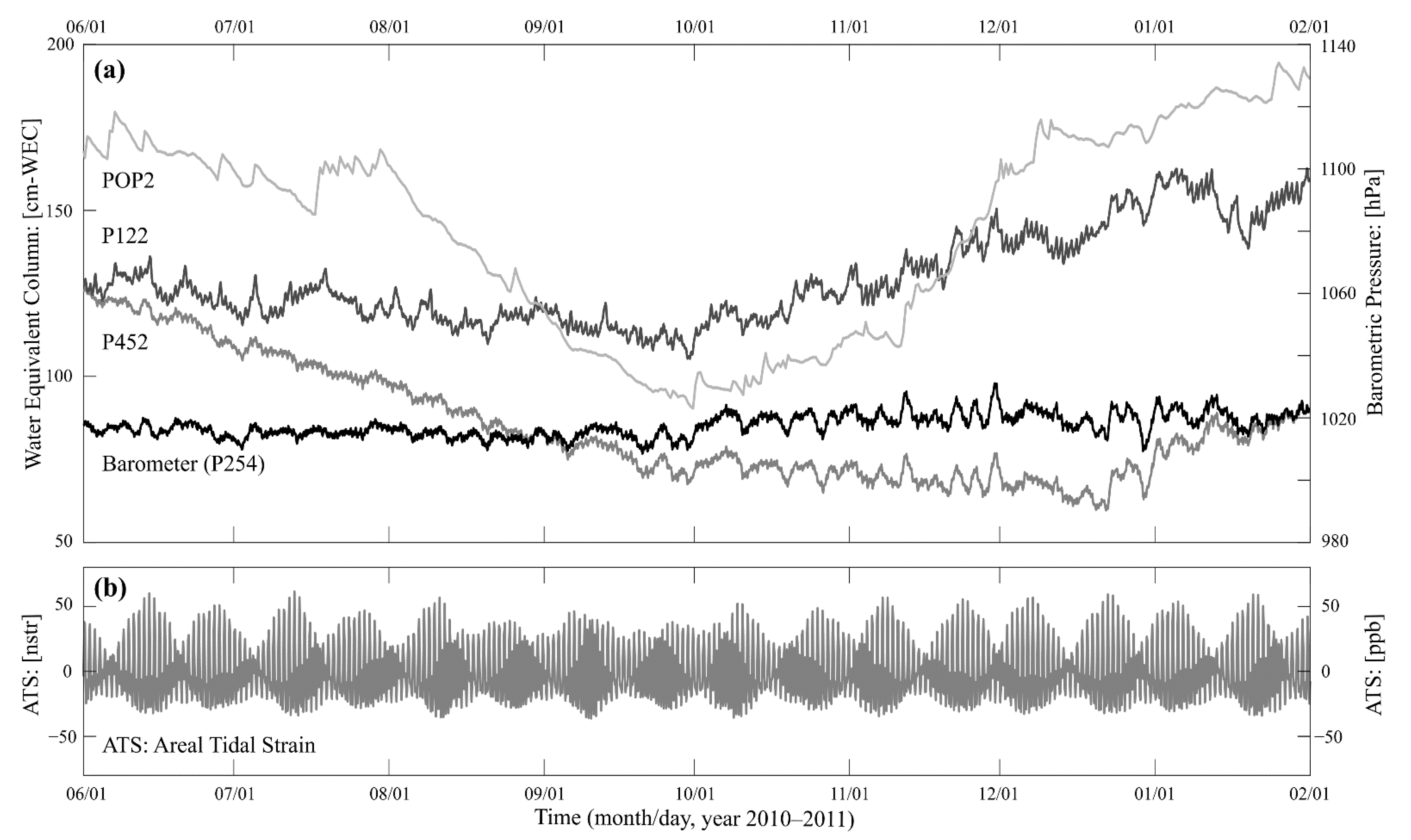
3.2. Data
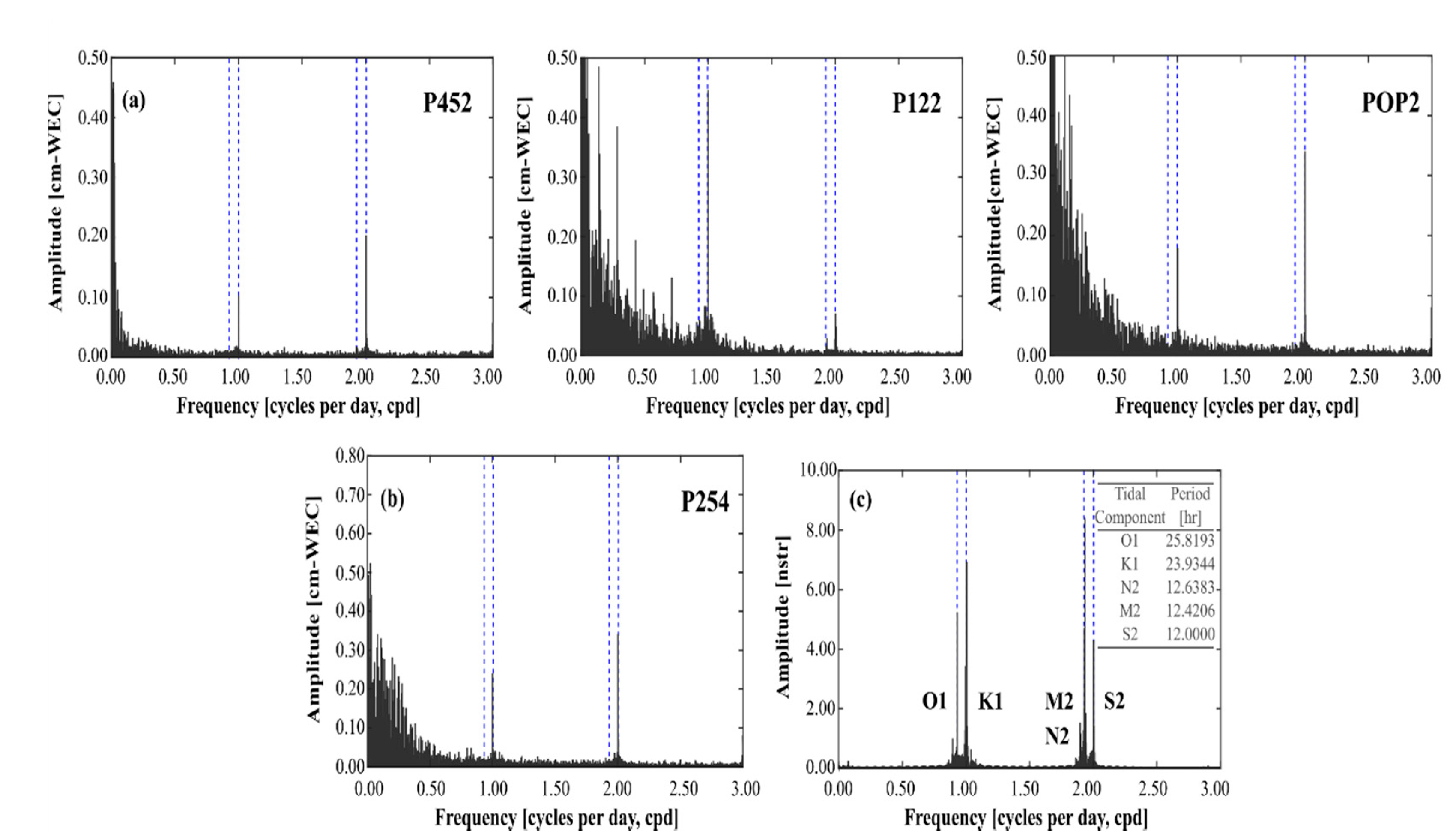
3.3. Data Processing
4. Results and Discussion
5. Conclusions
Author Contributions
Funding
Data Availability Statement
Acknowledgments
Conflicts of Interest
References
- Andrade-Borbolla, M. Actualización hidrogeológica del Valle de Guadalupe, Municipio de Ensenada, Baja California; Grupo Agroindustrial Valle de Guadalupe: Ensenada, Mexico, 1997; p. 66. (In Spanish) [Google Scholar]
- Campos-Gaytán, J.R. Simulación Del Flujo de Agua Subterránea en El Acuífero Del Valle de Guadalupe. Ph.D. Thesis, Centro de Investigación Científica y de Educación Superior de Ensenada, Ensenada, Mexico, 2008; 240p. (In Spanish). Available online: https://biblioteca.cicese.mx/catalogo/tesis/ficha.php?id=17841 (accessed on 14 May 2021).
- Gonzalez-Ramirez, J.; González, R.V. Modeling of the water table level response due to extraordinary precipitation events: The case of the guadalupe valley aquifer. Int. J. Geosci. 2013, 4, 950–958. [Google Scholar] [CrossRef] [Green Version]
- CNA; Comisión Nacional del Agua. Actualización de la Disponibilidad Media Anual de Agua en El Acuífero Guadalupe (0207); Comisión Nacional del Agua: Mexico, Mexico, 2018; 28p, (In Spanish). Available online: https://sigagis.conagua.gob.mx/gas1/Edos_Acuiferos_18/BajaCalifornia/DR_0207.pdf (accessed on 14 May 2021).
- Ramírez-Hernández, J.; Carreón, C.D.; Campbell, R.H.; Palacios, B.R.; Leyva, C.O.; Ruíz, M.L.; Vázquez, G.R.; Rousseau, F.P.; Campos, G.R.; Mendoza, E.L.; et al. Informe Final. Plan de Manejo Integrado de las Aguas Subterráneas en el Acuífero de Guadalupe, Estado de Baja California. Tomo I. Reporte Interno. Elaborado por la; Convenio: SGT-OCPBC-BC-07-GAS-001; Universidad Autónoma de Baja California para la Comisión Nacional del Agua, Organismo de Cuenca Península de Baja California, Dirección Técnica: Ensenada, Mexico, 2007. (In Spanish) [Google Scholar]
- Vázquez-González, R.; Romo-Jones, J.M.; Kretzschmar, T. Estudio Técnico Para El Manejo Integral Del Agua en El Valle de Guadalupe; División de Ciencias de la Tierra, Centro de Investigación Científica y de Educación Superior de Ensenada: Baja California, Mexico, 2007; p. 53. (In Spanish) [Google Scholar]
- Fuentes-Arreazola, M.A. Estimación de Parámetros Geohidrológicos, Poroelásticos Y Geomecánicos Con Base en El análisis de Las Variaciones Del Nivel Del Agua Subterránea en Pozos de Monitoreo en El Valle de Mexicali. Ph.D. Thesis, Centro de Investigación Científica y de Educación Superior de Ensenada, Baja California, Mexico, 2018; p. 127. (In Spanish). Available online: https://biblioteca.cicese.mx/catalogo/tesis/ficha.php?id=25077 (accessed on 14 May 2021).
- Jacob, C.E. Flow of groundwater. In Engineering Hydraulic; Rouse, H., Ed.; John Wiley & Son, Inc.: New York, NY, USA, 1950; pp. 321–386. [Google Scholar]
- Cooper, H.H.; Bredehoeft, J.D.; Papadopulos, I.S.; Bennett, R.R. The response of well-aquifer systems to seismic waves. J. Geophys. Res. Space Phys. 1965, 70, 3915–3926. [Google Scholar] [CrossRef]
- Bredehoeft, J.D. Response of well-aquifer systems to Earth tides. J. Geophys. Res. Space Phys. 1967, 72, 3075–3087. [Google Scholar] [CrossRef]
- Van Der Kamp, G.; Gale, J.E. Theory of earth tide and barometric effects in porous formations with compressible grains. Water Resour. Res. 1983, 19, 538–544. [Google Scholar] [CrossRef]
- Roeloffs, E.A. Hydrologic precursors to earthquakes: A review. Pure Appl. Geophys. 1988, 126, 177–209. [Google Scholar] [CrossRef]
- Rojstaczer, S.; Agnew, D. The influence of formation material properties on the response of water levels in wells to Earth tides and atmospheric loading. J. Geophys. Res. Space Phys. 1989, 94, 12403–12411. [Google Scholar] [CrossRef]
- Merritt, M.L. Estimating Hydraulic Properties of the Floridan Aquifer System by Analysis of Earth-Tide, Ocean-Tide, And Barometric Effects, Collier and Hendry Counties, Florida; US Geological Survey: Reston, VA, USA, 2004; p. 80.
- Fuentes-Arreazola, M.A.; Vázquez-González, R. Estimation of some geohydrological properties in a set of monitoring wells in Mexicali Valley, B.C., México. Revista Ingeniería del Agua 2016, 20, 87. [Google Scholar] [CrossRef] [Green Version]
- Fuentes-Arreazola, M.A.; Ramírez-Hernández, J.; Vázquez-González, R. Hydrogeological properties estimation from groundwater level natural fluctuations analysis as a low-cost tool for the Mexicali Valley aquifer. Water 2018, 10, 586. [Google Scholar] [CrossRef] [Green Version]
- Cutillo, P.A.; Bredehoeft, J.D. Estimating aquifer properties from the water level response to earth tides. Ground Water 2010, 49, 600–610. [Google Scholar] [CrossRef] [PubMed]
- Rasmussen, T.; Crawford, L.A. Identifying and removing barometric pressure effects in confined and unconfined aquifers. Ground Water 1997, 35, 502–511. [Google Scholar] [CrossRef]
- Weeks, P.E. Barometric fluctuations in wells tapping deep unconfined aquifers. Water Resour. Res. 1979, 15, 1167–1176. [Google Scholar] [CrossRef]
- Galloway, D.; Rojstaczer, S. Analysis of the frequency response of water levels in wells to earth tides and atmospheric loading. In Proceedings of the Fourth Canadian/American Conference in Hydrogeology; Canada National Ground Water Association: Banff, AB, Canada, 1988; pp. 100–113. [Google Scholar]
- Rahi, K.A.; Halihan, T. Identifying aquifer type in fractured rock aquifers using harmonic analysis. Ground Water 2013, 51, 76–82. [Google Scholar] [CrossRef]
- Clark, W.E. Computing the barometric efficiency of a well. J. Hydraul. Div. 1967, 93, 93–98. [Google Scholar] [CrossRef]
- Toll, N.J.; Rasmussen, T. Removal of barometric pressure effects and earth tides from observed water levels. Ground Water 2007, 45, 101–105. [Google Scholar] [CrossRef] [PubMed]
- Rahi, K.A. Estimating the Hydraulic Parameters of the Arbuckle-Simpson Aquifer by Analysis of Naturally-Induced Stresses. Ph.D. Dissertation, Oklahoma State University, Oklahoma, OK, USA, 2010; p. 168. Available online: https://core.ac.uk/download/pdf/215232243.pdf (accessed on 14 May 2021).
- Rojstaczer, S. Intermediate period response of water levels in wells to crustal strain: Sensitivity and noise level. J. Geophys. Res. Space Phys. 1988, 93, 13619–13634. [Google Scholar] [CrossRef] [Green Version]
- Rojstaczer, S. Determination of fluid flow properties from the response of water levels in wells to atmospheric loading. Water Resour. Res. 1988, 24, 1927–1938. [Google Scholar] [CrossRef] [Green Version]
- Lai, G.; Ge, H.; Wang, W. Transfer functions of the well-aquifer systems response to atmospheric loading and Earth tide from low to high-frequency band. J. Geophys. Res. Solid Earth 2013, 118, 1904–1924. [Google Scholar] [CrossRef]
- Harrison, J.C. New Computer Programs for the Calculation of Earth Tides; Cooperative Institute for Research in Environmental Sciences: Colorado, CO, USA, 1971; p. 30. [Google Scholar]
- Berger, J.; Beaumont, C. An analysis of tidal strain observation from the United States of America II: The inhomoge-neous tide. Bull. Seismol. Soc. Am. 1976, 66, 1821–1846. [Google Scholar]
- Harrison, J.C. Cavity and topographic effects in tilt and strain measurement. J. Geophys. Res. Space Phys. 1976, 81, 319–328. [Google Scholar] [CrossRef]
- Agnew, D.C. Earth tides. In Treatise on Geophysics and Geodesy; Herring, T.A., Ed.; Elsevier: New York, NY, USA, 2007; pp. 163–195. [Google Scholar]
- Doodson, A.T.; Warburg, H.D. Admiralty Manual of Tides; Her Majesty´s Stationary Office: London, UK, 1941; p. 270. [Google Scholar]
- Jacob, C.E. On the flow of water in an elastic artesian aquifer. Trans. Am. Geophys. Union 1940, 21, 574–586. [Google Scholar] [CrossRef]
- Hsieh, P.A.; Bredehoeft, J.D.; Farr, J.M. Determination of aquifer transmissivity from Earth tide analysis. Water Resour. Res. 1987, 23, 1824–1832. [Google Scholar] [CrossRef]
- INEGI. Datos de geología del Instituto Nacional de Estadística y Geografía. 2018. Available online: http://gaia.inegi.org.mx/mdm6/ (accessed on 14 May 2021).
- SGM. Sistema GEOINFOMEX del Servicio Geológico Mexicano. 2018. Available online: https://www.sgm.gob.mx/GeoInfoMexGobMx (accessed on 14 May 2021).
- García, E. Modificaciones Al Sistema de Clasificación Climática de Köpen Para Adaptarlo a Las Condiciones de la República Mexicana; Instituto de Geografía, Universidad Nacional Autónoma de México: Ciudad Universitaria, Mexico, 1981; p. 97, (In Spanish). Available online: http://www.publicaciones.igg.unam.mx/index.php/ig/catalog/view/83/82/251-1 (accessed on 14 May 2021).
- Molina-Navarro, E.; Hallack-Alegría, M.; Martínez-Pérez, S.; Ramírez-Hernández, J.; Moctezuma, A.M.; Sastre-Merlín, A. Hydrological modeling and climate change impacts in an agricultural semiarid region. Case study: Guadalupe River basin, Mexico. Agric. Water Manag. 2016, 175, 29–42. [Google Scholar] [CrossRef]
- Hallack-Alegría, M.; Ramírez-Hernández, J.; Watkins, D.W. ENSO-conditioned rainfall drought frequency analysis in northwest Baja California, Mexico. Int. J. Clim. 2011, 32, 831–842. [Google Scholar] [CrossRef]
- Del Toro-Guerrero, F.J.; Kretzschmar, T.; Hinojosa-Corona, A. Estimación del balance hídrico en una Cuenca semiárida, El Mogor, Baja California, México. Technol. Cienc. Agua 2014, 5, 69–81. [Google Scholar]
- Campos-Gaytán, J.R.; Kretzschmar, T. Numerical understanding of regional scale water table behavior in the Guada-lupe Valley aquifer, Baja California, Mexico. Hydrol. Earth Syst. Sci. Discuss. 2006, 3, 707–730. [Google Scholar] [CrossRef] [Green Version]
- Odong, J. Evaluation of empirical formulae for determination of hydraulic conductivity based on grain-size analysis. J. Am. Sci. 2007, 3, 54–60. [Google Scholar]
- Montecelos-Zamora, Y. Modelación Del Efecto de la Variación Climática en El Balance Hídrico en Dos Cuencas (México Y Cuba) Bajo Un Escenario de Cambio Climático. Ph.D. Thesis, Centro de Investigación Científica y de Educación Superior de Ensenada: Baja California, Mexico, 2018; p. 100. (In Spanish). Available online: https://biblioteca.cicese.mx/catalogo/tesis/ficha.php?id=25188 (accessed on 14 May 2021).
- Berger, J.; Farrell, W.; Harrison, J.C.; Levine, J.; Agnew, D.C. ERTID 1: A Program for Calculation of Solid Earth Tides; Technical Report; Scripps Institution of Oceanography: La Jolla, CA, USA, 1987; p. 20. [Google Scholar]
- Agnew, D.C. SPOTL: Some Programs for Ocean-Tides Loading; Technical Report; Scripps Institution of Oceanography: La Jolla, CA, USA, 2012; p. 30. Available online: https://igppweb.ucsd.edu/~agnew/Spotl/spotlmain.html (accessed on 14 May 2021).
- Pawlowicz, R.; Beardsley, B.; Lentz, S. Classical tidal harmonic analysis including error estimates in MATLAB using T_TIDE. Comput. Geosci. 2002, 28, 929–937. [Google Scholar] [CrossRef]
- Gercek, H. Poisson’s ratio values for rocks. Int. J. Rock Mech. Min. Sci. 2007, 44, 1–13. [Google Scholar] [CrossRef]
- Melchior, P. Earth tides. In Research in Geophysics; Odishaw, H., Ed.; Massachusetts Institute of Technology Press: Cambridge, MA, USA, 1964; pp. 183–193. [Google Scholar]
- Rojstaczer, S.; Riley, F.S. Response of the water level in a well to Earth tides and atmospheric loading under unconfined conditions. Water Resour. Res. 1990, 26, 1803–1817. [Google Scholar] [CrossRef] [Green Version]
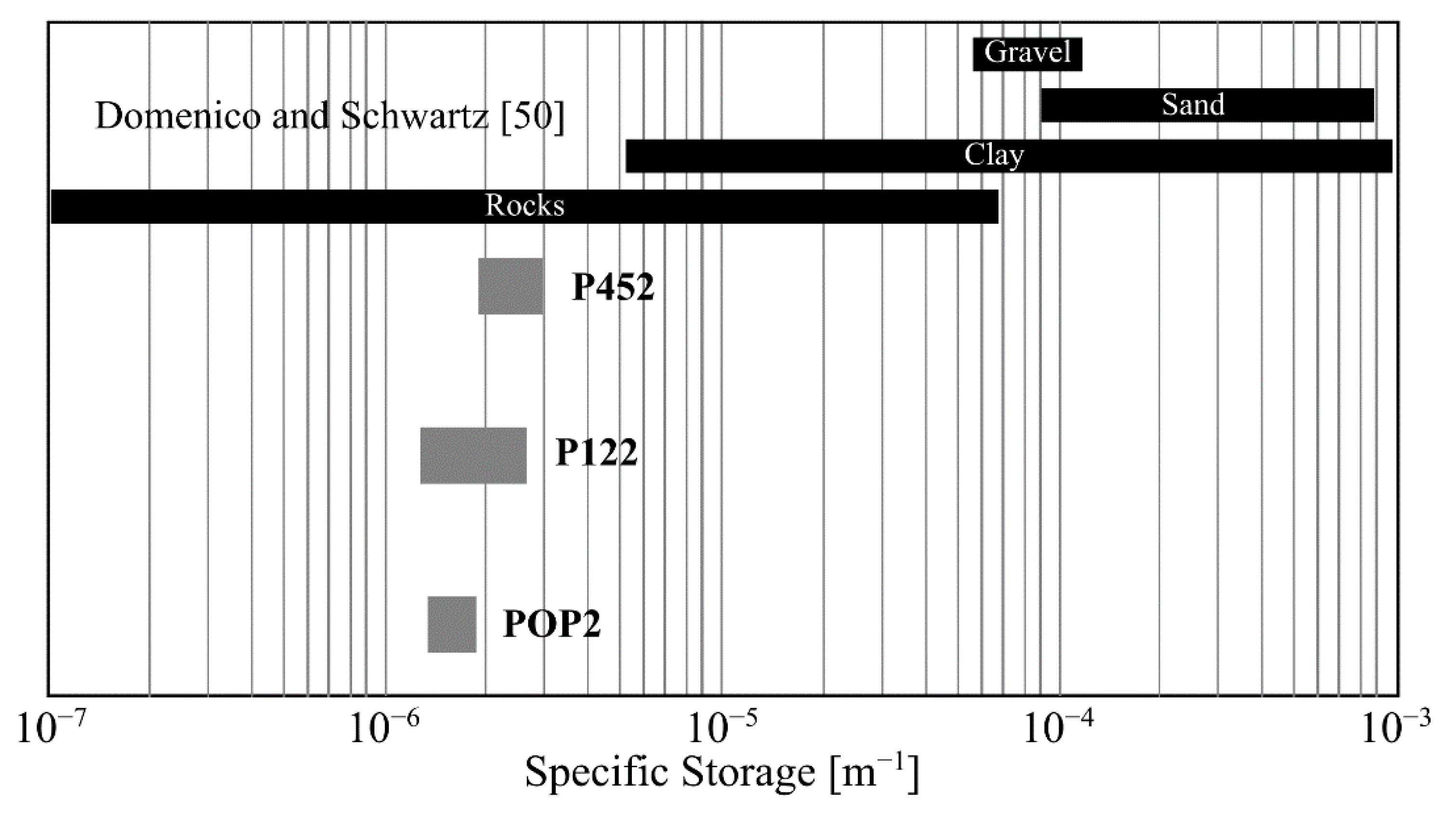
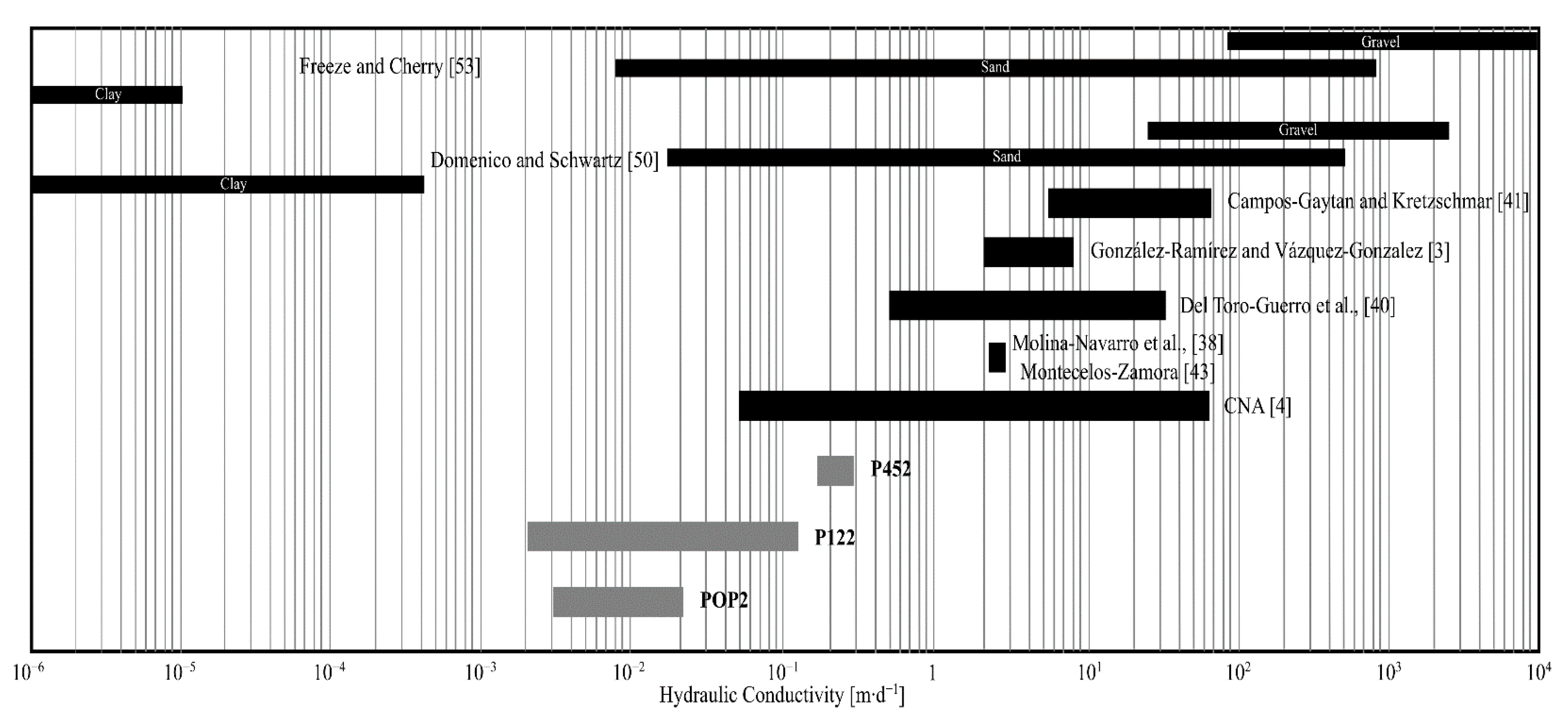
- Domenico, P.A.; Schwartz, F.W. Groundwater movement, hydraulic conductivity and permeability of geological material. In Physical and Chemical Hydrogeology, 2nd ed.; John Wiley & Sons, Inc.: New York, NY, USA, 1997; pp. 33–54. [Google Scholar]
- Hernández-Rosas, M.; Mejía-Vázquez, R. Relación de las Aguas Superficiales y Subterráneas del Acuífero BC-07; Gerencia Regional de la Península de Baja California, Subgerencia Regional Técnica, Technical Report; Comisión Nacional del Agua: Valle de Guadalupe, Mexico, 2003; p. 13. (In Spanish) [Google Scholar]
- Monge-Cerda, F.E. Detección Del Nivel Freático Con Métodos Geoeléctricos: El Caso Del Valle de Guadalupe. Master’s Thesis, Centro de Investigación Científica y de Educación Superior de Ensenada, B.C. Baja California, Mexico, 2020; p. 97. (In Spanish). Available online: https://biblioteca.cicese.mx/catalogo/tesis/ficha.php?id=25639 (accessed on 14 May 2021).
- Freeze, R.A.; Cherry, J.A. Physical properties and principles. In Groundwater; Prentice-Hall, Inc.: Hoboken, NJ, USA, 1979; pp. 14–79. [Google Scholar]


| Well ID | Coordinates 1 | WHE | BD | WTE | RWC/RWS | B | |
|---|---|---|---|---|---|---|---|
| Longitude X (m) | Latitude Y (m) | (masl) | (m) | (msnmm) | (m) | (m) | |
| P452 | 532,619 | 3,546,036 | 301.80 | 40.00 | 299.40 | 0.33/0.10 | 37.60 |
| P122 | 536,402 | 3,550,067 | 323.07 | 40.00 | 307.50 | 0.30/0.10 | 24.43 |
| POP2 | 543,576 | 3,552,069 | 345.40 | 80.00 | 317.30 | 0.10/0.10 | 51.90 |
| Well ID | Name | Location | Depth | Lithology |
|---|---|---|---|---|
| (m) | Material (Interval) | |||
| P01 | Porvenir-1 | ~1000 m NE-direction from P452 | 28.57 | 1. Sand (0 to 8 m) |
| 2. Sand and gravel (8 to 14 m) | ||||
| 3. Sandy clay (14 to 16 m) | ||||
| 4. Sand, gravel, clay (16 to 24 m) | ||||
| 5. Granite (24 to 30 m) | ||||
| P02 | Porvenir-2 | ~650 m W-direction from P122 | 41.70 | 1. Sandy clay (0 to 2 m) |
| 2. Sand (2 to 6 m) | ||||
| 3. Altered granite (6 to 16) | ||||
| 4. Fractured granite (16 to 40 m) | ||||
| PG2 | Guadalupe-2 | ~400 m NE-direction from POP2 | 83.90 | 1. Alternating layers of sand and gravel. The igneous basement was not drilled. |
| Well ID | Adhk∙(10−1) | Φdhk | ATk | ΦTk | ηk | ASk∙(10−2) | BE |
|---|---|---|---|---|---|---|---|
| (mm) | (°) | (nstr) | (°) | (°) | (mm∙nstr−1) | (%) | |
| O1/M2 | O1/M2 | O1/M2 | O1/M2 | O1/M2 | O1/M2 | ||
| P-452 | 1.61/4.24 | −68/−83 | 10.67/19.89 | −81/−44 | 13/−39 | 1.51/2.13 | 41.46 |
| P-122 | 10.57/5.98 | 55/−35 | 10.67/19.88 | 89/48 | −34/−83 | 9.90/3.01 | 48.32 |
| POP-2 | 1.21/2.66 | 66/78 | 10.68/19.87 | −78/16 | −12/62 | 1.13/1.34 | 79.79 |
| Well ID | SS (10−6) | φ | SC (10−5) | T (10−6) | K (10−2) |
|---|---|---|---|---|---|
| (m−1) | (%) | (m2∙s−1) | (m∙d−1) | ||
| O1/M2 | O1/M2 | O1/M2 | O1/M2 | O1/M2 | |
| P-452 | 2.78/1.93 | 26.88/18.60 | 10.45/7.26 | 129.46/74.28 | 29.75/17.07 |
| P-122 | 1.27/2.53 | 14.22/28.46 | 3.10/6.18 | 32.05/0.66 | 11.33/0.23 |
| POP-2 | 1.83/1.52 | 33.95/28.27 | 9.49/7.88 | 12.38/1.99 | 2.06/0.33 |
Publisher’s Note: MDPI stays neutral with regard to jurisdictional claims in published maps and institutional affiliations. |
© 2021 by the authors. Licensee MDPI, Basel, Switzerland. This article is an open access article distributed under the terms and conditions of the Creative Commons Attribution (CC BY) license (https://creativecommons.org/licenses/by/4.0/).
Share and Cite
Fuentes-Arreazola, M.A.; Ramírez-Hernández, J.; Vázquez-González, R.; Núñez, D.; Díaz-Fernández, A.; González-Ramírez, J. Aquifer Parameters Estimation from Natural Groundwater Level Fluctuations at the Mexican Wine-Producing Region Guadalupe Valley, BC. Water 2021, 13, 2437. https://doi.org/10.3390/w13172437
Fuentes-Arreazola MA, Ramírez-Hernández J, Vázquez-González R, Núñez D, Díaz-Fernández A, González-Ramírez J. Aquifer Parameters Estimation from Natural Groundwater Level Fluctuations at the Mexican Wine-Producing Region Guadalupe Valley, BC. Water. 2021; 13(17):2437. https://doi.org/10.3390/w13172437
Chicago/Turabian StyleFuentes-Arreazola, Mario A., Jorge Ramírez-Hernández, Rogelio Vázquez-González, Diana Núñez, Alejandro Díaz-Fernández, and Javier González-Ramírez. 2021. "Aquifer Parameters Estimation from Natural Groundwater Level Fluctuations at the Mexican Wine-Producing Region Guadalupe Valley, BC" Water 13, no. 17: 2437. https://doi.org/10.3390/w13172437