
Predicting Inflow Rate of the Soyang River Dam Using Deep Learning Techniques


1
Department of Applied Data Science, Sungkyunkwan University, Suwon 16419, Korea
2
School of Convergence, Sungkyunkwan University, Seoul 03063, Korea
*
Author to whom correspondence should be addressed.
Water 2021, 13(17), 2447; https://doi.org/10.3390/w13172447
Submission received: 27 July 2021
/
Revised: 26 August 2021
/
Accepted: 3 September 2021
/
Published: 6 September 2021
(This article belongs to the Section Hydrology)
Abstract
:The Soyang Dam, the largest multipurpose dam in Korea, faces water resource management challenges due to global warming. Global warming increases the duration and frequency of days with high temperatures and extreme precipitation events. Therefore, it is crucial to accurately predict the inflow rate for water resource management because it helps plan for flood, drought, and power generation in the Seoul metropolitan area. However, the lack of hydrological data for the Soyang River Dam causes a physical-based model to predict the inflow rate inaccurately. This study uses nearly 15 years of meteorological, dam, and weather warning data to overcome the lack of hydrological data and predict the inflow rate over two days. In addition, a sequence-to-sequence (Seq2Seq) mechanism combined with a bidirectional long short-term memory (LSTM) is developed to predict the inflow rate. The proposed model exhibits state-of-the-art prediction accuracy with root mean square error (RMSE) of 44.17 m3/s and 58.59 m3/s, mean absolute error (MAE) of 14.94 m3/s and 17.11 m3/s, and Nash–Sutcliffe efficiency (NSE) of 0.96 and 0.94, for forecasting first and second day, respectively.
1. Introduction
Due to its high population density, South Korea has only one-sixth of the world’s average water available per capita and suffers from deterioration of water resource quality, floods, and droughts due to significant variance in yearly regional and seasonal precipitation [1]. In particular, islands and mountainous areas suffer from annual water shortages that require the use of emergency water supplies with restrictions on water usage. These shortages are due to low water inflow, specifically on tributary streams with delayed investment in infrastructure, causing an increase in damage of water-related natural disasters [1,2]. To overcome these issues, Korea has constructed multipurpose dams to manage water resources. However, climate change significantly increases the probability of water-related disasters (e.g., floods and droughts) and adds to the uncertainty of water resource management [2]. Consequently, climate change alters dam inflow patterns, adding difficulties to water supply and water resource utilization plans [3]. According to Jung et al. [4], researchers previously used conceptual and physical hydrologic models to predict the water level or inflow rate of the dam; however, these models must include meteorological and geological data, and prediction accuracy varies based on the number of parameters. In addition, conceptual and physical hydrologic models require constant verification and adjustment of each input parameter, causing an increase in simulation time and reducing the overall time to prepare for a natural disaster. Researchers have used various models, such as the Hydrological Simulation Program—Fortran [5], the watershed-scale Long-Term Hydrologic Impact Assessment Model [6], and the Soil and Water Assessment Tool (SWAT) [7], to predict the river discharge and dam inflow rate.
In the case of the Soyang River, some areas of the watershed are located in North Korea, resulting in insufficient hydrological data for prediction, and SWAT does not yield accurate inflow rate predictions. Furthermore, the Soyang Dam, a multipurpose dam that controls water supply and generates power for the Seoul metropolitan area, is located on the Soyang River. To overcome the lack of accurate hydrological data to predict the Soyang River Multipurpose Dam inflow, researchers have used data-driven models [8,9,10,11,12,13,14,15,16]. The proposed model not only can predict the inflow rate without detailed hydrological data but also outperforms the existing algorithms [8,9]. We believe that our model can be applied to other dams that do not have sufficient hydrological data for predicting the inflow rate.
Data-driven models are capable of repeatedly learning the complex nonlinear relationships between input and output data to produce highly predictive performance, regardless of the conceptual and physical characteristics. Researchers worldwide use data-driven models for various applications, such as decoding clinical biomarker space of COVID-19 [17], water quality prediction [18], and pipe-break rate prediction [19]. Researchers attempt to use data-driven models for various hydrological predictions, such as MARS [20,21,22,23,24], DENFIS [25], LSTM-ALO [26], and LSSVR-GSA [27]. MARS uses forward and backward step to add and remove piecewise linear functions to fit the model. However, there is performance degradation if data contain too many variables. To get the best result, MARS requires variable selection [20,21,22,23,24]. DENFIS requires prior assumptions about data and needs domain knowledge to set predefined parameters. Yuan et al. [26] claim that LSTM-ALO can find the optimal hyperparameter with an ant-lion optimizer. However, the model uses a variable to predict the runoff. Adnan et al. [27] claim that the gravitation search algorithm (GSA) will help to find the optimal value for the least square support vector regressor (LSSVR). LSSVR is a modified version of the support vector regressor (SVR) that reduces the complexity of the optimization program [24]. Even though LSSVR-GSA outperforms LSSVR, there was no mention that implementing GSA would reduce the overall training time.
In the case of inflow rate prediction, researchers used SVR [10,11,12], Comb_ML [9], multivariate adaptive regression splines (MARS) [28], random forest [9,10,11,12,13], and gradient boosting [9,11,14]. In addition, deep learning models, such as multilayer perceptron regressors (MLP) [9,10,13], recurrent neural networks (RNNs) [8], and LSTM [15,16], as the models for inflow rate predictions. These models have proven to be highly effective in predicting inflow rates, but they do not have the ability to capture input data’s long-term dependencies and summarize the data.
We propose an end-to-end model that consists of a Seq2Seq algorithm incorporated with bi-directional LSTM and a scaled exponential linear unit (SELU) activation function to predict the inflow rate over a period of two days. Then we evaluate and compare the model with other algorithms. The Seq2Seq model consists of an encoder and decoder. First, the encoder summarizes the information of the input sequence. Then the decoder uses the summarized information for prediction. We use LSTM for both an encoder and a decoder. LSTM consists of gating units to handle sequential data and learns long-term dependencies. In addition, we incorporated bidirectionality with LSTM to extract extra information about complex relationships between present and past data. Lastly, we change the activation function of LSTM from tanh to SELU with LeCun normal kernel initializers to stabilize the training process despite the presence of abnormally high and low inflow rates. We did not use any decomposition method because we believe bidirectional LSTM can extract information from flooding and drought events, and SELU activation function helps to stabilize the training process with the abnormal inflow rates. Our model proves that predicting the inflow rate is possible without using detailed hydrological data.
In this article, we construct some commonly used machine learning models to compare the prediction accuracy with the proposed model. Then, we evaluate the result of the proposed model by using a discrepancy ratio. We propose a deep learning algorithm that surpasses the prediction accuracy of the existing algorithms, such as RNN [8] and Comb-ML [9], in predicting the inflow rate of the Soyang Multipurpose Dam for a period of two days. We also compared the prediction accuracy of our model with those of the existing machine learning models.
The contributions of this study are as follows:
- We developed an end-to-end model capable of summarizing input data for inflow rate forecasting.
- Unlike previous research, we only used nearly 15 years of weather warning data, along with the meteorological and dam inflow rate data.
- Our Seq2Seq model used bidirectional LSTMs, SELU activation function, and LeCun normal kernel initializer to stabilize the training process and outperformed the baseline models in most accuracy criteria.
2. Materials and Methods
2.1. Study Area
This study predicts the inflow rate of the Soyang River Multipurpose Dam (Soyang Dam), the largest dam in Korea. The dam was built in 1973 and can hold up to 2.9 billion metric tons of water. The dam consists of five flood gates for various purposes. The Soyang Dam supplies water to Gangwon Province, Seoul metropolitan area, and Han River coast and prevents flooding of the downstream region of the Han River. It also generates and supplies electricity to the Seoul metropolitan area and Korea’s central region to cope with the surging demand for electricity [29]. However, dam management is increasingly complicated because of climate change and, as the annual precipitation increases, the inflow decreases owing to evaporation [9].
2.2. Data Description
Daily weather and daily dam data for this experiment were obtained from the Korea Water Resources Corporation [30] and the Korea Meteorological Administration [31], respectively. The data ranged from 4 July 2004 to 31 December 2019.
The dam data consist of many records, such as inflow rate, precipitation, discharge amount, and dam water level. For this study, we used only the daily inflow rate and daily precipitation records.
We collected weather data for Chuncheon City, where the dam is located. More than 100 daily meteorological records of Chuncheon City are available. However, we only collected the maximum and minimum temperatures, average wind speed, total solar radiation, and average humidity for each day. One average humidity, one total solar radiation, and two average wind speed data points were missing; we interpolated the missing data points using linear interpolation.
Weather warning data consist of city, regional, and province records of 30 warnings and watches, and each warning can be issued multiple times a day. In some cases, multiple warnings are in effect in a single day. The daily frequency of each warning was counted. The Soyang River Dam catchment spans Chuncheon City, Yeongseo, and the midwest regions of Gangwon Province. Therefore, we collected only warning types in effect in the catchment area, as shown in Table 1. Unlike the weather watch, the warning goes into effect when a disaster occurs, and major damage is expected [32]. As this experiment aims to predict the regular and extreme inflow rates accurately, we only collected the heavy rain warning data.
Figure 1 shows that rainfall and inflow increase and decrease simultaneously and that they are occasionally unusually high. The daily maximum and minimum temperatures, average wind speed, relative humidity, and total solar radiation exhibit no irregularities. Heavy rain warnings show similar patterns to the daily inflow rate and precipitation.
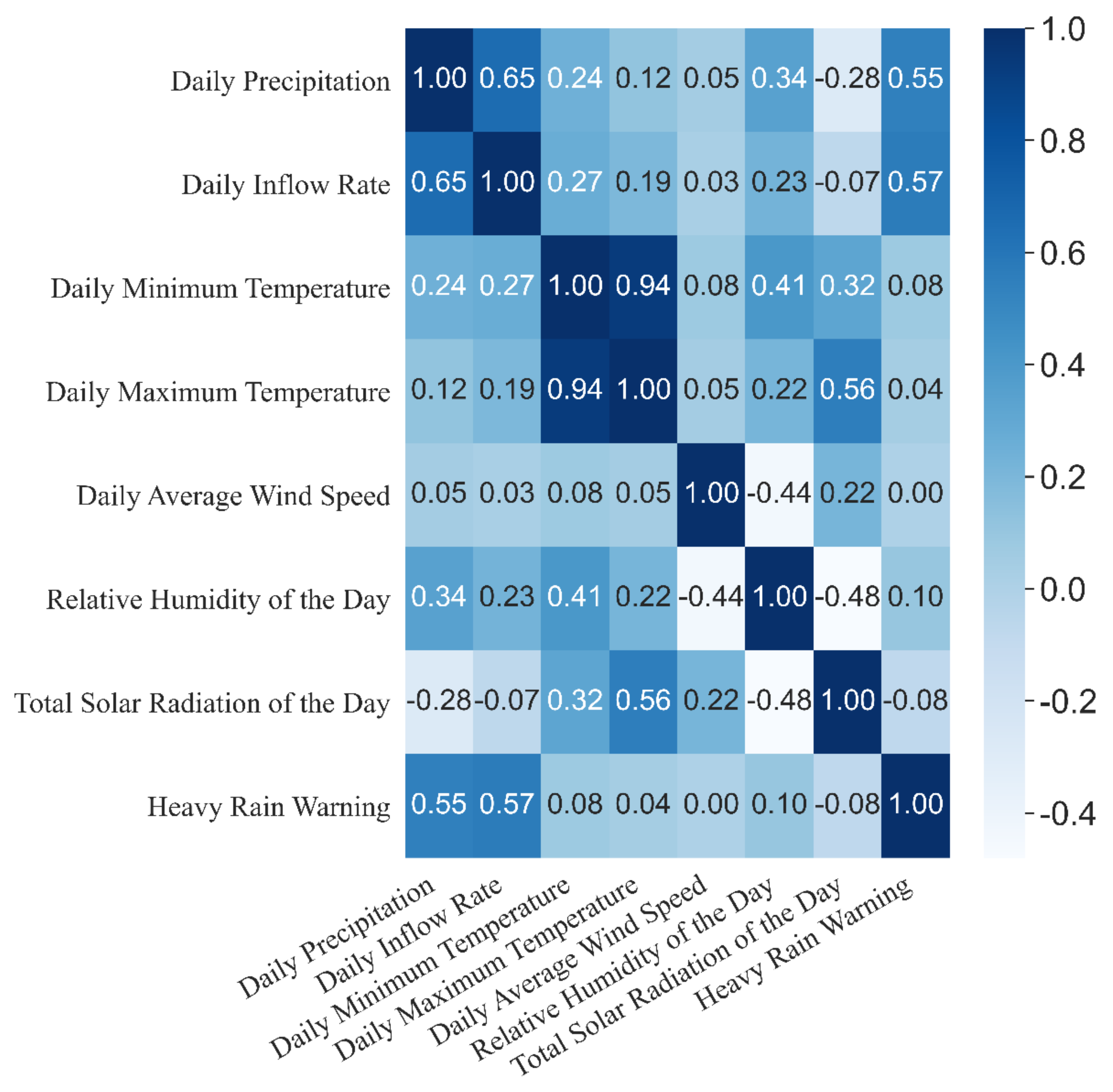
Figure 2 shows a heatmap of the correlation coefficients between the input variables. In addition to the daily minimum and maximum temperature correlation, there is a high correlation between the inflow rate, precipitation, and heavy rain warnings. Moreover, the heatmap suggests that the daily minimum and maximum temperatures, humidity, and total solar radiation have a high correlation.
Prior weather conditions have a significant effect on the amount of water in the soil [33]. Therefore, for this experiment, we included seven days of meteorological data as the input. In addition, previous research incorporates past daily inflow rates and forecasted rainfall for better inflow rate accuracy [8,9]. Therefore, we input the past seven days of meteorological data, inflow rate, and forecasted rainfall for the next two days, as listed in Table 1.
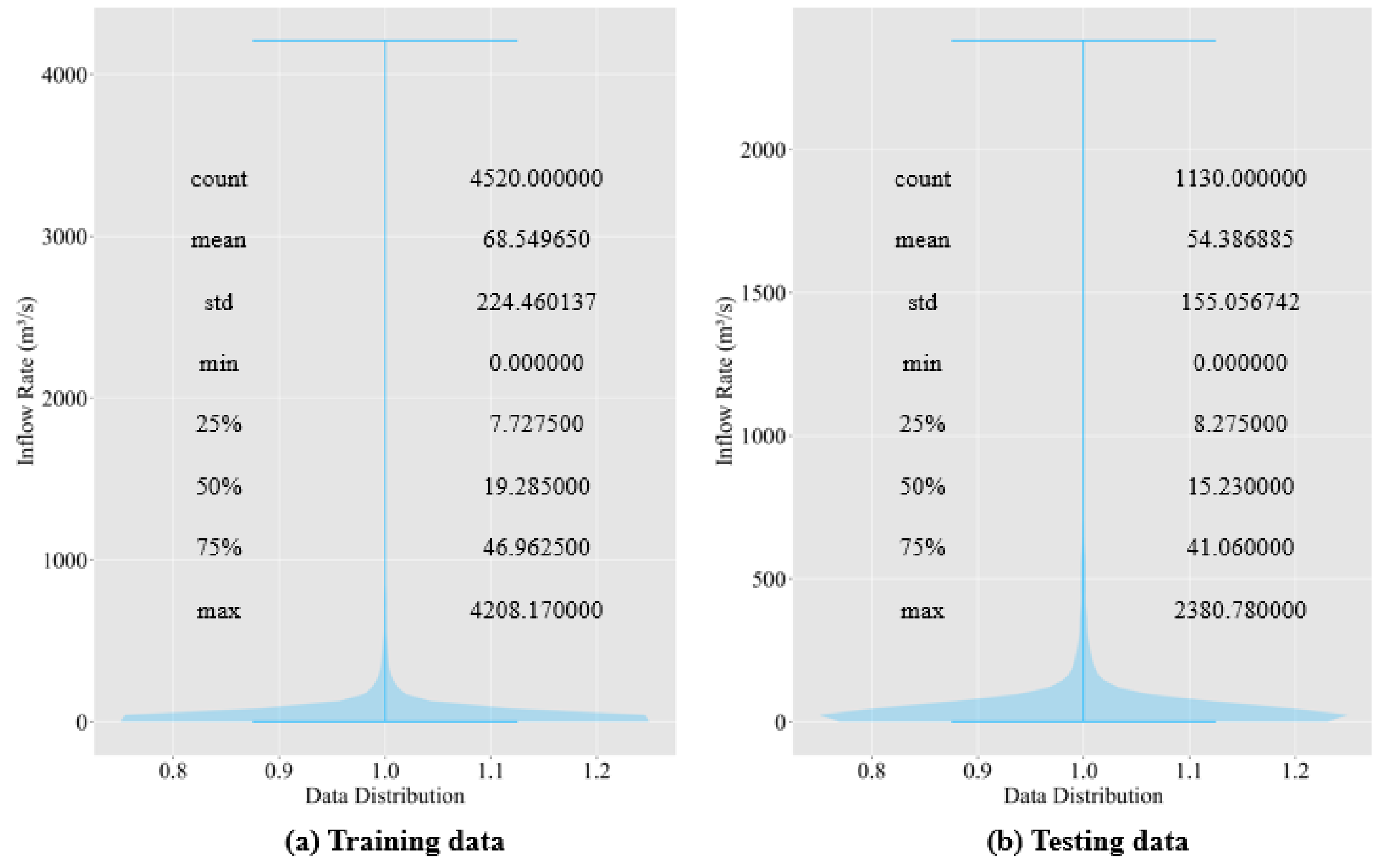
Figure 3 suggests that both the training and the testing data are left-skewed. The third interquartile for both training and testing data are less than 50 m3/s, and the maximum value is greater than 2300 m3/s. The noticeable difference between the third interquartile and the maximum value suggests that the Soyang River Dam deals with occasional heavy floods.
We standardized the input variables because each variable has different minimum and maximum values and distributions. Then, we reserved 20% of the data for testing and used the remaining for training.
We created an end-to-end model that can predict both normal and abnormally high inflow rate of the dam. We did not use any decomposition method because we want our model to extract information from flooding events and predict abnormally high inflow rates. Our model contains LSTM for both an encoder and a decoder. LSTM uses a gating function to capture essential information.
2.3. Background
We introduce the following two primary components that form the foundation of our model: a bidirectional LSTM and a sequence-to-sequence model.
2.3.1. Bidirectional LSTM
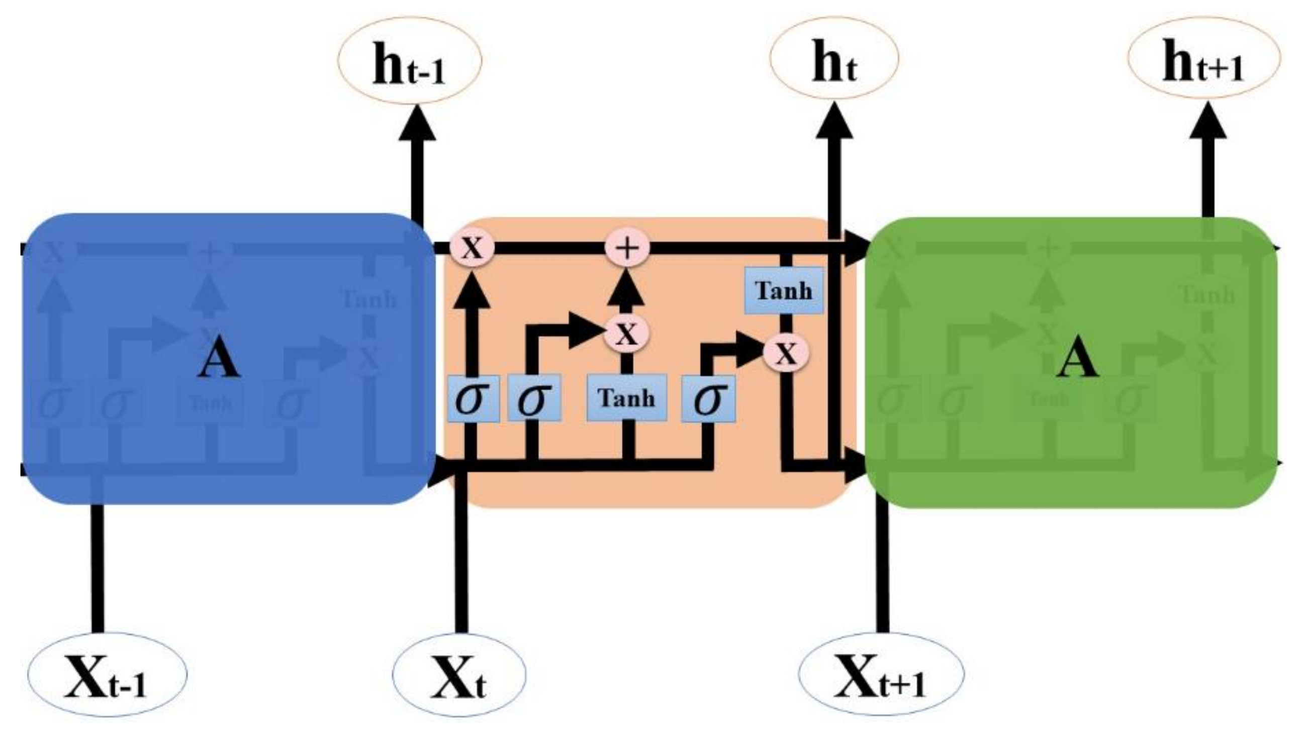
RNNs suffer from a vanishing gradient problem as the length of the sequence increases. To overcome this problem, LSTM uses gated functions to accept long sequences and decide which part of the input data to remember [34]. The structure of LSTM is shown in Figure 4. Equations (1)–(6) are equations for the LSTM [15], where Ot, ct, ht, and ft represent the input, output, cell state, hidden state, and forget state, respectively; t represents the time step, and xt is the input vector for LSTM. Wn, Wf, and Wi represent the weight of the output gate activation vector, forget gate activation vector, and input gate activation vector, respectively; σ is the activation function for the forgotten, hidden, and cell state gates. Nt uses the tanh activation function to update the weight of the input. Some researchers have used the LSTM to predict the inflow rate [15,16].
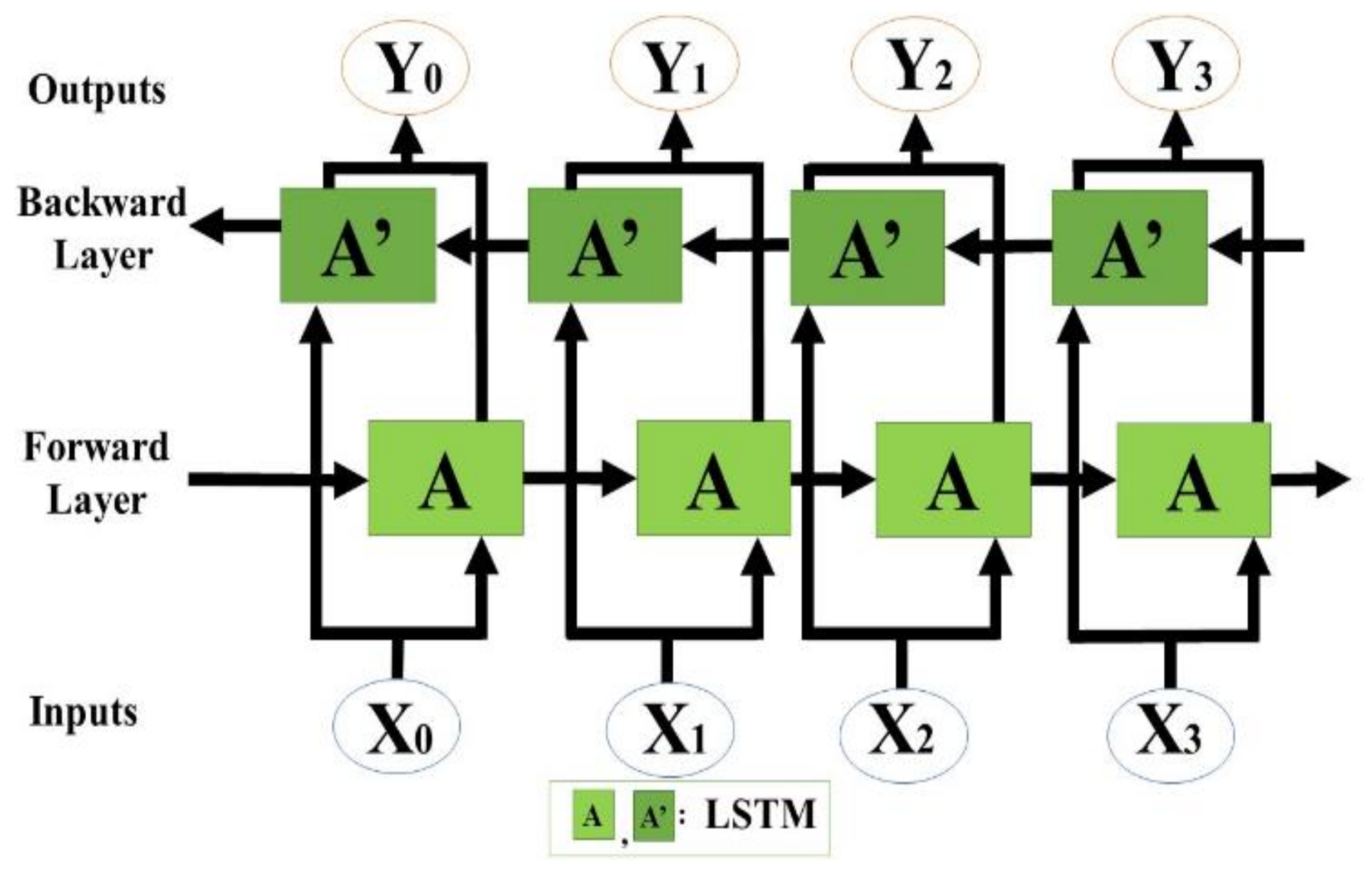
As shown in Figure 5, LSTM can be trained in both directions. Bidirectional LSTM combines a bidirectional RNN and LSTM [35]. A unidirectional LSTM processes data in the order of input and tends to predict based on recent patterns. In contrast, the bidirectional LSTM learns from both past to present and present to past data, providing a higher predictive performance than the unidirectional LSTM [36,37].
2.3.2. Seq2Seq Model
Suyskever et al. [38] introduced a Seq2Seq model consisting of an encoder and a decoder. The encoder compresses the input sequence data, and the decoder creates a sequence output based on the compressed data. The encoder uses an input sequence and outputs the hidden state vectors and resultant vectors to the decoder. The decoder then uses outputs from the encoder to train on the difference between the real and predicted values.
2.4. Experimental Setup
In this experiment, we compare the prediction accuracy of our model against the baseline models presented in Section 1: support vector regressor, random forest regressor, multilayer perceptron (MLP), Comb-ML, and RNN. Optimal hyperparameters are found for each model by performing a grid search. Then, we introduce our sequence-to-sequence model with bidirectional LSTMs. Finally, we show that our model is the most accurate model for predicting the inflow rate of the Soyang River Dam.
We use the mean absolute error (MAE), root mean square error (RMSE), and Nash–Sutcliffe Efficiency (NSE) as the metrics for the prediction accuracy. We decided to use RMSE, MAE, and NSE because they are the most popular statistical methods often used to compare observed values with the predicted values. In addition, Hong et al. [9] used RMSE, MAE, and NSE to evaluate the predictive performance of their model. Park et al. [8] used NSE and RMSE as performance metrics. Therefore, it is logical to use MAE, RMSE, and NSE to evaluate models. MAE measures how well our model predicts extreme events, such as floods and droughts. RMSE assesses the extent to which the predicted value is different from the mean of the real value. Finally, NSE measures the prediction accuracy of the hydrological model. The MAE and RMSE range from 0 to infinity, while the NSE ranges from negative infinity to 1. The model is predictive if NSE is approximately 1, while MAE and RMSE are approximately 0. MAE, RMSE, and NSE for the evaluation of the model accuracy can be calculated from Equations (7)–(9), where is the actual value at time j, is the predicted value at j, n is the number of days, and is the average of the observed values.
2.4.1. SVR (Baseline)
A SVR generates a hyperplane that does not exceed the maximum marginal error [39]. Equation (10) is used to find the hyperplane. and are constants from the Lagrange dual optimization, and b is a bias. K〈,x〉 is a kernel function: linear, polynomial, radial basis (RBF), or sigmoid function. Several studies have used different kernel functions to determine the optimal value to obtain the best prediction accuracy [10,11,12]. To find the optimal hyperparameters, we tested different values, as shown in Table 2. We tried different kernel functions and experimented with various degrees for the polynomial kernel. Gamma is the kernel coefficient for the polynomial and RBF kernels, and it had a significant impact on the predictive performance.
2.4.2. Random Forest Regressor (Baseline)
A random forest is an ensemble model of decision trees using a bagging method [40]. The model builds multiple decision trees and searches for the best features among a random subset of features [41]. As the regressor has only a few hyperparameters, it is easy to determine the optimal values [9,13]. As shown in Table 3, we experimented with different hyperparameter values to identify the best predictive model: n_estimators is the number of decision trees used in the experiment, and max_features is the number of features to be considered when searching for the best split. Finally, the criterion measures the quality of the split.
2.4.3. Gradient Boosting Regressor (Baseline)
Boosting is an ensemble technique that connects multiple weak learners to create multiple strong learners [42]. The gradient boosting regressor adds predictors sequentially to correct the errors. Liao et al. [14] created a model based on a gradient boosting regressor to predict the inflow rate more accurately than a support vector regressor and multilayer perceptron regressor model. We experimented with various hyperparameters to obtain the highest prediction accuracy, as shown in Table 4. Specifically, we experimented with different loss functions (loss), learning rates (learning_rate), numbers of trees (n_estimators), and criteria (criterion) for splitting nodes.
2.4.4. Multilayer Perceptron Regressor (Baseline)
In 1958, Rosenblatt first proposed an artificial neural network called perceptron [43]. In Equation (11), is the weight vector of the perceptron, and X is the input vector. In Equation (12), σ is the activation function of the resultant vector of the input vector multiplied by the weight vector, . Each layer of the neural network consists of one or more perceptrons. Each layer of the perceptron receives the output from the previous layer. The output from the final layer is compared with the result, and the weight is updated through backpropagation [44]. Previous research used the backpropagation algorithm to predict the inflow rate [9,12,13]. As shown in Table 5, we experimented with the number of perceptrons per hidden layer (hidden_layer_size), activation functions (activation), gradient descent algorithm (solver), number of training samples in one iteration (batch_size), learning rate (learning_rate), and a decision to shuffle the dataset (shuffle).
2.4.5. Comb-ML (Baseline)
The Comb-ML model combines MLP with either a random forest regressor or a gradient boosting model. Comb-ML first identifies the optimal hyperparameter for each model and then combines the models. According to Hong et al. [9], when the inflow rate exceeded 100 m3/s and the average precipitation was 16 mm, the MLP showed the highest prediction accuracy. In contrast, when the inflow rate was less than 100 m3/s, the ensemble models (random forest regressor and gradient boosting regressor) showed the highest prediction accuracy. Consequently, they created a model called RF_MLP, which combined MLP with a random forest regressor, and another model called GB_MLP, which combined MLP with a gradient boosting regressor called GB_MLP.
2.4.6. RNN (Baseline)
Unlike artificial networks with the feed-forward method, nodes in the RNN receive new data and data from the previous state. Park et al. [8] used the Soyang River Dam data and Chuncheon City meteorological data as inputs to the RNN. In addition, their RNN had three hidden layers, and each hidden layer had an extra node to account for the bias. We followed their method to create an RNN model. As shown in Table 6, we changed the learning rate and batch size to obtain the best prediction accuracy.
2.4.7. MARS (Baseline)
MARS is a nonparametric regression model. It finds a set of simple piecewise linear functions and combines them to predict until the residual error is too small. Then it removes the least effective term iteratively until it meets the stopping criteria [45]. MARS model is fitted using py-earth Python library [46].
2.4.8. Seq2Seq Model
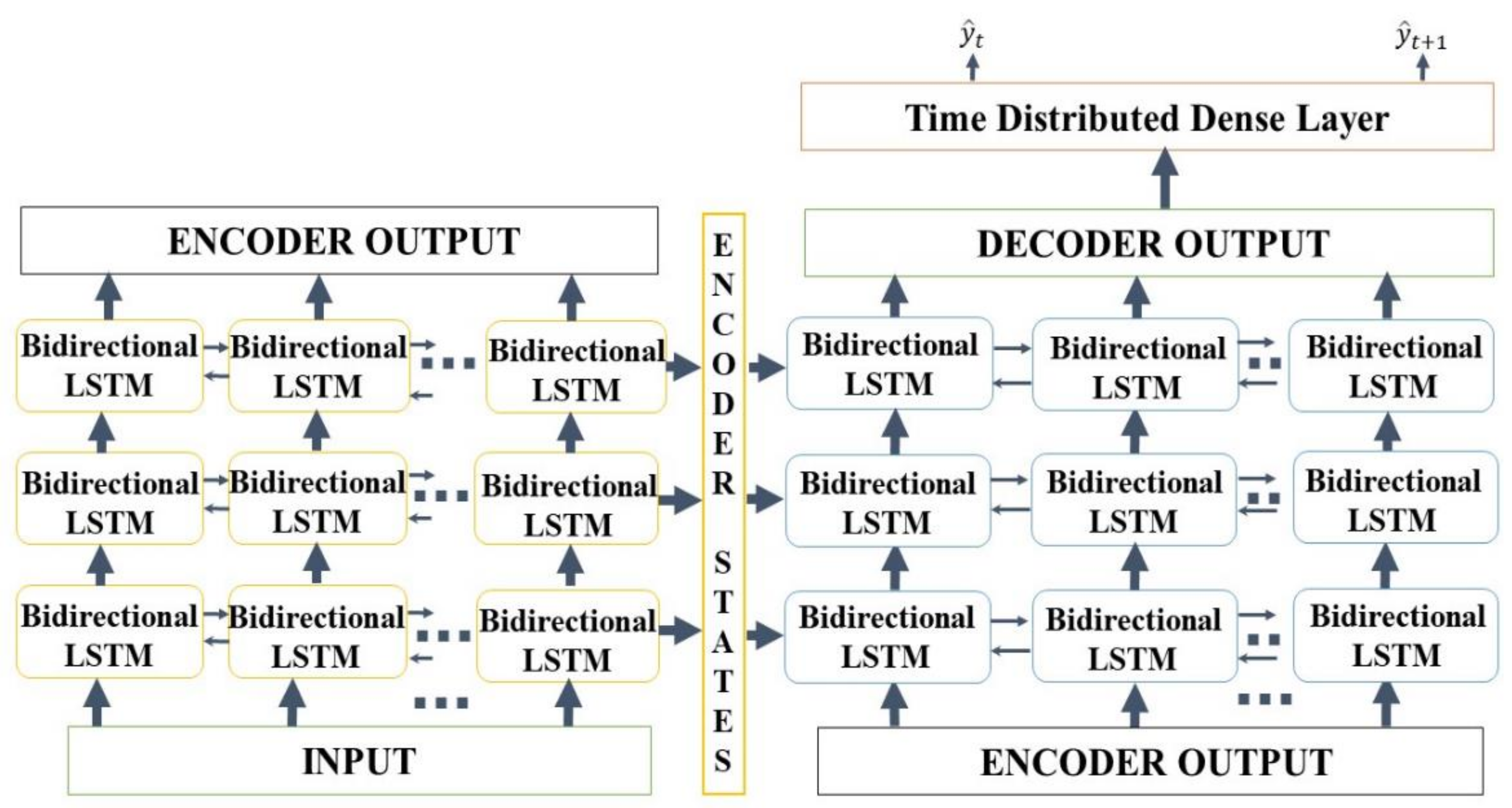
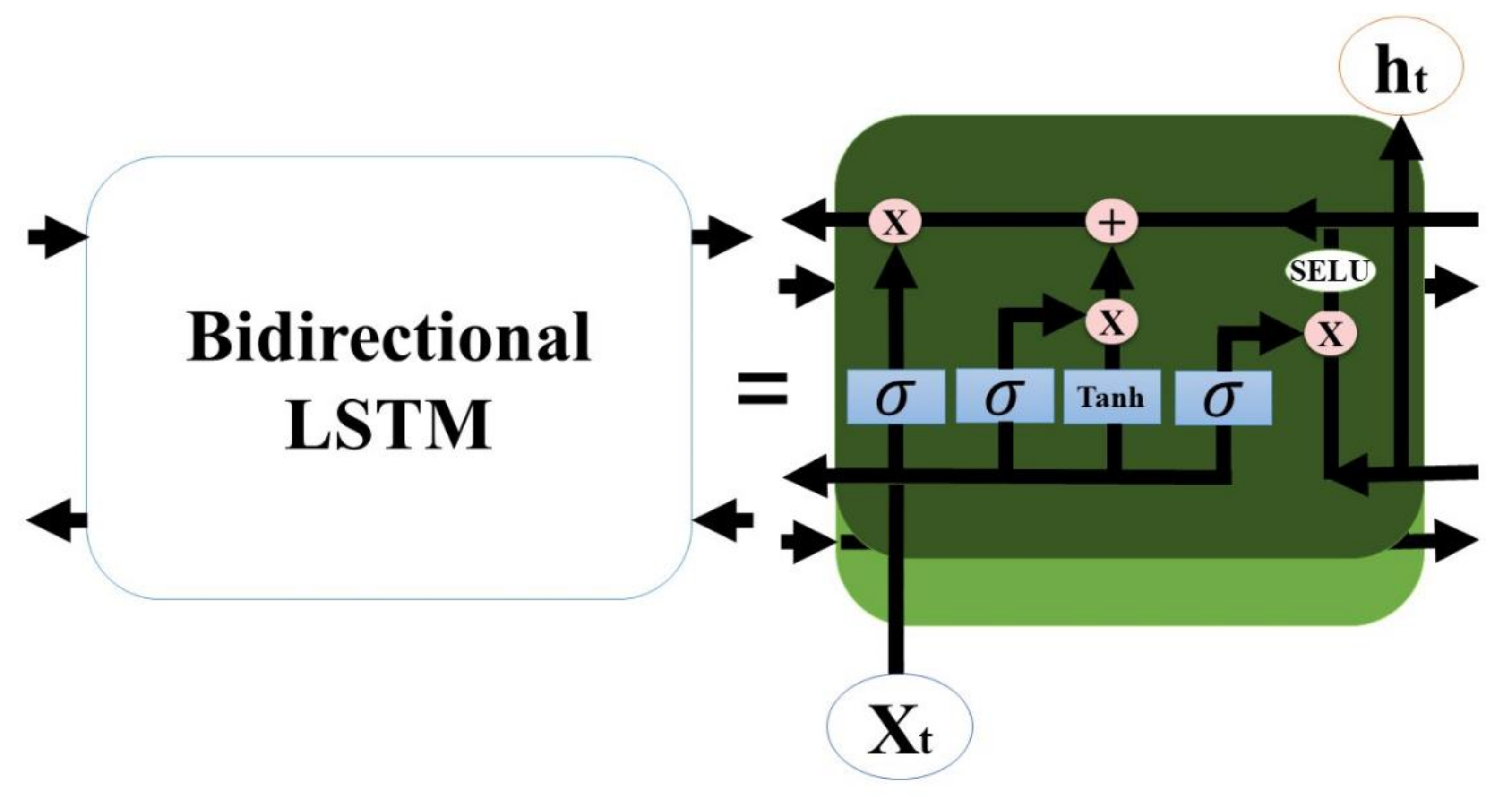
The Seq2Seq model has three layers of bidirectional LSTMs for an encoder and decoder, as shown in Figure 6. We utilize bidirectional LSTM (Figure 7) for an encoder and a decoder because it enables the model to train on the present to past and past to present information. For each bidirectional LSTM, we use the SELU activation function with the LeCun normal kernel initializer to stabilize the training in the cases of flood and drought seasons. Equation (13) represents the SELU activation equation. According to Klambauer et al. [47], α and λ are approximately 1.67 and 1.05, respectively. As shown in Table 7, we changed the learning rate, batch size, and number of output units for each bidirectional LSTM to obtain the best prediction accuracy. The learning rate and batch size, and the number of output units per bi-directional LSTM all affect how the model trains. We experiment with a different set of hyperparameters to achieve the best prediction accuracy, as shown in Table 7. The overall training procedure is described as shown in Algorithm 1 and Figure 8.
| Algorithm 1: Seq2Seq Training Procedure. | |
| Input: Weather data for the last seven days and forecasted rainfall | |
| Output: Predicted inflow rate for t and t + 1 | |
| 1: | For Epoch = Epoch + 1 to 3000 do |
| 2: | Initialize encoder kernel with LeCun Normal kernel initializer |
| 3: | Generate encoder output with SELU activation function |
| 3: | Obtain hidden and carry state data from encoder output |
| 4: | Initialize decoder with LeCun Normal kernel initializer |
| 5: | Generate decoder output with SELU activation function |
| 6: | Evaluate error between expected output and the model output with mean squared error |
3. Results
In this section, we share the prediction accuracy results of the baseline models and our proposed model. We then compare the results of the baseline and proposed models. Then, we list the outcomes of not using the SELU activation function and bidirectionality of LSTM in the Seq2Seq model. Finally, we share the results of not using heavy rain warnings in our proposed model.
3.1. Comparison of Prediction Accuracy among Baseline Models
Table 8 lists the baseline prediction accuracies, and Table 9 lists the hyperparameters for the baseline models. MLP had the highest prediction accuracy for all criteria. Even though Hong et al. [9] claimed that Comb-ML performed better than the MLP, random forest regressor, and gradient boosting regressor, we observed degradation in the prediction accuracy of the Comb-ML. The RNN had the worst inflow rate prediction accuracy for all criteria. MARS outperformed RNN, but it was the second-least performing model. Even though MARS removes the least effective term from the model, it failed to train on the complex nonlinear relationship between the input and the output.
If we closely examine the MLP hyperparameters (Table 9), the activation function was a logistic function, and maintaining the learning rate at a constant rate was beneficial for prediction accuracy. The limited-memory Broyden–Fletcher–Goldfarb–Shannon optimization algorithm also aided in obtaining the best performance among the baseline models. For RNN, a batch size of 64 and a learning rate of 0.1 resulted in the best prediction accuracy among other hyperparameters in a grid search. However, RNN had the worst prediction accuracy overall.
3.2. Comparison of Prediction Accuracy between Baseline Models and the Proposed Model
The hyperparameter values for our proposed model are shown in Table 10.
Our model with the Seq2Seq mechanism outperformed the other models in most criteria. Table 11 shows that the model outperformed the MLP in the first-day prediction. However, MLP had a better prediction performance in terms of the MAE, whereas our model outperformed the MLP in terms of the RMSE and NSE for the next day’s inflow prediction.
3.3. Ablation Study
For an ablation study, we wanted to analyze how the bidirectionality of LSTM, alteration of activation function, and removal of the warning can affect the prediction accuracy. Therefore, we changed the bidirectional LSTM to unidirectional LSTM for both the encoder and decoder, changed the activation function to tanh, and removed the heavy rain warning data.
The results presented in Table 12 show that removing the bidirectionality of LSTM lowers the overall prediction accuracy. In addition, all criteria values were lower than those of the proposed model. Table 13 compares the prediction accuracy results when the LSTM activation function changed to tanh. The RMSE value increased, while the MAE value decreased. In addition, only the NSE value of the first day was decreased by 0.02. Table 14 lists the prediction accuracy results after the exclusion of the warning data. The table suggests that the RMSE value decreased for the prediction of both days. The NSE value for predicting the day was lowered by 0.01. However, excluding the warning data, resulted in a decrease in the MAE values for forecasting both days.
4. Discussion
4.1. Seq2Seq Training Result
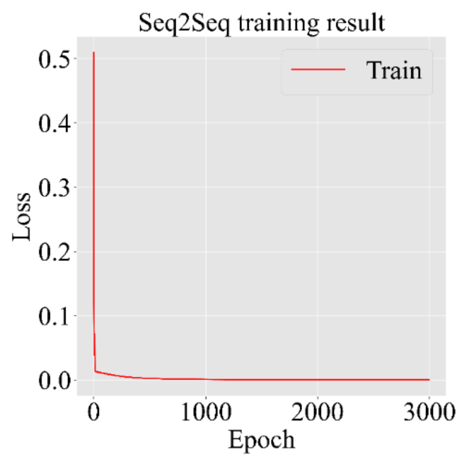
Figure 9 suggests that the model continues to train until it reached the 3000th epoch. The loss slowly converges to 0 after 300 epochs.
4.2. Results of Prediction Accuracy Comparison
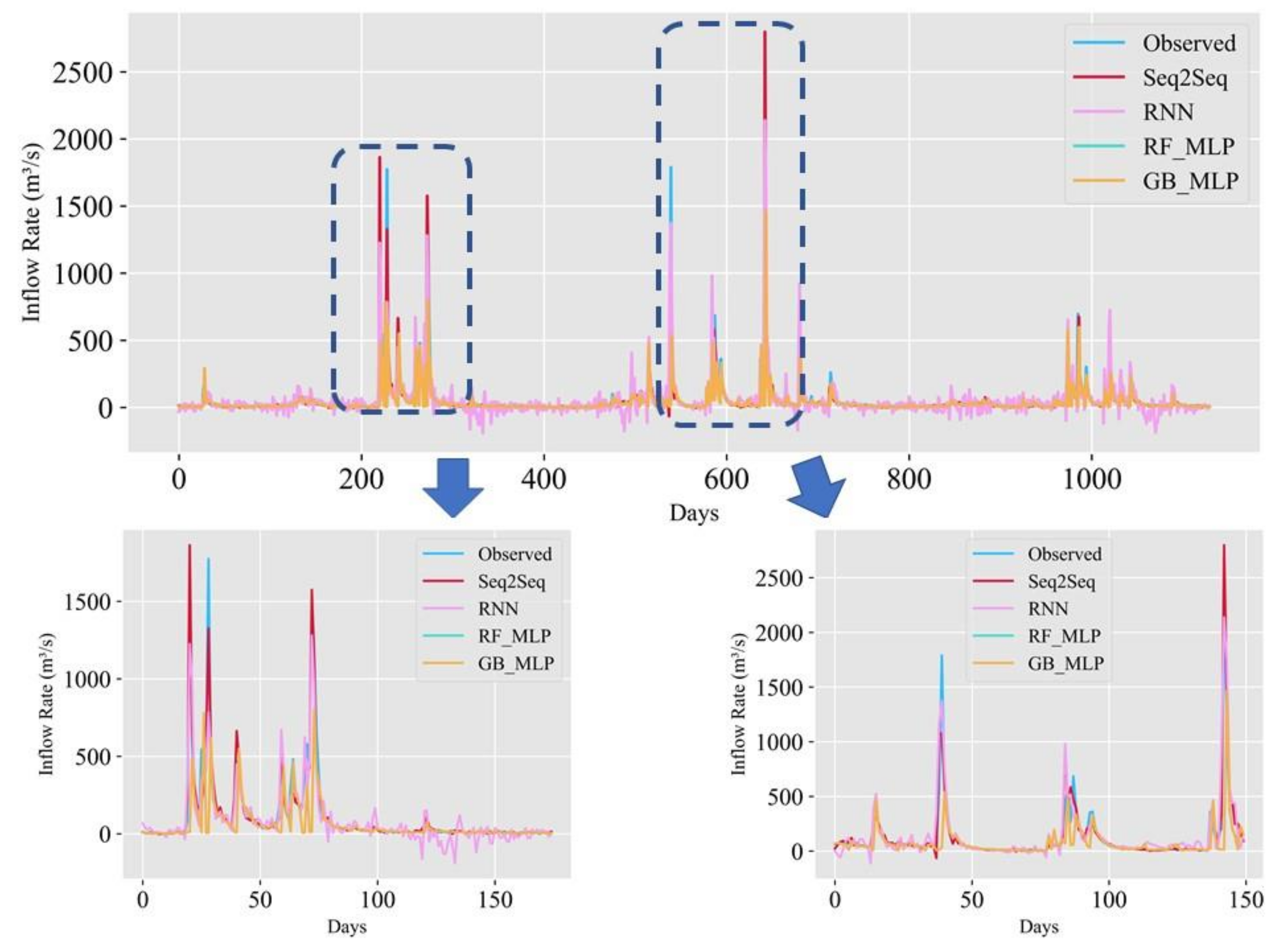
Figure 10 suggests that the proposed model and baseline models tend to follow the trend. However, RNN tends to frequently underestimate as if there are days with a negative inflow rate.
The results from Table 15 show that combining an ensemble model with MLP (Comb-ML) does not improve the prediction accuracy. Hong et al. [9] claimed that they combined MLP with an ensemble model because the MLP can predict most accurately when the inflow rate exceeds 100 m3/s, while an ensemble model can predict most accurately when the inflow rate is less than 100 m3/s. However, our experiment failed to support this claim. The RNN was the least performing model in this experiment. One possible explanation is that, unlike LSTM, the RNN model cannot store any critical information between the input and output. Changing the number of outputs per node can be helpful, and further research is required to improve the prediction accuracy of the RNN. The SVR and ensemble models had similar prediction accuracies.
Our model is the most accurate model compared with the baseline models. Compared with MLP, which is the most accurate baseline model, our model outperformed it on all metrics used for forecasting the day’s inflow. For predicting the next day’s inflow rate, the RMSE value decreased by 1.3, while the NSE value increased by 0.01. The only disadvantage of our model is that the MAE value was 0.16 higher than that of the MLP. In other words, our model can accurately forecast normal inflow, whereas MLP has better accuracy in predicting extreme forecasting events.
Table 16 compares the accuracy of our model with the RNN prediction result. Consequently, the RMSE value for the day forecasting was lowered by 56.17, and the MAE value was 38.57. The NSE value was 0.18 higher than that of the RNN. For the next day’s forecast, the RMSE and MAE values were lowered by 55.49 and 37.94, respectively. The NSE value increased by 0.17.
4.3. Ablation Study Analysis
Overall, the tested modifications prove that our model design helped to improve prediction accuracy. The modifications included changing the bidirectional LSTM to unidirectional LSTM for both the encoder and decoder, altering the activation function to tanh, and removing the heavy rain warning data.
As shown in Table 12, having bidirectional LSTM helps predict inflow accurately by learning patterns from past to present and present to past information. Changing the bidirectional LSTM to unidirectional LSTM lowers all prediction criteria values. Table 13 suggests that changing the activation function from tanh to SELU helps to increase the prediction accuracy. The SELU activation function enables the model to train under extreme conditions, such as flooding and drought, by self-normalizing to prevent exploding or vanishing gradient problems. By changing to the tanh activation function, the MAE value for forecasting the next day decreased by 0.08, and the NSE value decreased by 0.02 for predicting the day’s inflow.
As shown in Table 14, removing the warning data during training causes some prediction accuracy degradation. The RMSE value increased, but the MAE decreased for forecasting both days. The NSE value for forecasting the inflow rate for the same day was reduced by 0.01; however, the value was constant for the next day’s prediction.
4.4. Seq2Seq Model’s Performance Evaluation
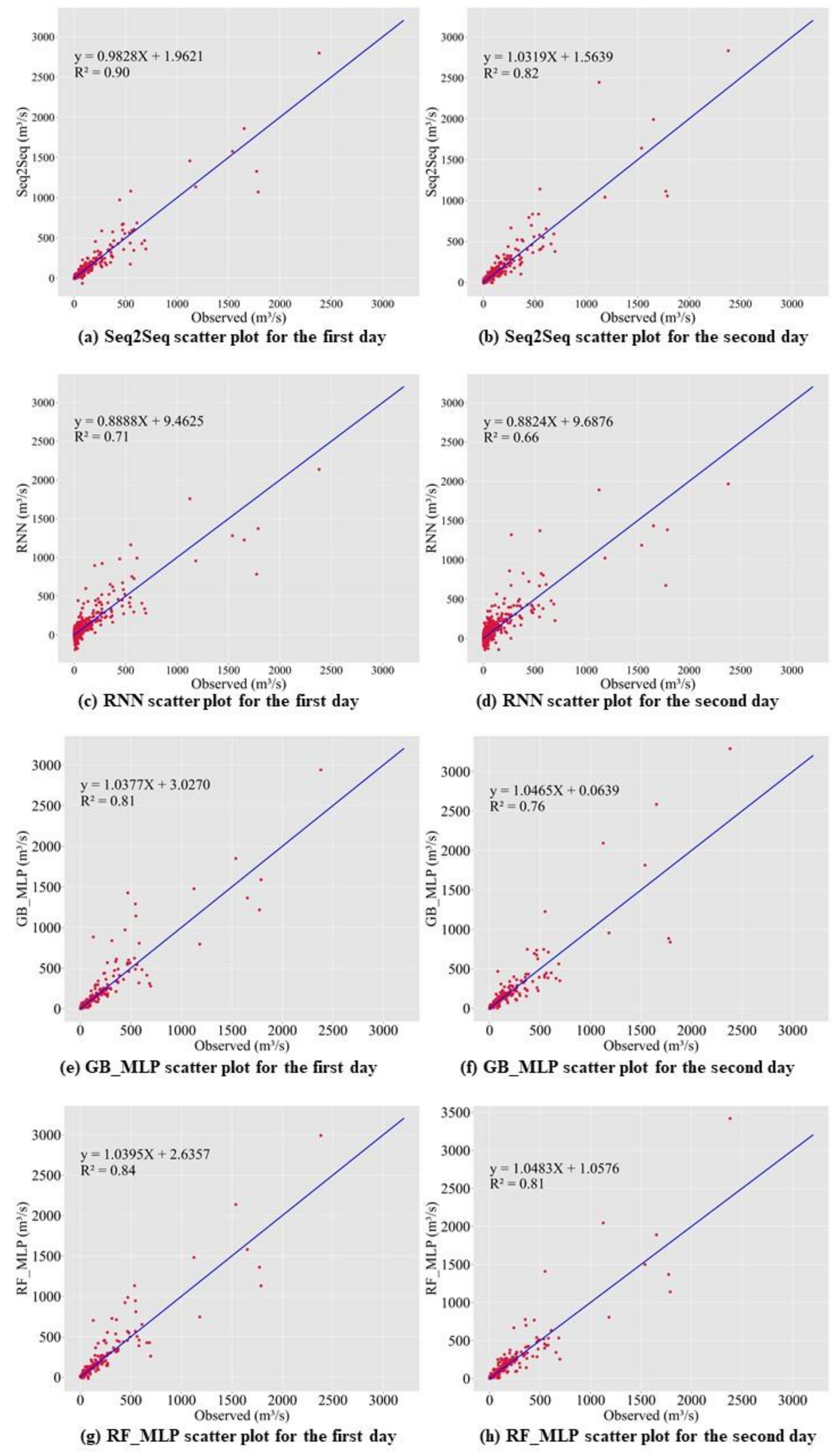
Figure 11 and Figure 12 suggest that our model is a good fit. Nearly all the data are close to the 45-degree line. Our model has the best performance for predicting the first day. RNN was the worst-performing model among the nine models. Scatter plots show that GB_MLP, RF_MLP, RNN, Seq2Seq shows the nearly equal predictive performance when the inflow rate is less than 1000 m3/s. RNN tends to underestimate when the inflow rate is greater than 1000 m3/s. GB_MLP, RF_MLP, and Seq2Seq tend to show similar predictive performance, but Seq2Seq tends to outperform other models when the inflow rate is greater than 1500 m3/s.
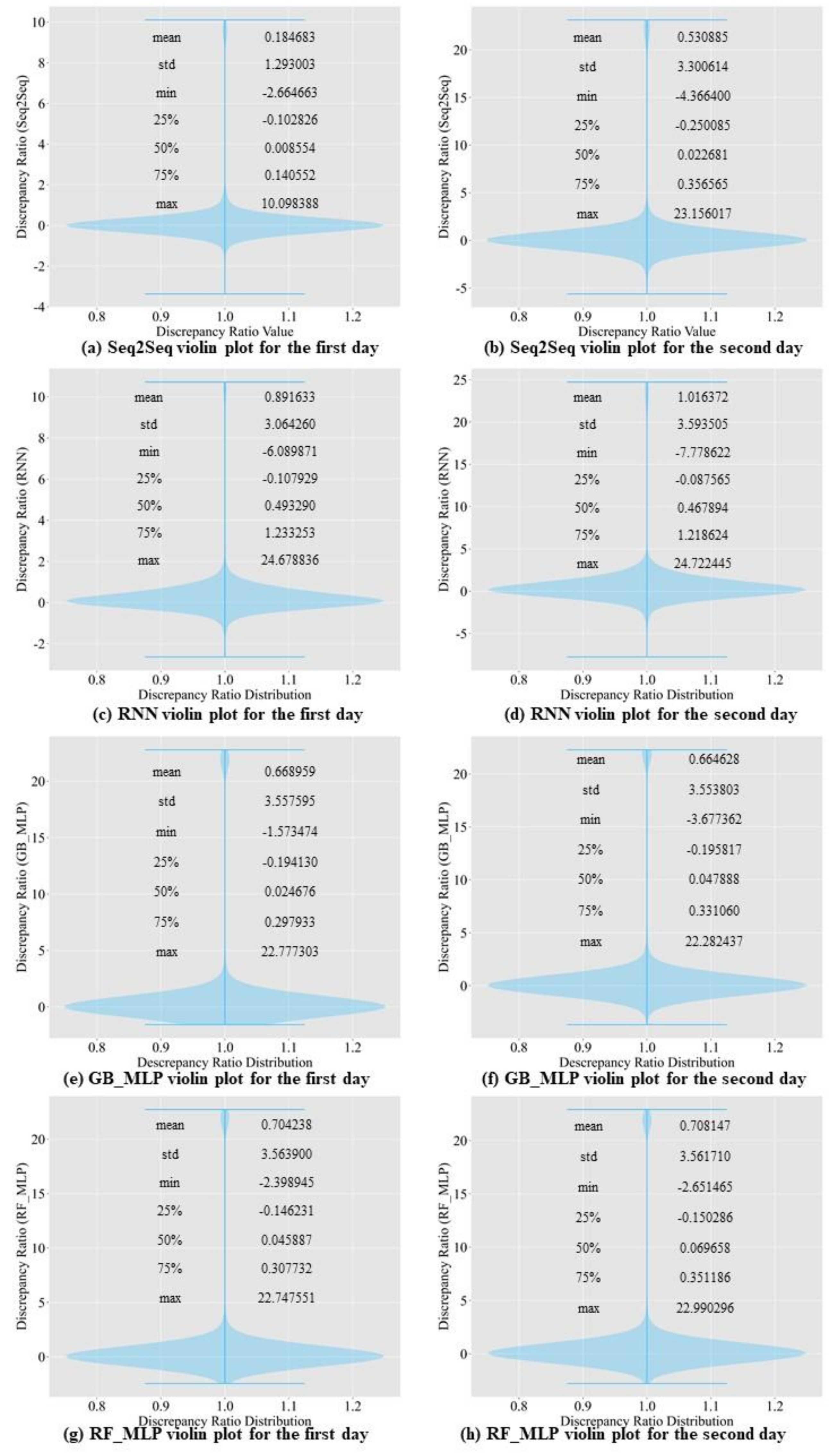
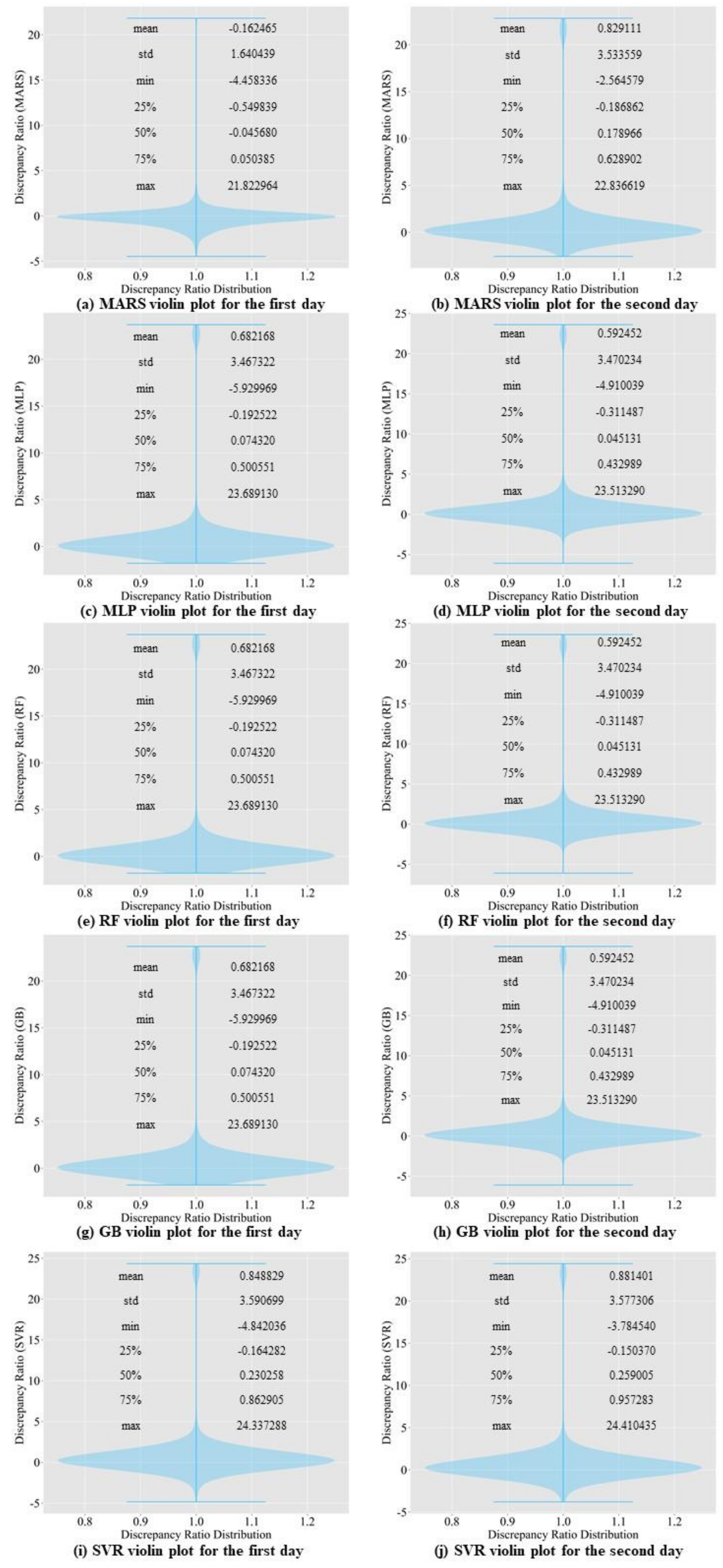
To evaluate the performance of the Seq2Seq model, we analyzed the discrepancy ratio. We analyzed with a test dataset. Equation (14) shows how to calculate the ratio. represents the predicted value, while represents the observed value. If the ratio is greater than 1, the model is overestimating. If the ratio is less than 1, the model is underestimating. If the ratio is equal to 1, the model shows the best prediction performance. We calculated the minimum, maximum, and average of the discrepancy ratio to analyze the proposed model. The test data contain 0 and cause the discrepancy ratio to become infinity. To avoid getting an infinity, we replaced 0 with . Figure 13 and Figure 14 suggest that all models tend to underestimate the inflow rate. Seq2Seq model is the model that has the least amount of errors. If we closely examine violin plots from Figure 13 and Figure 14, Seq2Seq data has less extreme discrepancy value than the other models. Even though all baseline models’ mean discrepancy is close to 1, extreme values are causing the mean discrepancy value to increase.
5. Conclusions
In this study, we propose a model that outperforms models from other studies. In addition, we set models from other studies as baseline models, namely MLP, random forest regressor, gradient boosting regressor, Comb-ML, and RNN models. We performed a grid search to determine the optimal hyperparameters for each model. Comb-ML combines an MLP model with an ensemble model, but its prediction performance was not better than that of the MLP model. The MLP model has the highest prediction accuracy, whereas RNN is the least accurate predictive model. The RNN model did not have the ability to retain important information for the prediction task. Therefore, the RNN uses all information without distinguishing critical information to predict the inflow rate. The prediction accuracy of our sequence-to-sequence model outperforms those of all baseline models. Only the next day’s MAE value for our model was higher than that of the MLP.
We propose the use of the SELU activation function with the LeCun normal kernel initializer for bidirectional LSTM to improve the prediction accuracy. This combination allowed stable training with self-normalizing features. Consequently, the model can accurately predict the inflow rate under extreme weather conditions, such as flooding and drought. In addition, bidirectional LSTM allows the model to learn the relationship from past to present and present to past. Therefore, the model requires more input information and predicts inflow more accurately than the baseline models.
Three cases were included in the ablation study. The first case involved removing the bidirectionality of the LSTM. The prediction accuracy decreased. The second case involved changing the SELU activation function to tanh. We observed a performance degradation in the inflow prediction. In the last case, warning data were excluded from training. The model returned less accurate predictions without the warning data. In conclusion, the ablation study proves that the bidirectionality of LSTM, a change in activation function, and the addition of warning data all contribute to the prediction accuracy.
The findings of this research show that the Seq2Seq model can be effective in predicting the inflow rate. Unlike physically based models, our model does not require detailed hydrological data for predicting the inflow rate. Therefore, our model is suitable for dams with lacking hydrological data. We also need to experiment with dams that contain abundant hydrological data to compare our model with physically based models. Lastly, we need to see how the Seq2Seq model performs if we include hydrological data to predict the inflow rate.
Author Contributions
Conceptualization, S.L. and J.K.; methodology, S.L. and J.K.; software, S.L.; validation, S.L. and J.K.; formal analysis, S.L. and J.K.; investigation, S.L. and J.K.; resources, S.L.; data curation, S.L.; writing—original draft preparation, S.L.; writing—review and editing, S.L. and J.K.; visualization, S.L.; supervision, J.K.; project administration, J.K.; funding acquisition, J.K. Both authors have read and agreed to the published version of the manuscript.
Funding
This work was supported by a National Research Foundation of Korea (NRF) grant funded by the Korean government (MSIT) (No. NRF-2019R1C1C1008174) and by the Ministry of Science and ICT (MSIT), Korea, under the ICT Creative Consilience program (IITP-2020-0-01821), supervised by the Institute for Information & Communications Technology Planning & Evaluation (IITP).
Institutional Review Board Statement
Not applicable.
Informed Consent Statement
Not applicable.
Data Availability Statement
The data and the results are available at https://github.com/samlee0326/Water.
Conflicts of Interest
The authors declare no conflict of interest.
References
- Park, J. Practical method for the 21st century water crisis using IWARM. J. Water Policy Econ. 2015, 24, 47–58. [Google Scholar]
- Shift in Water Resource Management Paradigm. K-water. 2012. Available online: https://www.kwater.or.kr/gov3/sub03/annoView.do?seq=1209&cate1=7&s_mid=54 (accessed on 6 September 2021).
- Park, J.Y.; Kim, S.J. Potential impacts of climate change on the reliability of water and hydropower supply from a multipurpose dam in South Korea. J. Am. Water Resour. Assoc. 2014, 50, 1273–1288. [Google Scholar] [CrossRef]
- Jung, S.; Lee, D.; Lee, K. “Prediction of River Water Level Using Deep-Learning Open Library. J. Korean Soc. Hazard Mitig. 2018, 18, 135. [Google Scholar] [CrossRef]
- Stern, M.; Flint, L.; Minear, J.; Flint, A.; Wright, S. Characterizing changes in streamflow and sediment supply in the Sacramento River Basin, California, using hydrological simulation program—FORTRAN (HSPF). Water 2016, 8, 432. [Google Scholar] [CrossRef] [Green Version]
- Ryu, J.; Jang, W.S.; Kim, J.; Choi, J.D.; Engel, B.A.; Yang, J.E.; Lim, K.J. Development of a watershed-scale long-term hydrologic impact assessment model with the asymptotic curve number regression equation. Water 2016, 8, 153. [Google Scholar] [CrossRef] [Green Version]
- Nyeko, M. Hydrologic modelling of data scarce basin with SWAT Model: Capabilities and limitations. Water Resour. Manag. 2015, 29, 81–94. [Google Scholar] [CrossRef]
- Park, M.K.; Yoon, Y.S.; Lee, H.H.; Kim, J.H. Application of recurrent neural network for inflow prediction into multi-purpose dam basin. J. Korea Water Resour. Assoc. 2018, 51, 1217–1227. [Google Scholar]
- Hong, J.; Lee, S.; Bae, J.H.; Lee, J.; Park, W.J.; Lee, D.; Kim, J.; Lim, K.J. Development and Evaluation of the Combined Machine Learning Models for the Prediction of Dam Inflow. Water 2020, 12, 2927. [Google Scholar] [CrossRef]
- Babei, M.; Ehsanzadeh, E. Artificial Neural Network and Support Vector Machine Models for Inflow Prediction of Dam Reservoir (Case Study: Zayandehroud Dam Reservoir). Water Resour. Manag. 2019, 33, 2203–2218. [Google Scholar] [CrossRef]
- Yu, X.; Wang, Y.; Wu, L.; Chen, G.; Wang, L.; Qin, H. Comparison of support vector regression and extreme gradient boosting for decomposition-based data-driven 10-day streamflow forecasting. J. Hydrol. 2020, 582, 124293. [Google Scholar] [CrossRef]
- Zhang, D.; Lin, J.; Peng, Q.; Wang, D.; Yang, R.; Sorooshian, S.; Liu, X.; Zhuang, J. Modeling and simulating of reservoir operation using the artificial neural network, support vector regression, deep learning algorithm. J. Hydrol. 2018, 565, 720–736. [Google Scholar] [CrossRef] [Green Version]
- Seo, Y.; Choi, E.; Yeo, W. Reservoir Water Level Forecasting Using Machine Learning Models. J. Korean Soc. Agric. Eng. 2017, 59, 97–110. [Google Scholar]
- Liao, S.; Liu, Z.; Liu, B.; Cheng, C.; Jin, X. Multistep-ahead daily inflow forecasting using the ERA-nterim reanalysis data set based on gradient-boosting regression trees. Hydrol. Earth Syst. Sci. 2020, 24, 2343–2363. [Google Scholar] [CrossRef]
- Le, X.-H.; Ho, H.V.; Lee, G.; Jung, S. Ap plication of long short-term memory (LSTM) neural network for flood forecasting. Water 2019, 11, 1387. [Google Scholar] [CrossRef] [Green Version]
- Mok, J.Y.; Choi, J.H.; Moon, Y. Prediction of multipurpose dam inflow using deep learning. J. Korea Water Resour. Assoc. 2020, 53, 97–105. [Google Scholar]
- Saberi-Movahed, F.; Mohammadifard, M.; Mehrpooya, A.; Rezaei-Ravari, M.; Berahmand, K.; Rostami, M.; Karami, S.; Najafzadeh, M.; Hajinezhad, D.; Jamshidi, M.; et al. Decoding Clinical Biomarker Space of COVID-19: Exploring Matrix Factorization-based Feature Selection Methods. medRxiv 2021, preprint, 1–51. [Google Scholar]
- Najafzadeh, M.; Niazmardi, S. A Novel Multiple-Kernel Support Vector Regression Algorithm for Estimation of Water Quality Parameters. Nat. Resour. Res. 2021, 17, 1–15. [Google Scholar]
- Amiri-Ardakani, Y.; Najafzadeh, M. Pipe Break Rate Assessment While Considering Physical and Operational Factors: A Methodology based on Global Positioning System and Data-Driven Techniques. Water Resour. Manag. 2021, in press. [Google Scholar] [CrossRef]
- Adnan, R.M.; Liang, Z.; El-Shafie, A.; Zounemat-Kermani, M.; Kisi, O. Prediction of Suspended Sediment Load Using Data-Driven Models. Water 2019, 11, 2060. [Google Scholar] [CrossRef] [Green Version]
- Adnan, R.M.; Liang, Z.; Parmar, K.S.; Soni, K.; Kisi, O. Modeling monthly streamflow in mountainous basin by MARS, GMDHNN and DENFIS using hydroclimatic data. Neural Comput. Appl. 2020, 33, 2853–2871. [Google Scholar] [CrossRef]
- Adnan, R.M.; Khosravinia, P.; Karimi, B.; Kisi, O. Prediction of hydraulics performance in drain envelopes using Kmeans based multivariate adaptive regression spline. Appl. Soft Comput. J. 2020, 100, 2021. [Google Scholar]
- Adnan, R.M.; Liang, Z.; Trajkovic, S.; Zounemat-Kermani, M.; Li, B.; Kisi, O. Daily streamflow prediction using optimally pruned extreme learning machine. J. Hydrol. 2019, 577, 123981. [Google Scholar] [CrossRef]
- Adnan, R.M.; Liang, Z.; Heddam, S.; Zounemat-Kermani, M.; Kisi, O.; Li, B. Least square support vector machine and multivariate adaptive regression splines for streamflow prediction in mountainous basin using hydro-meteorological data as inputs. J. Hydrol. 2020, 586, 124371. [Google Scholar] [CrossRef]
- Kwin, C.T.; Talei, A.; Alaghmand, S.; Chua, L.H. Rainfall-runoff modeling using Dynamic Evolving Neural Fuzzy Inference System with online learning. Procedia Eng. 2016, 154, 1103–1109. [Google Scholar] [CrossRef] [Green Version]
- Yuan, X.; Chen, C.; Lei, X.; Yuan, Y.; Adnan, R.M. Monthly runoff forecasting based on LSTM–ALO model. Stoch. Environ. Res. Risk Assess. 2018, 32, 2199–2212. [Google Scholar] [CrossRef]
- Adnan, R.M.; Yuan, X.; Kisi, O.; Anam, R. Improving Accuracy of River Flow Forecasting Using LSSVR with Gravitational Search Algorithm. Adv. Meteorol. 2017, 2017, 1–23. [Google Scholar] [CrossRef]
- Shortridge, J.E.; Guikema, S.D.; Zaitchik, B.F. Machine learning methods for empirical streamflow simulation: A comparison of model accuracy, interpretability, and uncertainty in seasonal watersheds. Hydrol. Earth Syst. Sci. 2016, 20, 2611–2628. [Google Scholar] [CrossRef] [Green Version]
- Korea National Committee on Large Dams. Available online: http://www.kncold.or.kr/eng/ds4_1.html (accessed on 15 March 2021).
- Dam Operation Status. Available online: https://www.water.or.kr/realtime/sub01/sub01/dam/.hydr.do?seq=1408&p_group_seq=1407&menu_mode=2 (accessed on 15 March 2021).
- Korea Meteorological Administration (KMA). Available online: http://kma.go.kr/home/index.jsp (accessed on 12 January 2021).
- Weather Warning Status. Available online: http://www.kma.go.kr/HELP/html/help_wrn001.jsp (accessed on 12 January 2021).
- Woo, W.; Moon, J.; Kim, N.W.; Choi, J.; Kim, K.S.; Park, Y.S.; Jang, W.S.; Lim, K.J. Evaluation of SATEEC Daily R Module using Daily Rainfall. J. Korean Soc. Water Environ. 2010, 26, 841–849. [Google Scholar]
- Hochreiter, S.; Schmidhuber, J. Long short-term memory. Neural Comput. 1997, 9, 1735–1780. [Google Scholar] [CrossRef] [PubMed]
- Schuster, M.; Paliwal, K.K. Bidirectional recurrent neural networks. IEEE Trans. Signal Process. 1997, 45, 2673–2681. [Google Scholar] [CrossRef] [Green Version]
- Persio, L.D.; Honchar, O. Analysis of Recurrent Neural Networks for Short-Term. AIP Conf. 2017, 1906, 190006. [Google Scholar]
- Althelaya, K.A.; El-Alfy, E.S.M.; Mohammed, S. Evaluation of Bidirectional LSTM for Short- and Long-Term Stock Market Prediction. In Proceedings of the International Conference on Information and Communication Systems (ICICS), Irbid, Jordan, 3–5 April 2018; pp. 151–156. [Google Scholar]
- Suyskever, I.; Vinyals, O.; Le, Q.V. Sequence to sequence learning with neural networks. In Proceedings of the Neural Information Processing Systems, Montreal, QC, Canada, 8–13 December 2014; Volume 2, pp. 3104–3112. [Google Scholar]
- Smola, A.J.; Schölkopf, B. A tutorial on support vector regression. Stat. Comput. 2004, 14, 199–222. [Google Scholar] [CrossRef] [Green Version]
- Ho, T.K. Random Decision Forests. In Proceedings of the 3rd International Conference on Document Analysis and Recognition, Montreal, QC, Canada, 14–16 August 1995; pp. 278–282. [Google Scholar]
- Géron, A. Hands-On Machine Learning with Scikit-Learn, Keras & Tensorflow; O’Reilly: Sebastopol, CA, USA, 2020; pp. 254–255. [Google Scholar]
- Schapire, R.E. A Brief Introduction to Boosting. In Proceedings of the 16th International Joint Conference on Artificial Intelligence (IJCAI), Stockholm, Sweden, 31 July–6 August 1999; pp. 1401–1406. [Google Scholar]
- Rosenblatt, F. The perceptron: A probabilistic model for information storage and organization in the brain. Psychol. Rev. 1958, 65, 386–408. [Google Scholar] [CrossRef] [PubMed] [Green Version]
- Rumelhart, D.E.; Hinton, G.E.; Williams, R.J. Learning Internal Representations by Error Propagation. In Parallel Distributed Processing: Explorations in the Microstructure of Cognition: Foundations; MIT Press: Cambridge, MA, USA, 1987; pp. 318–362. [Google Scholar]
- Friedman, J.H. Multivariate adaptive regression splines. Ann. Stat. 1991, 19, 1–67. [Google Scholar] [CrossRef]
- Py-Earth. Available online: https://contrib.scikit-learn.org/py-earth/content.html# (accessed on 12 August 2021).
- Klambauer, G.; Unterthiner, T.; Mayr, A. Self-Normalizing Neural Networks. In Proceedings of the 31st International Conference on Neural Information Processing Systems, Long Beach, CA, USA, 4–9 December 2017; pp. 972–981. [Google Scholar]
Figure 1.
Time series data of dam inflow and weather.

Figure 2.
Heat map of correlation coefficients of variables.

Figure 3.
Violin plot for training and testing data.

Figure 4.
Structure of LSTM.

Figure 5.
Structure of a bidirectional LSTM.

Figure 6.
Seq2Seq model schematics.

Figure 7.
A detailed schematics of a Seq2Seq’s bidirectional LSTM module.

Figure 8.
The overall training procedure for Seq2Seq model.

Figure 9.
Graph for Seq2Seq model training loss.

Figure 10.
Time variation graph for the proposed model RNN, RF_MLP and GB_MLP.

Figure 11.
Scatter plots for predicting inflow rate with the proposed model and based models.

Figure 12.
Scatter plot for predicting the inflow rate with baseline models.

Figure 13.
Violin plot for the discrepancy ratio for the proposed model and baseline models.

Figure 14.
Violin plot for the discrepancy ratio for baseline models.


Table 1.
Input data for the proposed and baseline models.
| Input Variable | Output Variable | |
|---|---|---|
| Weather data for the last seven days | Inflow (t − 7) | |
| Inflow (t − 6) | ||
| Inflow (t − 1) | ||
| min_temperature (t − 7), min_temperature (t − 6), min_temperature (t − 1) | ||
| max_temperature (t − 7), max_temperature (t − 6), max_temperature (t − 1) | ||
| precipitation (t − 7), | ||
| precipitation (t − 6), | ||
| precipitation (t − 1) | ||
| wind (t − 7), | Inflow of the day: Inflow (t), | |
| wind (t − 6), | Inflow of the next day: Inflow (t + 1) | |
| wind (t − 1) | ||
| solar_radiation (t − 7), solar_radiation (t − 6), olar_radiation (t − 1) | ||
| humidity (t − 7) | ||
| humidity (t − 6) | ||
| humidity (t − 1) | ||
| heavy_rain_warn (t − 7), heavy_rain_warn (t − 6) | ||
| heavy_rain_warn (t − 1) | ||
| Forecasted data | precipitation (t) | |
| precipitation (t + 1) |
Note: The ‘Inflow’, ‘min_temperature’, ‘max_temperature’, ‘precipitation’, ‘wind’, ‘solar’, ‘humidity’, ’ heavy_rain_warn’, ‘(t − 7)’, ‘(t − 6)’, ‘(t − 1)’, ‘(t)’, and ‘(t + 1)’ are the daily dam inflow, minimum temperature of the day, the maximum temperature of the day, precipitation of the day, average wind speed of the day, total radiation of the day, relative humidity of the day, number of heavy rain warning of the day, seven days ago, six days ago, one day ago, the day, and the next day, respectively.
Table 2.
Hyperparameters to determine the optimal values for support vector regressor.
| Hyperparameter | Value |
|---|---|
| kernel | poly, rbf |
| degree | 2, 3, 4, 5 |
| gamma | scale, auto |
Table 3.
Hyperparameters to determine the optimal values for random forest regressor.
| Hyperparameter | Value |
|---|---|
| n_estimators | 100, 200, 500 |
| max_features | 2, 3, 4, 5 |
| criterion | mse, mae |
Table 4.
Hyperparameters to find the optimal values for gradient boosting regressor.
| Hyperparameter | Value |
|---|---|
| loss | ls, lad, huber, quantile |
| learning_rate | 0.1, 0.01, 0.001 |
| n_estimators | 100, 200, 300 |
| criterion | friedman_mse, mse. mae |
Table 5.
Hyperparameters to determine the optimal values for multilayer perceptron regressor.
| Hyperparameter | Value |
|---|---|
| hidden_layer_sizes | (30, 30, 30), (50, 50, 50), (100, 100) |
| activation | Identity, logistic, tanh, relu |
| solver | lbfgs, sgd, adam |
| batch_size | 32, 64, 128 |
| learning_rate | Constant, invscaling, adaptive |
| shuffle | True, False |
Table 6.
Hyperparameters for the recurrent neural network grid search.
| Hyperparameter | Value |
|---|---|
| Learning rate | 0.1, 0.01, 0.001 |
| Batch size | 64, 128, 256 |
Table 7.
Hyperparameters for bidirectional LSTM sequence-to-sequence model grid search.
| Hyperparameter | Value |
|---|---|
| Learning rate | 0.1, 0.01, 0.001 |
| Batch size | 64, 128, 256 |
| Number of output units | |
| per bidirectional LSTM | 59,100,118,177 |
Table 8.
Prediction accuracy results for baseline models.
| Baseline Model | Prediction Time | RMSE | MAE | NSE |
|---|---|---|---|---|
| RNN | T | 100.34 | 53.51 | 0.78 |
| T + 1 | 104.08 | 55.05 | 0.77 | |
| MLP | T | 53.49 | 16.74 | 0.94 |
| T + 1 | 59.89 | 16.95 | 0.93 | |
| SVR | T | 63.78 | 26.06 | 0.92 |
| T + 1 | 73.12 | 28.80 | 0.89 | |
| Random Forest Regressor | T | 66.63 | 15.76 | 0.91 |
| T + 1 | 58.21 | 15.95 | 0.93 | |
| Gradient Boosting Regressor | T | 76.90 | 16.71 | 0.90 |
| T + 1 | 64.78 | 17.21 | 0.93 | |
| Comb -ML (RF_MLP) | T | 69.79 | 16.44 | 0.92 |
| T + 1 | 71.01 | 16.80 | 0.92 | |
| Comb -ML (GB_MLP) | T | 69.39 | 16.73 | 0.92 |
| T + 1 | 71.17 | 16.97 | 0.92 | |
| MARS | T | 71.68 | 21.88 | 0.907 |
| T + 1 | 73.37 | 25.48 | 0.902 |
Table 9.
Hyperparameters for baseline models.
| MLP | Support Vector Regressor | ||
|---|---|---|---|
| Hyperparameter | Value | Hyperparameter | Value |
| activation | logistic | degree | 2 |
| batch_size | 32 | gamma | auto |
| Hidden_layer_size | (100, 100, 100) | kernel | poly |
| learning_rate | constant | ||
| shuffle | False | ||
| solver | lbfgs | ||
| Random Forest Regressor | Gradient Boosting Regressor | ||
| Hyperparameter | Value | Hyperparameter | Value |
| criterion | mse | criterion | mse |
| max_features | auto | learning_rate | 0.1 |
| n_estimators | 100 | loss | ls |
| n_estimators | 300 | ||
| RNN | |||
| Hyperparameter | Value | ||
| Batch Size | 64 | ||
| Learning rate | 0.1 | ||
Table 10.
Hyperparameter values for our model.
| Our Proposed Model | |
|---|---|
| Hyperparameter | Value |
| Batch size | 256 |
| Learning rate | 0.001 |
| Number of output units per bidirectional LSTM | 177 |
Table 11.
Prediction accuracy results of our proposed model and the MLP.
| Sequence-to-Sequence Model (Our Model) | MLP | |||||
|---|---|---|---|---|---|---|
| RMSE | MAE | NSE | RMSE | MAE | NSE | |
| T | 44.17 | 14.94 | 0.96 | 53.49 | 16.74 | 0.94 |
| T + 1 | 58.59 | 17.11 | 0.94 | 59.89 | 16.95 | 0.93 |
Table 12.
Prediction accuracy results after removing bidirectionality from LSTM.
| Sequence-to-Sequence Model (Unidirectional LSTM) | Sequence-to-Sequence Model (Control) | |||||
|---|---|---|---|---|---|---|
| RMSE | MAE | NSE | RMSE | MAE | NSE | |
| T | 54.90 | 16.23 | 0.94 | 44.17 | 14.94 | 0.96 |
| T + 1 | 74.12 | 19.29 | 0.90 | 58.59 | 17.11 | 0.94 |
Table 13.
Prediction accuracy results after changing activation function to tanh.
| Sequence-to-Sequence Model (Activation Function: Tanh) | Sequence-to-Sequence Model (Control) | |||||
|---|---|---|---|---|---|---|
| RMSE | MAE | NSE | RMSE | MAE | NSE | |
| T | 58.38 | 15.62 | 0.94 | 44.17 | 14.94 | 0.96 |
| T + 1 | 61.04 | 17.03 | 0.94 | 58.59 | 17.11 | 0.94 |
Table 14.
Prediction accuracy results after excluding warning data.
| Sequence-to-Sequence Model (No Warning Data) | Sequence-to-Sequence Model (Control) | |||||
|---|---|---|---|---|---|---|
| RMSE | MAE | NSE | RMSE | MAE | NSE | |
| T | 54.19 | 14.57 | 0.95 | 44.17 | 14.94 | 0.96 |
| T + 1 | 60.67 | 16.59 | 0.94 | 58.59 | 17.11 | 0.94 |
Table 15.
Prediction accuracy result of the proposed model, Comb- ML and RNN.
| Models | Metrics | |||
|---|---|---|---|---|
| RMSE | MAE | NSE | ||
| Our model (Seq2Seq) | T | 44.17 | 14.94 | 0.96 |
| T + 1 | 58.59 | 17.11 | 0.94 | |
| Comb-ML (RF_MLP) | T | 69.79 | 16.44 | 0.92 |
| T + 1 | 71.01 | 16.80 | 0.92 | |
| Comb-ML (RF_MLP) | T | 69.39 | 16.73 | 0.92 |
| T + 1 | 71.17 | 16.97 | 0.92 | |
| RNN | T | 100.34 | 53.51 | 0.78 |
| T + 1 | 104.08 | 55.05 | 0.77 | |
Table 16.
Prediction accuracy results of our proposed model and the RNN.
| Sequence-to-Sequence Model (Our Model) | RNN | |||||
|---|---|---|---|---|---|---|
| RMSE | MAE | NSE | RMSE | MAE | NSE | |
| T | 44.17 | 14.94 | 0.96 | 100.34 | 53.51 | 0.78 |
| T + 1 | 58.59 | 17.11 | 0.94 | 104.08 | 55.05 | 0.77 |
Publisher’s Note: MDPI stays neutral with regard to jurisdictional claims in published maps and institutional affiliations. |
© 2021 by the authors. Licensee MDPI, Basel, Switzerland. This article is an open access article distributed under the terms and conditions of the Creative Commons Attribution (CC BY) license (https://creativecommons.org/licenses/by/4.0/).
Share and Cite
MDPI and ACS Style
Lee, S.; Kim, J. Predicting Inflow Rate of the Soyang River Dam Using Deep Learning Techniques. Water 2021, 13, 2447. https://doi.org/10.3390/w13172447
AMA Style
Lee S, Kim J. Predicting Inflow Rate of the Soyang River Dam Using Deep Learning Techniques. Water. 2021; 13(17):2447. https://doi.org/10.3390/w13172447
Chicago/Turabian StyleLee, Sangwon, and Jaekwang Kim. 2021. "Predicting Inflow Rate of the Soyang River Dam Using Deep Learning Techniques" Water 13, no. 17: 2447. https://doi.org/10.3390/w13172447
Note that from the first issue of 2016, this journal uses article numbers instead of page numbers. See further details here.