Towards a Comprehensive Assessment of Statistical versus Soft Computing Models in Hydrology: Application to Monthly Pan Evaporation Prediction

Abstract

This paper evaluates six soft computational models along with three statistical data-driven models for the prediction of pan evaporation (EP). Accordingly, improved kriging—as a novel statistical model—is proposed for accurate predictions of EP for two meteorological stations in Turkey. In the standard kriging model, the input data nonlinearity effects are increased by using a nonlinear map and transferring input data from a polynomial to an exponential basic function. The accuracy, precision, and over/under prediction tendencies of the response surface method, kriging, improved kriging, multilayer perceptron neural network using the Levenberg–Marquardt (MLP-LM) as well as a conjugate gradient (MLP-CG), radial basis function neural network (RBFNN), multivariate adaptive regression spline (MARS), M5Tree and support vector regression (SVR) were compared. Overall, all the applied models were highly capable of predicting monthly EP in both stations with a mean absolute error (MAE) < 0.77 mm and a Willmott index (d) > 0.95. Considering periodicity as an input parameter, the MLP-LM provided better results than the other methods among the soft computing models (MAE = 0.492 mm and d = 0.981). However, the improved kriging method surpassed all the other models based on the statistical measures (MAE = 0.471 mm and d = 0.983). Finally, the outcomes of the Mann–Whitney test indicated that the applied soft computational models do not have significant superiority over the statistical ones (p-value > 0.65 at α = 0.01 and α = 0.05).

1. Introduction

One of the key elements of water resources management and hydrological projects is to estimate the evaporation in a given region. This is even more important in managing water resources in arid and semi-arid regions [1]. Some researchers have applied the Budyko framework, which is a straightforward model that considers only rainfall and potential evaporation as the required input for simulating and controlling various water management plans [2,3]. Simply, knowing the accurate amount of the evaporation is essential for water resources management projects.

Researchers have applied different approaches for modeling pan evaporation (EP) and evapotranspiration in the literature classified as (i) physically-based combination models that take into account mass and energy conservation principles; (ii) semi-physical models that use either mass or energy conservation; and (iii) data-driven models including soft computing and statistical techniques [4,5,6]. The shortage of EP data (temporally or spatially) is a major problem in some areas because it is difficult and expensive to install evaporation pans. In these cases, applying data-driven and soft computing models for estimating water evaporation is an effective and appropriate approach [7,8,9]. The accuracy of modeling approaches is the most important parameter to take into account.

Several researchers have used climatic variables to estimate EP values [10,11]. Climate-based approaches are appropriate methods when provided with specific climatic data, which cannot always be easily obtained from a determined area. Similarly, data-driven approaches, including computational intelligence and machine learning are also suitable for estimating the EP. Recently, regular hybrid and integrative data-driven models (e.g., artificial neural networks (ANN) as well as support vector machine (SVM) and adaptive neuro-fuzzy inference systems (ANFIS)) have been used for estimating the EP [7,12,13,14,15,16,17,18,19,20].

Tabari et al. [21] estimated the daily EP of a region by using different methods (ANNs and multivariate nonlinear regression (MNLR)) and concluded that ANN was more accurate than MNLR. Kişi et al. [22] applied three soft computing models, such as M5tree, ANN, and chi-squared automatic interaction, to predict the daily EPs in Turkey. They reported that the ANN model performed better than the two others. Tezel and Buyukyildiz [23] investigated the usability of ANNs and ε-SVR to estimate monthly EP. According to the performance criteria, the ANN algorithms and ε-SVR had the same performance. Tezel and Buyukyildiz [23] compared the accuracy of SVM basis ε-support vector regression, radial basis function (RBFNN), and multilayer perceptron ANN (MLPNN), and showed that the latter provided the most accurate results. Keshtegar and Kisi [24] proposed the modified response surface method (RSM) and modified RSMs have been compared with ANFIS and M5Tree. Wang et al. [25] investigated the capabilities of ANFIS, M5Tree, and fuzzy genetic (FG) for six stations in the Yangtze River Basin. The results stated that the FG model generally produced better results. In another study, Wang et al. [26] compared the abilities of FG, SVR, MARS, M5Tree, and multiple linear regression (MLR). The overall results indicated that the soft computing models generally performed better than the regression methods. Ghorbani et al. [27] applied a hybrid MLPNN for daily EP prediction at two stations. The results showed that the MLPNN model provided better performance compared to the SVM model. Majhi et al. [28] applied a deep ANN model and compared it with the traditional MLPNN for three areas of the Chhattisgarh State in India. The findings of the study showed that the deep ANN model was more accurate than the traditional MLPNN. The abilities of ANN and extreme learning machine (ELM) models have been compared in predicting EP for two stations in Algeria by Sebbar et al. [29]. The results indicated that the ELM could be successfully used to estimate the daily EP [29]. Al-Mukhtar [30] investigated the applicability of quantile regression forest for EP prediction in arid areas. In comparison to conventional NNs and linear regression models, the applied quantile regression forest provided better results. Mohammadi et al. [31] predicted monthly EP using integrative ANFIS, MLP and RBNN models for two stations in Iran. The results showed that the integrative ANFIS model acted better compared to the MLP and RBNN. Yaseen et al. [32] applied several machine learning models, including ANN, classification and regression tree (CART), gene expression programming and SVM for predicting EP in arid and semi-arid areas. The findings of the study indicated that the SVM was superior to the other applied models.

A literature review related to the kriging approach revealed that it has never been used to predict PE. However, this method was applied for the prediction of solar radiation [33] and the daily total dissolved gas in aquatic systems concentration by Heddam et al. [34]. The kriging interpolation, which is a flexible regression tool for approximating any nonlinear problem, can be introduced as a potential method for providing accurate EP predictions.

Indeed, soft computing techniques have provided satisfactory results in EP prediction [35]. The majority of EP modeling reported the superiority of soft computing models over statistical models [21,26,36]. The main objective of this study is to challenge the capability of soft computing techniques versus statistical data-driven models.

The present study investigates the accuracy of six soft computing methods, including M5tree, MARS, SVR, RBFNN, Levenberg–Marquardt perceptron ANN and conjugate gradient perceptron ANN and compares them with three different statistical approaches, RSM, kriging, and improved kriging. In improved kriging, the basic functions are transferred from polynomial to exponential functions to estimate monthly EP. In kriging models, the second-order polynomial function is applied as regressed function to predict nonlinear challenges. This function may not have predicted an accurate result for complex problems such as EP. Thus, novel improved modeling is parented to enhance the regressed function applied in original kriging. It uses a nonlinear transformation as an exponential map for input variables of the EP predictions as a complex engineering problem with nonlinear effect that the accurate results in the modeling process is a cap for prediction of the statistical regression approaches such as kriging and RSM models.

To our best knowledge, similar studies have not been carried out in applying the above-mentioned methods for the estimation of EP. The subsequent parts of the rest of the paper are organized as follows: In Section 2, the two stations are introduced, and the data sets are presented. The third section deals with nine modeling methods applied in statistical and soft computing approaches. The results of the predicted EP are presented and compared in the fourth section. The fifth section of the paper deals with the hypothesis testing and relevant discussion. Finally, the last section provides the concluding remarks of the present work.

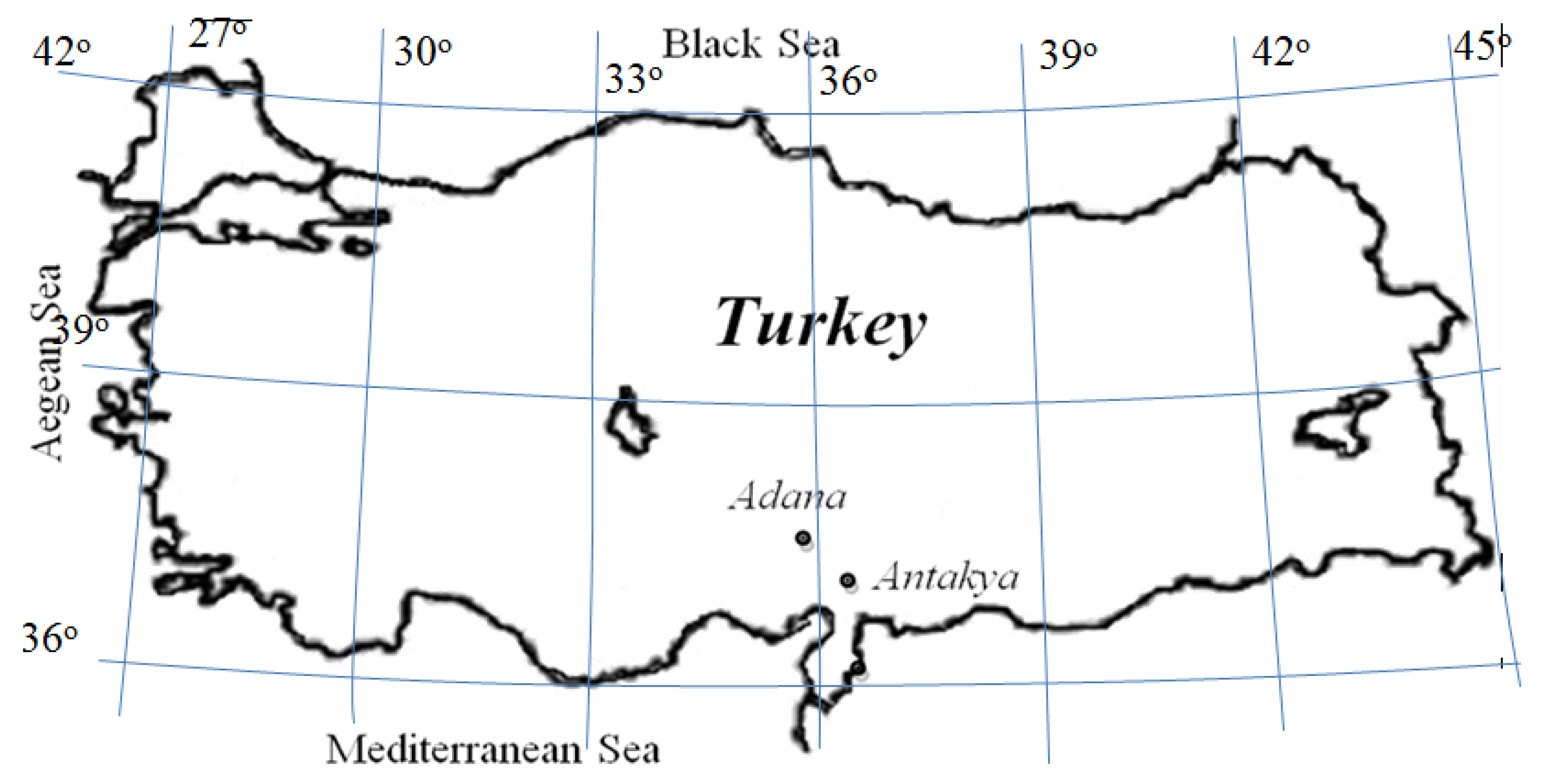
2. Case Study and Dataset

The input parameters for this study are monthly climatic data such as solar radiation (SR, as Langley), sunshine hours (HS), relative humidity (RH), wind speed (WS as m/s) as well as the minimum (Tmin as °C) and maximum temperature (Tmax as °C). Two stations in the Eastern Mediterranean Region as Adana (latitude 37.22° N, longitude 35.40° E and altitude 20 m) and Antakya (latitude 36.33° N, longitude 36.30° E and altitude 100 m) were selected for the comparing modeling results. The map of the study area is illustrated in Figure 1. The studied area has a climate with cool and rainy winters, and moderately hot and dry summers and it receives yearly rainfall amounts of between 580 and 1300 mm. Data were gathered from the Turkish State Meteorological Service (TSMS) having a modernized calibration center. The calibration center was accredited by the Turkish Accreditation Agency to ensure the measurements’ reliability and to provide the validity of the measurements’ quality around the world. Temperature, RH, and WS calibration laboratories are accredited with TS EN ISO/IEC 17025 standards and work in accordance with this standard. Global radiation and wind direction data are also in accordance with the TS EN ISO/IEC 17025 standards. The evaporimeter used for obtaining pan evaporation in Turkey is the US Weather Bureau Class A pan. The raw datasets were directly utilized in the presented study without pre-processing. The available data period covers September 1981 to March 2016 for Adana and from October 1983 to December 2010 for Antakya. There is no gap in the data.

In Figure 2, the general characteristics of the independent variables and the target value for the (a) Adana and (b) Antakya stations are shown using the box-whisker plot and related correlation values. These plots graphically depict the variability of each parameter in terms of minimum, quartiles, and maximum values. Moreover, outliers are plotted as individual points.

The Pearson correlation coefficient was applied to analyze the effects of Tmax, RH, WS, SR, and HS on EP. It can be seen from Figure 2 that there were high correlations between EP, Tmin, Tmax, SR, and HS for both Stations. It is worth noting that the wind speed showed high correlation with EP for the Antakya Station (correlation = 0.804), whereas the reciprocal value of the WS correlation for the Adana Station is much lower (correlation = 0.245).

For both of the Stations, the correlation between the relative humidity (RH) and the EP was weaker than the other parameters. However, in the Antakya Station, the correlation value of RH is negative, which implies that the increase in relative humidity might lead to a decrease in EP. The main factors responsible for the EP in both Stations include sunshine hours (HS), Tmin, and SR. In the present study, data was split into two sets, 70% (for training) and 30% (for testing) for executing and assessing the applied models.

As for the sensitivity analysis, the best subset regression using adjusted R-Sq and Mallows CP was applied. The results indicated that all of the input variables have a significant impact on the EP variable; hence, all of the independent parameters are used as the input vector for constructing the models. Considering a descending order (from the most influential to the least influential independent variables on PE), the following results were achieved:

• Antakya Station: HS, Tmin, SR, WS, Tmax, and RH.
• Adana Station: HS, Tmin, SR, Tmax, WS, and RH.

3. Methods

Nine different approaches in terms of two main categories of statistical (RSM, kriging and improved kriging) and machine learning models (SVR, MARS, M5Tree, MLP-LM, MLP-CG and RBNN) were implemented for estimating EP.

3.1. Artificial Neural Networks: MLP-LM, MLP-CG, RBFNN

The ANNs are adaptable learning structures constructed from different interconnected layers and a number of processing elements (called artificial neurons). So far, several types of ANNs were developed and implemented for simulating and predicting hydrological problems such as evaporation [37]. Among all the developed models, the multilayer perceptron (MLP) and radial basis function neural network (RBFNN) have been used in several applications, and their potential in capturing nonlinear features of complex phenomena were proven by the following relation [38,39].

$$\widehat{Y}\left(\mathit{x}\right) =[{\beta }_0+{\displaystyle \sum }_{j=1}^M{w}_{j}f({\beta }_j+{\displaystyle \sum }_{i=1}^{\mathit{NV}}{w}_{\mathit{ij}}{\mathit{x}}_i)]$$

(1)

where β₀, β_j, w_j, w_ij are respectively the biases and weights of the output and the M-hidden layer and NV represents the number of input variables. f is an activation function for hidden neurons in the MLP and RBFNN models. Sigmoid functions were considered for the MLP and radial basis function were applied for the RBFNN models.

It should be noted that MLPs [38] and RBFNNs [40] can be considered as the fundamental versions of feed-forward networks with a supervised learning approach. In this study, two types of MLP networks have been developed using two different approaches for the learning algorithm: (1) the Levenberg–Marquardt algorithm, and (2) the conjugate gradient (CG) algorithm. In addition to the MLP-LM and MLP-CG neural networks, the efficiency of RBFNN was also challenged for the evaporation simulation [41].

3.2. Support Vector Regression (SVR)

The rapid application of SVMs in modeling various problems in engineering urges researchers to apply different types of SVMs to different research fields. The core analogy of constructing SVMs is to map variables from input space into high-dimensional feature space by using special functions as below [42,43]:

$$\widehat{Y}\left(\mathit{x}\right) ={\beta }_0+{\displaystyle \sum }_{i=1}^N\left({\alpha }_i-{\alpha }_i^{*}\right)K\left(\mathit{x},{\mathit{x}}_i\right)$$

(2)

where β₀ is bias and $K\left(\mathit{x},{\mathit{x}}_i\right)$ is the Kernel function for transferring the input data from x-space to N-set feature space which is computed as below relation [44]:

$$K\left(\mathit{x},{\mathit{x}}_i\right) =\exp (-\frac{\parallel \mathit{x}-{\mathit{x}}_i\parallel {}^2}{2{\sigma }^2})$$

(3)

where, $\sigma$ is the parameter of the Kernel function. ${\alpha }_i$ and ${\alpha }_i^{*}$ represent the Lagrange multipliers as unknown coefficients in the SVR model. Recently, the application of the SVR model in hydrological time series modeling has provided promising outcomes [45]. Several researchers have already claimed that SVR is efficient in modeling evaporation processes [23,46].

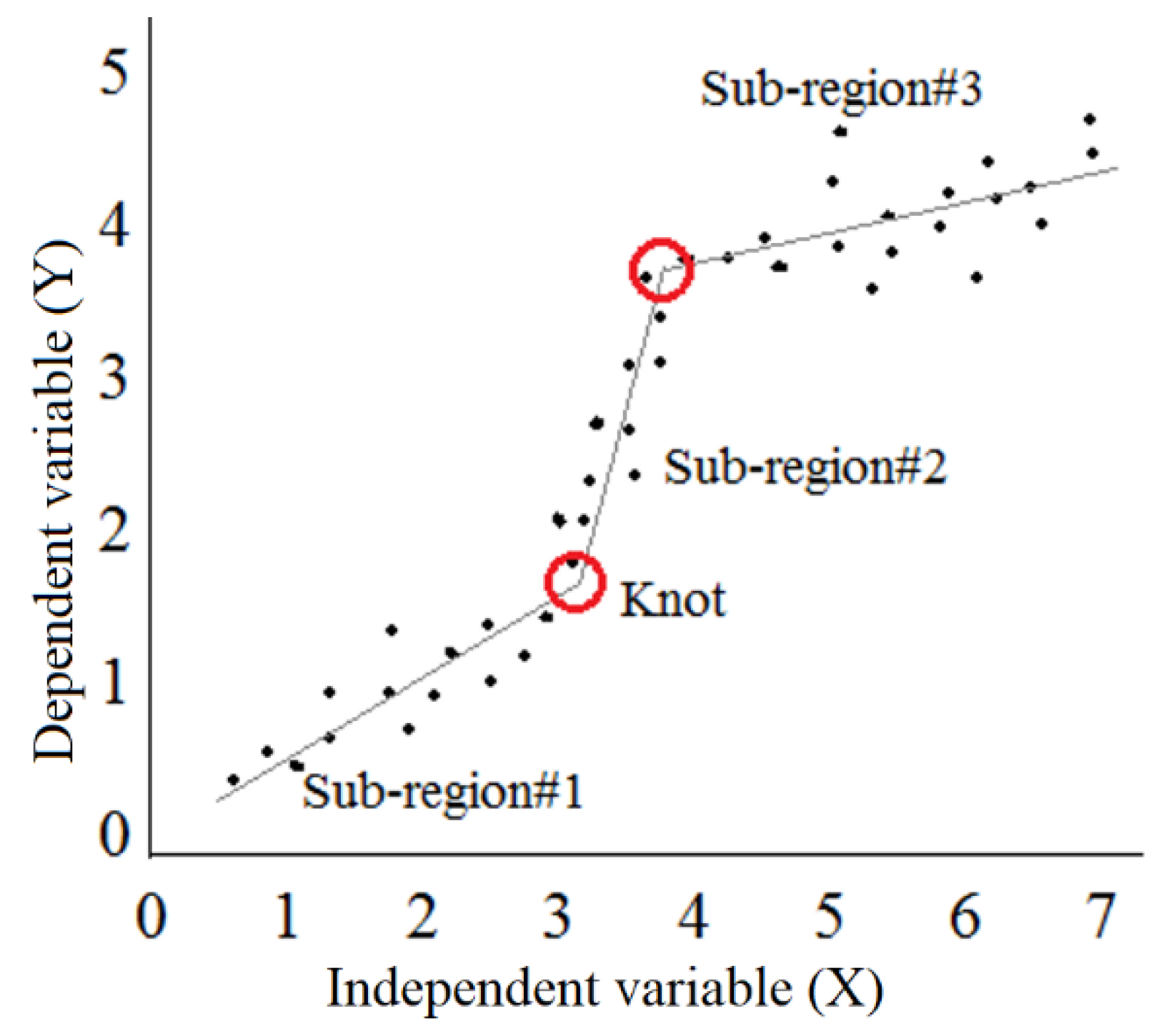
3.3. Multivariate Regression Spline (MARS)

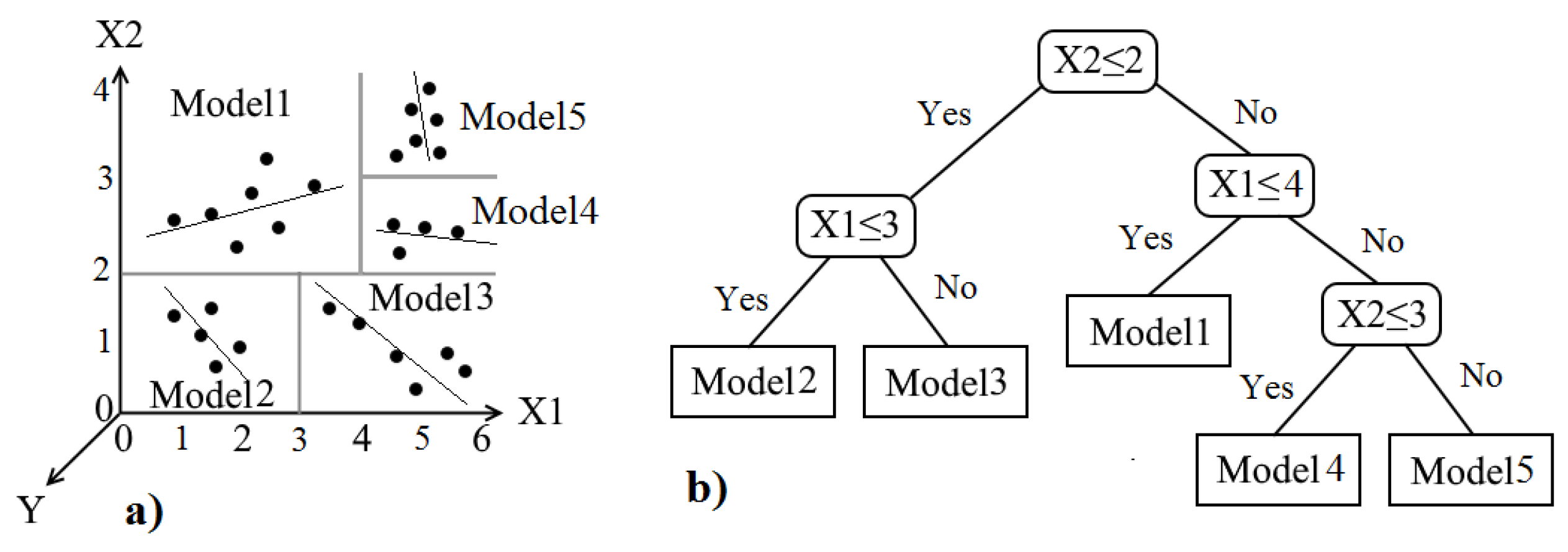
Proposed by Friedman in 1991 [47], multivariate adaptive regression spline is a procedure for fitting adaptive nonlinear functions using a piecewise nonparametric regression method. Unlike the black box models (e.g., ANNs), MARS models are deterministic, which means that in the final regression form the input variables are identified and the interactions between them are specified. Therefore, the MARS models are much easier to be interpreted than the other techniques [48,49,50]. Considering X as the only independent variable and Y as the dependent variable (target value), it can be seen in Figure 3 that the space of X variable is divided into three sub-regions with three different equations. These equations relate the independent variable space to the target of the system.

The endpoints of the segments of each sub-region are called knots (Figure 3). The resulting piecewise regression lines (basis functions, BFs) make the final regression form flexible and appropriate for capturing trends from linear functions as bellow [51]:

$$\widehat{Y}\left(\mathit{x}\right) ={\beta }_0+{\displaystyle \sum }_{i=1}^m{\beta }_i{BF}_i$$

(4)

where β_i = 0, 1, …, m are unknown coefficients and m is the number of basis functions (BF) which is determined using a piecewise linear function as follows [33]:

$$BFi= \left\{\max \left(0,\mathit{x}-C_i\right) , \max \left(0,C_i-\mathit{x}\right)\right\}$$

(5)

where C represents the knot which is a constant coefficient. By considering more independent variables, more equations will be added to the final regression form. In order to determine the location of knots, an adaptive regression algorithm is used. In addition, BFs are generated by a stepwise searching process. In brief, the main procedure of the MARS method is categorized into two parts of the forward and backward phases. The location of potential knots and BFs equations are specified in the forward phase. To modify and improve the modeling accuracy, unnecessary and the least effective variables are removed in the backward phase [48]. Further details for the mathematical procedure of the MARS method can be obtained from Friedman [47].

3.4. M5 Model Tree

Quinlan (1992) introduced a piecewise linear regression model, called the M5 model tree (M5Tree) [52,53], which has a tree structure based on binary decisions. The linear regression functions, which develop interconnection between the input and output vectors, can be extracted at the terminals (leaves) nodes.

Constructing an M5tree model requires two distinct phases; first the initial tree is generated and is then pruned. In the first phase, data sets are split into several subsets, which create a decision tree. In other words, the M5 model tree splits the data set space into subsets (sub-spaces) and generates a linear regression model [54,55]. As can be observed in Figure 4, the two-dimensional dynamic space of the input vector (X1 & X2) is split schematically into five subsets.

The splitting criterion is determined by assuming the standard deviation (sd) of the class values that reach a node. Based on the sd, the standard deviation reduction (SDR) can be calculated as the following relation [13,56]:

$$SDR=sd\left(T\right)-{\displaystyle \sum }_{ı=1}^n\frac{\left|T_i\right|}{\left|T\right|}sd\left(T_i\right)$$

(6)

where T stands for the set of examples that reaches the node, and T_i is the subset of examples with the ith outcome of the potential set. After the first phase (viz. constructing the initial tree), a huge tree-like structure might be generated, which may cause poor generalization. To cope with this problem, in the second phase, the overgrown tree is pruned.

3.5. Response Surface Methodology

The response surface methodology (RSM) presents the advantage of multiple regression analysis via a statistical technique to simulate a response space based on quantitative data obtained from the extracted multivariate equations as presented below [57]:

$$\widehat{Y}\left(\mathit{x}\right) ={\beta }_0+{\displaystyle \sum }_{i=1}^{\mathit{NV}}{\beta }_i{\mathit{x}}_i+{\displaystyle \sum }_{i=1}^{\mathit{NV}}{\displaystyle \sum }_{j=i}^{\mathit{NV}}{\beta }_{\mathit{ij}}{\mathit{x}}_i{\mathit{x}}_j$$

(7)

where NV denotes the number of input variables. β₀, β_i and β_ij are unknown coefficients for polynomial terms. During the mathematical process, RSM explores the influence of multiple independent variables on the response parameter and optimizes the trending procedure by tuning the number of required experiments [58,59,60,61].

3.6. Kriging Interpolation Approach

The kriging basis nonlinear model is a well-known interpolation approach to approximate geological problems [62]. It is defined by using stochastic terms according to the following relation [63,64]:

$$\widehat{Y}\left(\mathit{x}\right) =\widehat{\beta }f+r^T\left(X\right)R^{-1}\left(Y-\widehat{\beta }f\right)$$

(8)

where $\widehat{\beta }={\left[{\widehat{\beta }}_1,{\widehat{\beta }}_2,\dots ,{\widehat{\beta }}_m\right]}^T$ are regression coefficients for n-support points with m basic functions. The unknown coefficients are computed as follows [65]:

$$\widehat{\beta }={\left(f^T{R}^{-1}f\right)}^{-1}{f}^T{R}^{-1}Y$$

(9)

where $\widehat{Y}\left(X\right)$ is the predicted value. $R$ represents the correlation matrix which is given as:

$$R=\left[\begin{array}{ccc}\begin{array}{cc}\begin{array}{c}1\\ r\left(X_2,X_1\right)\end{array}& \begin{array}{c}r\left(X_1,X_2\right)\\ 1\end{array}\end{array}& \cdots & \begin{array}{c}r\left(X_1,X_n\right)\\ r\left(X_2,X_n\right)\end{array}\\ ⋮& \ddots & ⋮\\ \begin{array}{cc}r\left(X_n,X_1\right)& r\left(X_n,X_1\right)\end{array}& \cdots & 1\end{array}\right]$$

(10)

in which $r\left(X_i,X_j\right)$ is the cross-correlation function computed by the following relation:

$$r\left(X_i,X_j\right) =e^{\theta r_{ij}^2},r_{ij}= \parallel X_i-X_j\parallel$$

(11)

where, $r_{ij}$ is the distance between points, $X_i$ and $X_j$ and $\theta >0$ are unknown correlation parameters, which are determined as presented below [66,67,68,69]:

$$\theta =argMax(\frac{log[\mathit{det}R\left]+nlog\right[{\widehat{\sigma }}^2]}{2})$$

(12)

where n represents the number of training points, and ${\widehat{\sigma }}^2$ denotes the variance of the model obtained as:

$${\widehat{\sigma }}^2=\frac{{\left(Y-\widehat{\beta }f\right)}^T{R}^{-1}\left(Y-\widehat{\beta }f\right)}{n}$$

(13)

In the kriging model, the basis function $f$ can be defined as below:

$$f=\left[\begin{array}{ccc}\begin{array}{cc}\begin{array}{c}{f}_1\left(X_1\right)\\ f_1\left(X_2\right)\end{array}& \begin{array}{c}{f}_2\left(X_1\right)\\ f_2\left(X_2\right)\end{array}\end{array}& \cdots & \begin{array}{c}{f}_m\left(X_1\right)\\ f_m\left(X_2\right)\end{array}\\ ⋮& \ddots & ⋮\\ \begin{array}{cc}{f}_1\left(X_n\right)& f_2\left(X_n\right)\end{array}& \cdots & f_m\left(X_n\right)\end{array}\right]$$

(14)

where the vector [$f_1\left(X_1\right),f_2\left(X_1\right),\dots ,f_m\left(X_1\right)]$ includes the basic functions that are evaluated at the data input point of $X_1$, and m is the number of the basic functions. The basis function $f$ can be used as polynomial and exponential functions for original kriging and improved kriging, as presented in this study.

In the kriging models, the basic functions are considered as follows:

$$f\left(X_k\right) = \left\{1X_k\right\} where X =Mon,Ws,T_{max},T_{min},RH,SR,Hs$$

(15)

where $Mon$ represents the periodicity (month of the year), $Ws$ is wind speed (m/s), $T_{max}$ and $T_{min}$ are respectively the maximum and minimum temperature (°C), $RH$ is the relative humidity (%), $SR$ is the solar radiation (langley), and $Hs$ represents the hours of sunshine (h). The surrogate model that uses an adaptive kriging framework can be used for (i) reducing the computational burden and increase the accuracy results of the optimization problem [50,70], (ii) structural reliability analysis [65,68], and (iii) reliability-based design optimization [67,71].

3.7. Improved Kriging

In the fitness process of the kriging model, the basic function term, i.e., $\widehat{\beta }f$ is an important factor for providing a flexible prediction. The stochastic term, i.e., $r^T\left(X\right)R^{-1}(Y-\widehat{\beta }f)$, may produce a smaller covariance for approximating data with accurate basic function. Thus, the nonlinear form of the basic function can improve the accuracy of the EP predictions. A schematic comparative view of the exponential and linear polynomial functions is presented in Figure 5 to illustrate the fitness of the exponential basic function. We used the exponential basic function for the regression process instead of the linear basic function, in order to enhance the ability of the standard kriging model.

In improved kriging, the linear and exponential functions are used by the following basic function:

$$f\left(X_k\right) = \left\{1X_{k}exp\left(X_k\right)\right\}$$

(16)

where $X_k$ are the input variables and exp denotes the exponential operator. The prediction accuracy of the improved kriging model for the estimation of the EP is tested based on an untried data set using $r\left(X\right)$ in Equation (11) and predicted relation in Equation (8).

3.8. Methodology and Models Evaluation

The modeling process focuses on the monthly predictions of the EP based on two different scenarios, as presented below:

• Scenario I (without periodicity):

In the first scenario (#I), the monthly averaged of six meteorological parameters including wind speed (WS, m/s), relative humidity (RH, %), solar radiation (SR, Langley), sunshine hours (HS, h), minimum (Tmin, °C), and maximum temperatures (Tmax, °C), are considered as the input vectors of the applied models.

• Scenario II, (with periodicity):

In the second strategy, all of the mentioned independent meteorological parameters along with the time factor formed the input vector.

Due to the fact that in the second scenario, the order of the data is important for modeling, the time series cross-validation technique was applied. Thus, in both of the scenarios, 70% of the data was used for training the models, and the other 30% was used for the testing set. In the current work, the root mean square error (RMSE) was used as a measure of accuracy, while the mean bias error (MBE) was used as a measure of tendency. The absolute residual of the standard deviation between the actual EP values and the modeled ones (RSTD) was used as a measure of precision as presented below [60,72,73]:

$$RMSE=\sqrt{\frac{1}{N}{\displaystyle \sum }_{i=1}^N{({EPm}_i-{EPo}_i)}^2 }$$

(17)

$$MBE=\frac{1}{N}{\displaystyle {\displaystyle \sum }_{i=1}^N\left({EPm}_i-{EPo}_i^{}\right)}$$

(18)

$$R_{STD}=\left|{STD}_m-{STD}_O\right|$$

(19)

where N is the number of data, EPm_i represents the modeled EP for the ith data and EPo_i stands for the observed EP values for the ith data. In addition to the above-mentioned measures, other statistics and criteria such as the mean absolute error (MAE), mean absolute percentage error (MAPE), Willmott index (d), total pan evaporation (Tot-EP), maximum value of the relative error between the calculated and observed EP (MAX (RE)) were also used for the evaluation of the applied methods [58].

$$MAE=\frac{{\displaystyle {\displaystyle \sum }_{i=1}^N}\left|{EPm}_i-{EPo}_i\right|}{N}$$

(20)

$$MAPE=\frac{1}{N}{\displaystyle {\displaystyle \sum }_{i=1}^N\frac{\left|{EPm}_i-{EPo}_i^{}\right|}{{EPo}_i^{}}}$$

(21)

$$d=1-\frac{{\displaystyle {\displaystyle \sum }_{i=1}^N(EP{m}_i-EP{o}_i^{}}{)}^2}{{\displaystyle {\displaystyle \sum }_{i=1}^N(\left|EP{m}_i-EPmean\right|+\left|EP{m}_i^{}-EPmean\right|}{)}^2}$$

(22)

where EPmean is the mean of monthly EP. In this study, the Wilcoxon nonparametric statistical hypothesis test is also implemented to evaluate the performance of statistical versus soft computing models at the 95% confidence level. The maximum relative absolute error ((Max (RE)) was computed as max (RE_i) and RE_i = ($|{\widehat{Y}}_i-Y_i)|/Y_i$, where ${\widehat{Y}}_i$ an $Y_i$ indicate the estimated and observed pan evaporation.

4. Comparison and Results

4.1. Evaluation of the Applied Models

Table 1. Comparing the results of the applied models without periodicity (Scenario #1) for Adana station in the testing period.

Category	Model	MAE (mm)	RMSE (mm)	MBE (mm)	d	Max (RE)	Mean * (mm)	STD * (mm)	Tot-EP * (mm)	MAPE
Statistical	kriging	0.712	0.891	0.228	0.958	86.31	4.36	2.19	501.63	0.213
	Improved kriging	0.659	0.843	0.172	0.964	72.89	4.31	2.26	495.13	0.184
	RSM	0.736	0.933	0.142	0.956	79.08	4.28	2.29	491.71	0.205
Soft computing models	MARS	0.701	0.855	0.221	0.962	87.78	4.35	2.23	500.78	0.203
	M5Tree	0.704	0.890	0.197	0.960	80.77	4.33	2.29	498.11	0.190
	SVR	0.668	0.828	0.223	0.964	135.32	4.36	2.15	501.08	0.208
	ANN(LM)	0.685	0.861	0.197	0.962	83.32	4.33	2.25	498.01	0.195
	ANN(CG)	0.739	0.930	0.157	0.955	66.74	4.29	2.22	493.49	0.207
	RBFNN	0.712	0.892	0.229	0.958	86.31	4.36	2.19	501.68	0.213

* The mean, standard deviation (STD) and total pan evaporation (Tot-EP) of the actual data points are mean = 4.134 mm, STD = 2.256 mm and Tot-EP = 475.4 mm, respectively. Optimal structure of SVR: (C = 10, ε = 0.5, σ = 85), ANN (LM): 6-7-1, ANN (CG): 6-8-1, RBFNN: 6-40-1 (σ = 2).

and

Table 2. Comparing the results of the applied models with periodicity (Scenario #2) for Adana station in the testing period.

Category	Structures	MAE (mm)	RMSE (mm)	MBE (mm)	d	Max (RE)	Mean * (mm)	STD * (mm)	Tot-EP * (mm)	MAPE
Statistical	kriging	0.730	0.912	0.224	0.957	88.79	4.36	2.20	501.11	0.220
	Improved kriging	0.646	0.821	0.168	0.966	76.97	4.30	2.26	494.75	0.181
	RSM	0.768	0.972	0.138	0.953	100.96	4.27	2.31	491.22	0.210
Soft computing models	MARS	0.697	0.859	0.146	0.962	63.13	4.28	2.24	492.19	0.193
	M5Tree	0.715	0.897	0.192	0.959	80.77	4.33	2.28	497.45	0.197
	SVR	0.648	0.796	0.173	0.966	106.42	4.31	2.12	495.30	0.200
	MLP-LM	0.746	0.949	0.206	0.954	99.85	4.34	2.26	499.06	0.205
	MLP-CG	0.764	0.976	0.189	0.952	71.22	4.32	2.29	497.16	0.208
	RBNN	0.682	0.842	0.233	0.963	85.82	4.37	2.21	502.21	0.214

* The mean, standard deviation (STD) and total pan evaporation (Tot-EP) of the actual test data points are mean = 4.134 mm, STD = 2.256 mm and Tot-EP = 475.4 mm, respectively. Optimal structure of SVR: (C = 5, ε = 0.3, σ = 80), ANN (LM): 7-14-1, ANN (CG): 7-12-1, RBFNN: 7-35-1 (σ = 5).

report the comparison statistics of the applied data-driven models for the Adana station for the first and second scenarios. For the first scenario (without periodicity), the improved kriging model has the lowest MAE (0.659 mm), MAPE (0.189), RMSE (0.843 mm) and the highest d (0.964), followed by the SVR model. Based on the MAE, d, and RMSE values, the ANN-CG and RSM models provided the weakest results. However, the M5Tree model gave the worst Max (RE) value (135.32). The mean and total pan evaporations were also better approximated by the improved kriging compared to the other models. In the second scenario, the improved kriging model presented a better value of MAE than the SVR model (improved kriging = 0.646 mm vs. SVR = 0.648 mm), but worse values for RMSE (improved kriging = 0.821 mm vs. SVR = 0.796 mm) and could not be seen as the being better than the SVR model.

In general, all of the applied statistical and soft computing models approximated the EP values satisfactory (with d > 0.95 and RMSE < 1 mm). In

Table 3. The general performance of the applied models in terms of accuracy, precision, and tendency for Adana Station in the testing period.

	Scenario I, without Periodicity					Scenario II, with Periodicity
Category	Model	Accuracy	Precision	Tendency	Best Model(s)	Accuracy	Precision	Tendency	Best Model(s)
Statistical	Kriging	M	L	+		M	L	+
	Improved kriging	H	H	+	*	H	H	+	*
	RSM	L	M	+		L	L	+
Soft computing models	MARS	H	H	+	*	M	H	+
	M5Tree	M	M	+		M	M	+
	SVR	H	L	+		H	L	+
	MLP-LM	M	H	+		L	H	+
	MLP-CG	L	M	+		L	M	+
	RBNN	L	L	+		H	M	+

Note: Accuracy is based on RMSE (mm), precision is based on RSTD, and tendency is based on MBE. Accuracy and precision: H: high (3 best values), M: moderate (3 median values), L: low (3 worst values); Tendency: +: Over-predicted (positive values); N: neutral (absolute value < 0.01 mm). Best models have been chosen based on acted best at least in two of the three criteria.

, the best predictive model is presented as the improved kriging model based on attaining two of the highest position of the three elements of accuracy, precision, and tendency.

Figure 6 demonstrates the observed and estimated EP values of the applied models for the two scenarios, the Adana Station, (a) without periodicity, and (b) with periodicity. It is clear from the fit line equations and R² values that the improved kriging model has less distributed properties than the other models for both cases.

The comparison statistics of the applied models are given in

Table 4. Comparison of statistical errors for the applied models without periodicity (scenario #1) for Antakya Station in the testing period.

Category	Model	MAE (mm)	RMSE (mm)	MBE (mm)	d	Max (RE)	Mean * (mm)	STD * (mm)	Tot-EP * (mm)	MAPE
Statistical	kriging	0.555	0.717	−0.190	0.974	56.81	4.34	2.17	399.39	0.142
	Improved kriging	0.489	0.626	−0.001	0.981	48.06	4.53	2.35	416.77	0.119
	RSM	0.540	0.687	−0.132	0.978	60.99	4.40	2.36	404.77	0.129
Soft computing models	MARS	0.510	0.637	0.107	0.981	60.01	4.64	2.32	426.71	0.130
	M5Tree	0.722	0.998	−0.234	0.949	58.18	4.30	2.22	395.33	0.158
	SVR	0.463	0.613	−0.012	0.981	54.12	4.52	2.18	415.77	0.115
	MLP-LM	0.528	0.681	0.099	0.976	105.46	4.63	2.20	426.01	0.145
	MLP-CG	0.525	0.651	0.100	0.980	49.28	4.63	2.36	426.11	0.126
	RBFNN	0.476	0.610	−0.035	0.983	47.64	4.50	2.39	413.67	0.117

* The mean, standard deviation (STD) and total pan evaporation (Tot-EP) of the actual test data points are mean= 4.532 mm, STD = 2.295 mm and Tot-EP = 416.9 mm, respectively. Optimal structure of SVR: (C = 1600, ε = 0.25, σ = 80), ANN(LM): 6-9-1, ANN(CG): 6-7-1, RBFNN: 6-30-1 (σ = 15).

and

Table 5. Comparison of statistical errors for the applied models with periodicity (scenario #2) for Antakya Station in the testing period.

Category	Model	MAE (mm)	RMSE (mm)	MBE (mm)	d	Max (RE)	Mean * (mm)	STD * (mm)	Tot-EP * (mm)	MAPE
Statistical	kriging	0.560	0.721	−0.188	0.973	62.26	4.55	2.35	418.14	0.145
	Improved kriging	0.471	0.601	0.014	0.983	43.68	4.42	2.34	407.02	0.114
	RSM	0.579	0.701	−0.107	0.976	67.19	4.42	2.15	406.53	0.155
Soft computing models	MARS	0.517	0.638	0.094	0.980	48.89	4.32	2.26	397.37	0.132
	M5Tree	0.677	0.970	−0.212	0.953	49.04	4.34	2.17	399.62	0.142
	SVR	0.496	0.664	−0.113	0.977	49.49	4.53	2.24	416.47	0.117
	MLP-LM	0.492	0.625	−0.005	0.981	44.51	4.63	2.26	425.98	0.118
	MLP-CG	0.508	0.623	0.099	0.981	68.50	4.45	2.12	409.60	0.132
	RBFNN	0.483	0.632	−0.079	0.979	48.67	4.32	2.26	397.37	0.122

* The mean, standard deviation (STD) and total pan evaporation (Tot-EP) of the actual test data points are mean= 4.532 mm, STD = 2.295 mm and Tot-EP = 416.9 mm, respectively. Optimal structure of SVR: (C = 600, ε = 0.3, σ = 80), ANN (LM): 7-12-1, ANN (CG): 7-14-1, RBFNN: 7-30-1 (σ = 15).

for the Antakya Station. In the first scenario, the improved kriging model outperformed the other statistical models considering all of the given measures in Table 4. Nonetheless, in comparison to the SVR—as the best soft computing model—the improved kriging model provided the best performance for the MBE (−0.001) value, it failed in sustaining its superiority over the SVR for the MAE (improved kriging = 0.489 mm vs. SVR = 0.463 mm) and RMSE (improved kriging = 0.626 mm vs. SVR = 0.613 mm) criteria.

For the second scenario (Table 5), the improved kriging surpassed all the other applied statistical and soft computing models considering MAE, MAPE, RMSE, and d. In this scenario, the MLP-LM was the best soft computing model in predicting the EP values based on the MAE, MBE, d, and Max (RE) values.

Table 6. The general performance of the applied predictive models in terms of accuracy, precision, and tendency for Antakya Station in the testing period.

		Scenario I, without Periodicity				Scenario II, with Periodicity
Category	Model	Accuracy	Precision	Tendency	Best Model(s)	Accuracy	Precision	Tendency	Best Model(s)
Statistical	Kriging	L	H	−		L	L	−
	Improved kriging	H	H	N	*	H	M	+	*
	RSM	L	L	−		L	M	−
Soft computing models	MARS	M	H	+		M	H	+
	M5Tree	L	M	−		L	L	−
	SVR	H	L	−		M	M	−
	MLP-LM	M	M	+		H	H	N	*
	MLP-CG	M	M	+		H	H	+	*
	RBNN	H	L	−		M	L	−

Note: Accuracy is based on RMSE (mm), precision is based on RSTD, and tendency is based on MBE. Accuracy and precision: H: high (3 best values), M: moderate (3 median values), L: low (3 worst values); Tendency: −: under-predicted (negative values); +: over-predicted (positive values); N: neutral (absolute value < 0.01 mm). Best models have been chosen based on attaining at least two of the three accuracies (=H), precision (=H), and tendency (=N) criteria.

presents the best predictive models in terms of three perspectives of accuracy, precision, and tendency. As expected, the improved kriging performed better than the other models in the first scenario (without periodicity), while the MLP-LM and MLP-CG were also among the best models for the second scenario (with periodicity).

Figure 7 presents the observed and estimated values of the EP of the Antakya station of applied models a) without periodicity and b) with periodicity. From Figure 7, it is clear that the improved kriging, MARS, and MLP-CG models have similar graphs and they have less scattered predations than the other two models for the two modeling scenarios. It can also be seen that the M5Tree has the most scattered predicted values.

The ratio of the Willmott index of agreement (d) to the MAE can be used as a measure to compare the accuracy of different models. This statistic (d/MAE) varies from 0 to ∞. The larger value of the d/MAE denotes the better calibration of the applied model (Keshtegar et al., 2018). The calculated d/MAE ratios of the applied models are illustrated in Figure 8 for both stations. In general, it is apparent that the improved kriging has higher accuracy than the other models. It can also be observed that better results were given by the improved kriging model considering the periodicity (scenario II). Figure 8 shows that the SVR is the second-best accurate model in predicting EP values, which is similar to the results in Table 3 and Table 6 (marked with “H”). Despite being the most accurate soft computing model, the SVR did not act well on the precision and tendency of the predicted values, and as a result, it was not specified as the best model in Table 3 and Table 6.

4.2. Hypothesis Testing

The results of the significance test of the predicted values of statistical techniques and soft computing models using the Mann–Whitney test are presented in

Table 7. p-Values of the Mann–Whitney Test for statistical methods versus soft computing models in Adana Station.

		Soft Computing Models
		M5Tree	RBNN	MLP-LM	MLP-CG	SVR	MARS
Statistical models	RSM	0.792	0.899	0.865	0.654	0.970	0.720
	Kriging	0.878	0.844	0.984	0.964	0.970	0.977
	Improved kriging	0.988	0.724	0.870	0.918	0.886	0.895

and

Table 8. p-Values of the Mann–Whitney Test for statistical methods versus soft computing models in Antakya Station.

		Soft Computing Models
		M5Tree	RBNN	MLP-LM	MLP-CG	SVR	MARS
Statistical models	RSM	0.824	0.873	0.626	0.631	0.786	0.638
	kriging	0.904	0.722	0.478	0.532	0.648	0.518
	Improved kriging	0.709	0.997	0.757	0.785	0.910	0.778

for the Adana and Antakya Stations, respectively. In the Mann–Whitney test, the null and alternative hypotheses are as follows (η is the median):

The null hypothesis, H0: η1 − η2 = 0.

The alternative hypothesis, H1: η1 − η2 ≠ 0.

The results of Table 7 and Table 8 clearly reveal that there is no significant difference between the performance of the statistical models (RSM, kriging, and improved kriging) and soft computing models (M5Tree, RBNN, MLP-LM, MLP-CG, and MARS) at 95% and 99% confidence levels, as they have p-values greater than 0.05 and 0.01. In other words, the Mann–Whitney nonparametric test implies that the null hypothesis was not rejected, and none of the applied statistical-based predictive models surpasses the other soft computing models at the 0.05 and 0.01 levels of significance.

5. Discussion

This paper aimed to challenge the performance of different statistical and soft computing models based on (i) mathematical (accuracy, precision, and tendency), and (ii) statistical (at the 0.01 and 0.05 levels of significance) perspectives. In accordance with the mathematical comparisons (Table 1, Table 2, Table 4 and Table 5, and Figure 8), it was concluded that the improved kriging model performed better than the other applied models, which means that an improved statistical model might even be able to surpass soft computing models.

Figure 9 illustrates the Taylor diagrams for (a) Adana and (b) Antakya Stations. As shown by these figures, the kriging models provide a better prediction for agreement than the RSM but worse than the soft computing models (viz. SVR, MARS, and RBFNN). The SVR provides a superior correlation with the observed data compared to the other soft computing models. As can be seen in Figure 9, the improved kriging enhanced the predictions of the standard kriging model.

There is no doubt that in most cases, soft computing models perform better than traditional statistical models. Similarly, the standard kriging and RSM models failed to surpass the soft computing models due to linear cross-correlation regressed function based on the statistical measures. This assessment is based on pertinent studies in the literature. For instance, in a comparative study between the capability of machine learning versus ANN, and statistical technique versus MLR, for EP prediction, it was found that the model efficiency and correlation coefficient of the ANN was higher than the MLR model for the calibration and validation phases [20]. The same result has been noted for the superiority of ANFIS model over the MLR statistical model [74]. However, it is worth noting that the majority of recent published studies have solely focused on the evaluation of several machine learning models [11,32]. Investigating the outcomes of these studies indicates that the machine learning models perform well in predicting evaporation at different climatical regions.

In this study, in addition to the mathematical evaluation of the potential performance of statistical and soft computing models, the results of the Mann–Whitney hypothesis test were also taken into account. The outcomes of the Mann–Whitney hypothesis test showed that none of the soft computing applied models has significant superiority over the statistical ones. In other words, despite their ability to model nonlinear phenomena, soft computing models should not be taken into granted as the preliminary predictive models. The improved versions of the RSM or kriging-based statistical techniques can improve the accuracy of the prediction of nonlinear problems. Thus, the improved statistical kriging technique uses the exponential transformation of input variables and can also be applied for other engineering problems with nonlinear complex relations. Furthermore, the competency of this method can be apprised by comparing it with machine learning models for complex problems with highly nonlinear relations.

6. Conclusions

The soft computing models and statistical techniques are useful frameworks for making predictions of complex climatological indices, such as the hydrological pan evaporation (EP). The improved kriging method was presented as a statistical technique for the accurate prediction of the EP. The RSM, kriging, and improved kriging models were compared with soft computing models, such as the SVR, M5tree, MARS, RBNN, MLP-LM, and MLP-CG. Two different input scenarios, namely with and without periodicity, were applied for the modeling process in the Antakya and the Adana stations located in Turkey. The abilities of statistical models versus soft computing schemes were compared with several statistical measures. The key findings of the study are summarized below:

• Soft computing using machine learning models such as the SVR, MARS, MLP-ML, and RBNN provided more accurate predictions than the M5Tree and RSM.
• The kriging model, as well as the SVR, RBFNN and MLP-ML, provided better performances compared to the RSM and M5Tree.
• It was found that the developed improved kriging model performed better than the other applied models, including the soft computing (SVR, RBNN, MLP-ML, and MARS) and standard statistical (kriging and RSM) models.
• By comparing the performances of the improved kriging method with six other applied models, it can be concluded that the proposed kriging framework can be successfully applied for this current hydrological challenge while its performances for other hydrological stations and other complex, sophisticated problems should be discussed in future.

References

1. Kişi, Ö. Daily pan evaporation modelling using a neuro-fuzzy computing technique. J. Hydrol. 2006, 329, 636–646. [Google Scholar] [CrossRef]
2. Li, D.; Pan, M.; Cong, Z.; Zhang, L.; Wood, E. Vegetation control on water and energy balance within the budyko framework. Water Resour. Res. 2013, 49, 969–976. [Google Scholar] [CrossRef]
3. Yan, D.; Lai, Z.; Ji, G. Using budyko-type equations for separating the impacts of climate and vegetation change on runoff in the source area of the yellow river. Water 2020, 12, 3418. [Google Scholar] [CrossRef]
4. Almorox, J.; Grieser, J. Calibration of the hargreaves–samani method for the calculation of reference evapotranspiration in different köppen climate classes. Hydrol. Res. 2016, 47, 521–531. [Google Scholar] [CrossRef] [Green Version]
5. Srivastava, A.; Sahoo, B.; Raghuwanshi, N.S.; Chatterjee, C. Modelling the dynamics of evapotranspiration using variable infiltration capacity model and regionally calibrated hargreaves approach. Irrig. Sci. 2018, 36, 289–300. [Google Scholar] [CrossRef]
6. Srivastava, A.; Sahoo, B.; Raghuwanshi, N.S.; Singh, R. Evaluation of variable-infiltration capacity model and modis-terra satellite-derived grid-scale evapotranspiration estimates in a river basin with tropical monsoon-type climatology. J. Irrig. Drain. Eng. 2017, 143, 04017028. [Google Scholar] [CrossRef] [Green Version]
7. Kisi, O.; Zounemat-Kermani, M. Comparison of two different adaptive neuro-fuzzy inference systems in modelling daily reference evapotranspiration. Water Resour. Manag. 2014, 28, 2655–2675. [Google Scholar] [CrossRef]
8. Dong, L.; Zeng, W.; Wu, L.; Lei, G.; Chen, H.; Srivastava, A.K.; Gaiser, T. Estimating the pan evaporation in northwest china by coupling catboost with bat algorithm. Water 2021, 13, 256. [Google Scholar] [CrossRef]
9. Majhi, B.; Naidu, D. Pan evaporation modeling in different agroclimatic zones using functional link artificial neural network. Inf. Process. Agric. 2021, 8, 134–147. [Google Scholar] [CrossRef]
10. Duan, Z.; Bastiaanssen, W. Evaluation of three energy balance-based evaporation models for estimating monthly evaporation for five lakes using derived heat storage changes from a hysteresis model. Environ. Res. Lett. 2017, 12, 024005. [Google Scholar] [CrossRef] [Green Version]
11. Wang, S.; Fu, Z.-Y.; Chen, H.-S.; Nie, Y.-P.; Wang, K.-L. Modeling daily reference et in the karst area of northwest Guangxi (China) using gene expression programming (gep) and artificial neural network (ann). Theor. Appl. Climatol. 2016, 126, 493–504. [Google Scholar] [CrossRef]
12. Sudheer, K.; Gosain, A.; Mohana Rangan, D.; Saheb, S. Modelling evaporation using an artificial neural network algorithm. Hydrol. Process. 2002, 16, 3189–3202. [Google Scholar] [CrossRef]
13. Kisi, O. Pan evaporation modeling using least square support vector machine, multivariate adaptive regression splines and m5 model tree. J. Hydrol. 2015, 528, 312–320. [Google Scholar] [CrossRef]
14. Keskin, M.E.; Terzi, Ö. Artificial neural network models of daily pan evaporation. J. Hydrol. Eng. 2006, 11, 65–70. [Google Scholar] [CrossRef]
15. Moghaddamnia, A.; Gousheh, M.G.; Piri, J.; Amin, S.; Han, D. Evaporation estimation using artificial neural networks and adaptive neuro-fuzzy inference system techniques. Adv. Water Resour. 2009, 32, 88–97. [Google Scholar] [CrossRef]
16. Kim, S.; Shiri, J.; Kisi, O. Pan evaporation modeling using neural computing approach for different climatic zones. Water Resour. Manag. 2012, 26, 3231–3249. [Google Scholar] [CrossRef]
17. Gao, B.; Xu, X. Derivation of an exponential complementary function with physical constraints for land surface evaporation estimation. J. Hydrol. 2021, 593, 125623. [Google Scholar] [CrossRef]
18. Wang, H.; Yan, H.; Zeng, W.; Lei, G.; Ao, C.; Zha, Y. A novel nonlinear arps decline model with salp swarm algorithm for predicting pan evaporation in the arid and semi-arid regions of china. J. Hydrol. 2020, 582, 124545. [Google Scholar] [CrossRef]
19. Wu, L.; Huang, G.; Fan, J.; Ma, X.; Zhou, H.; Zeng, W. Hybrid extreme learning machine with meta-heuristic algorithms for monthly pan evaporation prediction. Comput. Electron. Agric. 2020, 168, 105115. [Google Scholar] [CrossRef]
20. Singh, A.; Singh, R.; Kumar, A.S.; Kumar, A.; Hanwat, S.; Tripathi, V. Evaluation of soft computing and regression-based techniques for the estimation of evaporation. J. Water Clim. Chang. 2021, 12, 32–43. [Google Scholar] [CrossRef]
21. Tabari, H.; Marofi, S.; Sabziparvar, A.-A. Estimation of daily pan evaporation using artificial neural network and multivariate non-linear regression. Irrig. Sci. 2010, 28, 399–406. [Google Scholar] [CrossRef]
22. Kisi, O.; Genc, O.; Dinc, S.; Zounemat-Kermani, M. Daily pan evaporation modeling using chi-squared automatic interaction detector, neural networks, classification and regression tree. Comput. Electron. Agric. 2016, 122, 112–117. [Google Scholar] [CrossRef]
23. Tezel, G.; Buyukyildiz, M. Monthly evaporation forecasting using artificial neural networks and support vector machines. Theor. Appl. Climatol. 2016, 124, 69–80. [Google Scholar] [CrossRef]
24. Keshtegar, B.; Kisi, O. Modified response-surface method: New approach for modeling pan evaporation. J. Hydrol. Eng. 2017, 22, 04017045. [Google Scholar] [CrossRef]
25. Wang, L.; Niu, Z.; Kisi, O.; Yu, D. Pan evaporation modeling using four different heuristic approaches. Comput. Electron. Agric. 2017, 140, 203–213. [Google Scholar] [CrossRef]
26. Wang, L.; Kisi, O.; Hu, B.; Bilal, M.; Zounemat-Kermani, M.; Li, H. Evaporation modelling using different machine learning techniques. Int. J. Climatol. 2017, 37, 1076–1092. [Google Scholar] [CrossRef]
27. Ghorbani, M.; Deo, R.C.; Yaseen, Z.M.; Kashani, M.H.; Mohammadi, B. Pan evaporation prediction using a hybrid multilayer perceptron-firefly algorithm (mlp-ffa) model: Case study in north iran. Theor. Appl. Climatol. 2018, 133, 1119–1131. [Google Scholar] [CrossRef]
28. Majhi, B.; Naidu, D.; Mishra, A.P.; Satapathy, S.C. Improved prediction of daily pan evaporation using deep-lstm model. Neural Comput. Appl. 2020, 32, 7823–7838. [Google Scholar] [CrossRef]
29. Sebbar, A.; Heddam, S.; Djemili, L. Predicting daily pan evaporation (e pan) from dam reservoirs in the mediterranean regions of algeria: Opelm vs oselm. Environ. Process. 2019, 6, 309–319. [Google Scholar] [CrossRef]
30. Al-Mukhtar, M. Modeling the monthly pan evaporation rates using artificial intelligence methods: A case study in iraq. Environ. Earth Sci. 2021, 80, 1–14. [Google Scholar] [CrossRef]
31. Mohamadi, S.; Ehteram, M.; El-Shafie, A. Accuracy enhancement for monthly evaporation predicting model utilizing evolutionary machine learning methods. Int. J. Environ. Sci. Technol. 2020, 17, 3373–3396. [Google Scholar] [CrossRef]
32. Yaseen, Z.M.; Al-Juboori, A.M.; Beyaztas, U.; Al-Ansari, N.; Chau, K.-W.; Qi, C.; Ali, M.; Salih, S.Q.; Shahid, S. Prediction of evaporation in arid and semi-arid regions: A comparative study using different machine learning models. Eng. Appl. Comput. Fluid Mech. 2020, 14, 70–89. [Google Scholar] [CrossRef] [Green Version]
33. Keshtegar, B.; Mert, C.; Kisi, O. Comparison of four heuristic regression techniques in solar radiation modeling: Kriging method vs rsm, mars and m5 model tree. Renew. Sustain. Energy Rev. 2018, 81, 330–341. [Google Scholar] [CrossRef]
34. Heddam, S.; Keshtegar, B.; Kisi, O. Predicting total dissolved gas concentration on a daily scale using kriging interpolation, response surface method and artificial neural network: Case study of columbia river basin dams, USA. Nat. Resour. Res. 2020, 29, 1801–1818. [Google Scholar] [CrossRef]
35. Gupta, A.K. Predictive modelling of turning operations using response surface methodology, artificial neural networks and support vector regression. Int. J. Prod. Res. 2010, 48, 763–778. [Google Scholar] [CrossRef]
36. Ladlani, I.; Houichi, L.; Djemili, L.; Heddam, S.; Belouz, K. Estimation of daily reference evapotranspiration (et 0) in the north of algeria using adaptive neuro-fuzzy inference system (anfis) and multiple linear regression (mlr) models: A comparative study. Arab. J. Sci. Eng. 2014, 39, 5959–5969. [Google Scholar] [CrossRef]
37. Zounemat-Kermani, M.; Mahdavi-Meymand, A. Hybrid meta-heuristics artificial intelligence models in simulating discharge passing the piano key weirs. J. Hydrol. 2019, 569, 12–21. [Google Scholar] [CrossRef]
38. Hasanipanah, M.; Keshtegar, B.; Thai, D.-K.; Troung, N.-T. An ann-adaptive dynamical harmony search algorithm to approximate the flyrock resulting from blasting. Eng. Comput. 2020, 1–13. [Google Scholar] [CrossRef]
39. Johansson, E.M.; Dowla, F.U.; Goodman, D.M. Backpropagation learning for multilayer feed-forward neural networks using the conjugate gradient method. Int. J. Neural Syst. 1991, 2, 291–301. [Google Scholar] [CrossRef]
40. Yu, Q.; Hou, Z.; Bu, X.; Yu, Q. Rbfnn-based data-driven predictive iterative learning control for nonaffine nonlinear systems. IEEE Trans. Neural Netw. Learn. Syst. 2019, 31, 1170–1182. [Google Scholar] [CrossRef]
41. Esfe, M.H. Designing an artificial neural network using radial basis function (rbf-ann) to model thermal conductivity of ethylene glycol–water-based tio 2 nanofluids. J. Therm. Anal. Calorim. 2017, 127, 2125–2131. [Google Scholar] [CrossRef]
42. Santamaría-Bonfil, G.; Reyes-Ballesteros, A.; Gershenson, C. Wind speed forecasting for wind farms: A method based on support vector regression. Renew. Energy 2016, 85, 790–809. [Google Scholar] [CrossRef]
43. Zhang, J.; Xiao, M.; Gao, L.; Chu, S. Probability and interval hybrid reliability analysis based on adaptive local approximation of projection outlines using support vector machine. Comput. Aided Civ. Infrastruct. Eng. 2019, 34, 991–1009. [Google Scholar] [CrossRef]
44. Zhang, J.; Xiao, M.; Gao, L.; Chu, S. A combined projection-outline-based active learning kriging and adaptive importance sampling method for hybrid reliability analysis with small failure probabilities. Comput. Methods Appl. Mech. Eng. 2019, 344, 13–33. [Google Scholar] [CrossRef]
45. Chiogna, G.; Marcolini, G.; Liu, W.; Ciria, T.P.; Tuo, Y. Coupling hydrological modeling and support vector regression to model hydropeaking in alpine catchments. Sci. Total Environ. 2018, 633, 220–229. [Google Scholar] [CrossRef]
46. Chen, J.-L.; Yang, H.; Lv, M.-Q.; Xiao, Z.-L.; Wu, S.J. Estimation of monthly pan evaporation using support vector machine in three gorges reservoir area, china. Theor. Appl. Climatol. 2019, 138, 1095–1107. [Google Scholar] [CrossRef]
47. Friedman, J.H. Multivariate adaptive regression splines. Ann. Stat. 1991, 19, 1–67. [Google Scholar] [CrossRef]
48. Jalali-Heravi, M.; Asadollahi-Baboli, M.; Mani-Varnosfaderani, A. Shuffling multivariate adaptive regression splines and adaptive neuro-fuzzy inference system as tools for qsar study of sars inhibitors. J. Pharm. Biomed. Anal. 2009, 50, 853–860. [Google Scholar] [CrossRef]
49. Zhang, J.; Gao, L.; Xiao, M. A new hybrid reliability-based design optimization method under random and interval uncertainties. Int. J. Numer. Methods Eng. 2020, 121, 4435–4457. [Google Scholar] [CrossRef]
50. Zhang, Y.; Gao, L.; Xiao, M. Maximizing natural frequencies of inhomogeneous cellular structures by kriging-assisted multiscale topology optimization. Comput. Struct. 2020, 230, 106197. [Google Scholar] [CrossRef]
51. Zhang, W.; Goh, A.T. Evaluating seismic liquefaction potential using multivariate adaptive regression splines and logistic regression. Geomech. Eng. 2016, 10, 269–284. [Google Scholar] [CrossRef]
52. Keshtegar, B.; Kisi, O. Rm5tree: Radial basis m5 model tree for accurate structural reliability analysis. Reliab. Eng. System Saf. 2018, 180, 49–61. [Google Scholar] [CrossRef]
53. Kisi, O.; Keshtegar, B.; Zounemat-Kermani, M.; Heddam, S.; Trung, N.-T. Modeling reference evapotranspiration using a novel regression-based method: Radial basis m5 model tree. Theor. Appl. Climatol. 2021, 145, 639–659. [Google Scholar] [CrossRef]
54. Pal, M.; Deswal, S. M5 model tree based modelling of reference evapotranspiration. Hydrol. Process. Int. J. 2009, 23, 1437–1443. [Google Scholar] [CrossRef]
55. Sattari, M.T.; Pal, M.; Apaydin, H.; Ozturk, F. M5 model tree application in daily river flow forecasting in sohu stream, turkey. Water Resour. 2013, 40, 233–242. [Google Scholar] [CrossRef]
56. Seghier, M.E.A.B.; Keshtegar, B.; Correia, J.A.; Lesiuk, G.; De Jesus, A.M. Reliability analysis based on hybrid algorithm of m5 model tree and monte carlo simulation for corroded pipelines: Case of study x60 steel grade pipes. Eng. Fail. Anal. 2019, 97, 793–803. [Google Scholar] [CrossRef]
57. Kowsar, R.; Keshtegar, B.; Miyamoto, A. Understanding the hidden relations between pro-and anti-inflammatory cytokine genes in bovine oviduct epithelium using a multilayer response surface method. Sci. Rep. 2019, 9, 1–17. [Google Scholar] [CrossRef] [PubMed] [Green Version]
58. Keshtegar, B.; Seghier, M.e.A.B. Modified response surface method basis harmony search to predict the burst pressure of corroded pipelines. Eng. Fail. Anal. 2018, 89, 177–199. [Google Scholar] [CrossRef]
59. Bezerra, M.A.; Santelli, R.E.; Oliveira, E.P.; Villar, L.S.; Escaleira, L.A. Response surface methodology (rsm) as a tool for optimization in analytical chemistry. Talanta 2008, 76, 965–977. [Google Scholar] [CrossRef]
60. Keshtegar, B.; Gholampour, A.; Thai, D.-K.; Taylan, O.; Trung, N.-T. Hybrid regression and machine learning model for predicting ultimate condition of frp-confined concrete. Compos. Struct. 2021, 262, 113644. [Google Scholar] [CrossRef]
61. Keshtegar, B.; Bagheri, M.; Fei, C.-W.; Lu, C.; Taylan, O.; Thai, D.-K. Multi-extremum-modified response basis model for nonlinear response prediction of dynamic turbine blisk. Eng. Comput. 2021, 1–12. [Google Scholar] [CrossRef]
62. Lucy, L.B. A numerical approach to testing the fission hypothesis. Astron. J. 1977, 82, 1013–1024. [Google Scholar] [CrossRef]
63. Gao, L.; Xiao, M.; Shao, X.; Jiang, P.; Nie, L.; Qiu, H. Analysis of gene expression programming for approximation in engineering design. Struct. Multidiscip. Optim. 2012, 46, 399–413. [Google Scholar] [CrossRef]
64. Keshtegar, B.; Heddam, S.; Sebbar, A.; Zhu, S.-P.; Trung, N.-T. Svr-rsm: A hybrid heuristic method for modeling monthly pan evaporation. Environ. Sci. Pollut. Res. 2019, 26, 35807–35826. [Google Scholar] [CrossRef] [PubMed]
65. Fei, C.-W.; Lu, C.; Liem, R.P. Decomposed-coordinated surrogate modeling strategy for compound function approximation in a turbine-blisk reliability evaluation. Aerosp. Sci. Technol. 2019, 95, 105466. [Google Scholar] [CrossRef]
66. Echard, B.; Gayton, N.; Lemaire, M. Ak-mcs: An active learning reliability method combining kriging and monte carlo simulation. Struct. Saf. 2011, 33, 145–154. [Google Scholar] [CrossRef]
67. Xiao, M.; Zhang, J.; Gao, L. A system active learning kriging method for system reliability-based design optimization with a multiple response model. Reliab. Eng. Syst. Saf. 2020, 199, 106935. [Google Scholar] [CrossRef]
68. Xiao, M.; Zhang, J.; Gao, L.; Lee, S.; Eshghi, A.T. An efficient kriging-based subset simulation method for hybrid reliability analysis under random and interval variables with small failure probability. Struct. Multidiscip. Optim. 2019, 59, 2077–2092. [Google Scholar] [CrossRef]
69. Zhu, S.-P.; Keshtegar, B.; Tian, K.; Trung, N.-T. Optimization of load-carrying hierarchical stiffened shells: Comparative survey and applications of six hybrid heuristic models. Arch. Comput. Methods Eng. 2021, 28, 4153–4166. [Google Scholar] [CrossRef]
70. Lu, C.; Feng, Y.-W.; Fei, C.-W.; Bu, S.-Q. Improved decomposed-coordinated kriging modeling strategy for dynamic probabilistic analysis of multicomponent structures. IEEE Trans. Reliab. 2019, 69, 440–457. [Google Scholar] [CrossRef]
71. Keshtegar, B.; Hao, P. A hybrid descent mean value for accurate and efficient performance measure approach of reliability-based design optimization. Comput. Methods Appl. Mech. Eng. 2018, 336, 237–259. [Google Scholar] [CrossRef]
72. Keshtegar, B.; Nehdi, M.L.; Kolahchi, R.; Trung, N.-T.; Bagheri, M. Novel hybrid machine leaning model for predicting shear strength of reinforced concrete shear walls. Eng. Comput. 2021, 1–12. [Google Scholar] [CrossRef]
73. El Amine Ben Seghier, M.; Keshtegar, B.; Tee, K.F.; Zayed, T.; Abbassi, R.; Trung, N.T. Prediction of maximum pitting corrosion depth in oil and gas pipelines. Eng. Fail. Anal. 2020, 112, 104505. [Google Scholar] [CrossRef]
74. Malik, A.; Kumar, A. Pan evaporation simulation based on daily meteorological data using soft computing techniques and multiple linear regression. Water Resour. Manag. 2015, 29, 1859–1872. [Google Scholar] [CrossRef]
Figure 1. The studied stations in the Mediterranean region of Turkey; Adana and Antakya.
Water 13 02451 g001
Figure 2. Box-plots of independent variables and EP for (a) Adana (b) Antakya Stations.
Water 13 02451 g002
Figure 3. A schematic sketch for the illustration of sub-regions of the MARS method.
Water 13 02451 g003
Figure 4. Basic sketch for the M5 tree model; (a) splitting the input vector into subsets, (b) M5 tree structure.
Water 13 02451 g004
Figure 5. Schematic view of basic function using linear and exponential forms for data of (a) maximum temperature and (b) hours of sunshine.
Water 13 02451 g005
Figure 6. The observed and estimated EP (a) without and (b) with periodicity for Adana station in the testing period.
Water 13 02451 g006
Figure 7. The observed and estimated EP (a) without and (b) with periodicity for Antakya Station in the testing period.
Water 13 02451 g007
Figure 8. Bar charts showing the d/MAE ratio for the applied models in the testing period for Adana and Antakya Stations.
Water 13 02451 g008
Figure 9. Taylor diagram for different models in the testing phase of (a) Adana station (b) Antakya station.
Water 13 02451 g009