Estimating Organic and Inorganic Part of Suspended Solids from Sentinel 2 in Different Inland Waters

Abstract

Inland waters are very sensitive ecosystems that are mainly affected by pressures and impacts within their watersheds. One of water’s dominant constituents is the suspended particulate matter that affects the optical properties of water bodies and can be detected from remote sensors. It is important to know their composition since the ecological role they play in water bodies depends on whether they are mostly organic compounds (phytoplankton, decomposition of plant matter, etc.) or inorganic compounds (silt, clay, etc.). Nowadays, the European Space Agency Sentinel-2 mission has outstanding characteristics for measuring inland waters’ biophysical variables. This work developed algorithms that can estimate the total concentration of suspended matter (TSM), differentiating organic from inorganic fractions, through the combined use of Sentinel-2 images with an extensive database obtained from reservoirs, lakes and marshes within eastern zones of the Iberian Peninsula. For this, information from 121 georeferenced samples collected throughout 40 field campaigns over a 4-year period was used. All possible two-band combinations were obtained and correlated with the biophysical variables by fitting linear regression between the field data and bands combination. The results determined that only using bands 705 or 783 lead to the obtaining the amount of total suspended matter and their organic and inorganic fractions, with errors of 10.3%, 14.8% and 12.2%, respectively. Therefore, remote sensing provides information about total suspended matter dynamics and characteristics as well as its spatial and temporal variation, which would help to study its causes.

1. Introduction

Lentic inland water (lakes, reservoirs and wetlands) are very sensitive ecosystems to pressures and impacts on their watershed, which also affect their climate system [1]. In the Mediterranean Basin, climate models predict an increase in the intensity of floods and the severity of droughts in the coming decades [2], bringing on more frequent episodes of torrential rains which may accelerate the silting processes in addition to increasing amount of organic matter and suspended solids. These changes can also alter the functions of aquatic ecosystems and compromise their uses [3]. Thus, the quality improvement and protection of these waters have become a global priority of the 21st century making it necessary to know, at every moment, the quality of these water bodies for ecological and management purposes. Water quality is a general descriptor of water properties in terms of physical, chemical, thermal, and/or biological characteristics. By combining in situ measurements and collecting water samples that are subsequently analyzed in a laboratory, we can provide accurate information for a specific place in time and space. However, from a spatial or temporal point of view, these sampling campaigns do not provide enough information needed for an accurate assessment or management of the entire water body. As a complement, remote sensing observations facilitates the knowledge of these measures and, especially, their spatial variation [4] in near real time which makes them a cost-effective way of monitoring water quality [5].

Passive remote sensing is the process of inferring surface parameters from measurements of the electromagnetic radiation coming from the water’s surface. This radiation can be a reflection of solar energy or energy emitted from the Earth, which is in the thermal infrared (TIR) and microwave portions of the spectrum. The reflected solar light in the visible and near infrared spectrum is used in hydrology for water quality studies [4]. Copernicus is a joint initiative of the European Commission (EC) and the European Space Agency (ESA), designed to establish a European capacity to provide and use monitoring information from an environment and security point of view, through different satellite missions known under the name of Sentinel. Copernicus mission was initially optimized for vegetation studies, urban planning and terrestrial ecosystems. However, the inclusion of new bands in the red-edge (the limit of red and infrared spectral regions), as well as its radiometric quality and high spatial resolution, have proven its usefulness for inland waters studies [6]. Data provided by the Copernicus mission increases the usefulness of limnological data collected in situ [7], thanks to the synoptic view and frequent satellite passes (temporal resolution of 5 days). These characteristics make this sensor an exceptional device for measuring inland waters’ biophysical variables [5].

The presence of different suspended particles in surface water can significantly change the backscattering properties of water bodies. Remote sensing methods for monitoring water quality rely upon the capacity to measure these changes in the backscattered spectral signature of water in order to report these measured changes by empirical or analytical models as water quality variables [4]. Variables often derived quantitatively using remote sensing methods include phytoplankton pigments such as chlorophyll-a [Chl-a] [8], cyanobacterial pigment phycocyanin (PC) [9], concentration of total suspended matter (TSM) [10], absorption by colored dissolved organic matter (CDOM) [11], Secchi disk depth (SDD) or water transparency [12], turbidity [13] and water temperature [7]. It is also viable to establish the contour and surface of water bodies [14].

This work is centered on the TSM, the name provided to the total mass of suspended particles measured per volume of water [15] held in the water of a stream, river, lake or reservoir by turbulence [16]. TSM is, in general, a mixture of live and detritic (non-living) particulate organic matter, such as phytoplankton or detritus, and inorganic matter such as clay, silt and other suspended minerals [17,18]. High TSM values (usually >1000 mg/L) affects the depth at which the photosynthetically active radiation can arrive at The physical alterations they produce can, simultaneously, lead to undesirable aesthetic effects [19], increase water treatment costs [20], reduce navigability of canals and decrease the longevity of dams and reservoirs [21]. In addition, in the abundant presence of suspended solids with high organic content, decomposition can occur in situ and reduce the dissolved oxygen levels in water, producing a critical oxygen shortage [20]. If sediments are smaller than <63 µm in diameter, it is possible for toxic or harmful substances to adhere to them, which in turn, facilitates their transport [22]. Hence its importance as a variable, which is one of the most commonly used for the characterization of water and participates in the water quality indices that currently exist [23]. The ecological consequences that TSM can produce depend on whether they are composed mostly of organic compounds (phytoplankton or its detritus, decomposition of plant matter, etc.) or inorganic compounds (sand, silt, clay, etc.). Estimation of its concentration is possible using multispectral remote sensing tools. Most water quality studies by remote sensing focus solely on the determination of TSM concentration, and only a few authors separate the estimation of organic and inorganic solids, as for example the recent studies carried out by Kratzer et al. [24], Schartau et al. [25] and Kutser et al. [26].

The main objective of this study is to develop algorithms that can estimate the total concentration of suspended solids, differentiating the organic from the inorganic fraction, through the combined use of Sentinel-2 images and an extensive database of different types of water bodies in Spain.

2. Materials and Methods

2.1. Study Area

In this work, databases of different projects were used, obtained in the Iberian Peninsula during field campaigns from July 2016 to November 2020 sampling 28 reservoirs in the Ebro watershed, eight reservoirs in the Júcar watershed, as well as 17 marshes surrounding the Albufera of Valencia lagoon. We focused our study on reservoirs with different trophic status, from oligotrophic to eutrophic or hypertrophic (as in the case of Albufera lagoon and marshes).

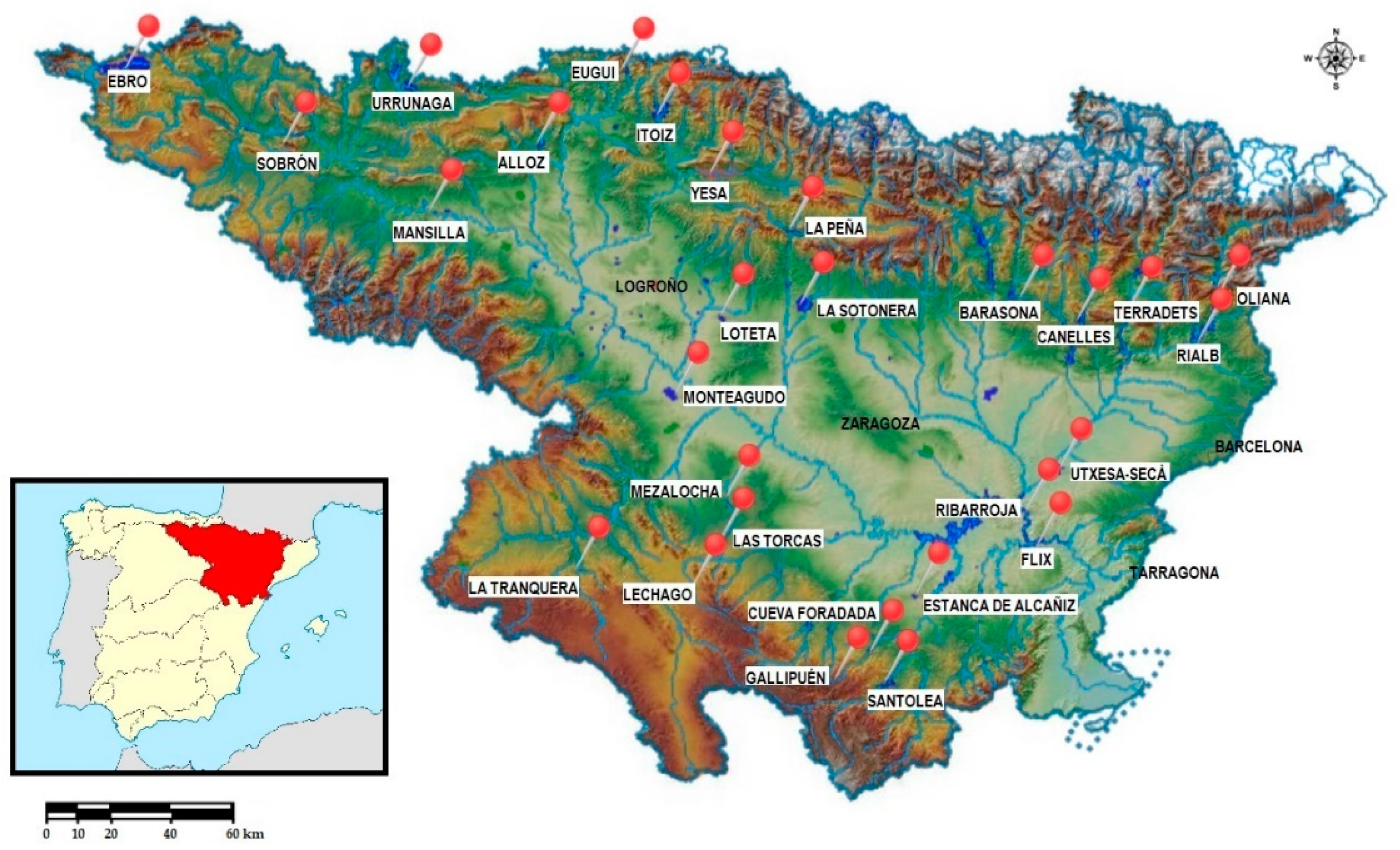
2.1.1. Ebro Hydrographic Watershed

The Ebro River watershed is the largest hydrographic basin in Spain, with a total area that occupies 17% of the national territory [27]. The Ebro River, which is the main Spanish river, drains 85,530 km² along the southern-facing slopes of the Cantabrian and Pyrenees Mountain ranges, as well as the Northeastern-facing slopes of the Iberian Massif, outflowing into the Mediterranean Sea at Amposta, 180 km south of Barcelona [28,29]. In the Ebro River watershed, there are currently about 200 water bodies with artificial or modified natural-river characteristics (reservoirs, dammed lakes, weirs, artificial lakes and ponds) that present a great diversity in size, capacity, uses and landscape context. These hydraulic works range from small, low-volume dams to large reservoirs of thousands hm³ of capacity [30], the largest reservoirs being Mequinenza, Canelles, Ebro and Yesa. The reservoirs in this watershed vary from 1530 hm³ of capacity and 75.4 km² of maximum surface to 2.5 hm³ of capacity and 4.25 km² of surface [27].

Apart from supplying irrigation, many socio-economic activities in this basin need water for their development: population, industry, livestock, hydroelectricity, refrigeration, aquaculture, and other recreational uses, such as navigation [29,30]. This work was carried out over the summer, when we analyzed 28 reservoirs (Figure 1), collecting a single sample between June and August, which was the time of maximum stability of the water mass due to stratification, and the most adverse period for water quality [31].

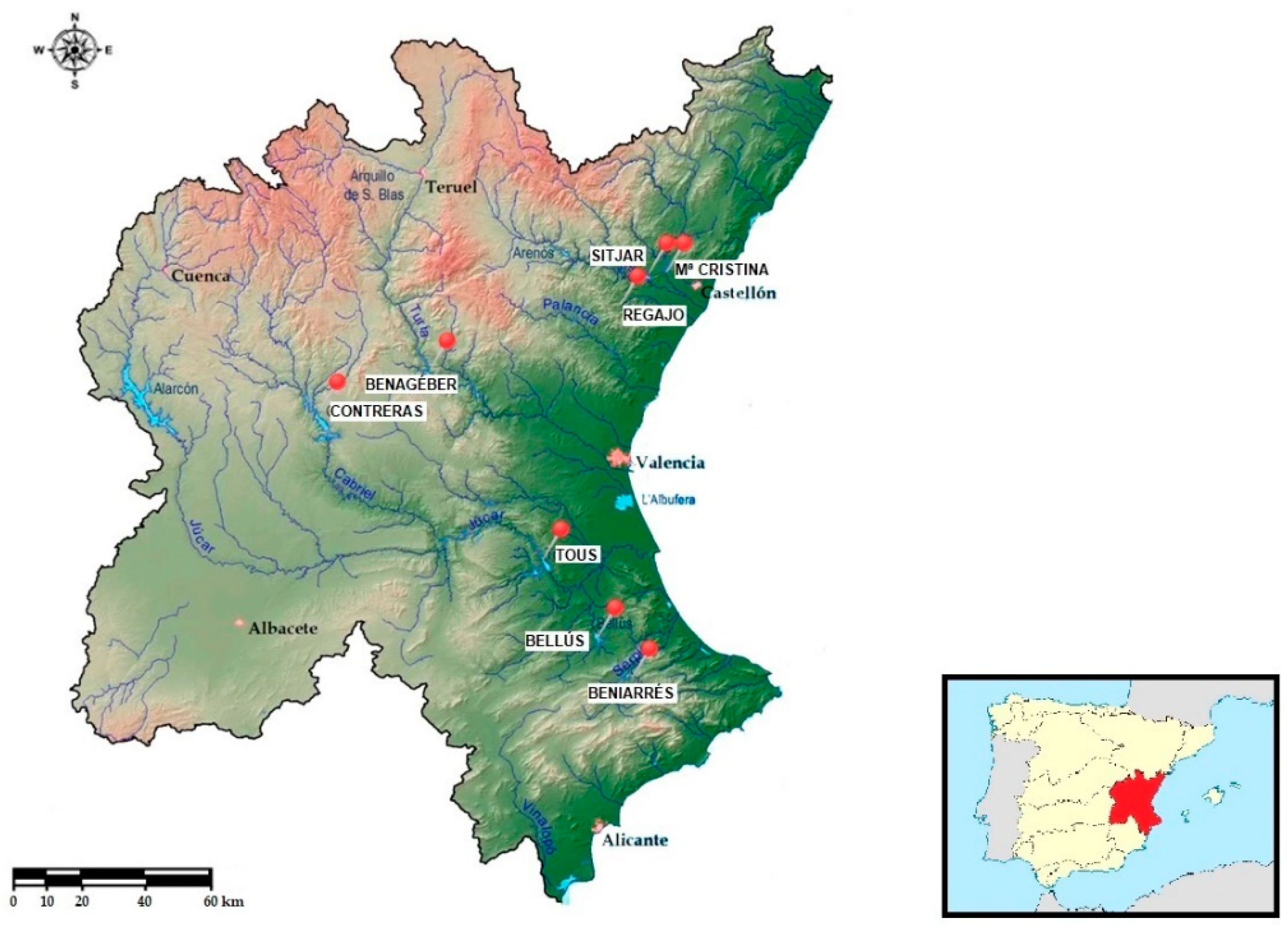
2.1.2. Júcar Hydrographic Watershed

The Júcar River watershed is located in the eastern part of the Iberian Peninsula and occupies an area of 42,989 km². Its formed by the aggregation of watersheds that flow into the Mediterranean Sea [32], its main rivers being the Júcar, Turia, Mijares, Palancia, Serpis and Vinalopó [33]. It is a highly-regulated watershed, with 27 reservoirs and a total capacity of 2646 hm³ [34] the largest reservoirs are Alarcón, Tous, Contreras and Benagéber. The reservoirs in this basin vary from 1112 hm³ capacity and 68.4 km² maximum surface to 6 hm³ capacity and 0.82 km² surface [32].

Water is used mainly for irrigation, urban and industry water supply and hydropower generation [35]. A total of eight reservoirs were selected to carry out this study, and samples were collected during June and August (Figure 2).

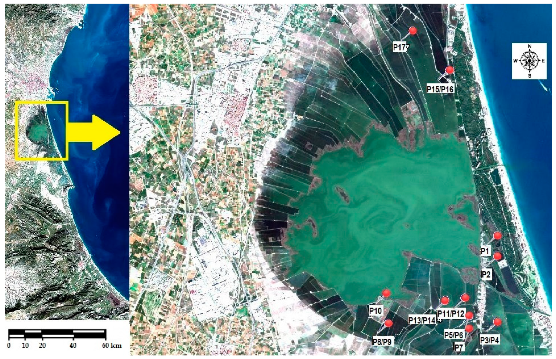
2.1.3. Albufera Marshes

On the alluvial platform of Júcar and Turia Rivers lies the Albufera of Valencia Natural Park, one of the most important wetlands of Spain (300 km²), which has a lagoon with an approximate area of 27 km² [37]. This natural reserve includes the lake and the surrounding areas composed of large extensions of marshes and several rows of dunes, a first line of mobile dunes, along with others, fixed by a pine and scrub forest, that protect the wetland from the coast [38]. The marshes that surround the Albufera are modified and mainly occupied by rice crops. These rice fields function as a temporary wetland with a hydrological cycle of medium summer flooding during rice growth, emptying in September for harvesting, and high flood (maximum) during autumn and winter, drying again in spring for farming work until sowing of a new crop cycle in April–May. If during January–February the flooded fields are drained again, their water drains through the lake [39]. Once the rice has been harvested the residual straw is organized into bales, which usually are stacked near the rice fields, with the possibility of strong weather conditions returning this to the flooded rice field. Considering that the water has poor circulation, the residual straw results in decomposing organic matter that will produce anoxic or hypoxic conditions in the water, along with mineralization. Their presence may also produce interferences in the satellite reflectance.

During the autumn season, specifically in November, a total of 17 points in the marshes were sampled to carry out this study (Figure 3).

2.2. Field Data Collection and Laboratory Measurements

In all remote sensing studies, synchronous with satellite images, field data are needed. These in situ measurements provide the possibility to calibrate and validate the local or regional retrieval algorithms [40]. From July 2016 to November 2020, a total of 40 field campaigns were completed, and 121 georeferenced samples were collected. Following sampling protocols [41], at the reservoirs we located, by echo-sounding, a point in the area of maximum depth, which has to be situated 300–500 m from the dam to prevent disturbances by the possible outflow. These protocols were not applied to the samplings in the marshes due to the fact that they are shallow areas (0.5 m), therefore the sampling was carried out at a point 10–15 m from the shore. For each reservoir and marsh, between 1 and 4 in situ spectrometric measuring points were taken at a suitable distance from shoreline to avoid mixed pixels (land-water mixed reflectance).

Table A1. Summary of sampled water bodies. Abbreviations: lat.: latitude; lon.: longitude.

Name	Position (Decimal Degree)		Watershed	Volume (hm3)	Samples	Season
	Lat.	Lon.
Alloz	42.71	−1.95	Ebro	65.31	1	Summer
Barasona	42.13	0.32	Ebro	85	1	Summer
Bellús	38.39	−0.47	Júcar	69	7	Summer
Benagéber	39.72	−1.09	Júcar	221	13	Summer
Beniarrés	38.80	−0.35	Júcar	27	3	Summer
Canelles	42.03	0.65	Ebro	678	2	Summer
Contreras	39.62	−1.53	Júcar	361	13	Summer
Cueva Foradada	40.98	−0.69	Ebro	22.08	2	Summer
Ebro	42.97	−4.07	Ebro	540	1	Summer
Estanca de Alcañiz	41.06	−0.18	Ebro	7	1	Summer
Eugui	42.97	−1.51	Ebro	21.88	1	Summer
Flix	41.23	0.54	Ebro	11.41	1	Summer
Gallipuén	40.87	−0.41	Ebro	4.36	1	Summer
Itoiz	42.8	−1.36	Ebro	417.47	1	Summer
La Casota de Baldoví	39.3	−0.32	Albufera	<0.1	2	Autumn
La Loteta	41.8	−1.32	Ebro	104.85	1	Summer
La Peña	42.3	−0.73	Ebro	15.45	1	Summer
La Sotonera	42.1	−0.69	Ebro	189	5	Summer
La Tranquera	41.2	−1.79	Ebro	84.26	3	Summer
Las Torcas	41.2	−1.08	Ebro	6.66	1	Summer
Lechago	40.9	−1.29	Ebro	18.6	1	Summer
Mª Cristina	40.02	−0.16	Júcar	18	4	Summer
Mansilla	42.1	−2.93	Ebro	67.7	2	Summer
Mezalocha	41.4	−1.07	Ebro	3.92	2	Summer
Monteagudo	41.3	−2.17	Ebro	10	1	Summer
Oliana	42.1	1.29	Ebro	101.1	3	Summer
Regajo	39.89	−0.52	Júcar	6	7	Summer
Rialb	41.9	1.20	Ebro	402.8	2	Summer
Ribarroja	41.2	0.43	Ebro	209.6	2	Summer
Santolea	40.7	−0.32	Ebro	60	1	Summer
Séquia Vella Palmar	39.3	−0.31	Albufera	<0.1	2	Autumn
Sequiol de Romero	39.	−0.33	Albufera	<0.1	2	Autumn
Sitjar	40.01	−0.23	Júcar	49	6	Summer
Sobrón	42.7	−3.10	Ebro	20	2	Summer
Tancat de L’Illa	39.3	−0.31	Albufera	<0.1	1	Autumn
Tancat de L’Olla	32.3	−0.31	Albufera	<0.1	1	Autumn
Tancat del Fangar	39.3	−0.32	Albufera	<0.1	3	Autumn
Tancat de Mília	39.3	−0.35	Albufera	<0.1	1	Autumn
Tancat de Sacarés	39.3	−0.35	Albufera	<0.1	2	Autumn
Tancat de la Taüt	39.3	−0.33	Albufera	<0.1	2	Autumn
Terradets	42.05	0.88	Ebro	33.19	1	Summer
Tous	39.13	−0.65	Júcar	379	8	Summer
Turbina Rabisanxo	39.3	−0.35	Albufera	<0.1	1	Autumn
Urrúnaga	42.9	−2.65	Ebro	72	1	Summer
Utxesa-Secà	41.4	0.51	Ebro	4	1	Summer
Yesa	42.6	−1.17	Ebro	447	1	Summer
Total					121

and

Table A2. Samples collected by year and place.

Watershed/Year	2016	2017	2018	2019	2020
Júcar	2	30	29	0	0
Ebro	9	11	15	7	0
Albufera Marshes	0	0	0	0	17

in Appendix A shows the number of samples for each test site, their location and additional information.

Secchi disk is a standard white disc 20 cm in diameter that is submerged vertically until it is no longer visible. Secchi disk depth (SDD) consists of measuring the mean value of the point at which the disk completely disappears and the depth at which it reappears [42]. SDD was measured in situ. At each sampling point, water samples were collected and stored in refrigeration at 4 °C in the dark, for later transport to the laboratory. PVC tubes were used to take samples from the surface down to SDD, because integrated samples are more representatives. [Chl-a] was measured by fluorometry (Turner C3) and in the laboratory by spectrometry. Samples were filtered through 0.4–0.6 µm pore size Whatman GF/F glass fiber filters, extracted according to Shoaf & Lium [43] and calculated as in Jeffrey & Humphrey [44]. TSM was determined by gravimetry [45], consecutively measuring the particulate matter retained on individual filters Whatman 934–AH type (1.5 µm pore). This method involves two steps; first, the filter that contains the particulate matter is dried at 105 °C to obtain the value of dry TSM and, subsequently, it is heated at 460 °C for six hours. The value obtained is from the particulate inorganic matter (PIM) and, by difference from the value obtained previously (TSM), particulate organic matter (POM) is calculated. The combustion of particulate organic matter (POM) supposes a loss of weight that we usually call Loss on Ignition (LOI).

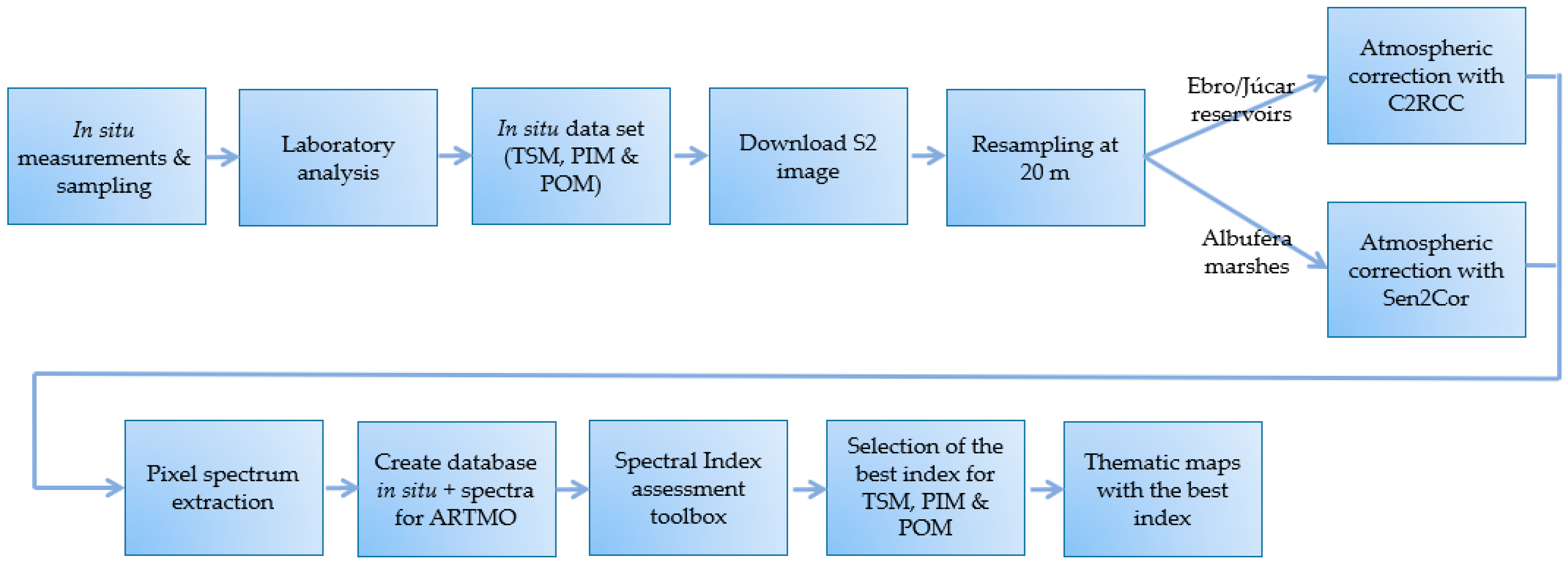
2.3. Satellite Images and Atmospheric Correction

The ESA Sentinel-2 mission (S2) consists of a two-satellite constellation flying in tandem: S2A (launch date: 23 June 2015) and S2B (launch date: 7 March 2017). Each satellite is equipped with the MSI sensor (Multispectral Instrument), which measures Earth’s reflected radiance for 13 spectral bands, from visible to near infrared (NIR) and short-wave infrared (SWIR), with spatial resolutions of 10, 20 and 60 m [46].

Table 1. Main characteristics of S2-MSI spectral bands [46].

Band Number	Central Wavelength (nm)	Bandwidth (nm)	Spatial Resolution (m)
1	443	20	60
2	490	65	10
3	560	35	10
4	665	30	10
5	705	15	20
6	740	15	20
7	783	20	20
8	842	115	10
8a	865	20	20
9	945	20	60
10	1380	30	60
11	1610	90	20
12	2190	180	20

summarizes the principal features of S2-MSI.

The field campaigns were planned on cloud-free days in which the S2 satellites acquired images over the selected areas [5,47]. The time gap between the satellite image capture and the field collection campaigns was extended for at least three days, one before and one after the day of image capture, following the methodology of Kutser [48]. Images used in this study were downloaded from Copernicus web (European Union) and USGS (United States Geological Survey) archives. The dataset consists of S2-Level 1C imagery (the level 1C (top of atmosphere; TOA) images are georeferenced without atmospheric correction) for both the Ebro and Júcar reservoirs and S2-Level 2A (bottom of atmosphere; BOA) imagery. The level 2A images are georeferenced with atmospheric correction that gives reflectance below the atmosphere for the water bodies and marshes, according to [6]. The images from the Sentinel satellites have the possibility of being processed with a program that was specially developed by ESA for them, the SNAP (Sentinel Application Platform, Brockman Consulting), which is free to download and use.

The retrieval of water constituents, or its optical properties, is achieved from the water leaving reflectance spectrum, measured at the top of atmosphere and thus requiring a correction for atmospheric effects. This multivariate problem is extremely challenging in optically complex water (or Case-2 waters). The C2RCC (Case-2 Regional CoastColour), a processor built-in SNAP, is composed of a set of additional neural networks that are trained to perform the inversion of spectrum for the atmospheric correction. Those neural networks are also capable of performing the retrieval of inherent optical properties of the water body [49]. A version developed for turbid water, called C2RCC for Complex Waters (known as C2X), is also available at SNAP. Sen2Cor is a Level 2A (L2A) processor whose main purpose is to correct single-date Sentinel-2 Level-1C products from the effects of the atmosphere in order to deliver a Level-2A surface reflectance product [50]. Sen2Cor processor was designed for vegetation and land, but also provides good results for eutrophic or hypertrophic waters, such as Albufera of Valencia and its surrounding marshes [6,51]. All images were resampled at 20 m, those corresponding to the Júcar and Ebro reservoirs were corrected using the C2RCC processors according to their trophic status, while those corresponding to the Albufera’s marshes were discharged with the atmospheric correction given by the Sen2Cor processor. If the water bodies studied vary in their trophic status between oligotrophic and hypereutrophic, then the most appropriate atmospheric corrector must be chosen. To obtain reflectance data, nine pixels’ parameter values were extracted around the coordinates of each measurement point; subsequently, the mean of these 9 values is calculated and the outliers are eliminated using the standard deviation and the mean of the remaining values’ results as the spectrum of the measured parameter [52]. With these spectrums, and together with the field data, the database for the spectral indices calibration was built.

2.4. Automatic Water Quality Products from C2RCC Processor

The C2RCC processor automatically generates, by default, two band folders with the products corresponding to the IOPs (inherent optical properties of water) and the concentrations of chlorophyll and total suspended solids. These last two products are calculated through arithmetic conversion factors from the IOPs [51]. However, this is not the case with the Sen2Cor processor, because it is a generic atmospheric correction method, not developed specifically for water. Therefore, only automatic water quality products for the Ebro and Júcar reservoirs could be obtained by means of C2RCC.

2.5. Algorithm Retrieval

An atmospherically corrected multispectral image contains reflectance data in different bands centered at certain wavelengths. An idea of the bands to be used can be obtained from the spectrum of the element under study, which will provide its absorption and reflectivity characteristics. These bands can be used, by themselves, or combined by some arithmetic operation, to obtain a correlation between the field data and the data from the satellite sensor [52,53].

With the Spectral Index (SI) assessment toolbox in the Automated Radiative Transfer Models Operator (ARTMO) package [54], all possible band combinations of different formulations can be defined and evaluated. This tool allows the transformation of spectral observations into useful estimates. The basic principle is to correlate mathematical combinations of reflectance measured at different wavelength ranges, with biophysical variables of interest. Simple ratio (SR = R1/R2) and normalized difference (ND: (R2 − R1)/(R2 + R1)) formulations as well as various curve fitting functions (linear, exponential, power, logarithmic, and polynomial) have been used to obtain all two-band reflectance (Ri) combinations according to these formulations. Implementing a cross validation (CV) tool, a portion of the database was used to train the model while another portion was used to validate, and then all combinations were calculated. Thus, ARTMO selects the best index, calibrating and validating all data. ARTMO provides the results and their correlation matrix ordered according to their average value of determination coefficient R². All infrared simple bands have also been correlated with the biophysical variables of interest (Figure 4).

The process for the setting-up of the algorithms was developed using all data of TSM, POM and PIM. Once we had three data sets, algorithms were calibrated with a regression between the field data, and band combinations using S2-MSI spectral bands, finding the best fitting function. Then, the algorithms were validated adjusting a linear regression between field and estimated data, using as goodness, the determination coefficient (R²), the root mean-square error (RMSE) and the normalized root-mean-square error (NRMSE).

$$RMSE=\sqrt{\frac{{{\displaystyle \sum }}_{i=1}^N{\left(x_i^{estimated}-x_i^{measured}\right)}^2}{N}}$$

(1)

$$NRMSE=\frac{RMSE}{\sigma \left(Y\right)}$$

(2)

where x_i^estimated is the predicted value, χ_i^measured is the observed value, N is the sample size and σ(Y) is the highest predicted value.

3. Results

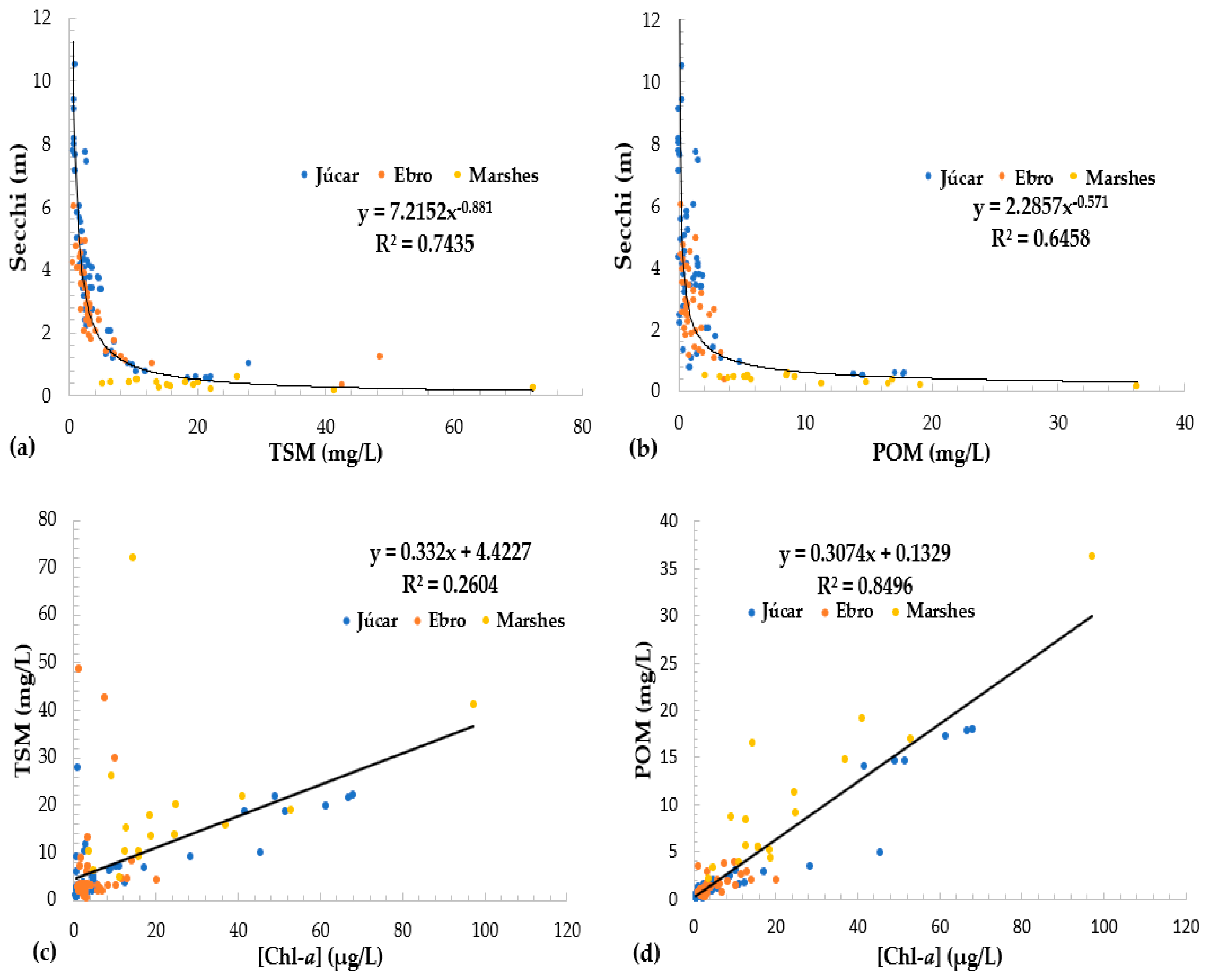
3.1. Field Data Study

To obtain information about the influence of each variable on the transparency of the water, in a first analysis the relationship was studied between Secchi disk depth (SDD) (and [Chl-a]) with organic and total suspended matter (Figure 5) of all in situ measured points. As can be seen, both TSM and POM have a strong inverse correlation with SD (Figure 5a,b). From this, it can be deduced that, in these reservoirs, the transparency of the water is fundamentally influenced by the suspended solids, both mineral and organic.

For the relationship with [Chl-a], POM has higher correlation than TSM (Figure 5c,d). As shown, the POMs that present the highest correlation with chlorophyll are those belonging to the Júcar reservoirs and the Marshes of Albufera, indicating that most of the solids in these areas are phytoplankton and detritus. However, between [Chl-a] and TSM there is lower correlation, especially in those water bodies where [Chl-a] values are low (Ebro reservoirs) (Figure 5c).

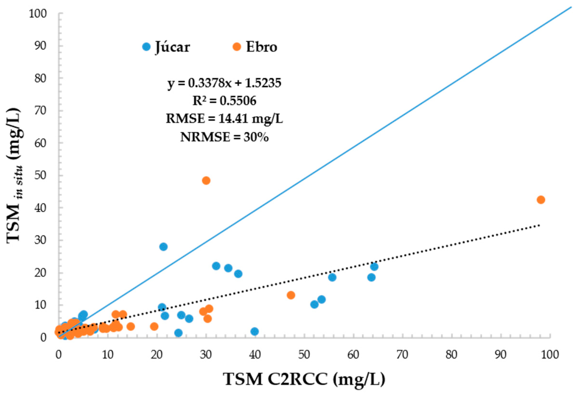
3.2. C2RCC Automatic Processor for Water Quality Products

With the objective of making an independent validation of the automatic product of TSM provided by the atmospheric correction C2RCC in SNAP, Figure 6 shows that the TSM results provided by the processor are positively distributed and show a good correlation with the TSM data measured in the field, presenting an error (RMSE) of 14.4 mg/L. This error can be reduced to 5.3 mg/L using the equation presented in Figure 6. Field data is approximately 1/3 of the data offered by the automatic TSM product.

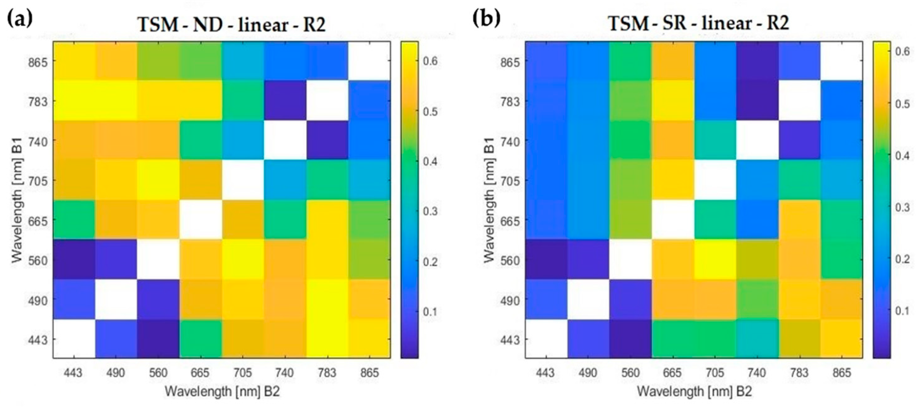
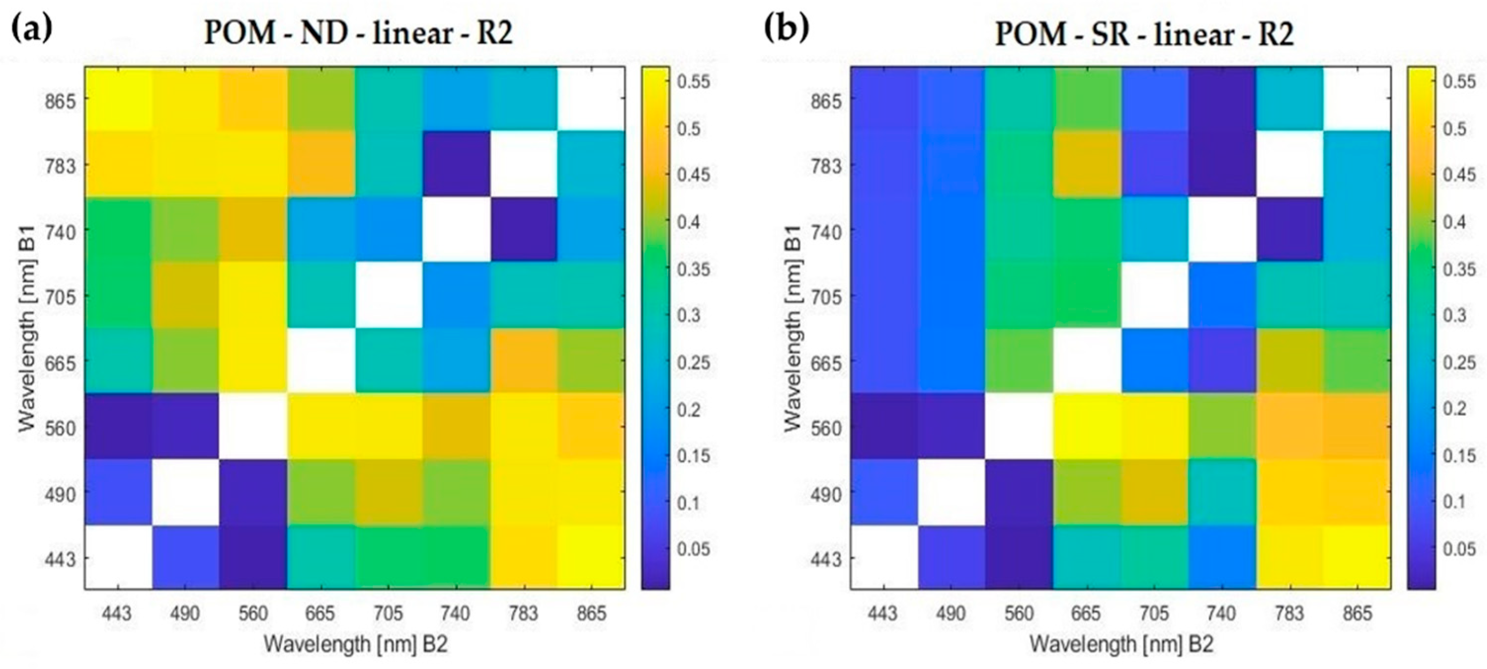
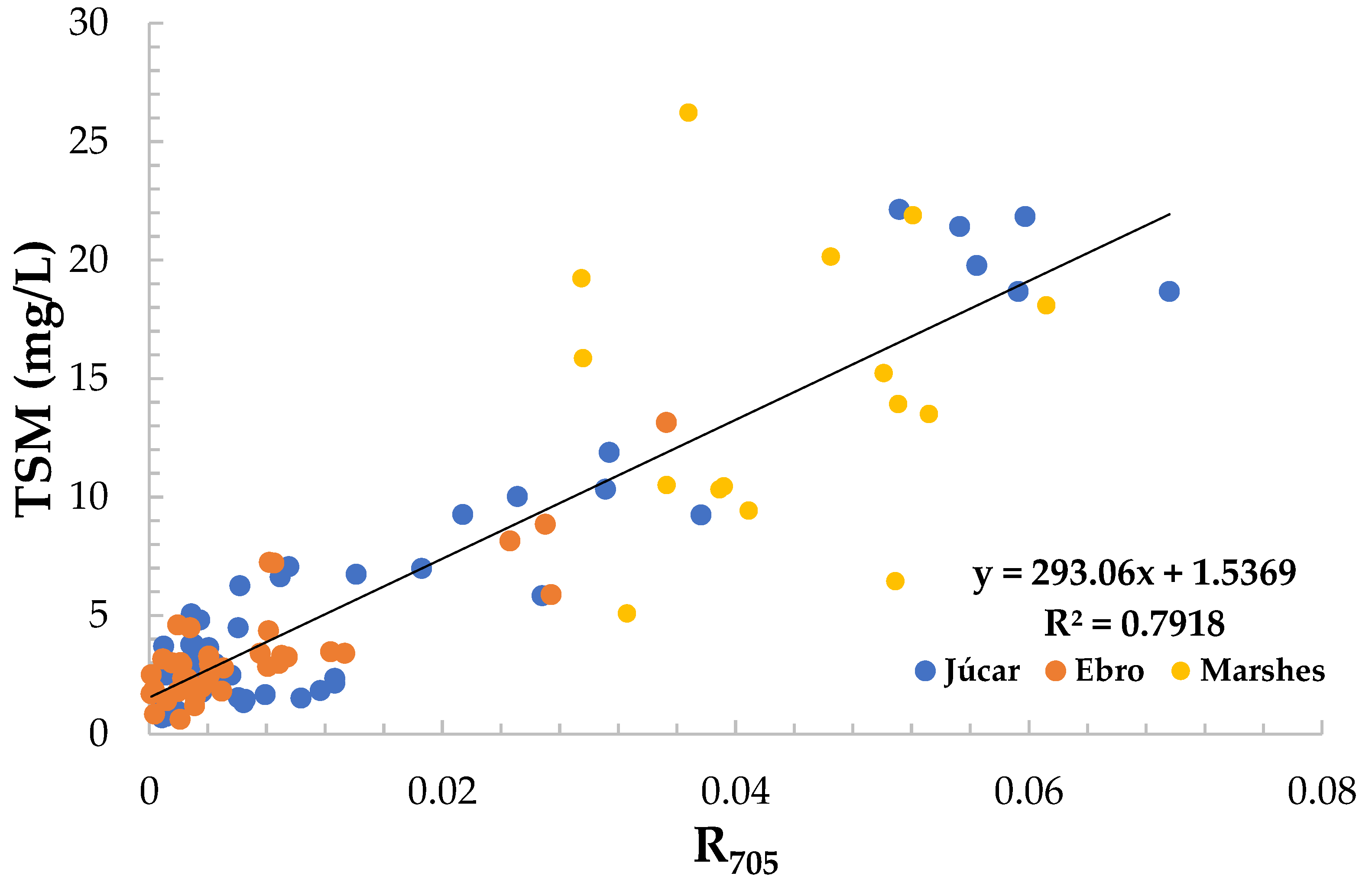
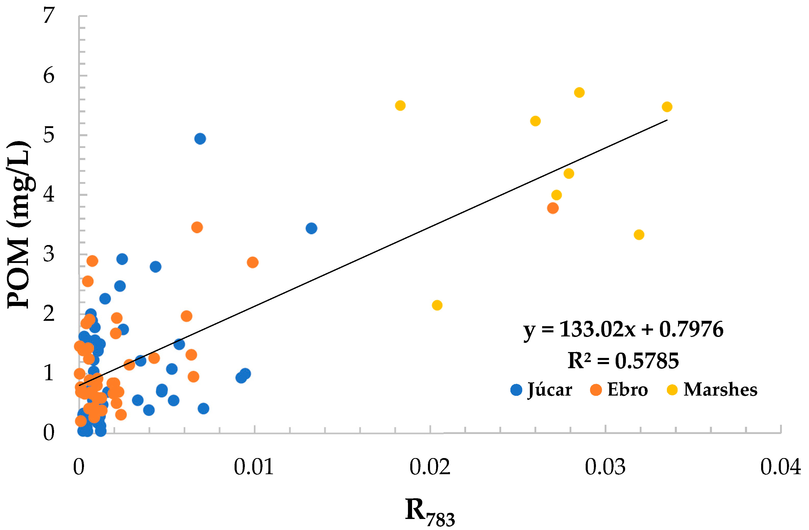
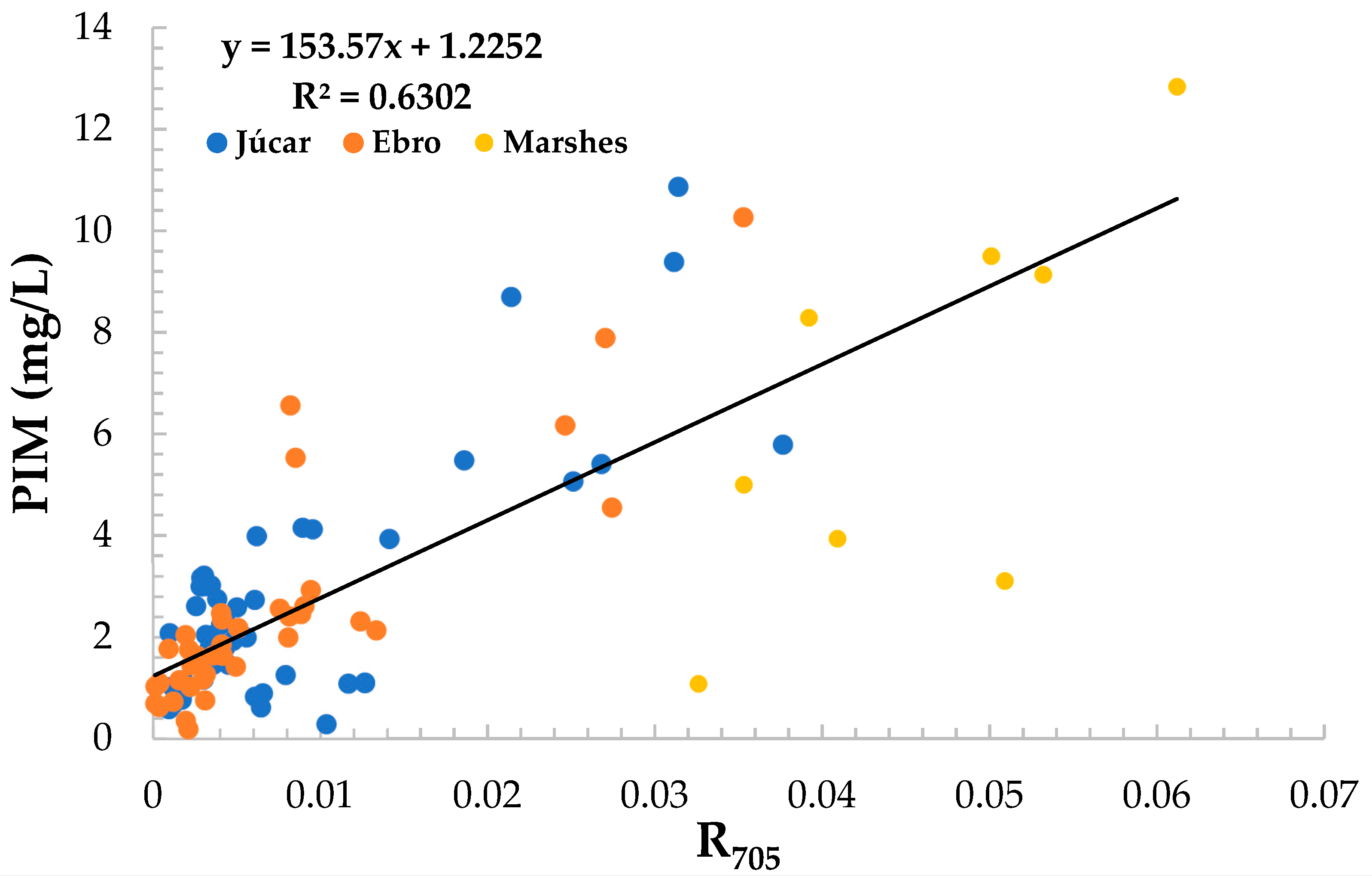
3.3. Algorithms Retrieval

In order to find the best algorithms that can estimate TSM, PIM and POM separately, the correlations between the reflectance obtained from the satellite images and the variables measured have been calculated. First, we decided to test the combinations using all the data of the three variables. The regression between the field data and the estimated results were too low (R² < 0.3), so we decided to reduce the concentration range of used samples. After various adjustments and tests, the best combinations were extracted for TSM with values lower than 30 mg/L, for POM with values lower than 6 mg/L and for PIM with values lower than 13 mg/L. For all the results, the best fitting function turned out to be the linear adjustment.

Once the results are obtained, the ARTMO toolbox provides us their correlation matrices, through a heatmap that indicates the correlation coefficients between the factors in a more visual way, for all possible band combinations. As can be seen in Figure 7 and Figure 8, the correlations presented by the bands, used for developing the different algorithms, positively determine their quality.

Results relating measured values of these three studied variables and different band combinations, and error statistics results relating measured and estimated values are summarized together in

Table 2. Algorithm results for TSM. Only the best 10 results are shown.

Band Comb. (x)	Formula (y = TSM in mg/L)	R2	RMSE (mg/L)	NRMSE (%)
705	y = 293.06x + 1.5369	0.7918	2.7	10.3
783	y = 454.58x + 2.7696	0.6829	3.3	12.7
740	y = 459.41x + 2.6277	0.6682	3.4	13.0
$\frac{443-783}{443+783}$	y = −12.42x + 13.62	0.6377	3.6	13.6
$\frac{490-783}{490+783}$	y = −13.51x + 15.411	0.6353	3.6	13.6
$\frac{560-705}{560+705}$	y = −13.752x + 13.585	0.6275	3.6	13.8
$\frac{705}{560}$	y = 11.407x + 1.6564	0.6169	3.7	13.9
$\frac{443-865}{443+865}$	y = −13.947x + 16.298	0.5930	3.8	14.4
$\frac{560-783}{560+783}$	y = −15.573x + 17.901	0.5891	3.8	14.4
$\frac{865}{443}$	y = −13.299x + 3.1289	0.5522	4.0	15.1

(TSM),

Table 3. Algorithm results for POM. Only the best 10 results are shown.

Band Comb. (x)	Formula y = POM in mg/L	R2	RMSE (mg/L)	NRMSE (%)
783	y = 133.02x + 0.7976	0.5785	0.84	14.75
$\frac{665}{560}$	y = 4.0442x + 0.0715	0.5619	0.86	15.04
$\frac{443-865}{443+865}$	y = −4.0683x + 4.716	0.5611	0.86	15.05
$\frac{865}{443}$	y = −4.5634x + 0.7954	0.5563	0.87	15.13
740	y = −129.97x + 0.7707	0.5543	0.87	15.17
$\frac{705}{560}$	y = 3.1611x + 0.5007	0.5395	0.88	15.42
$\frac{783}{443}$	y = 3.3831x + 0.6307	0.5333	0.89	15.52
$\frac{560-705}{560+705}$	y = −3.4773x + 3.5726	0.5328	0.89	15.53
$\frac{560-783}{560+783}$	y = −4.491x + 5.1542	0.5317	0.89	15.55
$\frac{490-865}{490+865}$	y = 4.3313x + 5.1168	0.5309	0.89	15.56

(POM) and

Table 4. Algorithm results for PIM. Only the best 10 results are shown.

Band Comb. (x)	Formula y = PIM in mg/L	R2	RMSE (mg/L)	NRMSE (%)
705	y = 153.57x + 1.2252	0.6302	1.56	12.17
783	y = 210.75x + 1.9694	0.3472	2.08	16.17
740	y = 208.06x + 1.9144	0.3424	2.08	16.23
$\frac{665}{560}$	y = 5.7616x + 0.9984	0.2918	2.16	16.84
$\frac{560-705}{560+705}$	y = −4.905x + 5.9536	0.2717	2.19	17.08
$\frac{443-865}{443+865}$	y = −5.4007x + 7.2749	0.2561	2.22	17.26
$\frac{490-783}{490+783}$	y = −5.0836x + 6.8363	0.247	2.23	17.36
$\frac{705}{560}$	y = 4.029x + 1.7254	0.2269	2.26	17.59
$\frac{865}{443}$	y = 5.6585x + 0.2233	0.2233	2.26	17.64
$\frac{560-783}{560+783}$	y = −5.1331x + 7.1515	0.18	2.32	18.12

(PIM). The best 10 results are shown for each variable, these being the ones that presented a higher R² and lower RMSE.

Results using only data from 0.6 mg/L to 30 mg/L for TSM, have demonstrated that combining bands located between 443–865 nm the errors obtained between data measured in situ and estimated data are less than 4 mg/L. Even only using the bands located in the red-edge region, this error could be reduced up to 2.7 mg/L. The reflectance in 705 nm (R₇₀₅) is the one that presents the best correlation with the TSM as shown in Figure 9. It is observed that, adjusting by the method of least squares to a linear fitting function, the best adjustment is obtained with the equation:

TSM (mg/L) = 293.06 R₇₀₅ + 1.5369

(3)

Reservoirs located in the Ebro watershed are those with the lowest amounts of suspended solids, while the Albufera marshes have the highest values. Reservoirs located in the Júcar watershed present more varied values.

For the organic fraction (POM) of TSM (Table 3), the best algorithms using only data from 0.0035 mg/L to 6 mg/L were the simple band R₇₈₃ and the R₆₆₅/R₅₆₀ ratio, with errors of 0.84 mg/L and 0.86 mg/L between the measured and estimated data.

Figure 10 shows the correlation between R₇₈₃ and the in situ data. In this case it has been adjusted by the method of least squares to a linear fitting function, to obtain the best adjustment with the following equation:

POM (mg/L) = 133.02 R₇₈₃ + 0.7976

(4)

For PIM, it emerged that R₇₀₅ is the one that presents the best correlation (shown in Figure 11) with an error of 1.56 mg/L between measured and estimated data.

Adjusting by the method of least squares to a linear fitting function, the best adjustments are obtained with the equation:

PIM (mg/L) = 153.57 R₇₀₅ + 1.2252

(5)

From Figure 10 and Figure 11, can be seen that the Ebro and Júcar watershed reservoirs have inorganic sediment predominance, whereas in the marshes the organic component dominates.

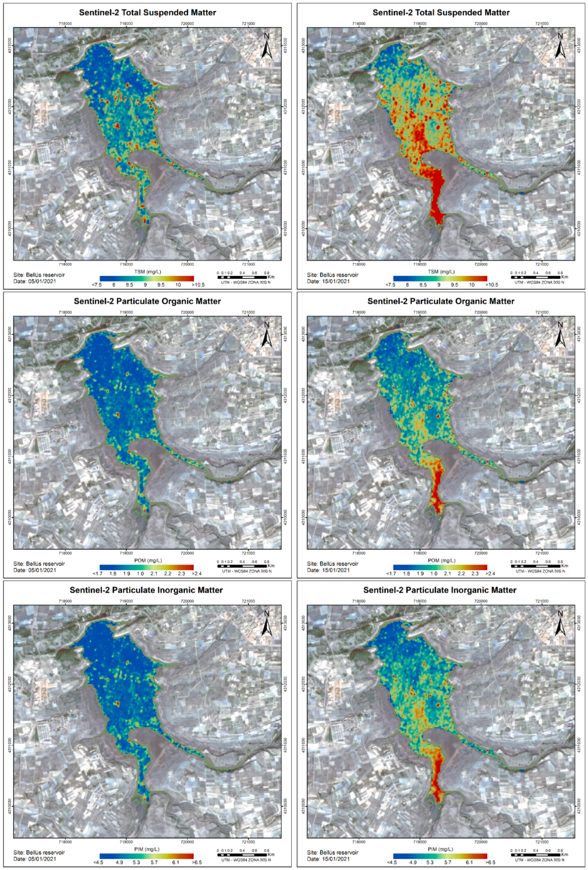
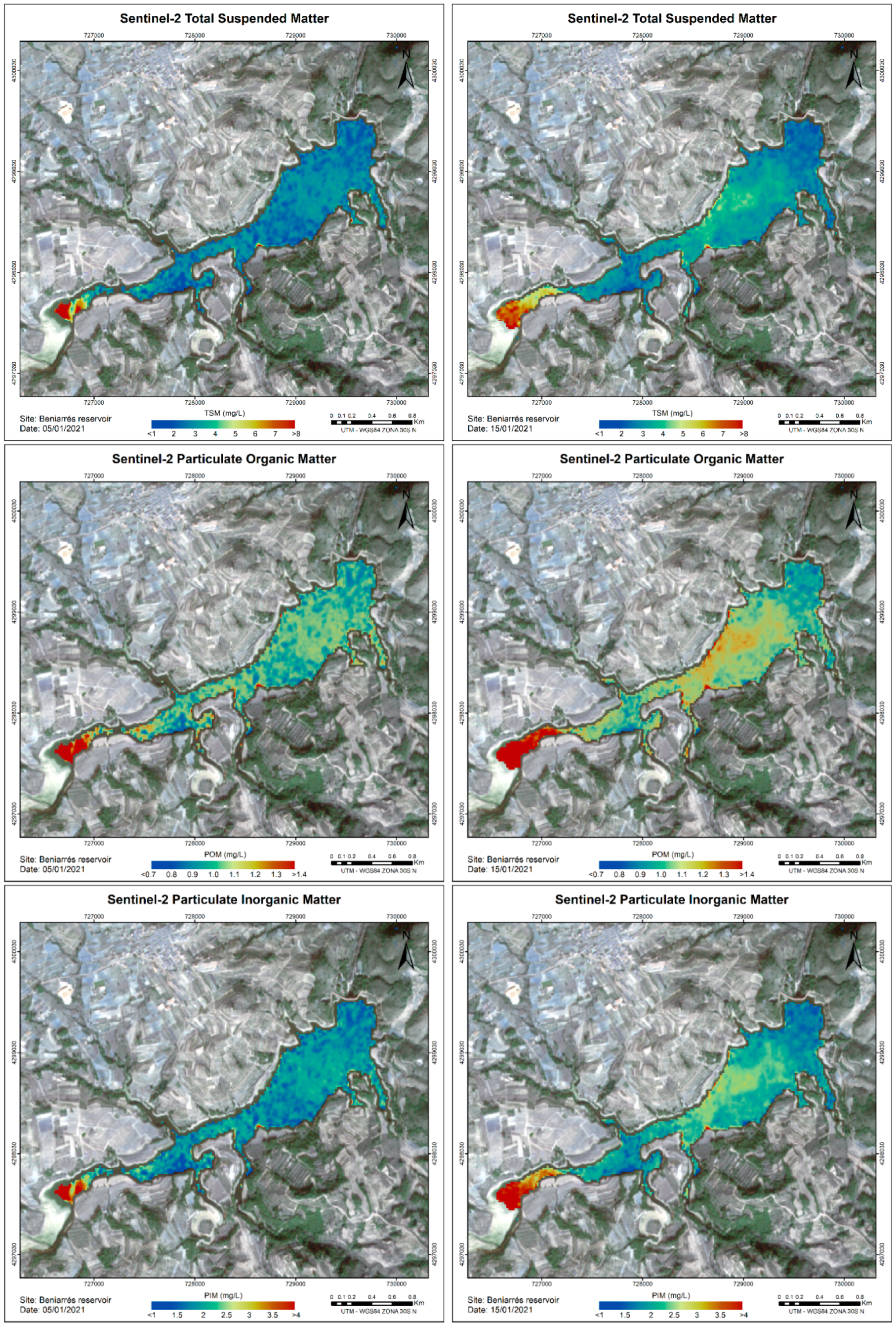
3.4. Mapping TSM, POM and PIM Using New Algorithms for Sentinel-2 Imagery

As an example, Figure 12 and Figure 13 show two reservoirs chosen from the studied sampling points, with different trophic status and from which maps have been obtained for each variable included in this study. For this, from an S2-Level1C image, resampled to 20 m, trimmed and subsequently corrected with C2RCC, Equations (3)–(5) have been applied. A 3 × 3 average filter has also been applied to the obtained maps, to correct the “salt and pepper” effect provided by the atmospheric corrector.

The selected dates correspond to before 5 January 2021 and after 15 January 2021, a heavy rain episode. Thus, it is possible to observe both the contributions that may have been produced in the reservoirs and the distribution patterns. In both reservoirs, the dam is in the most northern part. As can be observed, the three variables follow the same distribution pattern, accumulating the highest values in the inflow area of the reservoir and leaving the area of the dam cleaner. However, one predominates over another depending on the image. Heavy rain episodes increase the quantity of TSM of both reservoirs, but the relationship between the organic and inorganic fractions maintains a similar proportion.

4. Discussion

Turbidity is an optical property of water that partially scatters light. Suspended sediments are responsible for most of said scattering. Ergo, the more suspended particles, the higher the water’s turbidity. The bands more appropriate for TSM estimation, as discussed in Ruddick et al. [55], depend on its concentration, and for high TSM concentrations the best results are obtained with longer wavelengths (700 nm and beyond). Curran et al. [56] and Novo et al. [57] demonstrated that single band algorithms could be accepted where TSM augments with increasing reflectance. Despite that, according to Doxaran et al. [58], composite matter in water changes the reflectance of the water body, implying variation in colors, and thus different spectral bands’ combinations might be used for TSM estimation. Many studies often use a single red band (625–700 nm) for TSM estimation. Even so, it should be noted that the efficiency of these algorithms diminishes in areas with extreme sediment loads where radiometric measurements in the red band no longer correlate with increases in TSM, because a saturation effect can occur according to Luo et al. [59]. Some authors such as Novoa et al. [60] state that, to avoid these limitations, multiband models based on the relationship of bands must be developed and applied.

In our study, the data range for which the TSM estimation algorithms were obtained is 0.6 mg/L to 30 mg/L. Most of the algorithms obtained have been formulated with combinations between bands ranging from 443 to 842 nm; nevertheless, the best result was obtained using only the simple band R₇₀₅. Sòria-Perpinyà et al. [61] use a range of TSM similar to ours, with concentrations under 20 mg/L. Their results, also using MSI-S2 imagery, obtained with a R₇₀₀ band algorithm present a R² 0.85, RMSE 1.55 mg/L and NRMSE 7.8 %. In this same study, an algorithm based on R₇₈₃/R₄₉₂ combination was obtained, but in this case the concentrations were above 20 mg/L. TSM has also been estimated using the reflectance peak near 700 nm, from sensors such as MERIS, in relatively low concentrations <32 g/m³ (R² > 0.81) in the studies of Härma et al. [62], Kallio et al. [63] and Koponen et al. [64]. Doxaran et al. [65], using the ratio 850/550 for highly turbid waters (<985 mg/L), show the high potential of NIR bands for TSM estimation, but exhibiting a strong non-linear correlation. For the MSI-S2, this ratio did not give significant results, which may be due to the fact that the concentrations are much lower.

Several bio-optical algorithms have been created to estimate the Particulate Organic Carbon (POC) concentration in oceanic layers [66,67,68,69,70] and eutrophic lakes [71]. These algorithms were obtained for band ratios corresponding to red-to-blue (R₆₆₅/R₄₉₀), red-to-green (R₆₆₅/R₅₆₀), or blue-to-red (R₄₉₀/R₆₆₅) for ocean studies and for blue-to-green (R₄₄₃/R₅₆₀ and R₄₉₀/R₅₆₀) ratios for lake studies. Besides, systems with an organic prevalence whose spectral signatures stem from algae concentrations sharing the pronounced absorption features and backscatter peaks described for chlorophyll. Gitelson et al. determined in several studies [72,73] that [Chl-a] has a peak near 700 nm and that this reflectance peak was important for measuring chlorophyll concentrations. Dekker et al. [74] mentioned that the scattering and absorption characteristics of [Chl-a] can also be studied when more than one band is used. Even so, with this study it has been deduced that the band that best estimates the organic fraction of TSM is R₇₈₃. The second-best result for estimating POM in our study, is the ratio 665/560 nm. Algorithms using ratios of reflectance in the blue (~400–500 nm) to that in the green or red (~500–700 nm) have been found to be well correlated with [Chl-a] [75]. Ratios used include MERIS bands 665/550 nm [76]. The red band (665 nm) makes use of the [Chl-a] absorption maximum and acts to normalize the effects of [Chl-a] absorption and backscattering by particulate matter [15].

Algorithms for perceived PIM are very similar to those for TSM (especially in sediments with high inorganic rates) and use red and NIR bands [76,77]. The reason is that inorganic particles contribute greatly to scattering in the NIR [78]. Our study has determined that, for a range of 0.188–12.84 mg/L, PIM can be estimated through the use of the R₇₀₅ band algorithm with a high R². There are several publications [76,77,79] showing that the elevated signals in the NIR part of the spectrum are a good predictor of TSM. Water samples used in these studies were very rich in mineral particles (250 mg/L). Therefore, if the water has a high amount of mineral particles, it is attributed to an elevated NIR signal.

Despite the fact that the automatic products offered by the C2RCC processor may present an acceptable correlation (R² = 0.5506) with the data measured in situ and suitable statistics (RMSE = 14.41 mg/L; NRMSE = 30%), these results can be improved by the algorithms proposed in this study, which present both better correlations (R² = 0.7918) and lower error compared to the real data (RMSE = 2.7 mg/L; NRMSE = 10.3%).

The use of remote sensing as a tool for capturing information applied to Limnology and hydrological planning represents a saving in time and costs for water resources’ evaluation and, therefore, for the management, rationalization, optimization and modernization of hydrological planning. The experience acquired from the beginning of remote sensing programs to the present day in the study and monitoring of Spanish water bodies using multispectral images, indicates the need to incorporate data collection in situ, and to adjust specific algorithms in areas as unique as those chosen for this study.

5. Conclusions

Our results have demonstrated the potential of remote sensing techniques to differentiate POM and PIM and thus map out the composition of suspended particles, in order to provide their spatial and temporal variations. It is important to determine the composition of TSM in the study area given that the transparency of the water is fundamentally influenced by the suspended solids, sometimes the mineral fraction rather than the organic one.

In this work, with statistical significance for continental waters, 10 indices are proposed for the estimation of TSM, 10 indices for the estimation of the POM and one index for the estimation of PIM, found from data obtained in very different water bodies. Results show that the use of a single band (R₇₀₅ for TSM and PIM determination and R₇₈₃ for POM determination) can provide a robust and sensitive algorithm for these variables. The correlations presented by the use of the single band algorithms were R² = 0.7918 for TSM algorithm, R² = 0.5785 for POM algorithm and R² = 0.6302 for PIM algorithm. The normalized errors presented by these algorithms were 10.3% for TSM algorithm, 14.8% for POM algorithm and 12.2% for PIM algorithm. The single band selected algorithms have been verified after application in Sentinel-2 images and in water bodies is viable. The C2RCC processor provides acceptable automatic results regarding TSM determination and could be an alternative to using specific algorithms.

Wind speed, rainfall, human activities or soil type can affect TSM, POM and PIM changes. In future studies, a comprehensive analysis of multiple factors surrounding water bodies would be necessary to determine possible trends in variation. In particular, the application of similar sensors or more advanced sensors would assist in constructing consistent and more complete satellite-derived time series data. In order to deepen the range of application of the algorithms developed, it would be convenient to extend the investigation to a larger number of water bodies with different trophic status (lakes, ponds, reservoirs, marshes, etc.).

References

1. Hestir, E.L.; Brando, V.E.; Bresciani, M.; Giardino, C.; Matta, E.; Villa, P.; Dekker, A.G. Measuring freshwater aquatic ecosystems: The need for a hyperspectral global mapping satellite mission. Remote Sens. Environ. 2015, 167, 181–195. [Google Scholar] [CrossRef] [Green Version]
2. Lehner, B.; Döll, P.; Alcamo, J.; Henrichs, T.; Kaspar, F. Estimating the impact of global change on flood and drought risks in Europe: A continental, integrated analysis. Clim. Chang. 2006, 75, 273–299. [Google Scholar] [CrossRef]
3. Roland, F.; Huszar, V.L.M.; Farialla, V.F.; Enrich-Prast, A.; Amado, A.M.; Ometto, J.P.H.B. Climate change in Brazil: Perspective on the biogeochemistry of inland waters. Braz. J. Biol. 2012, 72, 709–722. [Google Scholar] [CrossRef] [Green Version]
4. Schmugge, T.J.; Kustas, W.P.; Ritchie, J.C.; Jackson, T.J.; Rango, A. Remote sensing in hydrology. Adv. Water Resour. 2002, 25, 1367–1385. [Google Scholar] [CrossRef]
5. Pereira-Sandoval, M.; Urrego, P.; Ruíz-Verdú, A.; Tenjo, C.; Delegido, J.; Sòria-Perpinyà, X.; Vicente, E.; Soria, J.; Moreno, J. Calibration and validation of algorithms for the estimation of chlorophyll-a concentrations and Secchi depth in inland waters with Sentinel-2. Limnetica 2019, 38, 471–487. [Google Scholar]
6. Sòria-Perpinyà, X.; Delegido, J.; Urrego, P.; Pereira-Sandoval, M.; Vicente, E.; Rúiz-Verdú, A.; Soria, J.M.; Peña-Martínez, R.; Tenjo, C.; Moreno, J. Validación de algoritmos para la estimación de la clorofila-a con Sentinel-2 en la Albufera de València. In Teledetección, Nuevas Plataformas y Sensores Aplicados a la Gestión del Agua, Agricultura y Medio Ambiente, Proceedings of the XVII Congreso de la Asociación Española de Teledetección, Murcia, Spain, 3–7 October 2017; Ruiz, L.A., Estornell, J., Erena, M., Eds.; Universidad Politécnica de Valencia: Valencia, Spain, 2017; pp. 289–292. [Google Scholar]
7. Giardino, C.; Pepe, M.; Brivio, P.A.; Ghezzi, P.; Zilioli, E. Detecting chlorophyll, Secchi disk Depth and Surface temperature in a sub-alpine lake using Landsat imagery. Sci. Total Environ. 2001, 268, 19–29. [Google Scholar] [CrossRef]
8. Gitelson, A.; Guirlin, D.; Moses, W.J.; Barrow, T. A bio-optical algorithm for the remote estimation of the chlorophyll-a concentration in case 2 waters. Environ. Res. Lett. 2009, 4, 045003. [Google Scholar] [CrossRef]
9. Ruíz-Verdú, A.; Simis, S.G.H.; De Hoyos, C.; Gons, H.J.; Peña-Martínez, R. An evaluation of algorithms for the remote sensing of cyanobacterial biomass. Remote Sens. Environ. 2008, 112, 3996–4008. [Google Scholar] [CrossRef]
10. Doxaran, D.; Froidefond, J.M.; Castaing, P.; Babin, M. Dynamics of the turbidity maximum zone in a macrotidal estuary (the Gironde, France): Observations from field and MODIS satellite data. Estuar. Coast. Shelf Sci. 2009, 81, 321–332. [Google Scholar] [CrossRef]
11. Kutser, T.; Paavel, B.; Metsamaa, L. Mapping colored dissolved organic matter concentration in coastal waters. Int. J. Remote Sens. 2009, 30, 5843–5849. [Google Scholar] [CrossRef]
12. Olmanson, L.G.; Bauer, M.E.; Brezonik, P.L. A 20-year Landsat water clarity census of Minnesota’s 10,000 lakes. Remote Sens. Environ. 2008, 112, 4086–4097. [Google Scholar] [CrossRef]
13. Petus, C.; Chust, G.; Gohin, F.; Doxaran, D.; Froidefond, J.M.; Sagarminaga, Y. Estimating turbidity and total suspended matter in the Adour River plume (South Bay of Biscay) using MODIS 250-m imagery. Cont. Shelf Res. 2010, 30, 379–392. [Google Scholar] [CrossRef] [Green Version]
14. Matthews, M.W. A current review of empirical procedures of remote sensing in inland and near-coastal transitional waters. Int. J. Remote Sens. 2011, 32, 6855–6899. [Google Scholar] [CrossRef]
15. Dekker, A.G.; Vos, R.J.; Peters, S.W.M. Analytical algorithms for lake water TSM estimation for retrospective analyses of TM and SPOT sensor data. Int. J. Remote Sens. 2002, 23, 15–35. [Google Scholar] [CrossRef]
16. Bilotta, G.S.; Brazier, R.E. Understanding the influence of suspended solids on water quality and aquatic biota. Water Res. 2008, 42, 2849–2861. [Google Scholar] [CrossRef] [PubMed]
17. Miller, R.L.; McKee, B.A. Using MODIS Terra 250 m imagery to map concentrations of total suspended matter in coastal waters. Remote Sens. Environ. 2004, 93, 259–266. [Google Scholar] [CrossRef]
18. Balasubramanian, S.V.; Pahlevan, N.; Smith, B.; Binding, C.; Schalles, J.; Loisel, H.; Gurlin, D.; Greb, S.; Alikas, K.; Randla, M.; et al. Robust algorithm for estimating total suspended solids (TSS) in inland and nearshore coastal waters. Remote Sens. Environ. 2020, 246, 111768. [Google Scholar] [CrossRef]
19. Lloyd, D.S.; Koenings, J.P.; LaPerriere, J.D. Effects of turbidity in fresh waters of Alaska. N. Am. J. Fish. Manag. 1987, 7, 18–33. [Google Scholar] [CrossRef]
20. Ryan, P.A. Environmental effects of sediment on New Zealand streams: A review. N. Z. J. Mar. Freshw. Res. 1991, 25, 207–211. [Google Scholar] [CrossRef]
21. Verstraeten, G.; Poesen, J. Estimating trap efficiency of small reservoirs and ponds: Methods and implications for the assessment of sediment yield. Prog. Phys. Geogr. 2000, 24, 219–251. [Google Scholar] [CrossRef]
22. Kulkarni, A. Water Quality Retrieval from Landsat TM Imagery. Complex Adpt. Syst. Model 2011, 6, 475–480. [Google Scholar] [CrossRef] [Green Version]
23. Samboni, N.E.; Carvajal, Y.; Escobar, J. Revisión de parámetros fisicoquímicos como indicadores de calidad y contaminación del agua. Rev. Ing. Investig. 2007, 27, 172–181. [Google Scholar]
24. Kratzer, S.; Kyriliuk, D.; Brockmann, C. Inorganic suspended matter as an indicator of terrestrial influence in Baltic Sea coastal areas—Algorithm development and validation, and ecological relevance. Remote Sens. Environ. 2020, 237, 111609. [Google Scholar] [CrossRef]
25. Schartau, M.; Riethmüller, R.; Flöser, G.; van Beusekom, J.E.E.; Krasemann, H.; Hofmeister, R.; Wirtz, K. On the separation between inorganic and organic fractions of suspended matter in a marine coastal environment. Prog. Oceanogr. 2019, 171, 231–250. [Google Scholar] [CrossRef]
26. Kutser, T.; Paavel, B.; Verpoorter, C.; Ligi, M.; Soomets, T.; Toming, K.; Casal, G. Remote Sensing of Black Lakes and Using 810 nm Reflectance Peak for Retrieving Water Quality Parameters of Optically Complex Waters. Remote Sens. 2016, 8, 497. [Google Scholar] [CrossRef]
27. Ferrer, C. El Sistema hidráulico del Ebro. Hidrología y previsión. In Ríos y Ciudades, Proceedings of the Aportaciones para la Recuperación de los Ríos y Riberas de Zaragoza, Zaragoza, Spain, 2002; de la Cal, P., Pellicer, F., Eds.; Universidad de Zaragoza: Zaragoza, Spain, 2002; pp. 181–198. [Google Scholar]
28. Ibañez, C.; Prat, N.; Canicio, A. Changes in the hydrology and sediment transport produced by large dams on the lower Ebro river and its estuary. Regul. Rivers Res. Manag. 1996, 12, 51–62. [Google Scholar] [CrossRef]
29. Batalla, R.M.; Gómez, C.M.; Kondolf, G.M. Reservoir-induced hydrological changes in the Ebro River basin (NE Spain). J. Hydrol. 2004, 290, 117–136. [Google Scholar] [CrossRef]
30. Losada, J.A.; Ibarra, P.; Echevarría, M.T.; Bermejo, J.L.; Ballarín, D.; Mora, D.; Del Valle, J.; Ollero, A.; Sánchez, M.; Peña, J.L.; et al. Los paisajes de la cuenca del Ebro: Tipologías y análisis paisajístico de sus principales embalses. In Naturaleza Aragonesa: Revista de la Sociedad de Amigos del Museo Paleontológico de la Universidad de Zaragoza; Sociedad de Amigos del Museo Paleontológico de la Universidad de Zaragoza: Zaragoza, Spain, 2013; Volume 30, pp. 52–62. [Google Scholar]
31. SIT Ebro. Available online: http://iber.chebro.es/SitEbro/sitebro.aspx (accessed on 18 February 2021).
32. CHJ. Esquema provisional de temas importantes. Distrito de la Cuenca del río Júcar. In Confederación Hidrográfica del Júcar; Environment Ministry: Valencia, Spain, 2009. [Google Scholar]
33. Martínez, J.F.; Correcher, E.; Piñón, A.; Martínez, M.A.; Pujante, A.M. Estudio del estado ecológico de los ríos de la cuenca hidrográfica del Júcar (España) mediante el índice BMWP. Limnetica 2004, 23, 331–346. [Google Scholar]
34. Paredes-Arquiola, J.; Andreu-Álvarez, J.; Martín-Monerris, M.; Solera, A. Water quantity and quality models applied to the Jucar River Basin, Spain. Water Resour. Manag. 2010, 24, 2759–2779. [Google Scholar] [CrossRef] [Green Version]
35. Andreu, J.; Ferrer-Polo, J.; Pérez, M.A.; Solera, A.; Paredes-Arquiola, J. Drought planning and management in the Júcar River Basin. In Drought in Arid and Semi-Arid Regions; Schwabe, K., Albiac, J., Connor, J., Hassan, R., Meza, L., Eds.; Springer: Dordrecht, The Netherlands, 2013; pp. 237–249. [Google Scholar] [CrossRef]
36. SIA Júcar. Available online: https://aps.chj.es/siajucar/ (accessed on 18 February 2021).
37. Sòria-Perpinyà, X.; Urrego, P.; Pereira-Sandoval, M.; Ruiz-Verdú, A.; Soria, J.M.; Delegido, J.; Vicente, E.; Moreno, J. Monitoring water transparency of a hypertrophic lake (the Albufera of València) using multitemporal Sentinel-2 satellite images. Limnetica 2020, 39, 373–386. [Google Scholar] [CrossRef]
38. Soria, J.; Jover, M.; Domínguez-Gómez, J.A. Influence of Wind on Suspended Matter in the Water of the Albufera of Valencia (Spain). J. Mar. Sci. Eng. 2021, 9, 343. [Google Scholar] [CrossRef]
39. Soria, J.; Vera-Herrera, L.; Calvo, S.; Romo, S.; Vicente, E.; Sahuquillo, M.; Sòria-Perpinyà, X. Residence Time Analysis in the Albufera of Valencia, a Mediterranean Coastal Lagoon, Spain. Hydrology 2021, 8, 37. [Google Scholar] [CrossRef]
40. Caballero, I.; Navarro, G. Análisis multisensor para el estudio de los patrones de turbidez en el estuario del Guadalquivir. Rev. Teledetección 2016, 46, 1–17. [Google Scholar] [CrossRef] [Green Version]
41. Vicente, E.; Hoyos, C.; Sánchez, P.; Cambra, J. Metodología para el establecimiento del estado ecológico según la directiva marco del agua. In Protocolos de Muestreo y Análisis Para Fitoplancton; Confederación Hidrográfica del Ebro, Ministerio de Medio Ambiente: Zaragoza, Spain, 2005. [Google Scholar]
42. Wetzel, R.G.; Likens, G.E. Limnological Analyses, 2nd ed.; Springer: New York, NY, USA, 1991. [Google Scholar]
43. Shoaf, W.T.; Lium, B.W. Improved extraction of chlorophyll a and b from algae using dimethyl sulphoxide. Limnol. Oceanogr. 1976, 21, 926–928. [Google Scholar] [CrossRef]
44. Jeffrey, S.T.; Humphrey, G.F. New spectrophotometric equations for determining chlorophylls a, b, c1 and c2 in higher plants, algae and natural phytoplankton. Biochem. Physiol. Pflanz. 1975, 167, 191–194. [Google Scholar] [CrossRef]
45. APHA. Standard Methods for the Examination of Water and Wastewater, 20th ed.; American Public Health Association: Washington, DC, USA, 1998. [Google Scholar]
46. Drusch, M.; Del Bello, U.; Carlier, S.; Colin, O.; Fernandez, V.; Gascon, F.; Hoersch, B.; Isola, C.; Laberinti, P.; Martimort, P.; et al. Sentinel-2: ESA’s Optical High-Resolution Mission for GMES Operational Services. Remote Sens. Eviron. 2012, 120, 25–36. [Google Scholar] [CrossRef]
47. Pereira-Sandoval, M.; Ruescas, A.; Urrego, P.; Rúiz-Verdú, A.; Delegido, J.; Tenjo, C.; Sòria-Perpinyà, X.; Vicente, E.; Soria, J.M.; Moreno, J. Evaluation of Atmospheric Correction Algorithms over Spanish Inland Waters for Sentinel-2 Multi Spectral Imagery Data. Remote Sens. 2019, 11, 1469. [Google Scholar] [CrossRef] [Green Version]
48. Kutser, T. The possibility of using the Landsat image archive for monitoring long time trends in coloured dissolved organic matter concentration in lake waters. Remote Sens. Environ. 2012, 123, 334–338. [Google Scholar] [CrossRef]
49. Brockmann, C.; Roland, D.; Marco, P.; Kerstin, S.; Sabine, E.; Ruescas, A. Evolution of the C2RCC neural network for Sentinel 2 and 3 for the retrieval of ocean colour products in normal and extreme optically complex waters. In Proceedings of the Living Planet Symposium, Prague, Czech Republic, 9–13 May 2016; Ouwehand, L., Ed.; ESA: São Paulo, Brazil, 2016. [Google Scholar]
50. Louis, J.; Debaecker, V.; Pflug, B.; Main-Knorn, M.; Bieniarz, J.; Mueller-Wilm, U.; Cadau, E.; Gascon, F. Sentinel-2 Sen2Cor: L2A processor for users. In Proceedings of the Living Planet Symposium, Prague, Czech Republic, 9–13 May 2016; ESA: São Paulo, Brazil, 2016. [Google Scholar]
51. Ruescas, A.B.; Pereira-Sandoval, M.; Tenjo, C.; Rúiz-Verdú, A.; Steinmetz, F.; De Keukelaere, L. Sentinel-2 Atmospheric Correction Inter-comparison over two lakes in Spain and Peru-Bolivia. In Proceedings of the Colour and Light in the Ocean from Earth Observation (CLEO) Workshop, Frascati, Italy, 6–8 September 2016. [Google Scholar]
52. Chuvieco, E. Fundamentos de Teledetección Espacial; Ediciones Rialp, S.A.: Madrid, Spain, 1996. [Google Scholar]
53. Delegido, J.; Urrego, P.; Vicente, E.; Sòria-Perpinyà, X.; Soria, J.M.; Pereira-Sandoval, M.; Rúiz-Verdú, A.; Peña-Martínez, R.; Moreno, J. Turbidity and Secchi disc Depth with Sentinel-2 in different trophic status reservoirs at the Comunidad Valenciana. Rev. Teledetección 2019, 54, 14–24. [Google Scholar] [CrossRef] [Green Version]
54. Rivera, J.P.; Verrelst, J.; Delegido, J.; Veroustraete, F.; Moreno, J. On the Semi-Automatic Retrieval of Biophysical Parameters Based on Spectral Index Optimization. Remote Sens. 2014, 6, 4927–4951. [Google Scholar] [CrossRef] [Green Version]
55. Ruddick, K.G.; De Cauwer, V.; Park, Y.J.; Moore, G. Seaborne measurements of near infrared water-leaving reflectance. The similarity spectrum for turbid waters. Limnol. Oceanogr. 2006, 51, 1167–1179. [Google Scholar] [CrossRef] [Green Version]
56. Curran, P.; Hansom, J.; Plummer, S.; Pedley, M. Multispectral remote sensing of nearshore suspended sediments: A pilot study. Int. J. Remote Sens. 1987, 8, 103–112. [Google Scholar] [CrossRef]
57. Novo, E.; Hansom, J.; Curran, P. The effect of viewing geometry and wavelength on the relationship between reflectance and suspended sediment concentration. Int. J. Remote Sens. 1989, 10, 1357–1372. [Google Scholar] [CrossRef]
58. Doxaran, D.; Froidefond, J.M.; Lavender, S.; Castaing, P. Spectral signature of highly turbid waters: Application with SPOT data to quantify suspended particulate matter concentrations. Remote Sens. Environ. 2002, 81, 149–161. [Google Scholar] [CrossRef]
59. Luo, Y.; Doxaran, D.; Ruddick, K.; Shen, F.; Gentili, B.; Yan, L.; Huang, H. Saturation of water reflectance in extremely turbid media based on field measurements, satellite data and bio-optical modelling. Opt. Express 2018, 26, 10435–10451. [Google Scholar] [CrossRef] [PubMed] [Green Version]
60. Novoa, S.; Doxaran, D.; Ody, A.; Vanhellemont, Q.; Lafon, V.; Lubac, B.; Gernez, P. Atmospheric corrections and multi-conditional algorithm for multi-sensor remote sensing of suspended particulate matter in low-to-high turbidity levels coastal waters. Remote Sens. 2017, 9, 61. [Google Scholar] [CrossRef] [Green Version]
61. Sòria-Perpinyà, X.; Vicente, E.; Urrego, P.; Pereira-Sandoval, M.; Tenjo, C.; Ruíz-Verdú, A.; Delegido, J.; Soria, J.M.; Peña-Martínez, R.; Moreno, J. Validation of Water Quality Monitoring Algorithms for Sentinel-2 and Sentinel-3 in Mediterranean Inland Waters with In Situ Reflectance Data. Water 2021, 13, 686. [Google Scholar] [CrossRef]
62. Härma, P.; Vepsalainen, J.; Hannonen, T.; Pyhalahti, T.; Kamari, J.; Kallio, K.; Eloheimo, K.; Koponen, S. Detection of water quality using simulated satellite data and semi-empirical algorithms in Finland. Sci. Total Environ. 2001, 268, 107–121. [Google Scholar] [CrossRef]
63. Kallio, K.; Kutser, T.; Hannonen, T.; Koponen, S.; Pulliainen, J.; Vepsalainen, J.; Pyhalahti, T. Retrieval of water quality from airbone imaging spectrometry of various lake types in different seasons. Sci. Total Environ. 2001, 268, 59–77. [Google Scholar] [CrossRef]
64. Koponen, S.; Attila, J.; Pulliainen, J.; Kallio, K.; Pyhalahti, T.; Lindfors, A.; Rasmus, K.; Hallikainen, M. A case study of airborne and satellite remote sensing of a spring bloom event in the Gulf of Finland. Cont. Shelf Res. 2007, 27, 228–244. [Google Scholar] [CrossRef]
65. Doxaran, D.; Froidefond, J.M.; Castaing, P. A reflectance band ratio used to estimate suspended matter concentrations in sediment-dominated coastal waters. Int. J. Remote Sens. 2002, 23, 5079–5085. [Google Scholar] [CrossRef]
66. Stramski, D.; Reynolds, R.A.; Kahru, M.; Mitchell, B.G. Estimation of particulate organic carbon in the ocean from satellite remote sensing. Science 1999, 285, 239–242. [Google Scholar] [CrossRef] [PubMed]
67. Mishonov, A.V.; Gardner, W.D.; Jo Richardson, M. Remote sensing and surface POC concentration in the south atlantic. Deep Sea Res. Part II Top. Stud. Oceanogr. 2003, 50, 2997–3015. [Google Scholar] [CrossRef]
68. Gardner, W.D.; Mishonov, A.V.; Richardson, M.J. Global poc concentrations from in-situ and satellite data. Deep Sea Res. Part II Top. Stud. Oceanogr. 2006, 53, 718–740. [Google Scholar] [CrossRef]
69. Son, Y.B.; Gardner, W.D.; Mishonov, A.V.; Richardson, M.J. Multispectral remote-sensing algorithms for particulate organic carbon (poc): The gulf of Mexico. Remote Sens. Environ. 2009, 113, 50–61. [Google Scholar] [CrossRef] [Green Version]
70. Kien, T.; Duforêt-Gaurier, L.; Vantrepotte, V.; Schaffer, D.; Mériaux, X.; Cauvin, A.; Fanton, O.; Loisel, H. Deriving particulate organic carbon in coastal waters from remote sensing: Inter-comparison exercise and development of a maximum band-ratio approach. Remote Sens. 2019, 11, 2849. [Google Scholar] [CrossRef] [Green Version]
71. Jiang, G.; Ma, R.; Loiselle, S.; Duan, H.; Su, W.; Cai, W.; Huang, C.; Yang, J.; Yu, W. Remote sensing of particulate organic carbon dynamics in a eutrophic lake (Taihu Lake, China). Sci. Total Environ. 2015, 532, 245–254. [Google Scholar] [CrossRef]
72. Gitelson, A. The peak near 700 nm on radiance spectra of algae and water. Relationships of its magnitude and position with chlorophyll concentration. Int. J. Remote Sens. 1992, 13, 3367–3373. [Google Scholar] [CrossRef]
73. Gitelson, A.; Dall’Olmo, G.; Moses, W.; Rundquist, D.C.; Barrow, T.; Fisher, T.R.; Gurlin, D.; Holz, J. A simple semi-analytical model for remote estimation of chlorophyll-a in turbid waters: Validation. Remote Sens. Environ. 2008, 112, 3582–3593. [Google Scholar] [CrossRef]
74. Dekker, A.G.; Malthus, T.J.; Seyhan, E. Quantitative modelling of inland water quality for high-resolution MSS systems. IEEE Trans. Geosci. Remote Sens. 1991, 29, 89–95. [Google Scholar] [CrossRef]
75. Kutser, T.; Arst, H.; Mäekivi, S.; Kallaste, K. Estimation of the water quality of the Baltic Sea and lakes in Estonia and Finland by passive optical remote sensing measurements on board vessel. Lake Reserv. Manag. 1998, 3, 53–66. [Google Scholar] [CrossRef]
76. Ammenberg, P.; Flink, P.; Lindell, T.; Pierson, D.; Strombeck, N. Bio-optical modelling combined with remote sensing to asses water quality. Int. J. Remote Sens. 2002, 23, 1621–1638. [Google Scholar] [CrossRef]
77. Doxaran, D.; Cherukuru, R.; Lavender, S. Use of reflectance band ratios to estimate suspended and dissolved matter concentrations in estuarine waters. Int. J. Remote Sens. 2005, 26, 1763–1770. [Google Scholar] [CrossRef]
78. Doxaran, D.; Babin, M.; Leymarie, E. Near-infrared light scattering by particles in coastal waters. Opt. Express 2007, 15, 12834–12849. [Google Scholar] [CrossRef] [PubMed]
79. Doxaran, D.; Froidefond, J.M.; Castaing, P. Remote sensing reflectance of turbid sediment-dominate waters. Reduction of sediment type variations and changing illumination conditions effects by use of reflectance ratios. Appl. Opt. 2003, 42, 2623–2634. [Google Scholar] [CrossRef]
Figure 1. Location of selected reservoirs in the Ebro hydrographic watershed. Modified from [31].
Water 13 02453 g001
Figure 2. Location of selected reservoirs in the Júcar hydrographic watershed. Modified from [36].
Water 13 02453 g002
Figure 3. Marshes site sampling location in Albufera of Valencia Natural Park from an RGB composition of the S2 image dated 5 January 2021.
Water 13 02453 g003
Figure 4. Algorithms developing flowchart.
Water 13 02453 g004
Figure 5. SDD as a function (a) Concentration of TSM and (b) Concentration of POM for the different in situ values. (c) Concentration of TSM and (d) Concentration of POM as a function of [Chl-a] for the in situ values.
Water 13 02453 g005
Figure 6. Correlation between TSM measured in the Júcar and Ebro reservoirs and TSM given by the C2RCC processor. In blue, line 1:1 is shown.
Water 13 02453 g006
Figure 7. Correlation matrix (measured vs. estimated) for TSM using ND (a) and SR (b) formulations. Yellow combinations are better correlated.
Water 13 02453 g007
Figure 8. Correlation matrix (measured vs. estimated) for POM using ND (a) and SR (b) formulations. Yellow combinations are better correlated.
Water 13 02453 g008
Figure 9. TSM in situ data in function of R705 using all data under 30 mg/L.
Water 13 02453 g009
Figure 10. POM in situ data in function of R783 using all data under 6 mg/L.
Water 13 02453 g010
Figure 11. In situ PIM in function of R705 using all data under 13 mg/L.
Water 13 02453 g011
Figure 12. Bellús reservoir thematic maps for the three studied variables. Note different scales for POM and PIM.
Water 13 02453 g012
Figure 13. Beniarrés reservoir thematic maps for the three variables studied. Note different scales for POM and PIM.
Water 13 02453 g013