
Stratification in a Reservoir Mixed by Bubble Plumes under Future Climate Scenarios
by
 ,
,
David Birt
1,*, 
Danielle Wain
2,3,*,
Emily Slavin
4,
Jun Zang
1,
Robert Luckwell
5 and
Lee D. Bryant
1 1
Department of Architecture & Civil Engineering, University of Bath, Claverton Down, Bath BA2 7AY, UK
2
7 Lakes Alliance, 137 Main Street, Belgrade Lakes, ME 04918, USA
3
Colby College, University of Maine, Mayflower Hill Drive, Waterville, ME 04901, USA
4
Drinking Water Inspectorate, Area 1A, Nobel House, 17 Smith Square, London SW1P 3JR, UK
5
Bristol Water, Bridgwater Road, Bristol BS13 7AT, UK
*
Authors to whom correspondence should be addressed.
Water 2021, 13(18), 2467; https://doi.org/10.3390/w13182467
Submission received: 15 July 2021
/
Revised: 18 August 2021
/
Accepted: 25 August 2021
/
Published: 8 September 2021
(This article belongs to the Special Issue Physical Processes in Lakes)
Abstract
:During summer, reservoir stratification can negatively impact source water quality. Mixing via bubble plumes (i.e., destratification) aims to minimise this. Within Blagdon Lake, a UK drinking water reservoir, a bubble plume system was found to be insufficient for maintaining homogeneity during a 2017 heatwave based on two in situ temperature chains. Air temperature will increase under future climate change which will affect stratification; this raises questions over the future applicability of these plumes. To evaluate bubble-plume performance now and in the future, AEM3D was used to simulate reservoir mixing. Calibration and validation were done on in situ measurements. The model performed well with a root mean squared error of 0.53 °C. Twelve future meteorological scenarios from the UK Climate Projection 2018 were taken and down-scaled to sub-daily values to simulate lake response to future summer periods. The down-scaling methods, based on diurnal patterns, showed mixed results. Future model runs covered five-year intervals from 2030 to 2080. Mixing events, mean water temperatures, and Schmidt stability were evaluated. Eight scenarios showed a significant increase in water temperature, with two of these scenarios showing significant decrease in mixing events. None showed a significant increase in energy requirements. Results suggest that future climate scenarios may not alter the stratification regime; however, the warmer water may favour growth conditions for certain species of cyanobacteria and accelerate sedimentary oxygen consumption. There is some evidence of the lake changing from polymictic to a more monomictic nature. The results demonstrate bubble plumes are unlikely to maintain water column homogeneity under future climates. Modelling artificial mixing systems under future climates is a powerful tool to inform system design and reservoir management including requirements to prevent future source water quality degradation.
1. Introduction
During the summer months, increased atmospheric heating leads to many reservoirs stratifying as increased surface heating creates temperature differences in the water column [1,2]. Reservoir stratification is defined as when there is a temperature gradient within the water column [3]. Thermally stratified water bodies are stable and mixing is suppressed [4]; these physical effects can have considerable influence on the biological, chemical, and general ecosystem processes of the water body [5]. Correspondingly, summer stratification directly affects the water quality within reservoirs [6] via processes including benthic sediment oxygen demand and decomposition of organic matter which consume oxygen from the hypolimnion. When stratification persists for long enough, the inhibition of oxygen supply to the hypolimnion results in oxygen depletion and may result in hypoxic conditions (i.e., the near absence of oxygen at <2 mgL dissolved oxygen). Whether a water body is hypoxic or not drives many critical biogeochemical processes including trace metal transport, phytoplankton dynamics, and the carbon cycle [3,7,8,9].
Artificial destratification (i.e., mixing) is often used in lakes and reservoirs to overcome negative effects of summer stratification [10]. A popular method used is bubble plumes [11]. The reported success of bubble plumes in reservoir management has been varied, suggesting that there is a lack of guidance regarding best operational practice [12]. Bubble plumes are usually installed at the deepest point of the water column and force compressed air into the bottom water, which rises and forms a plume [13]. Bubble plumes work to destratify the water column as the rising bubbles entrain the surrounding denser hypolimnion water. The denser water is then raised into the lighter epilimnion, promoting mixing [14]. This allows aeration via both atmospheric gas exchange and directly from the produced bubbles [15]. Many water utilities use bubble plume destratification systems to ultimately improve source water quality prior to draw-off [16]. A minimum airflow of 9.2 m3 min km has been given as a threshold to ensure total destratification of a reservoir via these plumes [17,18]. The aim of destratification systems such as bubble plumes is to reduce cyanobacteria biomass and minimise concentrations of trace metals, such as soluble manganese, entering the water treatment works to improve the sustainability of treatment and reduce costs to the consumers [16,18]. Oxygenation of the hypolimnion has been shown to decrease concentrations of soluble reduced forms [19] of iron and manganese [20] which are released from sediments under low-oxygen conditions [21]. Additional mixing can affect phytoplankton by increasing the mixed depth to below the photic zone, thereby reducing irradiance which has been shown to reduce cyanobacteria blooms [22].
Currently, increased greenhouse gases (GHG), such as methane (CH4) and carbon dioxide (CO2) [23], are leading to a rapid rise in global temperatures. It has been shown that inland waters (e.g., reservoirs) may account for ∼18% of CH4 emissions globally [24,25]. With existing trends, future GHG release will further contribute to global temperature rise and its consequences. Climate change influences inland water bodies via alterations to air temperature and precipitation [26]. This introduces new elements that threaten to exacerbate water-quality issues related to reservoir stratification [27]. For many reservoirs, there will be alterations to the timing of stratification, potentially forming earlier and destratifying later, leading to enhanced periods of hypolimnetic anoxia and subsequent release of deleterious chemical species from the sediment [27,28,29]. This directly affects carbon fluxes and long-term dissolved organic matter trends by extending anoxic periods in the hypolimnion [27]. Rising global temperatures and increased anthropogenic eutrophication of freshwater systems are likely to promote favourable growth conditions for cyanobacteria. Increased water column stability can favour bloom-forming or positively buoyant species of cyanobacteria, some of which may produce taste and odour compounds or cyanotoxins and result in a deterioration in source water quality [30].
Prolonged stratification seasons predicted with climate change will require destratification systems to be efficient in both current and future climates. In addition, more stable water columns (i.e., stronger stratification) will be increasingly likely, which will require greater energy input from destratification systems to successfully mix lakes and reservoirs [28]. However, the relationship between increased temperature and stratification stability is not a linear effect and stratification can be strongly influenced by water-body morphometry and volume [5]. To date, research has largely focused on the effects of artificial mixing on source water quality in current climates. In this novel study, modelled future climate scenarios were used to estimate how effective current destratification systems are likely to be in the future.
During June 2017, much of western Europe was struck by a heatwave. Record-breaking temperatures were recorded across many countries, including the UK. On 21 June, temperatures in the UK reached 34.5 °C; at the time, this was the hottest June since 1976 [31]. Such heatwaves have been shown to cause strong stratification events in shallow polymictic lakes; several of which are similar in depth to the study site, Blagdon Lake, located in the southwestern UK [32].
This study presents in situ observations of temperature in the shallow, aerated Blagdon Lake during the 2017 heatwave. These observations are used as the basis for the development of a 3D hydrodynamic model, via the widely used AEM3D [33,34,35,36,37] which is available publicly with a yearly licence, to capture effects of extreme events on stratification such as the 2017 summer heatwave. With this calibrated model and down-scaled hourly future forcing data, this study examines how effective bubble plumes will be under future climate scenarios. Results show that existing issues with reservoir mixing interventions will likely continue into the future and managers will need to consider future proofing options.
2. Materials and Methods
2.1. Study Site
Blagdon Lake is a shallow drinking water reservoir, located in Somerset, England, and operated by Bristol Water Plc. The reservoir has a surface area of 1.78 km2 with a mean depth of 4.75 m and a maximum depth of approximately 12 m (Figure 1). The lake was created when the River Yeo was dammed in 1905. Several small streams feed into Blagdon and these inflows have a combined catchment area of 21.8 km2.
Artificial destratification was first implemented in Blagdon in the 1970s and since 2007 there have been seven bubble plumes installed (Figure 1). The bubble plumes are typically operated from April to September each year with the aim of destratifying the reservoir during the summer. Specifically, the bubble plumes were installed at Blagdon to address problems with soluble manganese concentrations and phytoplankton cell counts at the draw-off. Initially, five of the bubble plumes were positioned at 200 m, 250 m, 400 m, 600 m, and 850 m away from the draw-off tower at the dam. An additional two bubble plumes were placed nearer the draw-off tower to reduce soluble manganese concentrations entering the treatment plant. The bubble plumes contain no moving parts and have a 2-meter pipe containing a helical structure where compressed air bubbles can mix with the bottom water and generate a vertical plume that rises to the surface. These bubble plumes have a reported airflow of 0.011 m3s (Bristol Water pers. Comms).
Per data collected by Bristol Water, the bubble plumes appear to have reduced concentrations of soluble manganese at the Blagdon draw-off tower, with a 91.6% reduction from 2007 to 2008 of maximum observed soluble manganese. However, the effects of bubble plumes on phytoplankton cell counts at Blagdon, in particular cyanobacteria, appear less successful. Bloom-forming cyanobacteria are positively buoyant and have specific adaptations, such as gas vacuoles, that provide a competitive advantage under stratified conditions. Generally, the frequency of high counts of bloom-forming cyanobacteria at the Blagdon draw-off have increased since 2006. In 2014, for example, cyanobacteria cell counts at the draw-off exceeded 20,000 cells mL on twelve occasions and peaked at 125,038 cells mL, which related to a Microcystis bloom. On 26 June 2017, counts of Microcystis were elevated at the Blagdon draw-off, following the heatwave. Data provided by Bristol Water indicate that bubble plumes are not fully effective at reducing the buoyancy advantage of bloom-forming cyanobacteria during warm periods [38].
2.2. Observation Methodology
From 20th May to 5th October 2017, two temperature chains were deployed in Blagdon Lake to better understand the thermal regime in the reservoir over this time period. Each of the two chains were set at one-metre resolution and recorded data every ten minutes. One chain was placed in the deeper part of the reservoir (at depth of approximately 9 m), located within the zone immediately influenced by the bubble plumes located at latitude 51.33858 and longitude −2.70858; this chain is hereby referred to as temperature chain 1 (TC1). Per instructions from the water utility, this chain was placed as close as allowed to this intake zone. In order to evaluate the spatial extent of bubble plume mixing, the other temperature chain was placed further away in the shallower (at depth of approximately 5 m), non-aerated section of the reservoir located at latitude 51.33116 and at longitude −2.688. This shallower chain is referred to as temperature chain 2 (TC2). Over the 2017 observation period, a series of Secchi depths were also taken within Blagdon Lake at various points along the bubble plume transect; see Figure 1.
2.3. Data
2.3.1. Boundary Condition Data
To cover the forcing requirements of AEM3D, eight meteorological inputs were used. These include solar radiation (Wm), cloud cover (decimal), air temperature (°C), atmospheric pressure (Pascals), precipitation (mday), wind speed (ms), wind direction (°) and relative humidity (decimal). Information about wind, air temperature, cloud cover and atmospheric pressure was taken from the weather station at Bristol Airport, which is proximal (around 5 km) to Blagdon Lake. Precipitation, solar radiation and relative humidity were sourced from the Filton weather station; this station is further from the lake (20 km) but offers a more comprehensive suite of measured variables than available for Bristol Airport. Weather station positions relative to Blagdon Lake are shown in Figure 2. The Met Office MIDAS Open UK Land Surface Stations Data was used to gather relative humidity, solar radiation and precipitation [39]. Remaining weather variables were sourced from the sub-daily Met Office Hadley Centre’s Integrated Surface Database [40,41,42,43]. Whilst the most proximal sources were considered, the lack of direct meteorological data is a limitation that was taken into account in the evaluation of results but not considered a critical detriment. Mass balance information for the calibration and validation periods were sourced from outflow and reservoir capacity provided by Bristol Water. This calculated inflow was then separated between the six stream inflows into the lake, namely the Yeo, Butcombe, Rickford, Ubley, Copse and Holt Farm; the weighting applied to each inflow was based on the percentage of the lake’s catchment each tributary contributed. Forcing data related to the seven bubble plumes installed in the reservoir was based on their 0.011 m3s flow rate. Modelling was focused on characterising the summer season to cover time periods when stratification was most likely to occur; as such, the bubble plumes were assumed to be on throughout the simulations.
2.3.2. Future Meteorological Data
Future forcing data were sourced from the UK Climate Projection 2018 (UKCP18) project which was designed to help inform adaptions as a result of climactic change [44]. The UKCP18 made use of models from the Coupled Model Intercomparison Project Phase 5 (CMIP5). These data sets were taken from regional climate model projections for the future climate of the UK extending from a 100-year period from 1981 to 2080 [45]. The climate projections were considered for the highest GHG emission scenario used by the IPCC, the representative pathway 8.5 (RCP 8.5). This representative pathway, named for the projected radiative forcing of 8.5 Wm by 2100, predicts a future where high energy demand and high GHG emissions occur with little to no climate change policies to counteract this, thereby worsening climate change; due to this RCP 8.5 is considered the “worst case” scenario [46,47]. These projections were done using the UK Met Office’s Hadley Centre Global Environmental model (HadGEM3), a coupled atmosphere-ocean climate model [48].
Twelve UKCP18 climate scenarios were down-scaled from twelve different HadGEM3-GC3.05 simulations from a grid size of 60 km to a higher resolution of 12 km via the HadREM3-GA705 model covering much of the British Isles on the Ordnance Survey’s British National Grid [45]. The dataset has several separate projections of future climates that were used to force the future model runs; the scenarios used were 1, 4–13 and 15 since these had the required variables. These twelve scenarios offer distinct projections of climate variability due to climate change over the British Isles until 2080. From these projections, the following data were sourced at daily values with the following units: downwards shortwave radiation (Wm), northerly wind speed (ms), easterly wind speed (ms), relative humidity (%), cloud cover (%), atmospheric pressure (Pascals), precipitation (mmday), maximum temperature (°C), and minimum temperature (°C) [44]. The future years consist of 360-day years, with twelve 30-day months. As this date format was incompatible with the model set-up, some days were repeated for an additional day after their occurrence or needed to be treated differently to get the climate scenarios into a standard date format. Depending on whether there was a leap year or not, one or two days were moved from February to later months. The final days of July, August, October and December were repeated; additionally, during a leap year May also had a repeated final day. This was done to space out repeated days throughout the year. Future model runs of Blagdon lake did not consider inflows or outflows. The HadGEM3 projects used were notably warmer than other CMIP5 model runs, though all were within the IPCC’s stated range for future warming. This may contribute to higher water temperature being predicted by model runs [45].
2.4. Future Weather Down-Scaling
Predicted future data were obtained as daily values; in order to get sub-daily values, these data sets needed to be down-scaled temporally. The down-scaled methodology was evaluated using observed weather data, where daily averages of the observed data were produced before applying the various methods used in the down-scaling; this was also used to calibrate several of the required parameters. Down-scaling results were compared with the original observations. Numerous approaches were used for down-scaling, which will be detailed in the following sections. The data sets are openly available [49].
2.4.1. Temperature
The temporal down-scaling of air temperature data was done by using maximum and minimum temperature for any single given day in the future. These are all measured in °C. As air temperature follows a diurnal pattern related to the day-night cycle, air temperature can be described numerically with a sine function and an exponential function based on the time of day. The daytime air temperature function is described by the equation:
where Ta(t) describes the air temperature at time t. Tn(max) and Tn(min) denote the daily maximum and minimum temperatures for any given day. The S(t) refers to the following sine pattern at time t:
DL is the day length at the field site in hours; this required the times of sunrise and sunset to be known. SM defines the time of solar maximum and P is the delay between the time of SM and the Tn(max). These are all measured in hours.
For periods after sunset, the temperature is instead measured as an exponential decline curve based on the sunset temperature from the current day down to lowest temperature of the next day. This curve is based on lowest temperatures occurring just before dawn. The night temperature function can be written as:
Tt and t maintain the same definitions as previous; these are measured as °C and hours. Tss and ss refer to the temperature and time of the day’s sunset, respectively; these are measured as °C and hours. Tn+1(min) is the minimum temperature the following day. is a time coefficient, in hours, that is calibrated for the field site using observational weather data and selecting the value that produced the smallest error and bias towards underestimation or overestimation. Prior to using this method with modelled future data, it was calibrated for the field site with observed data [50].
2.4.2. Relative Humidity
Relative Humidity (RH) was calculated as a decimal, from the ratios of actual vapour pressure in air (VPA) and the saturated vapour pressure (es). These are measured in kPa [50]. Equations used treat RH as a percentage; these can be calculated with the following equations:
Ta and Td are the air temperature and dew-point temperature measured in °C. As these are a function of temperature, RH also follows a diurnal pattern. In order to down-scale this RH, the initial daily value of Ta and the initial daily value of RH were used to produce a daily Td. This was done numerically with the following rearranged equation based on Equations (4)–(6). This produced two separate estimations for VPA, one made by subbing in various values forTd within a sensible temperature range for the UK (−10 °C to 30 °C), then subtracting the two estimations. The chosen Td value was based on the result closest to zero.
Once this daily Td was estimated, a final VPA was calculated with the dew-point value. es was calculated with the sub-daily modeled Ta and from these, an estimated sub-daily RH on the same time step was calculated using Equation (6). At times, this equation produced results of greater than 100%; these values were ignored and set to 100% as beyond this limit the model will not accept the forcing data [50].
2.4.3. Downwards Shortwave Radiation
The diurnal solar radiation pattern was based on the total global radiation, denoted as Rsum; this value was calculated by multiplying the daily modelled incoming radiation (in units of watts) by the number of seconds in a day to joules. From this total insolation, sub-daily values were estimated with a sine function [50]. Hourly incoming solar radiation (Rt) was estimated as a function of solar declination (°), solar elevation (°), latitude (°), and day length (hours), as defined by the following set of Equations (9)–(12) [50]. Solar declination, denoted by , was calculated via the following equation [51]:
where n is the day number. Seasonal offset and amplitude of the sine wave, SD and CD, respectively, were calculated with the following equations:
L is the latitude of the site in question. These can then be used to obtain the sine of the solar elevation, sin β, as calculated by:
The solar maximum, SM, and the time of day, t, are in hours. For this method of estimation of solar radiation, a linear increase of the atmospheric transmissivity with the sine of solar height was assumed. Rt can then be calculated with the following equation:
C is a meteorological variable characterising dependence of transmissivity on solar height equal to about 0.4 [52] and DBSE is the integral of solar radiation from sunrise to sunset. This then produces an Rt in a sine pattern; periods at night when the insolation was below zero were adjusted to zero values [50].
2.4.4. Longwave Radiation
Downwards long-wave radiation (Ld) was chosen to be down-scaled, as opposed to down-scaling cloud cover, as Ld is more diurnal due to being a function of Ta. The Stefan-Boltzmann equation presented below is traditionally used to determine long-wave radiation [53]:
Eeff is effective emissivity (dimensionless), Teff is the temperature from the atmosphere (measured in K within the equation) above and is the Stefan-Boltzmann constant (5.670367 × 10 kg s k). The parameterisation of Ld normally uses surface Ta and humidity measurements. Initially, the effective emissivity of a clear sky was needed. The Angstrom equation from 1918 was used to calculate clear sky emissivity as it has been shown to estimate Ld on a clear day [53]:
where eclr is the clear sky emissivity (dimensionless) and ea is vapour pressure. After the clear sky emissivity was calculated, an additional equation was used to calculate emissivity based on cloud cover. This was based on the Unsworth and Monteith equation from 1975 [54] as this is established as performing well for estimating cloud cover influence. These values of cloud cover, taken as a decimal, were obtained from daily predicated values from the twelve future climate scenarios considered [53].
Cf is the value of cloud cover. This was kept constant throughout the day using the daily value from future modelled weather data predictions. This was then placed into Equation (13) along with the daily down-scaled Ta to produce a time series of sub-daily Ld.
2.4.5. Wind Speed and Direction
Wind speed varies both cyclically and randomly in time. This often forms as random variance around a more regular diurnal cycle relating to atmospheric pressure and geostrophic wind. The deterministic approach is to use a wave function that varies from a minimum to a maximum wind speed over the course of the day [55].
Wind direction (°) and wind speed (ms) were considered together, with wind speed down-scaled first and the wind direction calculated from that. With one wind value available for each day, an applicable method was used [56]. Firstly, wind speed was considered in its eastward and northward elements. These were then both down-scaled assuming a cosine function for wind speed, where maximum wind speed occurs later in the day and lower wind speed occurs earlier on in the day. These are based on the following equation [56]:
Wt references to wind speed at time t. Wa is the average wind speed. Hmax is a time of maximum wind, as estimated from the observed wind speed. This was found to occur at midday. These sub-daily northward and eastward wind speeds were then used to calculate geostrophic wind speed and wind direction [56].
2.4.6. Air Pressure
When comparing observed values with their daily averaged values, it was found that daily variations of air pressure were minor when compared to timescales longer than a day. Due to this, a daily average of observed values was considered sufficient for down-scaling. Air pressure is measured in Pascals.
2.4.7. Precipitation
Rain in the study region is prone to periodic spikes in rainfall at shifting times. Due to this, a static rate across the entire day was used to capture general periods of high and low rainfall. As such, a daily average of observed values was considered sufficient for down-scaling. Precipitation rate is measured in mday.
2.5. Down-Scaling Performance
The performance of these methods based on modern weather can be seen in Figure 3 and Table 1. The down-scaled temperature produced deviations more regularly from mode temperature towards the minimum and maximum. The root mean squared error (RMSE) produced an error of 1.6 °C. Errors were introduced in winter months when the sinusoidal temperature pattern was less dominating, when the down-scaled temperature always assumes a sinusoidal pattern. Error was also introduced during the night as warmer nights can have colder temperature allocated to them if a colder temperature occurred within the day. However, there is a high coefficient of correlation at 0.96, showing the method appropriately captured sub-daily patterns.
Down-scaled RH overestimations occurred at higher humidity. When the cut-off filter of over 1 was applied, this overestimation was downplayed but is still evident in Figure 3. At lower RH, the down-scaled method performed much better. The RMSE from a time series comparison is 0.09; this is improved by placing a cap on humidity values. The correlation coefficient of 0.78 shows sufficient capturing of the general temporal trends.
Downwards Ld was the only meteorological factor where proximal observed data was not available so was not included in the down-scaling method. Due to this, Ta, Cf and RH were used instead as a proxy. The calculated values based on observations will be referred to as the “observed Ld” for simplicity. Both observed and modelled Ld centred around the same modal value, but the modelled had a narrower range of values with a lower maximum value and a higher minimum value. Modelled Ld under-predicted the frequency of lower values. The RMSE of 26.87 Wm and a coefficient of correlation of 0.8 show that they capture the overall pattern sufficiently.
Solar radiation is among the best performing down-scaled methods within the study. The modelled solar radiation under-predicted times of no short-wave radiation, likely due to the hourly time step obfuscating exact times of sunrise and sunset. The method has a comparatively low RMSE of 53.54 Wm and a high coefficient of correlation of 0.95. Differences may primarily be effects of Cf on solar radiation which is not considered within the down-scaling.
Wind speed methodology produced a similar range of results, but the centre of the down-scaled wind speed frequency was lower. However, there is a general agreement of the frequency for the other speeds. The RMSE is large compared to other meteorological elements at 2 ms. The correlation coefficient was also the weakest, at 0.66. These results suggest that, despite a similar range and frequency of values on a similar time scale, the method does not perform as well at capturing hourly wind speeds compared to other meteorological parameters.
Down-scaled wind direction matches the mode wind direction at 270° within the observations and captures another small frequency peak around 90°. The down-scaled method does not represent northerly winds well (around 0°). There is a large RMSE of 55.2° and the coefficient of correlation is 0.79. The down-scaled values captured the frequency spread of wind direction well but did not perform as well on hourly comparisons.
Surface pressure has a comparatively low RMSE of 253.52 Pa; this down-scaled parameter had the highest correlation coefficient of 0.97. Due to using an average of the air pressure, as it does not vary massively over a daily time period, agreement was very close.
When considering the performance of down-scaled precipitation, daily total precipitation was used. The down-scaling worked remarkably well with a RMSE within a rounding error of 0 and coefficient of correlation of 1.
Across all the down-scaled meteorological factors, there was found to be suitable agreement between observed and down-scaled weather parameters. All shared a similar range of values capturing the variability experienced, and many had low RMSE and high correlation. Thus, the down-scaled parameters were considered to sufficiently represent the required modelling needs.
2.6. AEM3D
2.6.1. Model Description
AEM3D, a coupled 3D model of hydrodynamics and ecology, was used for this study. This model is established for considering various hydro-environments and capturing many related physical and biogeochemical processes [33,35,37,57], though this study only focused on physical process modelling. It has often been employed in reservoir studies [33], including the evaluation of dammed rivers [36] and reservoirs of various sizes [35]. The model allows for the prediction of mixing requirements [36], temperature arrangements [36] and management methods [35]. The volume of research done shows that the model has a wide range of applicability [33,34,35,36,37]. This model works by coupling ELCOM and CAEDYM routines [33] which enables AEM3D to be a hydrodynamic model and/or fully coupled with a biogeochemistry module [33,35]. The model uses a z-grid system [57]. The solver for the hydrodynamics, ELCOM, solves in 3D with hydrostatic, Boussinesq, Reynolds-averaged, unsteady, viscous Naiver-Stokes equations [33]. For the vertical turbulence closure of Reynolds stresses, and corresponding turbulent fluxes, a 1D mixed layer model is utilized [34]. The biogeochemical element, CAEDYM, includes an array of algorithms to incorporate various production and cycling processes [33]; specifically, this module contains descriptions for primary production, secondary production, oxygen dynamics and nutrient cycling [34]. When new wet cells, i.e., cells within the model where water is present, are filled, as a default the surrounding cells are averaged to inform these new cells. Options exist such that non-temperature factors can be set to zero instead as the new wet cell fills. When water level drop is sufficient, wet cells will empty of water and convert to dry cells [57]. AEM3D also includes a module that simulates bubble plumes, allowing for characterisation of aeration-induced mixing in Blagdon Lake for the current study [57].
2.6.2. Model Set-Up
For running model calibration and validation, the full length of observations from 20th May to 6th October 2017 was used. For the future runs, focus was placed on the summer stratification period and 20th May through the end of August was considered, performed at five-year intervals from 2030 to 2080. This was done to capture a sufficient period during which the lake exhibited ephemeral stratification, whilst also optimising computational time. Measured 2017 temperature chain data on 20th May were used as initial conditions for each model run, though future results were processed using data from June onwards. The domain chosen for the model used grid cells with 25-m sides and with 1-m height in the vertical for the more stable epilimnion and hypolimnion; 0.5 m was used in the vertical to capture the more dynamic metalimnion zone. These regions within the model domain were estimated based on observed temperatures.
Secchi depth (ZSD in m) casts obtained during the 2017 observation period were used to establish a range of possible light attenuation (K) estimates based on the Poole and Arkins (1929) formulation [58].
To best match the dynamics of the measured data, inflows were included in the model for calibration. Some editing of the inflow boundary conditions was required. Stream inflows ultimately needed to be routed from the edge of the reservoir into its deeper region since, with varying water levels, inflows set directly to the reservoir shoreline become invalid; as the water level dropped, these wet cells become dry. Due to the shape of Blagdon, some of the inflow streams cannot be directly routed to the deeper sections of the reservoir so were ultimately moved to new locations, proximal to the actual position but with a more direct path to the lake’s interior in order to facilitate long-term simulations that capture the varying water levels. Though used for model calibration, once the model was validated inflows were not included in future-prediction model runs for the sake of minimising error related to uncertainty in estimating changes in demand for water and stream inflows.
Bubble plumes were assigned to grid cells within the model domain closest to their actual locations in the reservoir (Figure 1). Due to the long-term operation of bubble plumes in Blagdon Lake, reaching back over four decades, there is no available data for the natural mixing regime during the summer stratification period. This means that quantifying the actual influence of the bubble plumes on the mixing regimes compared to the natural regime is difficult. To quantify the bubble plumes’ effect on the reservoir, a series of model runs were done with the bubble plume module within the model turned on and off.
Figure 4 shows model run results and highlights that the bubble plumes had minimal influence on the physical mixing regime within the model. A localized mixing effect and increased heat transference are shown around the bubble plume at 350 m from the dam, suggesting the model underestimated the bubble plumes’ influence and/or they have a limited effect. The airflow of the mixers in Blagdon lake is estimated to at 2.57 m3 min km, below the given threshold of 9.2 m3 min km, suggesting they might not be as effective as recommended by design standards.
2.7. Calibration and Validation
2.7.1. Performance Criteria
For calibration and validation of the model developed and used for this study, the RMSE between the observed values and the modelled outputs were calculated. For this operation, temperature was chosen as the evaluated parameter as it is the most representative of the overall physical environment of the reservoir.
n represents the number of considered points, is the modelled data and x is the observed data.
Mean bias error (MBE) will be considered when analysing the performance of stability calculations to understand how well the model captures the mixing. This is shown in the equation below which uses the same definitions as Equation (18).
2.7.2. Approach
For calibration and validation of the model, the 2017 observed temperatures were used; TC1 and TC2 modelled locations were based on their real-world locations, shown in Figure 1. The calibration period used was from the start of temperature measurements, May 20th, to the end of June. The first recorded temperatures were used as initial conditions. The remaining observation period was used for validation. Based on sensitivity analysis runs, wind stress coefficient, heat transfer coefficient and albedo (defined by the fraction of incident solar radiation reflected back [59]) were chosen as model calibration parameters. Light attenuation was also used as a calibration parameter. A series of automated model runs varying these values was undertaken where MATLAB was used to alter the values and re-run the model. Albedo and the heat transfer coefficient have been used for model calibration in similar work [35]. The base values for heat transfer and wind stress coefficients within the model are both 0.0013; these coefficients were varied along a similar range from 0.001 to 0.0016. Albedo was varied from 8%, the model’s base value, to 6%, based on northern altitude lakes [60]. Light attenuation was calculated from the Poole equation based on a range of Secchi depths taken from the site, 2 m to 5 m, and the established ratios between the various light attenuation factors contained within the base setup of the model were adjusted accordingly. The runs with the lowest RMSE were chosen to use for validation and used for model runs considering future climates.
2.8. Schmidt Stability
Schmidt stability is a widely used indicator of a water body’s resistance to mixing, commonly used with both observed and simulated temperatures [61,62,63,64,65,66]. Schmidt stability describes the amount of mechanical work needed per unit surface area to mix a stratified water column into a homogeneous state [67]. According to Schmidt stability theory, larger values denote strong stratification and near-zero values indicate an isothermal, fully mixed structure [62]. Schmidt stability (S), measured in Jm, is described in Equation (20) [68].
Area (m2) is represented by A0 for surface area and Az for surface area at depthz (m). ρz stands for the density (kgm) at any given depth, where ρ* is the volume-weighted mean density within the water column. The depth at which this mean density occurred is denoted by z* (m). Gravity-induced acceleration is indicated by g (ms).
Acknowledged downsides to S analysis include that, primarily, it is limited by a 1D assumption which simplifies both the stratification and the final homogeneous state of the full water column. This 1D calculation, which commonly uses measurements taken from the deepest point within a reservoir [66,69], can be problematic in larger water bodies or reservoirs where there are large mass-balance changes for which horizontal heterogeneity cannot be assumed.
S was used to diagnose when stratification was present and was not present. A threshold was based on 10% of the maximum daily S of the observed summer, 28.26 Jm. This placed the threshold at 2.83 Jm; this will be used when considering the results.
2.9. Mann-Kendall Trend Test
The Mann–Kendall trend test [70,71] allows for distinguishing statistically significant trends, both increasing and decreasing, over a temporal data set. This statistical test has often been used to examine trends within hydrology and meteorological time series and has been used within studies looking at climate change effects [72,73]. In this study, a significance level of = 0.05 was considered, with the analysis being done in MATLAB.
3. Results
3.1. Lake Observational Data
The observational datasets from the in situ temperatures chains are shown in Figure 5. Due to operational issues with the thermistor at 8 m on TC1, it was omitted when considering results.
Temperature chain observations show that surface water temperatures increased to between 24 °C and 26 °C from 18–21 June 2017. Consequently, stratification of the water column, characterised by S, was observed with a temperature difference of 8 °C. The stratification during the June 2017 heatwave was thus found to increase the amount of energy required to mix the reservoir, reaching near 40 Jm, as shown in Figure 6.
The water column stratified despite the operation of the bubble plumes in the reservoir and data indicate that stratification occurred at other times during the 2017 summer, not just during the heatwave. Blagdon appears to be polymictic, with seven mixing events (water column S above the threshold seen in Figure 6) observed in the 2017 summer; for these calculations, daily averaged water temperatures were considered. At TC1, there were three notable stratification events: 24–29 May, the heatwave (14–24 June), and 6–11 July, as seen in Figure 5. The stratification events in May and July 2017 both had a maximum temperature difference of around 4 °C at TC1. At TC2, the water column was much shallower and subsequently stratified more intensely than TC1 from 22 August–3 September 2017, where the water temperature difference peaked at 6 °C. Temperature difference at TC2 also peaked at 4.7 °C, 7 °C and 5.5 °C for the previously described stratification in May, June, and July 2017, respectively. There were additional smaller events in early June and two later in July.
3.2. Model Performance
The validation of the model produced a RMSE of 0.53 °C over all the comparable depths of observation. Heating and wind transfer coefficient were estimated at 0.0011 with albedo at 6%. Light attenuation factors within the model were based on Secchi depth of 2 m. The model did very well at simulating a shallower lake and did much to capture the thermal structure within the lake, as highlighted in Figure 6. The model also performed well at simulating the evolution of lake temperature over summer, capturing episodes of ephemeral stratification throughout this period.
The estimated S is based on the bathymetry input to the model and TC1 observations, the deeper of the temperature chains. Within the model, the corresponding cell to the location of TC1 was used to make results more directly comparable with the observations. The comparable S values are shown in Figure 6, with a corresponding RMSE of 2.335 Jm during the calibration period and RMSE 1.223 Jm for the validation period. MBE estimations support the visual indication that the model was successful at predicting mixing, as both periods have small near-zero values. MBE values were 0.118 Jm and 0.005 Jm , respectively, for the calibration and validation periods. Additionally, correlation coefficients were calculated from the two S time series to consider changes in S over time. Both periods showed high correlation at 0.96 for the calibration period and 0.9 for the validation period, highlighting that the model is capturing the peaks in S and, therefore, reflecting when the reservoir is forming layers. Ultimately, these results indicate that the model is appropriately capturing the trends within the lake.
The model predicted a deeper thermocline than the observed values, which was more noticeable at TC2 (shallower site; Figure 6). The model also underestimated the magnitude of short-term heating events within the surface layer of the lake, which was shown in the validation and calibration period. During the June heatwave, the model under-predicts the surface water temperature by a maximum of 1.99 °C and a mean under-prediction of 0.69 °C. Comparing the simulated and observed TC2, the model under-predicted surface water temperatures and over-predicted bottom water temperatures. Simulations showed diurnal heating penetrated to the sediment, which was not present in the observations and was the largest source of error at a RMSE of 1.2 °C. Between mid-September and early October, when the reservoir became mixed again, simulations underestimated the temperature at every depth, often around 1 °C. This is present in both simulated TC1 and TC2 locations.
Figure 7 depicts how utilizing the down-scaled meteorological factors for forcing the model yielded comparatively accurate results with a RMSE of 1 °C. This method produced larger deviations from observations than the observed forced model shown in Figure 6. However, as supported by the S calculations, model results did capture many of the periods of increased S, though seemingly missing a small event in late August. During the heatwave in June, the down-scaled forcing model under-predicts S to a greater extent than the model using the observed forcing (as evidenced by the lower temperatures and increased mixing shown in Figure 7, compared with Figure 6). This deviation likely explains the larger RMSE in S of 3 Jm and a bias of −1.06 Jm. However, during the heatwave there is a noticeably large error with a mean difference of 9.72 Jm between observations and modelled results. There is a high correlation coefficient between the model and the observations at 0.82, suggesting shared periods of raised and lowered energy requirements. In mid-August, there is another notable deviation where the model over-predicts temperature increases and corresponding mixing. This might be due to the use of estimated long-wave radiation, since no direct or near observations were available. Another consideration is that the down-scaled runs tend to have peak temperatures at approximately 19:00; while this behaviour can be observed in the in situ data, it is infrequent.
3.3. Future Lake Regimes under Climate Change
Figure 8 shows mean water temperature, S (based on the deepest part of the reservoir and the model bathymetry) and number of mixing events for every iteration of the model, covering twelve different future climate projection scenarios in five-year intervals from 2030 to 2080. Every climate scenario shows that, with the warming atmosphere from the increasing GHG, there is increased mean water temperature with time. When a linear trend is fitted, all scenarios display a positive trend with an increase in mean water temperature of around 0.05 °C each year; trend lines are shown in Figure 8 with corresponding slopes in Table 2. Most of these scenario runs were found to exhibit statistically significant trends, excluding scenarios 1, 5, 9 and 15. Results suggest that these four scenarios’ trends of increased temperature with time could be due to chance as opposed to linked relationship.
S values show a mix of positive and negative trends, with scenarios 12 and 15 displaying a trend of decreased S and, subsequently, decreased levels of mixing required to maintain destratification. The other scenarios show a positive trend, meaning that more energy input would be needed to mix the reservoir. None of the scenarios exhibits a statistically significant trend of increasing S and corresponding stratification. Scenario 9 has the largest trend line slope of 0.23 Jm per year.
There were two significant trends in reducing mixing events for scenarios 7 and 11. Scenarios 1, 4 and 6–12 showed slight negative trends on the order of magnitude of 0.01 events per year; Scenario 7 was higher, on the order of 0.1 events per year. The other scenarios showed positive trends of similar values. The trend lines are centred on about six mixing events occurring per year, similar to the 2017 observations which showed seven such events. Across nearly all the modelled years and scenarios, ephemeral mixing remains a constant feature with multiple mixing events throughout the summer.
3.4. Future Stratification Extent
As seen in Figure 9, across nearly all model runs as time progresses, barring scenario 15, the linear trends show an increasing number of days where stratification is present during the simulated summers. Most scenarios show an increase of between 0.2 and 0.7 days per year, though scenario 8 has a notably flat trend. Scenario 15, the only one with a negative trend, is also similarly flat. The number of days of stratification varies between 20 days and 90 days, highlighting that there are approximately three weeks or more of stratification within every modelled year for each scenario. As shown by Table 3, the vast majority of scenarios showed no significant trend in increasing period of stratification. Scenarios 1, 6 and 11 showed a statistically significant trend where the number of stratified days increased with time over the modelled years.
The mean extent of stratification refers to the mean surface area, as a percentage of the reservoir, that is stratified. Similar to the duration of stratification, only scenario 15 exhibits a slightly negative trend for mean extent of stratification with time; these negative changes were on the order of 0.02% each year, as seen in Figure 9. For scenarios with positive trends, the largest increase shown is 0.3% per year for scenario 6. The mean extent of stratification throughout the simulated summer varies between 6% and 40%. As shown in Table 3, scenarios 6 and 11 displayed a statistically significant trend of increased mean stratification extent over the simulated years.
While there is not a wealth of statistically significant increases in the mean percentage of the reservoir stratification or in the total period the reservoir is stratified (Figure 9), it should be noted that no model run remained well mixed throughout the entirety of the simulation period; some degree of stratification always remained. Though there was large variation in maximum daily S, none of the scenarios assessed had a value below the threshold 2.83 Jm. Some runs with more extreme results did also show evidence of monomictic lake behaviour. This is evident in Figure 10, where several model runs show a low number of mixing events and may remain strongly stratified (as indicated by the warmer colour hues).
4. Discussion
In situ observations, displayed in Figure 5, show that Blagdon Lake will stratify during a heatwave such as that observed in June 2017. Furthermore, other stratification events were also observed in May, July and August 2017 when considering the entire reservoir. This shows that the bubble plumes were not able to prevent stratification within the reservoir over the duration of the summer. It should be noted, however, that the bubble plumes have been considered largely successful at reducing soluble manganese concentrations in the Blagdon in-take water to the treatment plant.
As shown from the results in Figure 6, this study provides a robust example of the effectiveness of the AEM3D model for simulating hydrodynamic environments. Even with indirect forcing, the model was able to represent ephemeral stratification within a shallow reservoir. The model does remarkably well at resolving the energy requirements to mix the reservoir. Results also showed that the developed model appropriately characterised the thermal structure and much of the mixing/stratification within the reservoir.
There were mixed results based on the methodology for down-scaling daily meteorological factors into hourly datasets. Some factors with stronger diurnal patterns such as Ta, RH and solar radiation produced much closer agreement (Figure 3). There were less accurate fits for wind where this diurnal pattern is much less prevalent. Nevertheless, all the down-scaled parameters had strong correlation coefficients shown in Table 1. Methods were selected that made use of the available future modelled weather; this is one area that could be improved upon, e.g., if a more diverse future data set was to be used. When the down-scaled forcing data were used for forcing, the model produced results in line with in situ lake temperature measurements (Figure 7). The shift in time of the warmest daily temperature might delay the estimate for lake temperature maximum. This may limit the model applicability to resolve issues on smaller time steps. However, the reasonable temperature error and correlation in energy requirements over the length of the simulation, seen in Figure 7, show it is applicable when discussing trends over the course of the year. Additionally, the model was found to underestimate the stability (S in Figure 7), capturing 47% of the mean energy requirement during the June heatwave. The down-scaled run underestimated the surface water temperature during this heatwave but performed better during other stratified periods. This should be considered when interpreting the results.
Despite the increased heat content within the reservoir (Figure 9), the lake maintained polymixis and mixed numerous times over the modelled summers, though scenarios 7 and 11 showed a statistically significant decreasing trend of mixing events. As these scenarios were modelled over summer periods, the model is possibly missing shorter stratification events before and/or after the summer and a true monomictic regime cannot be confirmed. Additionally, there are a few runs that stand out as outliers, where a more monomictic nature with higher S and a lower number of mixing events, is displayed during the simulation period (Figure 10). The model did highlight some evidence of increased extent and length of stratification (Table 3 and Figure 9) as scenarios 6 and 11 showed evidence of a statistically significant trends in these factors. Other studies have provided some evidence of polymictic lakes stratifying for longer periods [74,75,76]. There was no statistically significant trend for increasing energy requirements to mix the reservoir, though most of the scenarios showed a positive trend. It should be noted that the actual energy requirement is likely underestimated, as seen in Figure 7.
Across all runs, none remained well mixed throughout the simulation period, with some stratified periods always remaining present. This is highlighted in Figure 10 where all the model runs had S above the chosen threshold of 2.83 Jm during the simulation, supporting the view that, in the future, the reservoir will continue to be at risk of stratification and the associated water quality impacts. It is thought that the current ephemeral stratification persists as the increased atmospheric heating is not sufficient to stabilise the water column enough to prevent mixing. Thus, when mixing occurs the increased heat content is mixed down into the hypolimnion; as such, when the next stratification event occurs, the relative temperature difference between the epilimnion and hypolimnion is not meaningful different to conditions experienced in the present and hence the stability does not meaningfully increase with time.
Model runs for this study were performed based on the RCP 8.5 climate projection, which projects an increase in GHG production from the present and is often considered the “worst case” scenario for climate change, with the temperature increase reaching 4.3 °C by 2100. With a continuation of the current stratification regime under this “worst case” scenario, this would imply any results based on modelling using less-extreme temperature increases will also show little to no modification to the current stratification regime.
The use of discontinuous runs means that the model results will not take the retention of heat from previous years into account. This was primarily done to optimise the available computational times. The amount of heat retained year to year cannot be quantified as observations are not sufficiently long enough. However, the reservoir has a dynamic outflow and the residence time is around 315 to 430 days. As the reservoir can completely flush in less than a year, this yearly heat retention may not be a significant issue.
The results of the study indicate that the bubble plume mixer arrangement, as currently operated within the Blagdon Lake, will continue to be unable to prevent stratification moving forwards, as shown by summer 2017 heatwave data in Figure 5 and future model results in Figure 10. Results suggest than an artificial mixing system that can effectively prevent stratification from developing during current conditions will likely also be effective at preventing stratification for several decades. Additionally, with scenarios 6 and 11 showing an increase in the areal extent of stratification, it is possible that some alterations to the areal extent of mixing via bubble plumes might need to be considered.
Ultimately, the results here demonstrate that modelling is an effective tool for predicting whether existing reservoir aeration systems are currently effective and if they are likely to remain so in the future. While stratification does not meaningfully change under the modeled future scenarios, the over-heating of the reservoir may pose other concerns. Conditions may start to favour algal growth at higher temperatures; this may require additional management focus and adapted strategies in order to counteract this potential future water quality threat. Furthermore, increased water temperature may cause shifts in microbial communities, corresponding oxygen consumption and biogeochemical cycling (e.g., trace metal release from sediments) [77].
5. Conclusions
A shallow drinking water reservoir, artificially mixed by bubble plumes, was observed for summer 2017 and, using the 3D hydrodynamic model AEM3D, modeled with down-scaled hourly future climate data. The calibrated model did well at representing the shallow lake based on a summer of observations with a RMSE of 0.53 °C. In situ measurements from 2017 and supporting model results highlight that, despite the operation of bubble plumes, the reservoir still stratified during the summer. Supporting source water quality data suggest that the plumes have been successful at addressing issues related to soluble manganese but not cyanobacteria blooms.
Twelve climate scenarios from RCP 8.5, often thought to be the worst-case scenario prediction, were considered using 5-year intervals from 2030 to 2080. These were down-scaled using various sub-daily methods which exhibited mixed results. Using the bubble plume arrangement at Blagdon, eight of these scenarios showed statistically significant trends of increasing mean water temperature increasing with the warming climate. On average, across all the scenarios this increase is around 2.7 °C between 2030 and 2080. Only two scenarios showed a statistically significant trend of decreasing mixing events and no scenarios showed a meaningful trend of changing energy requirements to mix the reservoir. The majority of the evidence suggests that, while the reservoir warmed, the present stratification regime will likely continue with no significant climate-induced changes to the current stratification regimes. Though some scenarios showed some evidence of gradual shift to monomitic conditions, scenarios 6 and 11 showed a significant increase in the extent (between 0.2 and 0.3 % of the reservoir per year) and length of stratification (between 0.4 and 0.7 days per year).
The results show that under the current bubble plume arrangement and operation, issues with stratification will remain; every model run showed the presence of stratification, with maximum S of 15 Jm or greater. To prevent further stratification-related issues with source water quality, reservoir managers need to consider what mitigation options might be required to be more effective in the future. Here, in situ observations demonstrated that bubble plumes are currently not fully effective and, under modelled scenarios, their ineffectiveness will likely continue. The bubble plumes are currently being operated below the given threshold of airflow of 9.2 m3 min km for total mixing; targeting this threshold could be a better approach for future proofing. Modelling can be an effective tool for reservoir managers to proactively assess the effectiveness of current reservoir management schemes as well as necessary mitigation in the future. This approach will support evidence-based decisions on whether further mitigation and/or enhancement of current management strategies are required.
Future work could examine similar aeration systems in future climates to see how these will perform in comparison to results obtained for Blagdon Lake. Consideration should be placed on how to improve best practice for such artificial destratification systems to safeguard against future water quality risk. A wider range of climate scenarios could also be considered to establish a broader scope of possible responses to future climatic change.
Author Contributions
Conceptualization, D.B., D.W., E.S., J.Z. and L.D.B.; methodology, D.B., D.W. and E.S; software, D.B.; validation, D.B.; formal analysis, D.B. and E.S.; investigation, D.B., E.S. and R.L.; resources, D.W., E.S., J.Z., R.L. and L.D.B.; data curation, D.B. and E.S.; writing—Original draft preparation, D.B.; writing—Review and editing, D.W., E.S., L.D.B. and J.Z.; visualization, D.B.; supervision, J.Z., L.D.B. and D.W.; project administration, D.B., D.W., E.S., J.Z. and L.D.B.; funding acquisition, D.W. All authors have read and agreed to the published version of the manuscript.
Funding
This study and D.B. was supported by the Engineering and Physical Sciences Research Council in the UK via grant EP/L016214/1 awarded for the Water Informatics: Science and Engineering (WISE) Centre for Doctoral Training, which is gratefully acknowledged. E.S. was supported by a NERC GW4+ Doctoral Training Partnership studentship from the Natural Environment Research Council via grant NE/L002434/1.
Institutional Review Board Statement
Not applicable.
Informed Consent Statement
Not applicable.
Data Availability Statement
Publicly available data sets were analyzed in this study: Air Temperature, Pressure, Cloud Cover, Wind Speed and Direction can be found here: [https://catalogue.ceda.ac.uk/uuid/61392a37ab614f349a4c20df4d08871c] (accessed on 6 December 2019). Solar Radiation, Precipitation and Relative Humidity (within a general weather observations) can be found here: [https://catalogue.ceda.ac.uk/uuid/dbd451271eb04662beade68da43546e1] (accessed on 5 July 2019). Sunrise and sunset for Blagdon were found here: [timeanddate.com/sun/@2655407] (accessed on 2 March 2020). Future Climate Projections can be found here: [https://catalogue.ceda.ac.uk/uuid/589211abeb844070a95d061c8cc7f604] (accessed on 18 June 2020). The MATLAB scripts, modelled and processed observed data presented in this study are openly available in University of Bath Research Data Archive at [https://doi.org/10.15125/BATH-01036] (accessed on 21 February 2021).
Acknowledgments
The authors would like to thank NERC, WISE and GW4+ for supporting the work. Thanks also goes to Bristol Water for supporting field monitoring and research on their reservoirs. We would also like to thank the reviewers for their feedback helping to improve the manuscript.
Conflicts of Interest
The authors declare no conflict of interest.
References
- Stephens, R.; Imberger, J. Reservoir destratification via mechanical mixers. J. Hydraul. Eng. 1993, 119, 438–457. [Google Scholar] [CrossRef]
- Koue, J.; Shimadera, H.; Matsuo, T.; Kondo, A. Evaluation of thermal stratification and flow field reproduced by a three-dimensional hydrodynamic model in Lake Biwa, Japan. Water 2018, 10, 47. [Google Scholar] [CrossRef] [Green Version]
- Woolway, R.I.; Maberly, S.C.; Jones, I.D.; Feuchtmayr, H. A novel method for estimating the onset of thermal stratification in lakes from surface water measurements. Water Resour. Res. 2014, 50, 5131–5140. [Google Scholar] [CrossRef] [Green Version]
- McGinnis, D.; Wuest, A. Lake Hydrodynamics; Yearbook of Science & Technology; McGraw Hill: London, UK, 2005. [Google Scholar]
- Kraemer, B.M.; Anneville, O.; Chandra, S.; Dix, M.; Kuusisto, E.; Livingstone, D.M.; Rimmer, A.; Schladow, S.G.; Silow, E.; Sitoki, L.M. Morphometry and average temperature affect lake stratification responses to climate change. Geophys. Res. Lett. 2015, 42, 4981–4988. [Google Scholar] [CrossRef] [Green Version]
- Elçi, S. Effects of thermal stratification and mixing on reservoir water quality. Limnology 2008, 9, 135–142. [Google Scholar] [CrossRef] [Green Version]
- Nürnberg, G.K. Quantifying anoxia in lakes. Limnol. Oceanogr. 1995, 40, 1100–1111. [Google Scholar] [CrossRef]
- Mishra, S.; Kumar, A. Estimation of physicochemical characteristics and associated metal contamination risk in the Narmada River, India. Environ. Eng. Res. 2021, 26, 190521. [Google Scholar] [CrossRef]
- Kumar, S.S.; Kumar, A.; Singh, S.; Malyan, S.K.; Baram, S.; Sharma, J.; Singh, R.; Pugazhendhi, A. Industrial wastes: Fly ash, steel slag and phosphogypsum- potential candidates to mitigate greenhouse gas emissions from paddy fields. Chemosphere 2020, 241, 124824. [Google Scholar] [CrossRef]
- Gantzer, P.A.; Bryant, L.D.; Little, J.C. Controlling soluble iron and manganese in a water-supply reservoir using hypolimnetic oxygenation. Water Res. 2009, 43, 1285–1294. [Google Scholar] [CrossRef]
- Hill, D.F.; Vergara, A.M.; Parra, E.J. Destratification by mechanical mixers: Mixing efficiency and flow scaling. J. Hydraul. Eng. 2008, 134, 1772–1777. [Google Scholar] [CrossRef] [Green Version]
- Chen, S.; Carey, C.C.; Little, J.C.; Lofton, M.E.; McClure, R.P.; Lei, C. Effectiveness of a bubble-plume mixing system for managing phytoplankton in lakes and reservoirs. Ecol. Eng. 2018, 113, 43–51. [Google Scholar] [CrossRef]
- Schladow, S.G. Lake destratification by bubble-plume systems: Design methodology. J. Hydraul. Eng. 1993, 119, 350–368. [Google Scholar] [CrossRef]
- Moshfeghi, H.; Etemad-Shahidi, A.; Imberger, J. Modelling of bubble plume destratification using DYRESM. J. Water Supply Res. Technol.—AQUA 2005, 54, 37–46. [Google Scholar] [CrossRef]
- Sahoo, G.B.; Luketina, D. Response of a tropical reservoir to bubbler destratification. J. Environ. Eng. 2006, 132, 736–746. [Google Scholar] [CrossRef]
- Austin, D.; Scharf, R.; Chen, C.F.; Bode, J. Hypolimnetic oxygenation and aeration in two Midwestern USA reservoirs. Lake Reserv. Manag. 2019, 35, 266–276. [Google Scholar] [CrossRef]
- Lorenzen, M.; Fast, A.; Wermes, I.M. A Guide to Aeration/Circulation Techniques for Lake Management; Environmental Protection Agency, Office of Research and Development: Washington, DC, USA, 1977.
- Hanson, D.; Austin, D. Multiyear destratification study of an urban, temperate climate, eutrophic lake. Lake Reserv. Manag. 2012, 28, 107–119. [Google Scholar] [CrossRef] [Green Version]
- Davison, W. Iron and manganese in lakes. Earth-Sci. Rev. 1993, 34, 119–163. [Google Scholar] [CrossRef]
- Ma, W.X.; Huang, T.L.; Li, X. Study of the application of the water-lifting aerators to improve the water quality of a stratified, eutrophicated reservoir. Ecol. Eng. 2015, 83, 281–290. [Google Scholar] [CrossRef]
- Zaw, M.; Chiswell, B. Iron and manganese dynamics in lake water. Water Res. 1999, 33, 1900–1910. [Google Scholar] [CrossRef]
- Heo, W.M.; Kim, B. The effect of artificial destratification on phytoplankton in a reservoir. Hydrobiologia 2004, 524, 229–239. [Google Scholar] [CrossRef]
- Kiehl, J.T.; Briegleb, B.P. The relative roles of sulfate aerosols and greenhouse gases in climate forcing. Science 1993, 260, 311–314. [Google Scholar] [CrossRef]
- Maeck, A.; DelSontro, T.; McGinnis, D.F.; Fischer, H.; Flury, S.; Schmidt, M.; Fietzek, P.; Lorke, A. Sediment trapping by dams creates methane emission hot spots. Environ. Sci. Technol. 2013, 47, 8130–8137. [Google Scholar] [CrossRef]
- Kumar, A.; Yang, T.; Sharma, M.P. Greenhouse gas measurement from Chinese freshwater bodies: A review. J. Clean. Prod. 2019, 233, 368–378. [Google Scholar] [CrossRef]
- Stocker, T.; Qin, D.; Plattner, G.K.; Tignor, M.; Allen, S.; Boschung, J.; Nauels, A.; Xia, Y.; Bex, V.; Midgley, P. (Eds.) Summary for Policymakers. In Climate Change 2013: The Physical Science Basis; Contribution of Working Group I to the Fifth Assessment Report of the Intergovernmental Panel on Climate Change; Cambridge University Press: Cambridge, UK; New York, NY, USA, 2013; Volume 1542, pp. 33–36. [Google Scholar] [CrossRef]
- Williamson, C.E.; Saros, J.E.; Vincent, W.F.; Smol, J.P. Lakes and reservoirs as sentinels, integrators, and regulators of climate change. Limnol. Oceanogr. 2009, 54, 2273–2282. [Google Scholar] [CrossRef]
- Paerl, H.W.; Huisman, J. Climate change: A catalyst for global expansion of harmful cyanobacterial blooms. Environ. Microbiol. Rep. 2009, 1, 27–37. [Google Scholar] [CrossRef]
- Bryant, L.D.; Hsu-Kim, H.; Gantzer, P.A.; Little, J.C. Solving the problem at the source: Controlling Mn release at the sediment-water interface via hypolimnetic oxygenation. Water Res. 2011, 45, 6381–6392. [Google Scholar] [CrossRef]
- Paerl, H.W.; Paul, V.J. Climate change: Links to global expansion of harmful cyanobacteria. Water Res. 2012, 46, 1349–1363. [Google Scholar] [CrossRef]
- Sánchez-Benítez, A.; García-Herrera, R.; Barriopedro, D.; Sousa, P.M.; Trigo, R.M. June 2017: The Earliest European Summer Mega-heatwave of Reanalysis Period. Geophys. Res. Lett. 2018, 45, 1955–1962. [Google Scholar] [CrossRef]
- Wilhelm, S.; Adrian, R. Impact of summer warming on the thermal characteristics of a polymictic lake and consequences for oxygen, nutrients and phytoplankton. Freshw. Biol. 2008, 53, 226–237. [Google Scholar] [CrossRef]
- Tranmer, A.W.; Marti, C.L.; Tonina, D.; Benjankar, R.; Weigel, D.; Vilhena, L.; McGrath, C.; Goodwin, P.; Tiedemann, M.; Mckean, J. A hierarchical modelling framework for assessing physical and biochemical characteristics of a regulated river. Ecol. Model. 2018, 368, 78–93. [Google Scholar] [CrossRef]
- Romero, J.R.; Antenucci, J.P.; Imberger, J. One-and three-dimensional biogeochemical simulations of two differing reservoirs. Ecol. Model. 2004, 174, 143–160. [Google Scholar] [CrossRef]
- Ulańczyk, R.; Kliś, C.; Absalon, D.; Ruman, M. Mathematical Modelling as a Tool for the Assessment of Impact of Thermodynamics on the Algal Growth in Dam Reservoirs–Case Study of the Goczalkowice Reservoir. Ochrona Srodowiska i Zasobów Naturalnych 2018, 29, 21–29. [Google Scholar] [CrossRef] [Green Version]
- Zamani, B.; Koch, M. Comparison between two hydrodynamic models in simulating physical processes of a reservoir with complex morphology: Maroon Reservoir. Water 2020, 12, 814. [Google Scholar] [CrossRef] [Green Version]
- Ryu, I.; Yu, S.; Chung, S. Characterizing Density Flow Regimes of Three Rivers with Different Physicochemical Properties in a Run-Of-The-River Reservoir. Water 2020, 12, 717. [Google Scholar] [CrossRef] [Green Version]
- Environment Agency. Nitrate Vulnerable Zone (NVZ) Designation, 2017 Eutrophication (Lakes) Evidence of Eutrophication 2017; Technical Report Blagdon Lake, Environment Agency: Rotherham, UK, 2016.
- Met Office. Met Office MIDAS Open: UK Land Surface Stations Data (1853-Current); Centre for Environmental Data Analysis: Didcot, UK, 2019.
- Dunn, R.J.H.; Willett, K.M.; Parker, D.E.; Mitchell, L. Expanding HadISD: Quality-controlled, sub-daily station data from 1931. Geosci. Instrum. Methods Data Syst. 2016, 5, 473–491. [Google Scholar] [CrossRef] [Green Version]
- Dunn, R.J.H.; Willett, K.M.; Thorne, P.W.; Woolley, E.V.; Durre, I.; Dai, A.; Parker, D.E.; Vose, R.S. HadISD: A quality-controlled global synoptic report database for selected variables at long-term stations from 1973–2011. Clim. Past 2012, 8, 1649–1679. [Google Scholar] [CrossRef] [Green Version]
- Smith, A.; Lott, N.; Vose, R. The integrated surface database: Recent developments and partnerships. Bull. Am. Meteorol. Soc. 2011, 92, 704–708. [Google Scholar] [CrossRef]
- Met Office Hadley Centre; National Centers for Environmental Information—NOAA. HadISD: Global Sub-Daily, Surface Meteorological Station Data, 1931–2018, v3.0.0.2018f; Centre for Environmental Data Analysis: Didcot, UK, 2019.
- Met Office Hadley Centre. UKCP18 Regional Projections on a 12km Grid over the UK for 1980–2080. Centre for Environmental Data Analysis; The Centre for Environmental Data Analysis, STFC Rutherford Appleton Laboratory, Harwell Campus: Didcot, UK, 2018.
- Lowe, J.A.; Bernie, D.; Bett, P.; Bricheno, L.; Brown, S.; Calvert, D.; Clark, R.; Eagle, K.; Edwards, T.; Fosser, G. UKCP18 Science Overview Report; Met Office Hadley Centre: Exeter, UK, 2018. [Google Scholar]
- Meinshausen, M.; Smith, S.J.; Calvin, K.; Daniel, J.S.; Kainuma, M.L.T.; Lamarque, J.F.; Matsumoto, K.; Montzka, S.A.; Raper, S.C.B.; Riahi, K. The RCP greenhouse gas concentrations and their extensions from 1765 to 2300. Clim. Chang. 2011, 109, 213–241. [Google Scholar] [CrossRef] [Green Version]
- Riahi, K.; Rao, S.; Krey, V.; Cho, C.; Chirkov, V.; Fischer, G.; Kindermann, G.; Nakicenovic, N.; Rafaj, P. RCP 8.5—A scenario of comparatively high greenhouse gas emissions. Clim. Chang. 2011, 109, 33–57. [Google Scholar] [CrossRef] [Green Version]
- Sexton, D.M.H.; McSweeney, C.F.; Rostron, J.W.; Yamazaki, K.; Booth, B.B.B.; Murphy, J.M.; Regayre, L.; Johnson, J.S.; Karmalkar, A.V. A perturbed parameter ensemble of HadGEM3-GC3. 05 coupled model projections: Part 1: Selecting the parameter combinations. Clim. Dyn. 2021, 56, 3395–3436. [Google Scholar] [CrossRef]
- Birt, D. Results and Supporting Datasets for “Stratification in a Reservoir Mixed by Bubble Plumes under Future Climate Scenarios”; University of Bath: Bath, UK, 2021. [Google Scholar]
- Ephrath, J.E.; Goudriaan, J.; Marani, A. Modelling diurnal patterns of air temperature, radiation wind speed and relative humidity by equations from daily characteristics. Agric. Syst. 1996, 51, 377–393. [Google Scholar] [CrossRef]
- George, A.; Anto, R. Analytical and experimental analysis of optimal tilt angle of solar photovoltaic systems. In Proceedings of the 2012 International Conference on Green Technologies (ICGT), Trivandrum, India, 18–20 December 2012; pp. 234–239. [Google Scholar]
- Spitters, C.J.T.; Toussaint, H.; Goudriaan, J. Separating the diffuse and direct component of global radiation and its implications for modeling canopy photosynthesis Part I. Components of incoming radiation. Agric. For. Meteorol. 1986, 38, 217–229. [Google Scholar] [CrossRef]
- Flerchinger, G.N.; Xaio, W.; Marks, D.; Sauer, T.J.; Yu, Q. Comparison of algorithms for incoming atmospheric long-wave radiation. Water Resour. Res. 2009, 45, 1–13. [Google Scholar] [CrossRef] [Green Version]
- Unsworth, M.H.; Monteith, J.L. Long-wave radiation at the ground I. Angular distribution of incoming radiation. Q. J. R. Meteorol. Soc. 1975, 101, 13–24. [Google Scholar] [CrossRef]
- Donatelli, M.; Bellocchi, G.; Habyarimana, E.; Confalonieri, R.; Micale, F. An extensible model library for generating wind speed data. Comput. Electron. Agric. 2009, 69, 165–170. [Google Scholar] [CrossRef]
- Guo, Z.; Chang, C.; Wang, R. A Novel Method to Downscale Daily Wind Statistics to Hourly Wind Data for Wind Erosion Modelling BT-Geo-Informatics in Resource Management and Sustainable Ecosystem; Springer: Berlin/Heidelberg, Germany, 2016; pp. 611–619. [Google Scholar]
- Hodges, B.; Dallimore, C. Aquatic Ecosystem Model: AEM3D: V1.2 User Manual, v1.2 ed; HydroNumerics: Docklands, VIC, Australia, 2021; pp. 1–194. [Google Scholar]
- Idso, S.B.; Gilbert, R.G. On the universality of the Poole and Atkins Secchi disk-light extinction equation. J. Appl. Ecol. 1974, 11, 399–401. [Google Scholar] [CrossRef]
- Twomey, S. Pollution and the planetary albedo. Atmos. Environ. 1974, 8, 1251–1256. [Google Scholar] [CrossRef]
- Rouse, W.R.; Oswald, C.J.; Binyamin, J.; Spence, C.; Schertzer, W.M.; Blanken, P.D.; Bussières, N.; Duguay, C.R. The role of northern lakes in a regional energy balance. J. Hydrometeorol. 2005, 6, 291–305. [Google Scholar] [CrossRef]
- Lawson, R.; Anderson, M.A. Stratification and mixing in Lake Elsinore, California: An assessment of axial flow pumps for improving water quality in a shallow eutrophic lake. Water Res. 2007, 41, 4457–4467. [Google Scholar] [CrossRef]
- Winder, M.; Schindler, D.E. Climatic effects on the phenology of lake processes. Glob. Chang. Biol. 2004, 10, 1844–1856. [Google Scholar] [CrossRef] [Green Version]
- Wu, B.; Wang, G.; Jiang, H.; Wang, J.; Liu, C. Impact of revised thermal stability on pollutant transport time in a deep reservoir. J. Hydrol. 2016, 535, 671–687. [Google Scholar] [CrossRef]
- Vinçon-Leite, B.; Lemaire, B.J.; Khac, V.T.; Tassin, B. Long-term temperature evolution in a deep sub-alpine lake, Lake Bourget, France: How a one-dimensional model improves its trend assessment. Hydrobiologia 2014, 731, 49–64. [Google Scholar] [CrossRef] [Green Version]
- Minns, C.K.; Moore, J.E.; Doka, S.E.; St. John, M.A. Temporal trends and spatial patterns in the temperature and oxygen regimes in the Bay of Quinte, Lake Ontario, 1972–2008. Aquat. Ecosyst. Health Manag. 2011, 14, 9–20. [Google Scholar] [CrossRef]
- Noges, P.; Noges, T.; Ghiani, M.; Paracchini, B.; Grande, J.P.; Sena, F. Morphometry and trophic state modify the thermal response of lakes to meteorological forcing. Hydrobiologia 2011, 667, 241–254. [Google Scholar] [CrossRef]
- Schmidt, W. Über Die Temperatur-Und Stabili-Tätsverhältnisse Von Seen. Geogr. Ann. 1928, 10, 145–177. [Google Scholar] [CrossRef]
- Idso, S.B. On the concept of lake stability 1. Limnol. Oceanogr. 1973, 18, 681–683. [Google Scholar] [CrossRef]
- Rolland, D.C.; Bourget, S.; Warren, A.; Laurion, I.; Vincent, W.F. Extreme variability of cyanobacterial blooms in an urban drinking water supply. J. Plankton Res. 2013, 35, 744–758. [Google Scholar] [CrossRef] [Green Version]
- Mann, H.B. Nonparametric tests against trend. Econom. J. Econom. Soc. 1945, 13, 245–259. [Google Scholar] [CrossRef]
- Kendall, M.G. Rank Correlation Methods; Charles Griffin & Co.: London, UK, 1975. [Google Scholar]
- Gocic, M.; Trajkovic, S. Analysis of changes in meteorological variables using Mann-Kendall and Sen’s slope estimator statistical tests in Serbia. Glob. Planet. Chang. 2013, 100, 172–182. [Google Scholar] [CrossRef]
- Kumar, A.; Taxak, A.K.; Mishra, S.; Pandey, R. Long term trend analysis and suitability of water quality of River Ganga at Himalayan hills of Uttarakhand, India. Environ. Technol. Innov. 2021, 22, 101405. [Google Scholar] [CrossRef]
- Boehrer, B.; Schultze, M. Stratification of lakes. Rev. Geophys. 2008, 46, 1–27. [Google Scholar] [CrossRef] [Green Version]
- Hetherington, A.L.; Schneider, R.L.; Rudstam, L.G.; Gal, G.; DeGaetano, A.T.; Walter, M.T. Modeling climate change impacts on the thermal dynamics of polymictic Oneida Lake, New York, United States. Ecol. Model. 2015, 300, 1–11. [Google Scholar] [CrossRef]
- Woolway, R.I.; Merchant, C.J. Worldwide alteration of lake mixing regimes in response to climate change. Nat. Geosci. 2019, 12, 271–276. [Google Scholar] [CrossRef]
- Bryant, L.D.; Little, J.C.; Bürgmann, H. Response of sediment microbial community structure in a freshwater reservoir to manipulations in oxygen availability. Fems Microbiol. Ecol. 2012, 80, 248–263. [Google Scholar] [CrossRef] [PubMed] [Green Version]
Figure 1.
Global position and bathymetry of Blagdon Lake. The locations of the seven bubble plumes used to mix the reservoir and the two temperature chains deployed for this study are marked (white circles and red triangles, respectively; top). A time series of 2017 air temperature data is shown, including the June 2017 heatwave which is highlighted in yellow (bottom).

Figure 2.
Global position of weather stations (Bristol Airport and Filton) used for the observational weather forcing file. The study site relative to the city and the weather stations is also shown.
Figure 2.
Global position of weather stations (Bristol Airport and Filton) used for the observational weather forcing file. The study site relative to the city and the weather stations is also shown.

Figure 3.
Frequency plots of the eight meteorological elements (temperature, relative humidity, long wave and solar radiation, wind speed and direction, atmospheric pressure and precipitation) used in the model comparing the observed meteorological factors with the corresponding down-scaled values.
Figure 3.
Frequency plots of the eight meteorological elements (temperature, relative humidity, long wave and solar radiation, wind speed and direction, atmospheric pressure and precipitation) used in the model comparing the observed meteorological factors with the corresponding down-scaled values.

Figure 4.
Differences in mean water temperature over the period of in situ observations between a run where the AEM3D bubble plume module is turned on and then off. Black dotted lines show the positions of bubble plumes and temperature chains. These were run for June in 2017.
Figure 4.
Differences in mean water temperature over the period of in situ observations between a run where the AEM3D bubble plume module is turned on and then off. Black dotted lines show the positions of bubble plumes and temperature chains. These were run for June in 2017.

Figure 5.
Contour plots of the observed data from temperature chain 1 (TC1) (panel A) and temperature chain 2 (TC2) (panel B); locations of these temperature chains shown in Figure 1. Temperature data were collected from the 20th of May to the 5th of October 2017.
Figure 5.
Contour plots of the observed data from temperature chain 1 (TC1) (panel A) and temperature chain 2 (TC2) (panel B); locations of these temperature chains shown in Figure 1. Temperature data were collected from the 20th of May to the 5th of October 2017.

Figure 6.
Assessment of model performance. Contour plots show comparisons between modelled results and observations for temperature (top panels). Also shown is a plot of Schmidt stability (S) over time between the observed and modelled runs (bottom panel). RMSE between these observations and model data is also shown. Calibration and validation periods are separated by a vertical black line.

Figure 7.
Assessment of model performance when forcing data was averaged daily then placed through the down-scaling procedure. Contour plots show comparisons between modelled with down-scaled forcing data and observations for temperature (top panels). Also shown is a plot of S over time between the observed and modelled runs (bottom panel). RMSE between these observations and down-scaled model data is also shown.

Figure 8.
Compiled results from the twelve used UK Climate Projection 2018 (UKCP18) modelled scenarios across the range of years 2030 to 2080 with increasing greenhouse house gases with time, including the mean reservoir temperature, S and number of mixing events each year. Dashed black lines are trend lines.

Figure 9.
Compiled results from the twelve UKCP18 modelled scenarios used across the range of years, including the number of days of stratification (left column) and the mean surface area, as a percentage of the reservoir, that was stratified (right column).
Figure 9.
Compiled results from the twelve UKCP18 modelled scenarios used across the range of years, including the number of days of stratification (left column) and the mean surface area, as a percentage of the reservoir, that was stratified (right column).

Figure 10.
Comparison of mixing events and number of simulated days where stratification was present, where S is above the threshold. The scatter plot colour scheme depicts the maximum daily S from the model runs varying from minimum (cooler, blue tones; minimum of 15 Jm) to maximum (warmer, yellow tones; maximum of 105 Jm).


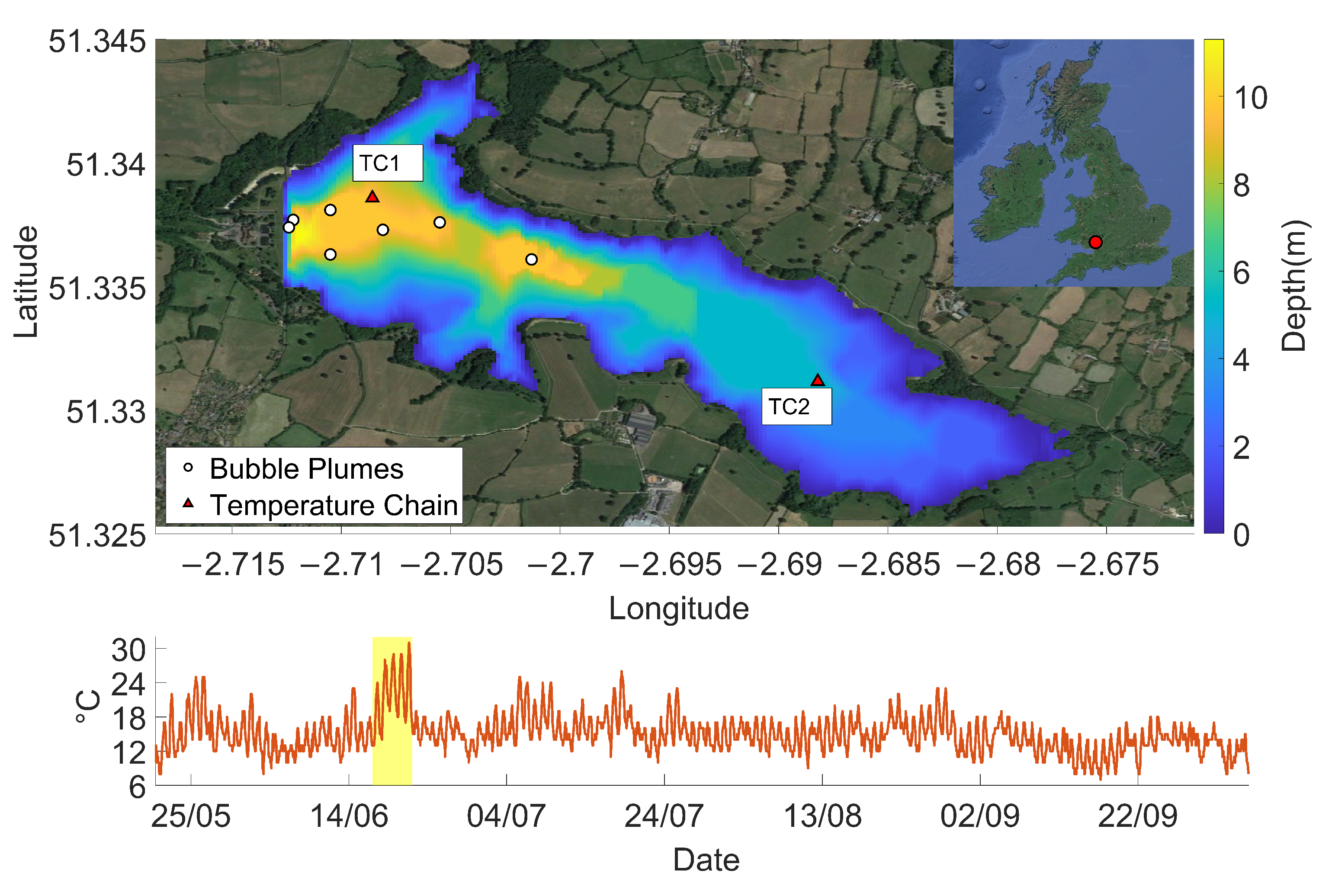
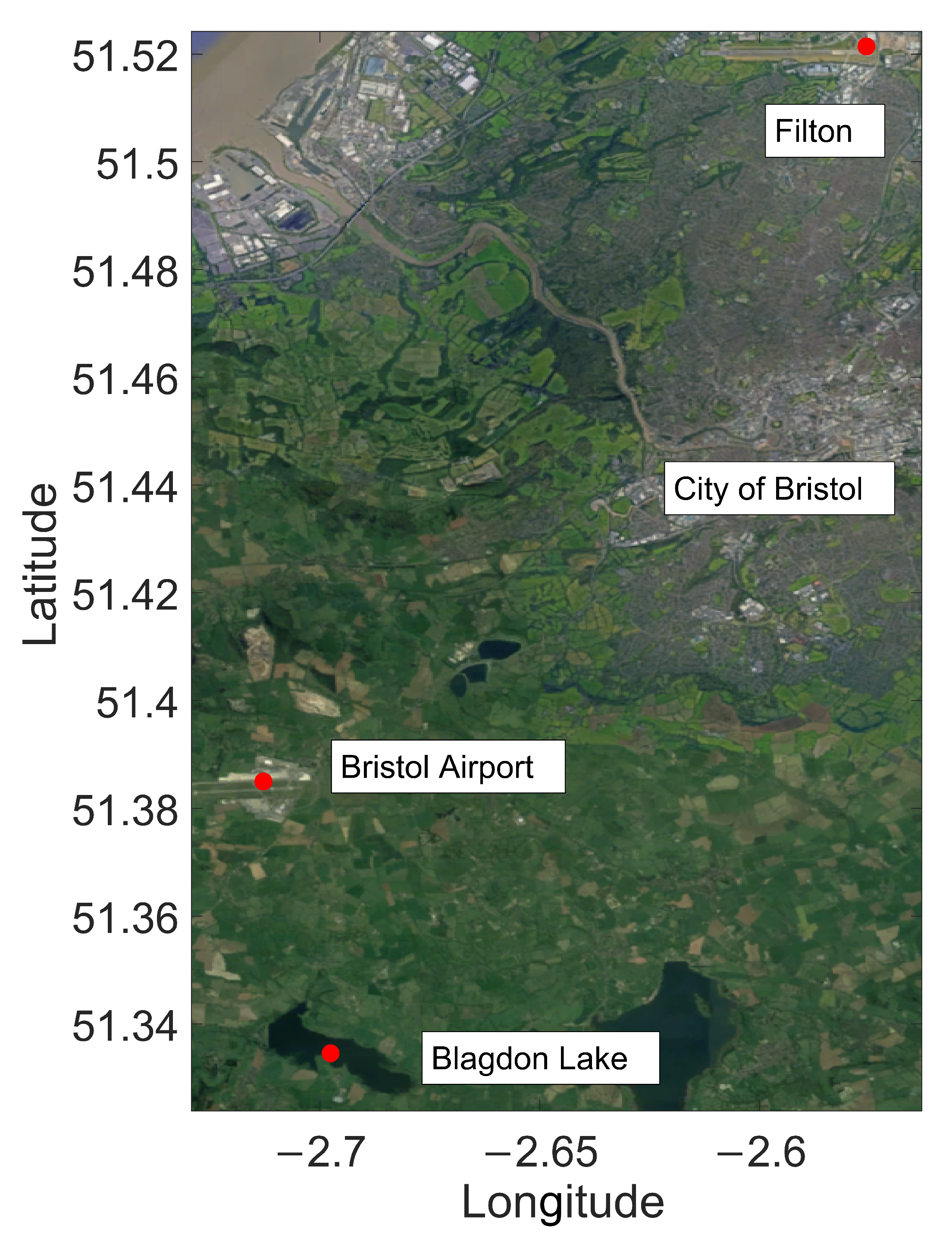
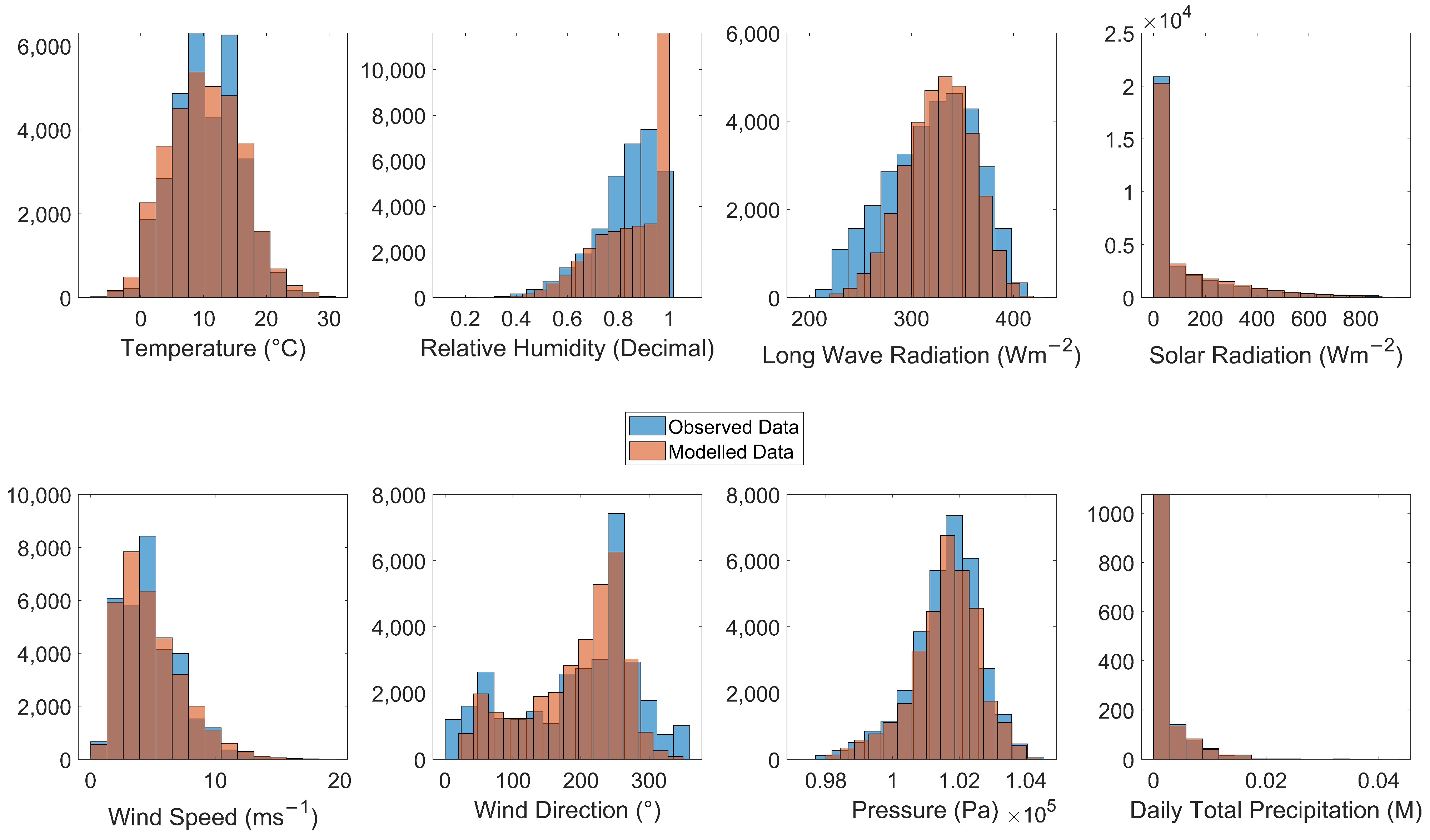
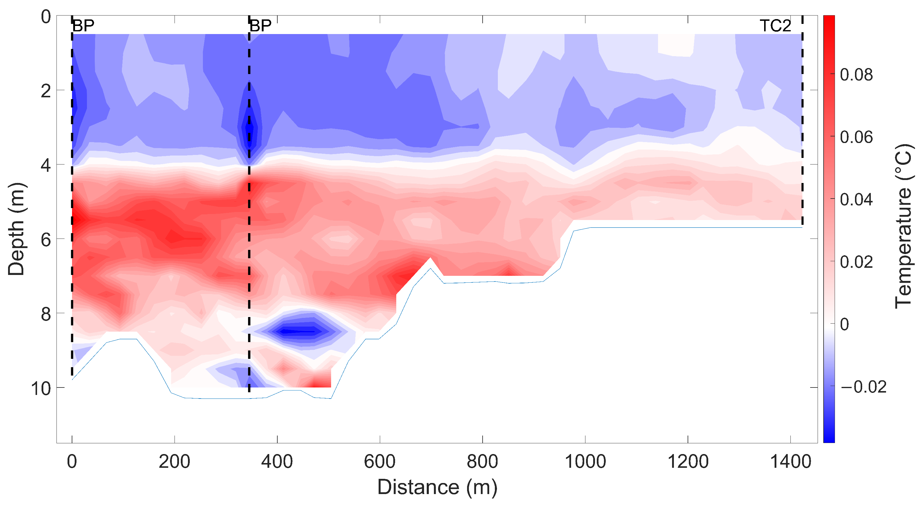
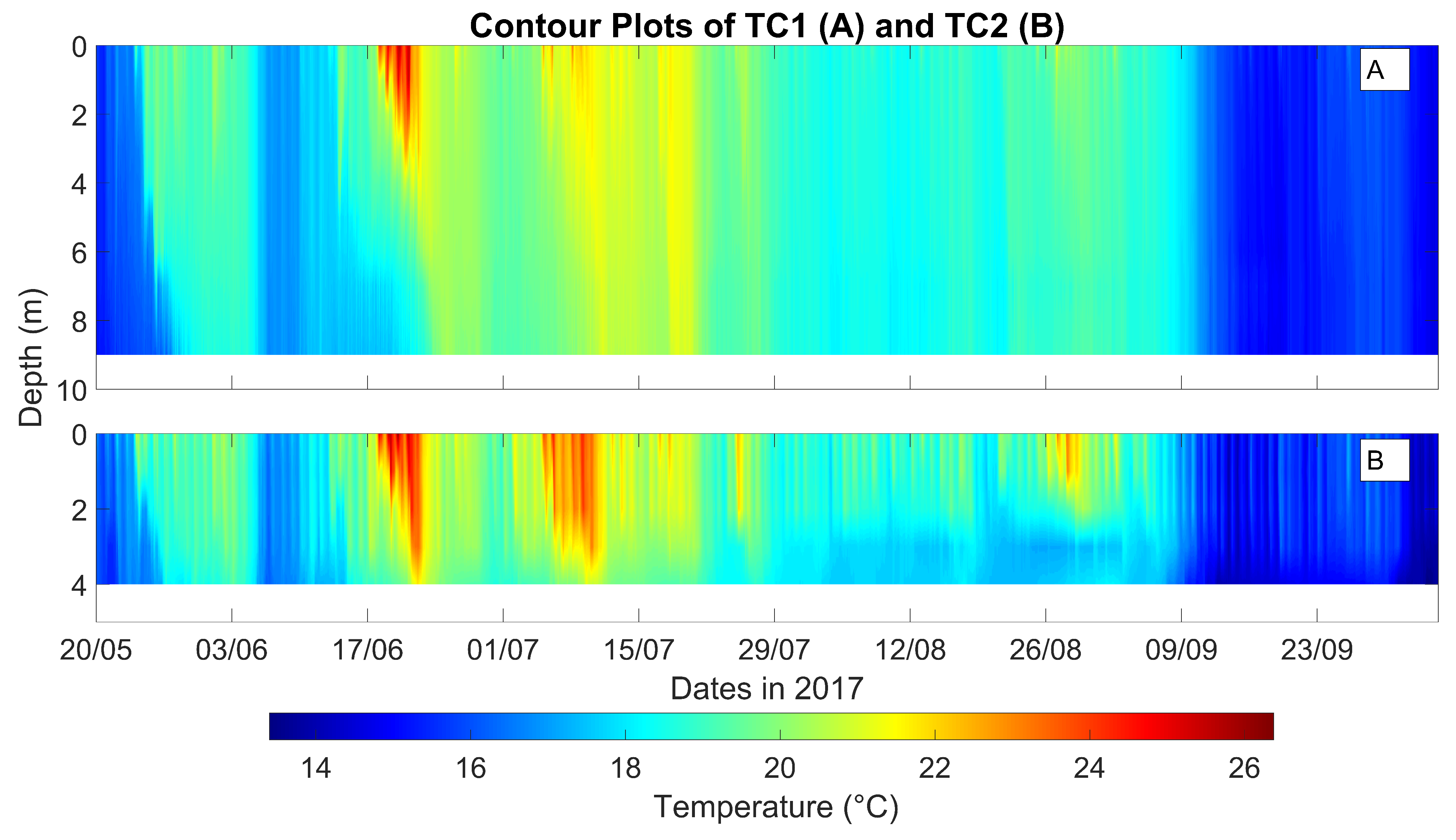
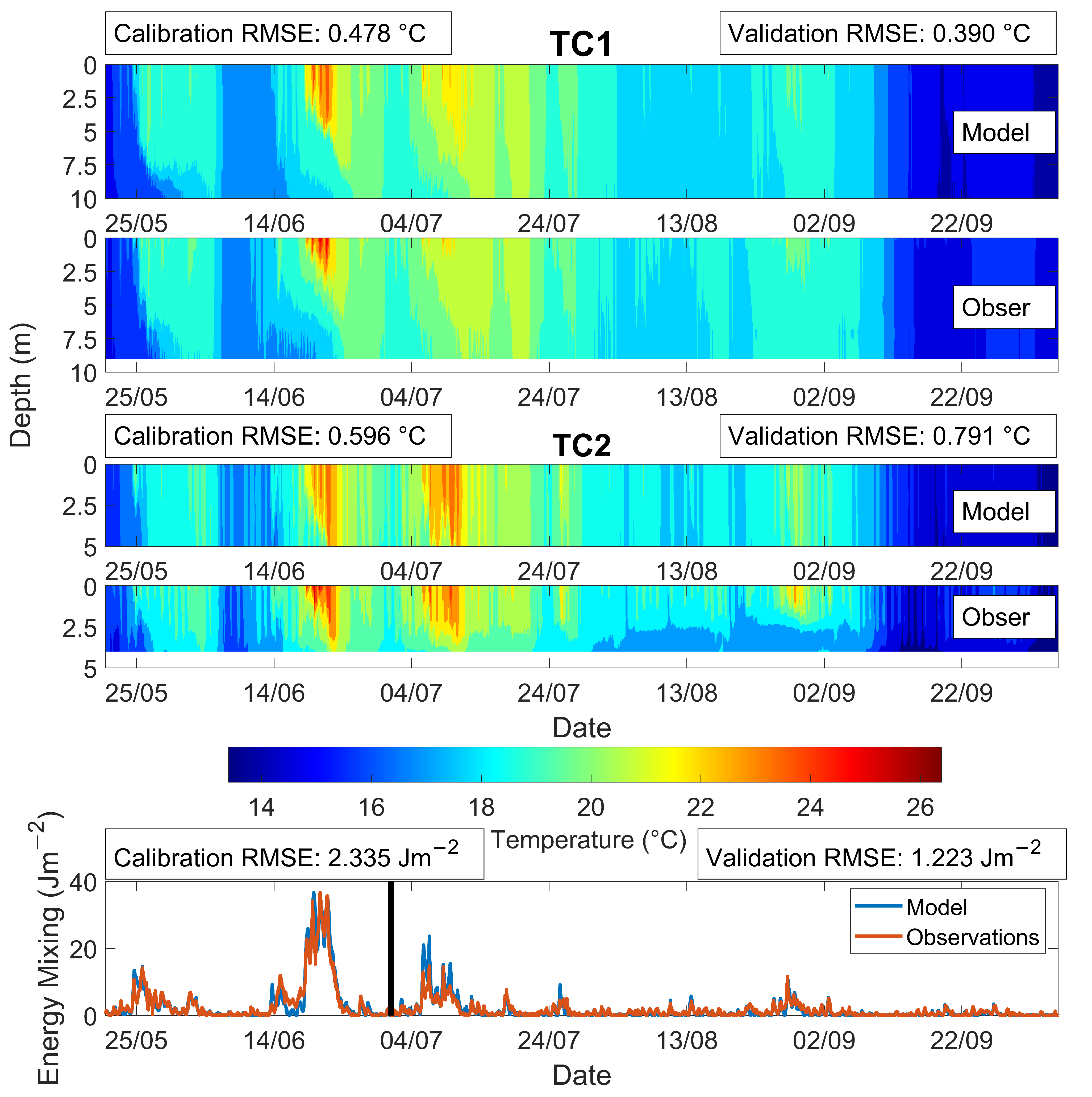
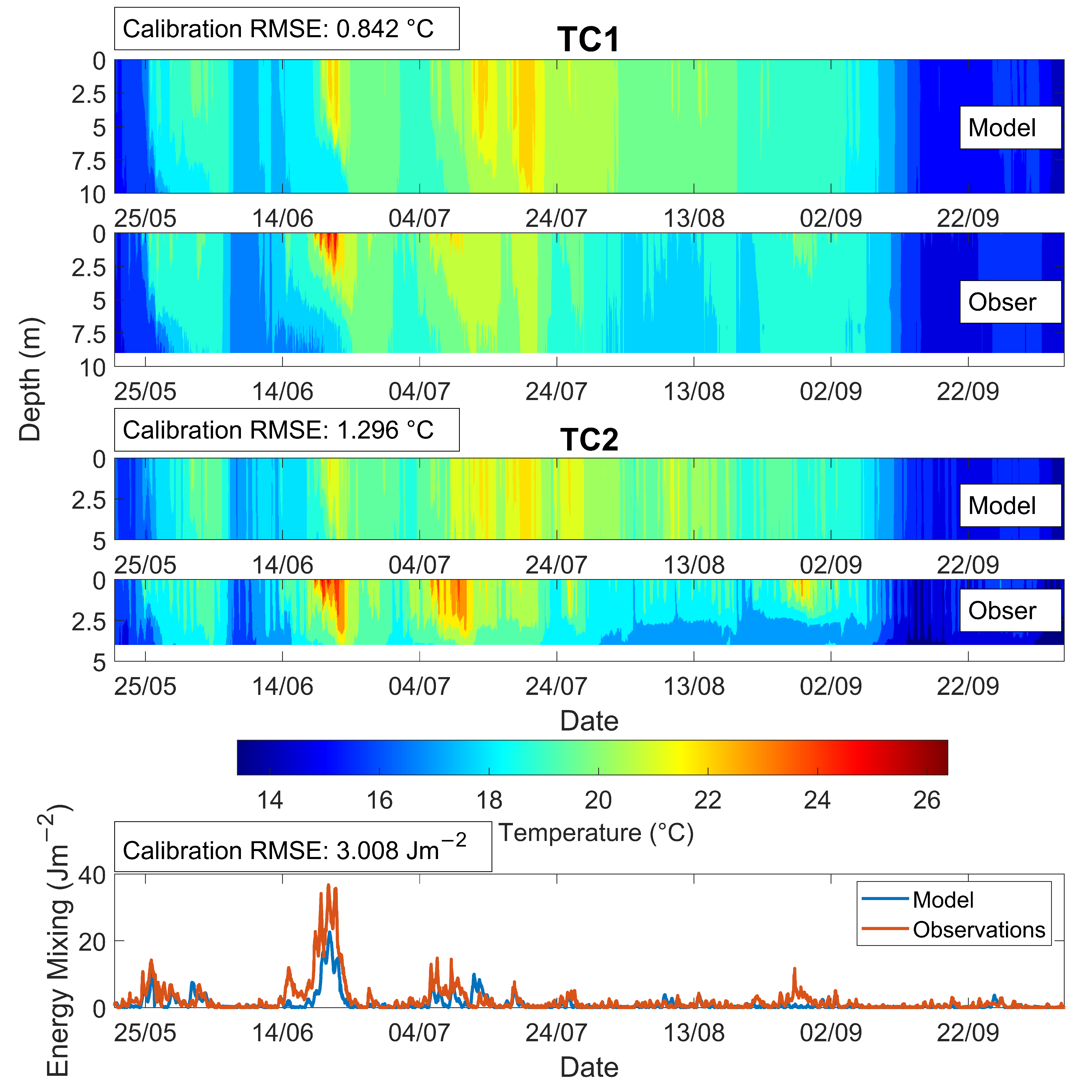
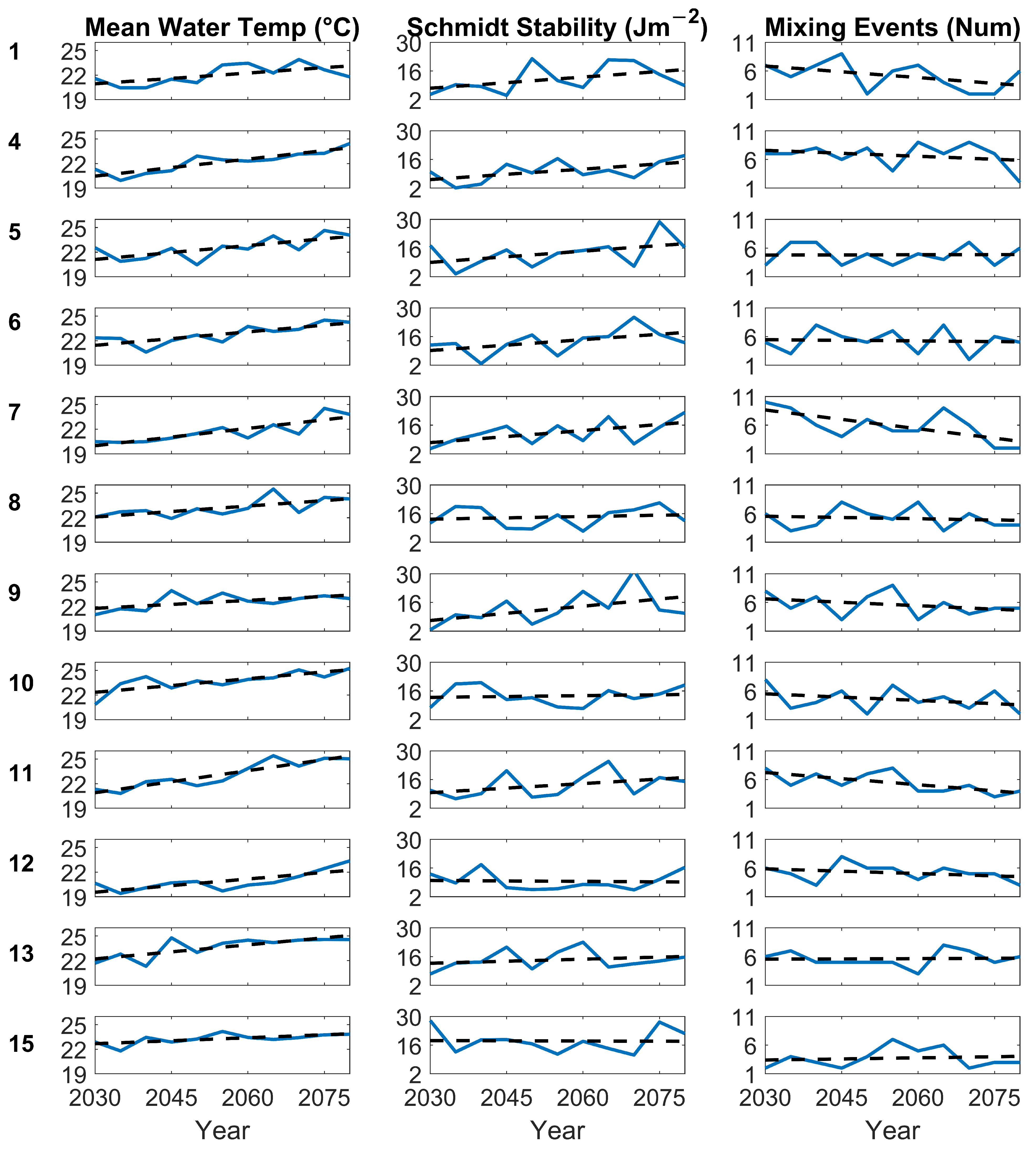
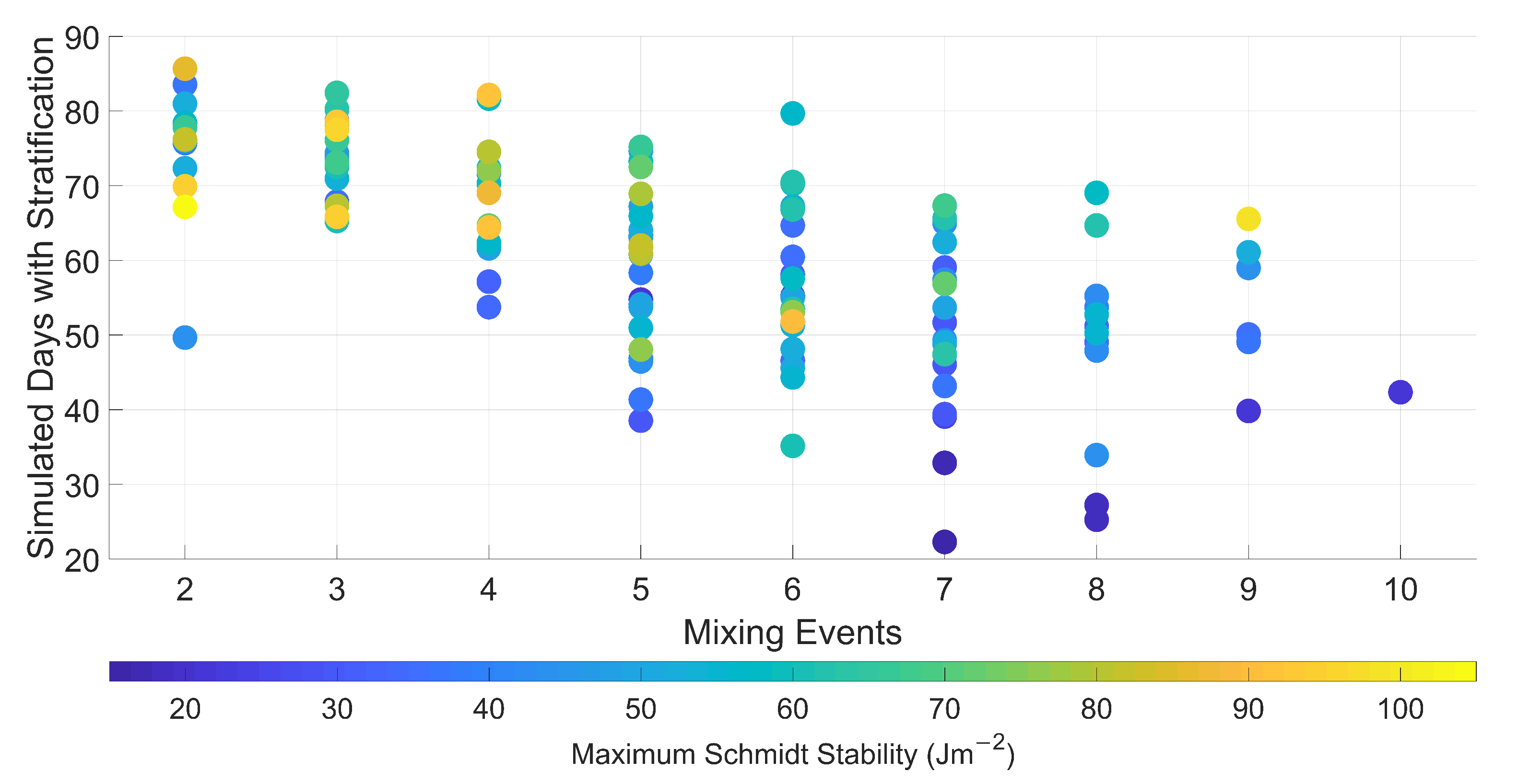
Table 1.
Root mean squared error (RMSE) and the Correlation Coefficients for comparison between the weather monitoring data and the down-scaled hourly data.
Table 1.
Root mean squared error (RMSE) and the Correlation Coefficients for comparison between the weather monitoring data and the down-scaled hourly data.
| Meteorological Factor | RMSE | Correlation Coefficient |
|---|---|---|
| Air Temperature | 1.6 (°C) | 0.96 |
| Relative Humidity | 0.09 (decimal) | 0.78 |
| Long-Wave Radiation | 26.87 (Wm) | 0.8 |
| Solar Radiation | 53.54 (Wm) | 0.95 |
| Wind Speed | 2.06 (ms) | 0.66 |
| Wind Direction | 55.23 (°) | 0.79 |
| Atmospheric Pressure | 253.52 (Pa) | 0.97 |
| Daily Total Precipitation | 0 (m) | 1 |
Table 2.
p-values (calculated with the Mann-Kendall test) and slope of fitted linear trend for mean water temperature, S and mixing events from the 12 different climate scenarios across the range of years the model was run for. Bold text shows statistically significant p-values of below 0.05, indicating a relationship between the modelled parameters and time not likely attributed to chance.
| Scenario | Mean Water Temperature (p-Values) | Schmidt Stability (p-Values) | Mixing Events (p-Values) |
| 1 | 0.062 | 0.350 | 0.186 |
| 4 | 0.002 | 0.119 | 0.876 |
| 5 | 0.087 | 0.276 | 1.000 |
| 6 | 0.020 | 0.062 | 0.876 |
| 7 | 0.003 | 0.119 | 0.043 |
| 8 | 0.043 | 0.876 | 0.755 |
| 9 | 0.087 | 0.119 | 0.392 |
| 10 | 0.008 | 0.755 | 0.436 |
| 11 | 0.003 | 0.350 | 0.043 |
| 12 | 0.008 | 0.755 | 0.276 |
| 13 | 0.013 | 0.276 | 1.000 |
| 15 | 0.062 | 0.755 | 0.697 |
| Scenario | Mean Water Temperature (Slope) | Schmidt Stability (Slope) | Mixing Events (Slope) |
| 1 | 0.044 | 0.182 | −0.067 |
| 4 | 0.069 | 0.170 | −0.035 |
| 5 | 0.056 | 0.183 | 0.002 |
| 6 | 0.055 | 0.177 | −0.007 |
| 7 | 0.070 | 0.197 | −0.109 |
| 8 | 0.045 | 0.043 | −0.015 |
| 9 | 0.032 | 0.232 | −0.040 |
| 10 | 0.055 | 0.028 | −0.038 |
| 11 | 0.090 | 0.147 | −0.071 |
| 12 | 0.054 | −0.016 | −0.027 |
| 13 | 0.057 | 0.066 | 0.004 |
| 15 | 0.024 | −0.006 | 0.013 |
Table 3.
p-values (calculated with the Mann-Kendall test) and slope of fitted linear trends for mean water temperature, S and mixing events from the 12 different climate scenarios across the range of years for which the model was run. Bold text shows statistically significant p-values of below 0.05, indicating a relationship between the modelled parameters and time not likely attributed to chance.
| Scenario | Period of Stratification (p-Values) | Extent of Stratification (p-Values) |
| 1 | 0.043 | 0.087 |
| 4 | 0.062 | 0.213 |
| 5 | 0.755 | 0.533 |
| 6 | 0.043 | 0.020 |
| 7 | 0.087 | 0.119 |
| 8 | 0.640 | 0.755 |
| 9 | 0.119 | 0.276 |
| 10 | 0.436 | 0.640 |
| 11 | 0.043 | 0.043 |
| 12 | 0.640 | 0.755 |
| 13 | 0.119 | 0.087 |
| 15 | 1.000 | 0.640 |
| Scenario | Period of Stratification (Slope) | Extent of Stratification (Slope) |
| 1 | 0.480 | 0.199 |
| 4 | 0.602 | 0.194 |
| 5 | 0.253 | 0.139 |
| 6 | 0.672 | 0.286 |
| 7 | 0.495 | 0.179 |
| 8 | 0.071 | 0.053 |
| 9 | 0.470 | 0.228 |
| 10 | 0.288 | 0.087 |
| 11 | 0.429 | 0.228 |
| 12 | 0.184 | 0.012 |
| 13 | 0.352 | 0.173 |
| 15 | −0.058 | −0.017 |
Publisher’s Note: MDPI stays neutral with regard to jurisdictional claims in published maps and institutional affiliations. |
© 2021 by the authors. Licensee MDPI, Basel, Switzerland. This article is an open access article distributed under the terms and conditions of the Creative Commons Attribution (CC BY) license (https://creativecommons.org/licenses/by/4.0/).
Share and Cite
MDPI and ACS Style
Birt, D.; Wain, D.; Slavin, E.; Zang, J.; Luckwell, R.; Bryant, L.D. Stratification in a Reservoir Mixed by Bubble Plumes under Future Climate Scenarios. Water 2021, 13, 2467. https://doi.org/10.3390/w13182467
AMA Style
Birt D, Wain D, Slavin E, Zang J, Luckwell R, Bryant LD. Stratification in a Reservoir Mixed by Bubble Plumes under Future Climate Scenarios. Water. 2021; 13(18):2467. https://doi.org/10.3390/w13182467
Chicago/Turabian StyleBirt, David, Danielle Wain, Emily Slavin, Jun Zang, Robert Luckwell, and Lee D. Bryant. 2021. "Stratification in a Reservoir Mixed by Bubble Plumes under Future Climate Scenarios" Water 13, no. 18: 2467. https://doi.org/10.3390/w13182467
Note that from the first issue of 2016, this journal uses article numbers instead of page numbers. See further details here.