Field Study on Wood Accumulation at a Bridge Pier

Abstract

Transported large wood (LW) in rivers may block at river infrastructures such as bridge piers and pose an additional flood hazard. An improved process understanding of LW accumulations at bridge piers is essential for a flood risk assessment. Therefore, we conducted a field study at the River Glatt in Zurich (Switzerland) to analyze the LW accumulation process of single logs at a circular bridge pier and to evaluate the results of previous flume experiments with respect to potential scale effects. The field test demonstrated that the LW accumulation process can be described by an impact, rotation, and separation phase. The LW accumulation was described by combining two simplified equilibria of acting forces and moments, which are mainly a function of the pier diameter, pier roughness, and flow properties. We applied the resulting analytic criterion to the field data and demonstrated that the criterion can explain the behavior of 82% of the logs. In general, the field observations confirmed previous results on the LW accumulation probability in the laboratory, which supports the applicability of laboratory studies to investigate LW–structure interactions.

1. Introduction

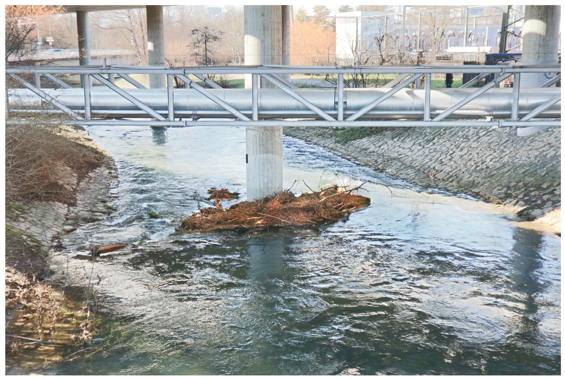
In forested river catchments, large wood (LW) may be entrained into the river due to landslides, bank failure, snow avalanches, or other erosion processes [1]. LW is defined as logs with a length ≥ $1.0$ m and diameter ≥ $0.1$ m [2]. During floods, the amount of transported LW can exceed the transport capacity of a river section and pose an additional flood hazard [1,3,4]. Specifically, LW may block at river infrastructures such as bridge piers (Figure 1), leading to increased water levels and potential flooding, or structural risks. The analysis of LW transport and accumulation processes, including the accumulation probability of LW at bridge piers, is key to improve the flood hazard assessment. The LW accumulation process has been investigated for different bridge types ranging from bridge decks to individual bridge piers [5,6,7,8,9,10,11,12,13,14,15,16,17,18].

Focusing on bridge piers, the accumulation process of logjams has been described by Panici and Almeida [12] to consist of three phases: unstable, stable, and critical. Using physical model tests, they observed that a logjam grows until a critical stage is reached and the logjam then separates from the pier and is transported downstream. According to field tests by Lyn et al. [6] and physical model tests by Panici and Almeida [12], logjams at bridge piers were more stable at lower flow velocities. The accumulation process of individual logs (i.e., uncongested LW transport according to Braudrick et al. [19]) at bridge piers has been investigated by Schalko et al. [20] for varying log geometries, pier characteristics, and flow conditions. During their physical model tests, they observed that logs rotated along the circular bridge pier and tended to resolve from the pier after reaching a critical log position angle. This angle can be determined based on a simplified force balance assuming that logs stay accumulated at a bridge pier given the acting hydraulic drag force is smaller or equal to the reactive force, which is described by the friction force between the log and the pier.

The majority of recent studies on the LW accumulation process at bridge piers were conducted using physical model tests with a model scale factor in the range of $\lambda =10$ to 50 under Froude similitude. Thus, the resulting pier (subscript p) and log (subscript L) Reynolds numbers, ${\mathsf{R}}_p=u{d}_p/\nu$ and ${\mathsf{R}}_L=u{L}_L/\nu$ with flow velocity u, pier diameter $d_p$, log length $L_L$, and kinematic viscosity $\nu$ are in a different flow regime compared to prototype conditions. This results in lower drag coefficients and affects the separation point and the wake area in prototype [20]. In addition, the strength characteristics and the Young’s modulus of the model logs may be overestimated as LW was modeled with wooden dowels [20]. In prototype, transported logs may break or bend when hitting a pier, thereby affecting the resulting LW accumulation process.

The limitations of physical model tests with respect to modeling LW and the flow structures in the vicinity of the pier can have implications on the LW accumulation process at bridge piers, affecting the resulting accumulation probability and the flood hazard assessment. Therefore, we conducted field experiments at the River Glatt in Zurich, Switzerland to validate the experimental results described in Schalko [16] and Schalko et al. [20] and to ensure their applicability under prototype conditions. This paper aims to improve the process understanding of the LW accumulation process at bridge piers, extend the introduced force balance [20] to describe why logs accumulate at bridge piers, and discuss potential model scale limitations.

2. Methods

2.1. Test Site

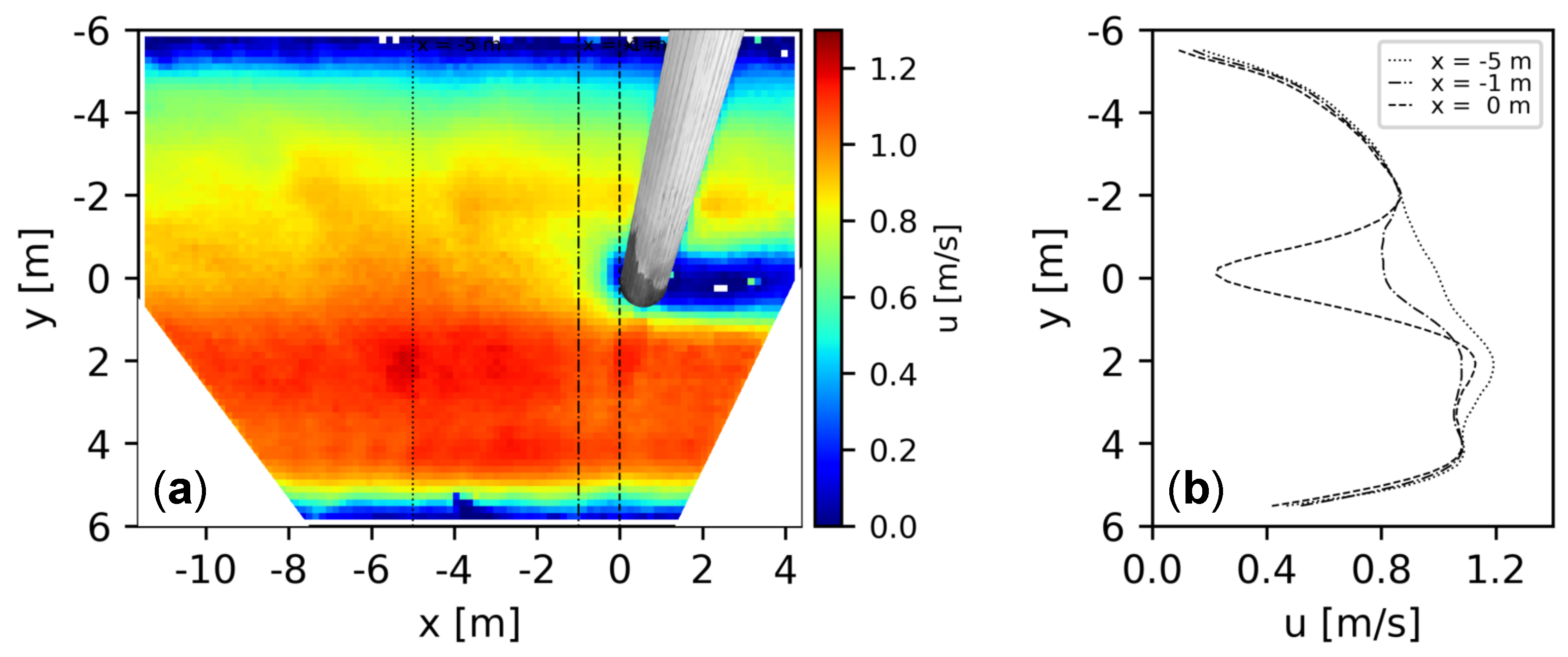
The field test was performed at the River Glatt in the city of Zurich, Switzerland (47.41137 N, 8.57198 E). The River Glatt is a tributary of the High Rhine and originates in the Lake Greifensee. It has a total length of 36 km, an average bed slope of 3‰, and a catchment area of 417 km². Its mean (subscript m) discharge at the test site is $Q_m=$ 4.4 ${\mathrm{m}}^3/\mathrm{s}$ [21]. The test site (Figure 2a) is situated 8 km downstream of the Lake Greifensee. A circular concrete bridge pier is located in the river centerline with a diameter of $d_p=1.2$ m. The River Glatt has fixed banks at the test site and a mobile bed. It is characterized by a channelized geometry with a river width of 12 m. During the field test, the flow conditions remained relatively constant with a discharge $Q=8.4 {\mathrm{m}}^3/\mathrm{s}$ in the morning and $Q=8.0 {\mathrm{m}}^3/\mathrm{s}$ in the afternoon. For $Q=8.0 {\mathrm{m}}^3/\mathrm{s}$, a mean surface flow velocity of $u_m=0.88 \mathrm{m}/\mathrm{s}$ and a mean water depth of $h_m=0.73 \mathrm{m}$ were measured 5 m upstream of the bridge pier ($x=-5\mathrm{m}$). These values correspond to an approach flow Froude number of $\mathsf{F}=u_m/\left(g{h}_m\right)=0.3$ with the gravitational acceleration g. Nonuniform flow conditions are present due to a slight left river bend. The surface velocity plot in Figure 3 illustrates that the streamwise surface velocities at the bridge cross section are 43% higher towards the right bank than towards the left bank ($u_{m,left}=0.72 \mathrm{m}/\mathrm{s}$ and $u_{m,right}=1.03 \mathrm{m}/\mathrm{s}$ at $x=0$ m).

2.2. Large Wood

A total of $n=55$ natural wooden logs (Picea abies) were added to the River Glatt and recorded by a camera for further evaluation. The logs were characterized by some irregularities in shape (Figure 2b) and had a mean log length of $L_L=4.0 \mathrm{m}\left(\pm 0.4 \mathrm{m}\right)$, a mean log diameter of $d_L=0.20 \mathrm{m}\left(\pm 0.05 \mathrm{m}\right)$, and a mean log density of ${\rho }_L=560\mathrm{kg}/ {\mathrm{m}}^3\left(\pm 110\mathrm{kg}/{\mathrm{m}}^3\right)$ (

Table 1. Mean, standard deviation, and extreme values of log length $L_L$, log diameter $d_L$, and log density ${\rho }_L$ of all tested logs ($n=55$).

	Mean	Std. Dev.	Minimum	Maximum
$L_L$ [m]	4.0	0.4	3.0	5.5
$d_L$ [m]	0.20	0.05	0.12	0.42
${\rho }_L$ [kg/m3]	560	110	320	750

).

2.3. Test Procedure

The field test was performed similar to the model tests by Schalko et al. [20] to evaluate the results. Single logs were added to the river 5 to 10 m upstream of the bridge pier using a truck crane (Figure 2a). To study the maximum accumulation probability [20], each log was added in such a way that it hit the bridge pier preferably centrically (eccentricity at impact $e_{imp}=0 \mathrm{m}$) and perpendicular to the main flow direction (yaw $\phi =0{}^{\circ }$). As soon as a log hit the pier, the duration until the log separated from the pier was measured and defined as the accumulation time $t_{acc}$. Logs that remained attached at the pier for $t_{acc}\ge 2 \min$ (120 s) were counted as accumulated and then removed from the pier by the truck crane. Logs that remained attached for $t_{acc}<2 \min$ were counted as not accumulated. For additional analysis, the entire accumulation process was recorded on video using a camera mounted on a tripod at the right river bank.

2.4. Video Analysis

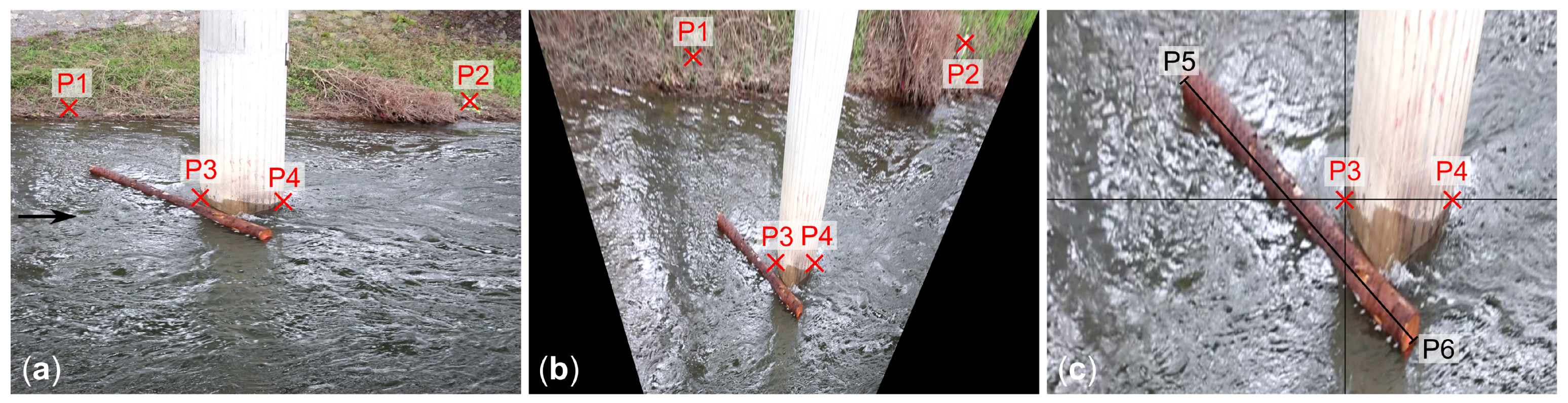
The analysis of $n=55$ videos included qualitative observations of the log movements at the pier as well as both manual and automatic detection of the log rotation. The manual detection was performed at the impact and separation points, which are defined as the points in time when a log hit the pier and separated from it, respectively. At each point, a snapshot was extracted from the video and the reference points P1 to P4 were manually detected (Figure 4a). Based on the perspective transformation of the snapshot (Figure 4b), which corrects the perspective distortion of the camera image, the log endpoints were determined (P5 and P6). Using points P4 to P6, the log orientation (eccentricity e and yaw $\phi$) was then calculated through trigonometry (Figure 4c).

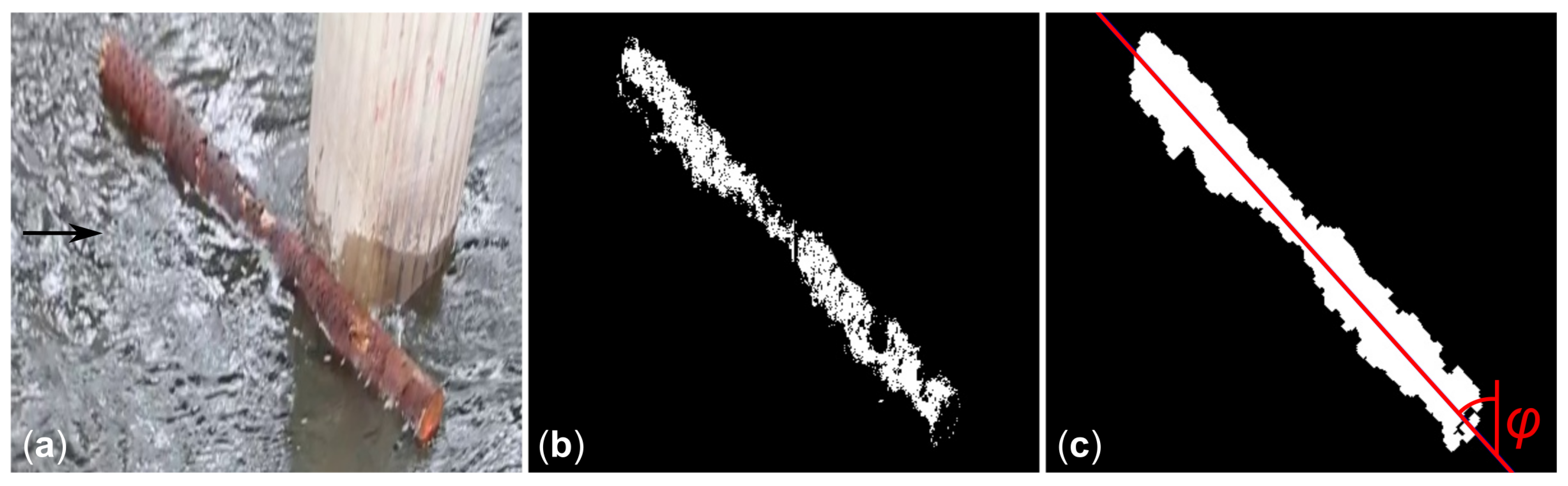
For selected logs, the log rotation was automatically detected. Snapshots were extracted from the video at a time interval of $\Delta t=0.24 {s}$ between the impact and separation points. This resulted in 500 snapshots per accumulated log (given $t_{acc}=120 {s}$). All extracted snapshots were perspectively transformed and cropped to a region of interest (Figure 5a). Within the region of interest, the log was detected using histogram backprojection (Figure 5b). This technique [22] allows to find regions of similar colors based on the color histograms of the object one is looking for and the image region one is searching in. The resulting image was dilated and a straight line was fitted to determine the yaw $\phi$ (i.e., its orientation relative to the main flow direction; Figure 5c).

Both the manual and automatic detection method rely on the perspective transformation of single frames. The perspective transformation was performed using two reference points at the left river bank (P1 and P2) and two reference points at the pier (P3 and P4). Whereas P1 and P2 are precisely defined by markers, P3 and P4 are less precisely defined (Figure 4a) and introduce an error of $\pm 5\%$ for lengths and $\pm 5{}^{\circ }$ for angles.

2.5. Surface Flow Field

The surface flow field around the bridge pier was measured using particle image velocimetry (PIV). Two reference PIV measurements were conducted without log addition (Figure 3) and two with a log accumulated at the bridge pier. During each measurement, a video ($1920\times 1080 {p}{{x}}^2$ at 25 fps) was recorded from a camera that was installed at the right bank of the river. A video clip of 30 s (750 frames) was then processed in two steps: First, the video frames were orthorectified on the basis of four ground reference points on the river banks, resulting in a raster scale of 100 px/m. Second, the mean surface velocities were determined using the MATLAB-based open source software PIVlab [23]. In the PIV-algorithm, a Fast Fourier Transformation window deformation was applied on a final grid of $32\times 32 {p}{{x}}^2$ with 50 overlap, which led to a spatial resolution of $0.16$ m. The error of the resulting mean surface velocities was estimated to be lower than $\pm 0.10 \mathrm{m}/\mathrm{s}$.

3. Results and Discussion

3.1. General Process Description

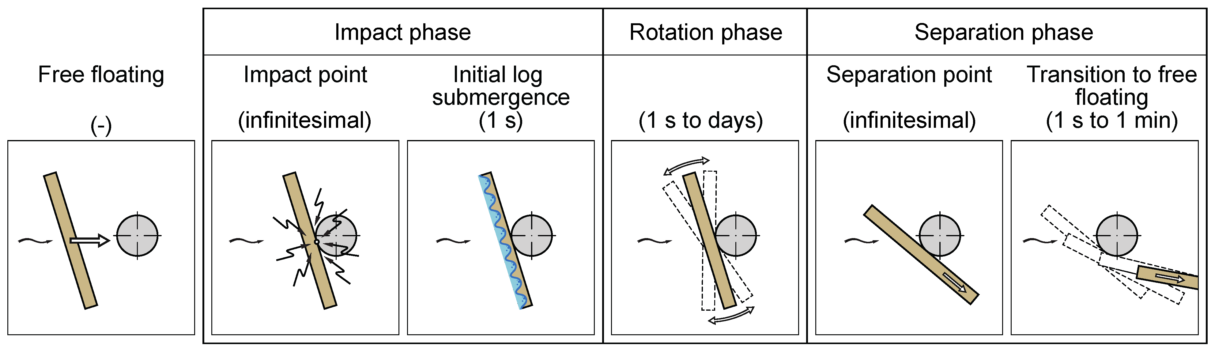
The accumulation process of a single log can be divided into the three characteristic phases of impact, rotation, and separation (Figure 6). These phases can vary in their distinctiveness depending on the shape of the log and its orientation during impact. For example, a log that hit the pier centrically exhibited a longer rotation phase than a log that hit the pier with a high eccentricity.

3.1.1. Impact Phase

The first phase of the accumulation process is the impact phase and covers the transition of a log from its free-floating state to its rotating state at the pier. It features two characteristic subprocesses: the impact point and the initial log submergence. As both subprocesses were quite short, the impact phase usually lasted for one to two seconds.

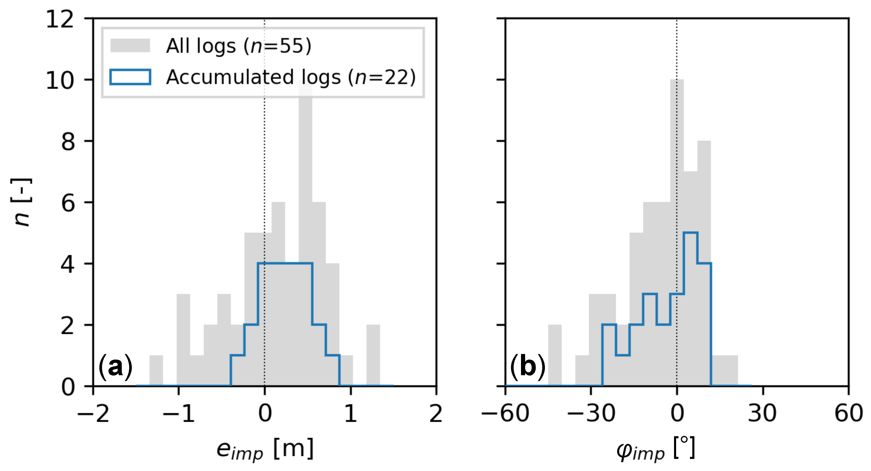
Impact point. The impact point was defined as the point in time when a free-floating log hit the pier. Figure 7 illustrates the observed log orientation at the impact point (subscript $imp$) by means of the eccentricity and yaw. The impact eccentricity $e_{imp}$ is defined as the distance between the log center and the contact point between log and pier along the log axis. Logs with a positive impact eccentricity $e_{imp}>0$ hit the pier with their center on the left side of the pier, and logs with a negative eccentricity $e_{imp}<0$ hit the pier with their center on the right side (in flow direction). The histogram of the impact eccentricity $e_{imp}$ (Figure 7a) shows a Gaussian-shaped distribution with most logs in the range of $e_{imp}=[-1.0,1.0]$ $\mathrm{m}$. Only a few logs hit the pier with a higher eccentricity. The highest observed eccentricities were $e_{imp}=\pm 1.3 \mathrm{m}$. The histogram of the impact yaw ${\phi }_{imp}$ (Figure 7b) illustrates a left skewed distribution with a maximum number of logs n at ${\phi }_{imp}=0{}^{\circ }$. Furthermore, Figure 7 shows that $n=22$ logs were only observed to accumulate given $e_{imp}=[-0.3,+0.8]$ $\mathrm{m}$ and ${\phi }_{imp}=[-25,+10]$ ${}^{\circ }$.

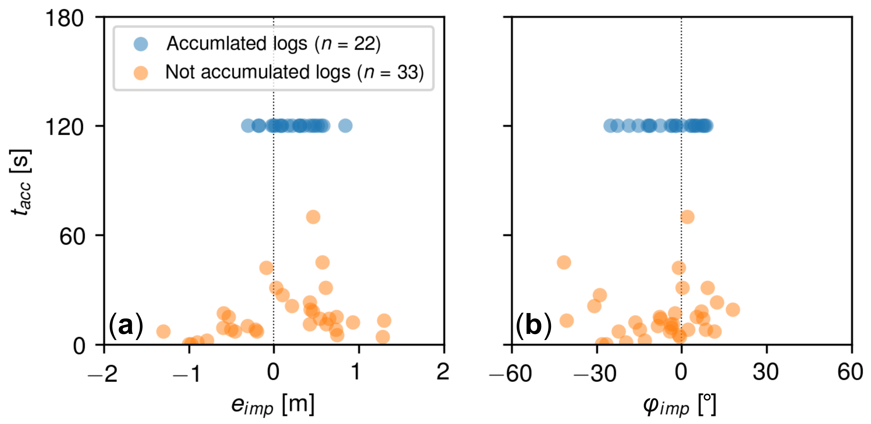
To study the effect of the log orientation in more detail, the accumulation time $t_{acc}$ was plotted versus the eccentricity $e_{imp}$ (Figure 8a) and the yaw ${\phi }_{imp}$ (Figure 8b), respectively. Figure 8a shows a clear dependency of $t_{acc}$ on $e_{imp}$, as logs with $e_{imp}=[-0.1,0.6]$ $\mathrm{m}$ were observed to remain attached for a longer period than logs with an eccentricity outside this interval. In contrast, the dependency of $t_{acc}$ on ${\phi }_{imp}$ is less clear (Figure 8b). Although the longest accumulation times were observed for logs with ${\phi }_{imp}=[0,10]$ ${}^{\circ }$, some logs with ${\phi }_{imp}=[-45,-30]$ ${}^{\circ }$ exhibit surprisingly long accumulation times (up to $t_{acc}=50 {s}$) as well, pointing at additional relevant processes that need to be considered.

Figure 8 further supports the introduced threshold time for the field test procedure. As stated in the methods section, logs that remained attached for longer than $t_{acc}\ge 120 {s}$ were defined as accumulated. Figure 8 now illustrates a clear gap between logs with accumulation times of $t_{acc}\le 70 {s}$ and $t_{acc}\ge 120 {s}$ indicating that logs separated before $t_{acc}=120 {s}$.

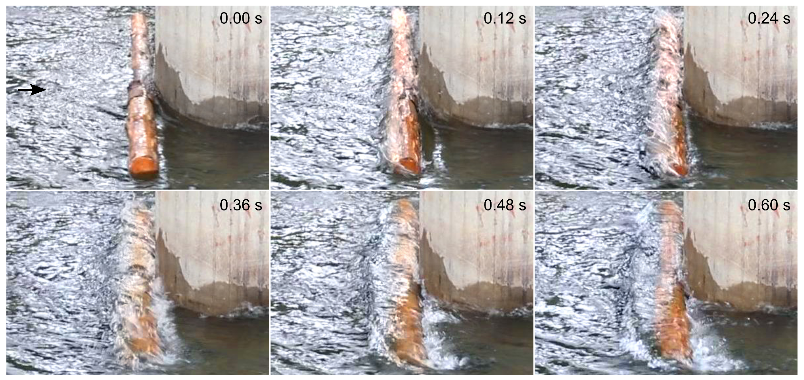
Initial log submergence. After the log impact on the pier, the log was observed to be pushed under water for a very short time duration of about one second. This subprocess is herein referred to as initial log submergence. Figure 9 shows a series of snapshots of a pronounced initial log submergence. The pictured log hit the pier quite concentrically with $e_{imp}=0.17 \mathrm{m}$ and perpendicular to the main flow direction with ${\phi }_{imp}=5{}^{\circ }$. As a result of the log’s impact on the pier (at time step $t=0.00 {s}$), a water wave was generated and spilled over the log ($t=0.12,0.24 {s}$). During the same time, the log changes its vertical position from an emergent position ($t=0.00 {s}$) to a partially submerged position ($t=0.36 {s}$ and later) with water flowing over it. This process was observed mainly for logs impacting centrically ($e_{imp}\approx 0 \mathrm{m}$). Logs impacting eccentrically ($e_{imp}>0.5 \mathrm{m}$) showed a less pronounced initial submergence.

We hypothesize that the initial log submergence is accompanied by sudden changes in the pressure distribution on the log. In its free-floating state, the log is subjected to a hydrostatic pressure distribution, which suddenly changes at the impact point. The water body upstream of the log is suddenly stopped, which leads to an increased pressure on the upstream side of the log, while the pressure decreases on the downstream side of the log. The increased pressure on the upstream side causes then the water to spill over the log. Impacting centrically ($e_{imp}\approx 0 \mathrm{m}$), a log stops a larger water body than impacting eccentrically (e.g., $e_{imp}>0.5 \mathrm{m}$), thus leading to a more pronounced initial submergence.

3.1.2. Rotation Phase

The rotation phase represents the second phase of the accumulation process (Figure 6). This phase begins just after the initial log submergence and lasts as long as the log keeps rotating around the pier. While some logs rotated fast around the pier and eventually separated from it, others rotated slowly to an equilibrium yaw and stayed attached (i.e., accumulated). Out of $n=55$ recorded logs, $n=22$ logs stayed attached to the pier for $t_{acc}\ge 120 {s}$ and were considered as accumulated logs, resulting in an accumulation probability of $p=22/55=0.40$, i.e., 40%. This value can be compared to the proposed design equation for p by Schalko et al. [20] using a normalized LW probability factor $L{W}_p$

$$\begin{array}{c}\hfill p=e^{-12.7L{W}_p}\end{array}$$

(1)

and

$$\begin{array}{c}\hfill L{W}_p=x_n{\left(\frac{u_o^2}{2g{L}_L}\right)}^{0.43}{\left(\frac{d_p}{L_L}\right)}^{0.60}\end{array}$$

(2)

with $x_n=1.00$ for uncongested LW transport and the approach flow velocity $u_o$. Applying Equations (1) and (2), $p=0.44$, i.e., 44% and agrees well with the observed accumulation probability of 40%, confirming the applicability of the design equation by Schalko et al. [20] under field conditions.

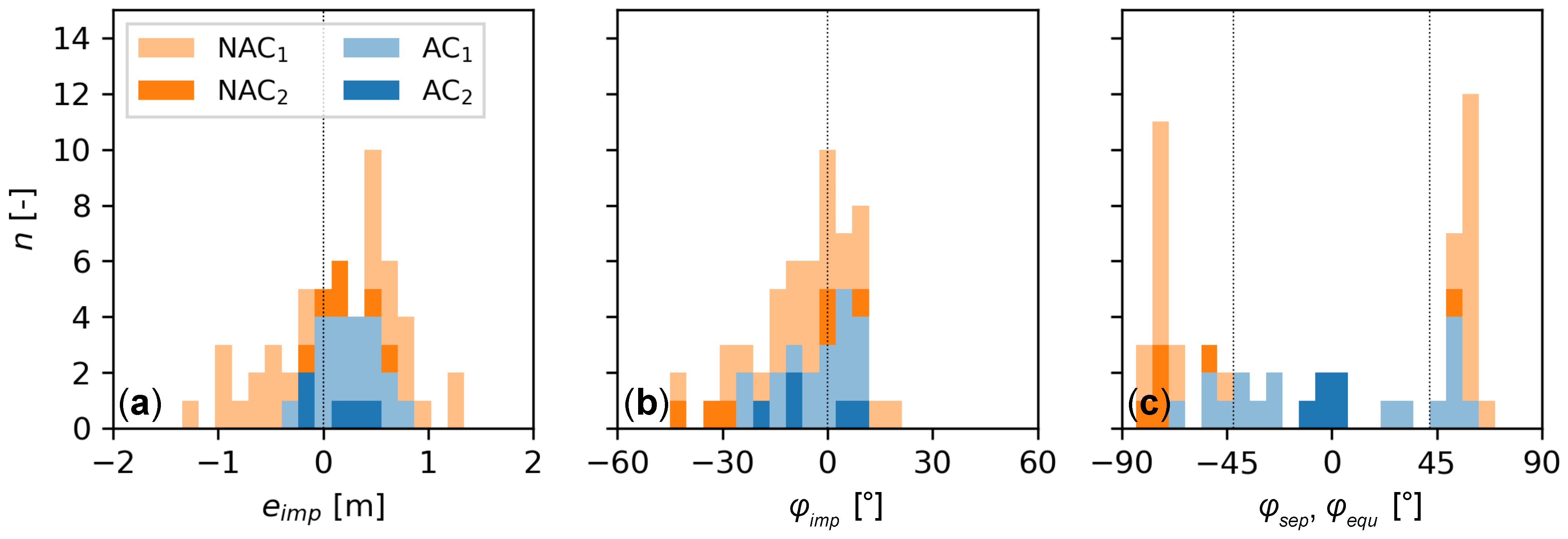
Log movement at the pier. During the rotation phase, different log movements were observed that allow to classify the logs in four classes: NAC₁, NAC₂, AC₁, and AC₂. While the two NAC-classes comprise all $n=33$ not accumulated logs, the two AC-classes comprise all $n=22$ accumulated logs (

Table 2. Observed movements of accumulated (AC₁, AC₂) and not accumulated logs (NAC₁, NAC₂) during rotation phase.

	Not Accumulated Logs		Accumulated Logs
Class	NAC1	NAC2	AC1	AC2
n[-]	27	6	17	5
Rotation	Fast, unidirectional	Slow, bidirectional	Slow, bidirectional	No
Oscillations	No	No	No	Yes
Submergence	in rare cases	in rare cases	partially	often completely
$|{\phi }_{sep}|$ [${}^{\circ }$]	$\left[45,80\right]$	$\left[50,80\right]$	-	-
$|{\phi }_{equ}|$ [${}^{\circ }$]	-	-	$\left[20,70\right]$	$\left[0,15\right]$
$t_{acc}$ [$\mathrm{s}$]	$\left[1,30\right]$	$\left[20,70\right]$	≥120	≥120

and Figure 10). A detailed list of the classified logs can be found in Appendix A.

For the not accumulated logs, 82% ($n=27$ out of 33) can be classified as NAC₁ logs. These logs were characterized by a fast and unidirectional rotation, i.e., they rotated around the pier in the horizontal plane without changing their direction of rotation. Due to their high rotation velocity, they separated after short accumulation times $t_{acc}=\left[1,30\right]$ $\mathrm{s}$. In contrast to the NAC₁ logs, NAC₂ logs showed a significantly slower rotation velocity and a bidirectional rotation, i.e., the logs changed their rotation direction at least once during the rotation phase. As this rotation behaviour was mainly observed for accumulated logs, it can be assumed that NAC₂ logs were close to being accumulated at the pier. This is also reflected in their rather long accumulation time of $t_{acc}=\left[50,80\right]$ $\mathrm{s}$.

For the accumulated logs, 77% ($n=17$ of 22) can be classified as AC₁ logs. These logs were characterized by a slow and bidirectional rotation. After their impact and initial submergence, they rotated from their impact yaw ${\phi }_{imp}$ towards an equilibrium (subscript $equ$) yaw in the range of $|{\phi }_{equ}|=\left[20,70\right]$ ${}^{\circ }$ (Figure 10c) and kept rotating around ${\phi }_{equ}$. However, $n=5$ accumulated logs showed a distinctively different behavior than the AC₁ logs and were classified as AC₂ logs. These logs impacted with $|{\phi }_{imp}|=\left[0,15\right]$ ${}^{\circ }$ and remained in an equilibrium yaw close to their impact yaw ${\phi }_{equ}\approx {\phi }_{imp}$. AC₂ logs often remained completely submerged after their initial submergence. Due to their submergence, they exhibited stronger hydraulic drag forces than AC₁ logs as well as oscillations at the pier, i.e., rotation in the vertical and horizontal direction with abrupt changes in rotation direction and velocity.

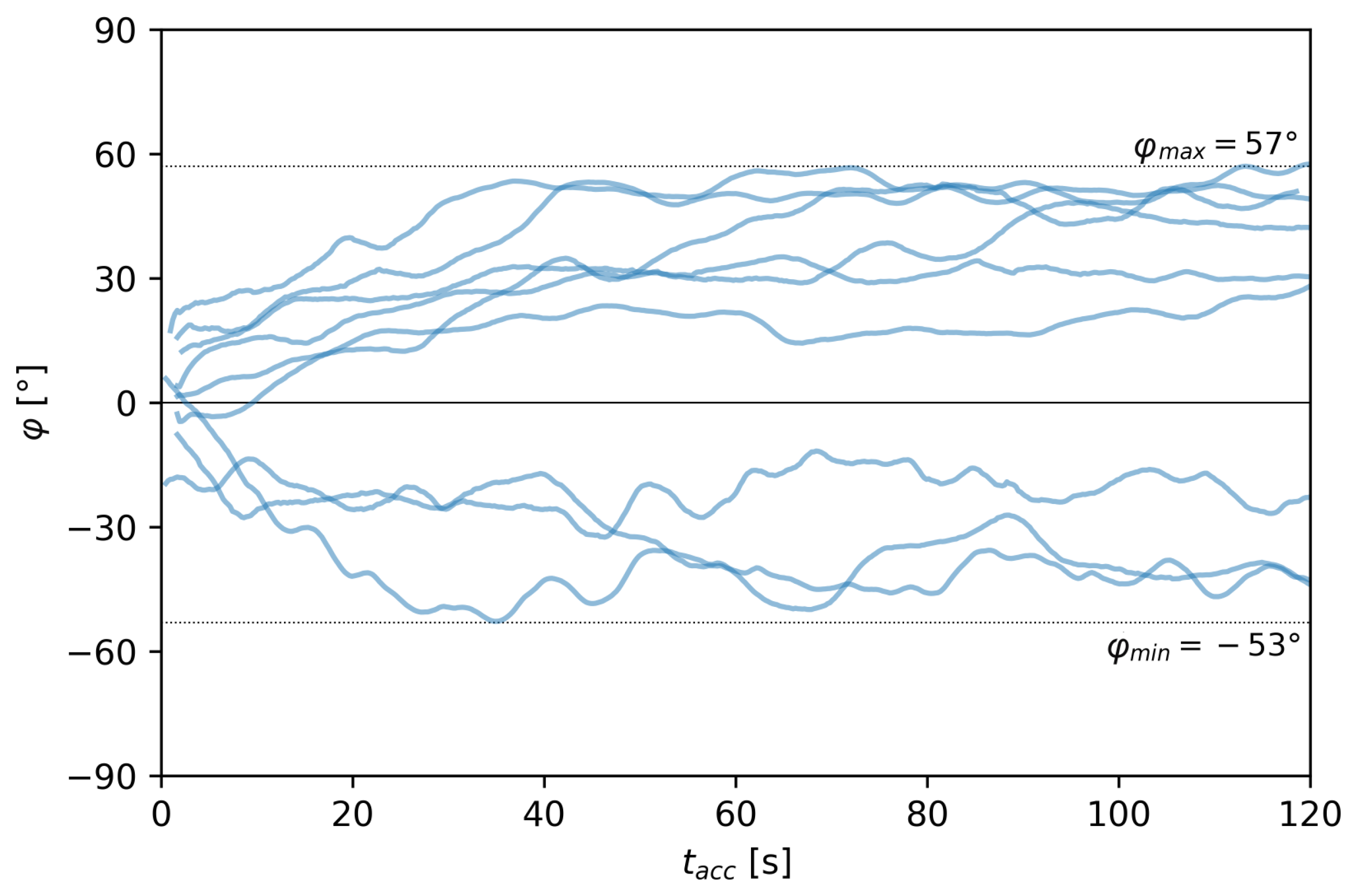
In Figure 11, the log rotation is illustrated for $n=9$ selected AC₁ logs. The logs impacted with ${\phi }_{imp}=\left[-20,20\right]$${}^{\circ }$ and subsequently rotated towards more extreme yaws with ${\phi }_{min}=-53{}^{\circ }$ and ${\phi }_{max}=57{}^{\circ }$. Most of the logs reached ${\phi }_{equ}$ after $t_{acc}=40\mathrm{s}$. They then kept rotating bidirectionally around ${\phi }_{equ}$ until the end of the observation period at $t_{acc}=120\mathrm{s}$.

To evaluate if the log rotation is influenced by the vortex shedding frequency at the cylindrical pier $f_p$, the frequency of the log rotation $f_L$ was analyzed for $t_{acc}=\left[40,120\right]$ $\mathrm{s}$ and compared to the literature. According to Achenbach and Heinecke [24] a Strouhal number of $\mathsf{S}=0.26$ can be assumed for a cylindrical pier with a Reynolds number of $\mathsf{R}=u_{o,m}{d}_p/\nu ={10}^6$, with the kinematic viscosity $\nu$ and a relative roughness coefficient $k_s/d_p=0.8\times {10}^{-3}$ ($k_s\approx 1\mathrm{mm}$). The vortex shedding frequency at the pier resulted in $f_p=u_{o,m}\mathsf{S}/d_p=0.19\mathrm{Hz}$ (with period $T_p=1/f_p=5.3 {s})$. However, the logs were observed to rotate with $f_L\approx \left[0.05,0.10\right]$ $\mathrm{Hz}$, not indicating a correlation between the log rotation frequency and the vortex shedding frequency of the pier.

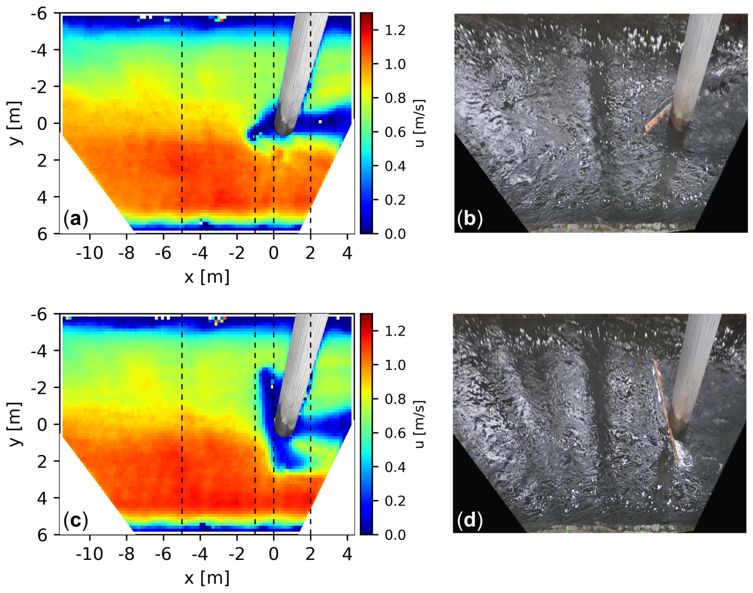
Log-induced changes in the flow field. A log accumulation at a bridge pier reduces the open flow cross section and will affect the flow conditions in the vicinity of the bridge pier. The surface flow field is illustrated in Figure 12 for two logs (log #7 and #22). The logs were accumulated at $\phi \approx 45{}^{\circ }$ (log #7) and $\phi \approx -15{}^{\circ }$ (log #22) and can be characterized as AC₁ and AC₂, respectively. Both logs led to small surface velocities in the range of $u=\left[0,0.2\right]$ $\mathrm{m}/\mathrm{s}$ directly up- and downstream of the log. The logs’ influence on the flow field is also reflected in the cross-sectional averaged velocity $\overline{u}$ (

Table 3. Cross-sectional averaged streamwise surface velocity $\overline{u}$ [$\mathrm{m}/\mathrm{s}$] for AC₁ and AC₂ logs shown in Figure 12. The reference without a log accumulated at the pier is shown in Figure 3.

	$\mathit{x}=-5\mathbf{m}$	$\mathit{x}=-1\mathbf{m}$	$\mathit{x}=0\mathbf{m}$	$\mathit{x}=2\mathbf{m}$
No log (reference)	0.88	0.81	0.73	0.77
Log #7 with $\phi \approx 45{}^{\circ }$	0.83	0.70 a	0.61 a	0.58
Log #22 with $\phi \approx 0{}^{\circ }$	0.86	0.77	0.47 a	0.54

^a Note that the log intersects with the cross-section.

). At the pier cross section ($x=0 \mathrm{m}$), both logs reduced the surface velocities compared to the reference flow field with no log accumulated at the bridge pier. Log #22 reduced $\overline{u}$ by 36% due to its orientation almost perpendicular to the main flow direction, thereby blocking a larger flow cross section. In comparison, log #7 reduced $\overline{u}$ by 16% with its yaw of $\phi \approx 45{}^{\circ }$. One meter upstream of the pier ($x=-1 \mathrm{m}$), the influence of log #22 was not present anymore (Figure 12c), while log #7 still showed a significantly reduced flow velocity 14% compared to the reference flow field. At $x=-5 \mathrm{m}$, the effect of a log accumulation on the surface flow field was not observed anymore. The log accumulation also affected the downstream flow conditions. Two meters downstream of the pier ($x=2 \mathrm{m}$), the surface velocities were reduced by 25% (log #7) and 30% (log #22), respectively, compared to the reference flow field. Based on Figure 12a,c in comparison to Figure 3, it can be assumed that the logs affected the flow conditions even further downstream.

3.1.3. Separation Phase

The separation phase represents the third phase of the accumulation process. It starts at the separation point, defined as the point in time, when the log movements indicated first signs of separation from the pier. The most common signs of separation were sliding-movements of the log on the pier, suggesting that the static friction force between log and pier is smaller than hydraulic force pushing the log downstream (Figure 13). Such sliding-movements were only present when the log was separating and not during the rotation phase, which simplified the identification of the separation point.

After the initiation of the separation phase, the log remained in contact with the pier for a few seconds. The log was still sliding on and rotating around the pier, and thus its movements were still influenced by the pier. Once the log has rotated far enough around the pier, it lost its contact with the pier and the transition to the free-floating state was completed.

To better understand why a log separated from the pier or not, the log orientation at the separation point was examined in more detail. Schalko [18] described a critical yaw angle ${\phi }_{cr}$ at which $F_{Friction}$ equals the parallel component of the hydraulic drag force $F_{\Vert }$, which pushes the log tangentially along the pier. For $\left|\phi \right|<{\phi }_{cr}$, $F_{Friction}$ is larger than $F_{\Vert }$ and the log remains accumulated. For $\left|\phi \right|>{\phi }_{cr}$, $F_{Friction}$ is smaller than $F_{\Vert }$ and the log separates. The critical yaw ${\phi }_{cr}$ depends solely on the static friction coefficient $\mu$ with ${\phi }_{cr}=\pm arctan\left(\mu \right)$, see detailed derivation in Section 3.2. Given a static friction coefficient for wood on concrete surfaces of $\mu =0.9$ [25], ${\phi }_{cr}=\pm 42{}^{\circ }$ can be expected for the field test. Logs with $-42{}^{\circ }\le \phi \le +42{}^{\circ }$ are expected to remain accumulated, while logs with $\left|\phi \right|>42{}^{\circ }$ are expected to separate from the pier. According to Figure 10c, the observed yaws for not accumulated logs at the separation point ${\phi }_{sep}$ were consistently greater than the critical value $|{\phi }_{sep}|>{\phi }_{cr}$, which is in agreement with the theory [18]. In addition, no separation of logs was observed for $\left|\phi \right|<{\phi }_{cr}$ (Figure 10c). However, some logs remained accumulated with $|{\phi }_{equ}|>{\phi }_{cr}$, where $F_{Friction}$ is supposed to be not sufficient to hold the log at the pier. This behavior was also observed in the flume experiments [18] and may be explained by local irregularities (e.g., bark, knotholes, or other geometrical irregularities) that favor the accumulation.

3.2. Formulation of a Static Accumulation Criterion

The observations suggest that the log orientation at the impact point influences whether a log remains accumulated or separates (Figure 10). To explain this relation, an analytic criterion was derived based on simplified equilibria of forces and moments.

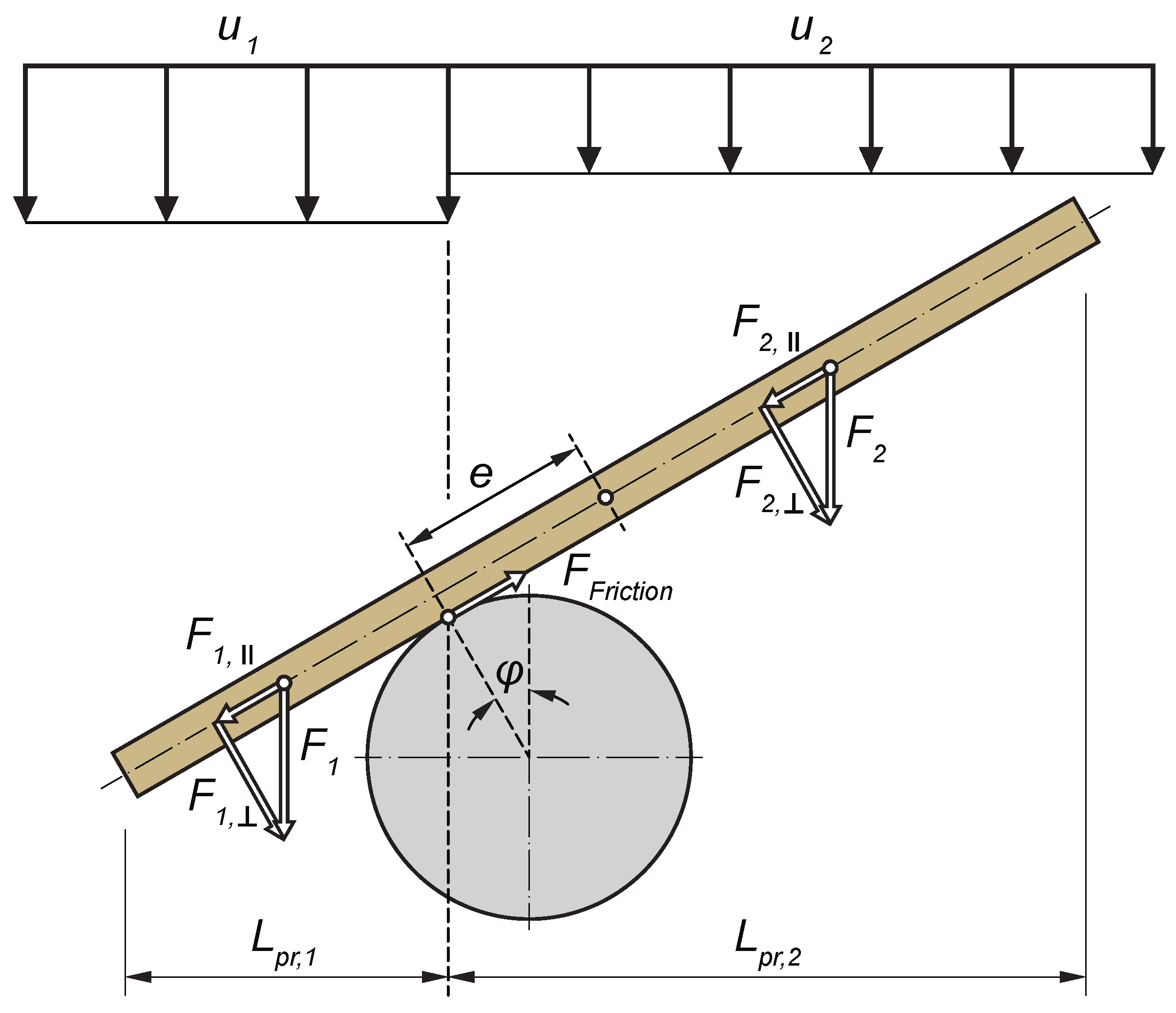
Definition of the acting forces. The accumulation criterion is based on a simple force system (Figure 13). This force system was first introduced by Schalko [18] for uniform flow velocities $u=u_1=u_2$ and herein adapted for nonuniform flow velocities with $u_1\ne u_2$, i.e., different flow velocities on the left and right side of the pier. The flow velocities $u_1$ and $u_2$ are defined as the mean average streamwise flow velocity at the pier cross section ($x=0$) at $y=[0,2]$ m for $u_1$ and at $y=[-2,0]$ m for $u_2$. Thus, a log with $L_L=4.0 \mathrm{m}$, $e_{imp}=$ 0 m, and ${\phi }_{imp}=$ 0° would experience $u_1$ and $u_2$. The flow velocities $u_i$ lead to different hydraulic drag forces on the respective part of the log, which can be defined as $F_i={\rho }_w{C}_d{A}_{pr,i}{u}_i^2/2$, with water density ${\rho }_w$, drag coefficient $C_d$, projected area $A_{pr,i}$, and subscript i denoting the respective part of the pier. A log remains accumulated as long as the parallel component of the total hydraulic drag force acting on the log $F_{\Vert }=F_{1,\Vert }+F_{2,\Vert }$ is smaller than the friction force between the log and the pier $F_{Friction}=\mu F_{\perp }$, with the static friction coefficient $\mu$ and the component of the total hydraulic drag force perpendicular to the log $F_{\perp }=F_{1,\perp }+F_{2,\perp }$ (Figure 13). Any other processes such as dynamic components of the system, turbulent fluctuations, or a changing flow field are neglected in this approach.

Equilibrium of forces. The equilibrium of forces is set up at the contact point between the log and the pier. At this point, $F_{Friction}$ must be equal to (or greater than) $F_{\Vert }$ to hold the log at the pier.

$$\begin{array}{c}\hfill F_{Friction}=F_{\Vert }\end{array}$$

(3)

with

$$\begin{array}{cc}\hfill F_{Friction}& =\mu cos\left|\phi \right|\left(F_1+F_2\right)\hfill \end{array}$$

(4)

$$\begin{array}{cc}\hfill F_{\Vert }& =sin\left|\phi \right|\left(F_1+F_2\right)\hfill \end{array}$$

(5)

By substituting Equations (4) and (5) into Equation (3), the critical yaw ${\phi }_{cr}$ can be determined for which $F_{Friction}$ is just large enough to compensate the hydraulic drag force $F_{\Vert }$

$$\begin{array}{c}\hfill {\phi }_{cr}=\pm arctan\mu \end{array}$$

(6)

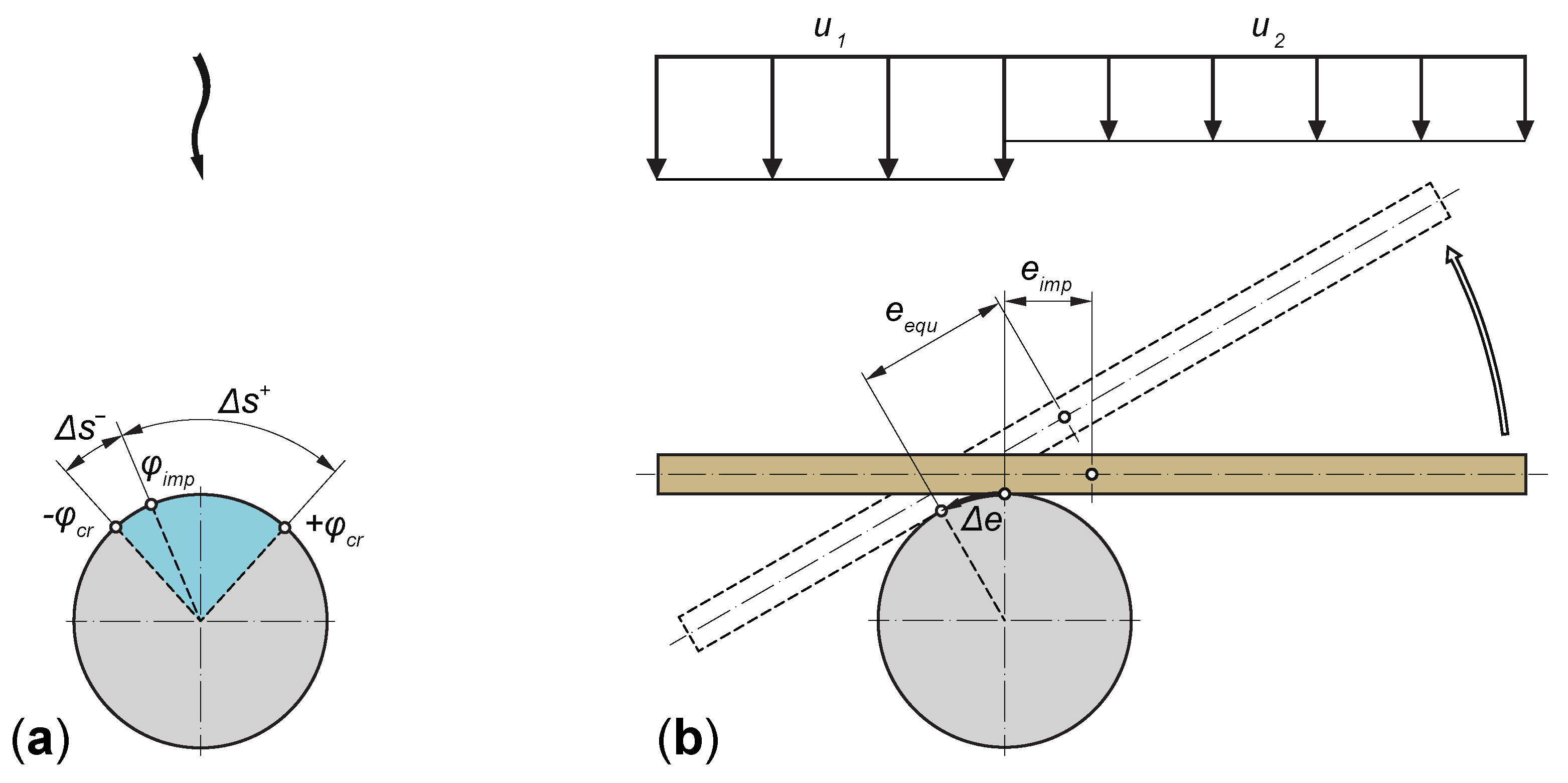
Thus, ${\phi }_{cr}$ is solely dependent on the static friction coefficient $\mu$ and results in ${\phi }_{cr}=\pm 42{}^{\circ }$ from $\mu =0.9$ (wood on concrete) [25]. However, the exact value of $\mu$ is uncertain and assumed to lie between 0.5 and 1.1 [26]. This results in ${\phi }_{cr}=\pm [27{}^{\circ },48{}^{\circ }]$. The resulting range $-{\phi }_{cr}<\phi <+{\phi }_{cr}$ is illustrated by the blue area in Figure 14a and describes where a log can accumulate at the pier. Figure 14a further shows how far a log can rotate at the pier before it must separate. If a log impacts with ${\phi }_{imp}$ it can rotate for $\Delta s^{-}=\pi d_p\left(-{\phi }_{cr}-{\phi }_{imp}\right)/360{}^{\circ }$ in the negative yaw direction or for $\Delta s^{+}=\pi d_p\left({\phi }_{cr}-{\phi }_{imp}\right)/360{}^{\circ }$ in the positive yaw direction. Thus, $\Delta s^{-}$ and $\Delta s^{+}$ represent the maximum available distances a log can rotate before it separates from the pier. The longer $\Delta s^{-}$ and $\Delta s^{+}$, the more likely will a log accumulate at the pier. As $\Delta s^{-}$ and $\Delta s^{+}$ are functions of $d_p$ and $\mu$, a log is more likely to accumulate if $d_p$ and $\mu$ are high. This relationship confirms the findings by Schalko [18].

Equilibrium of moments. The equilibrium of moments is also defined at the contact point between the log and the pier. The acting moments can be written as $|M_i|=\frac{1}{2}{L}_{pr,i}{F}_i$ and thus the equilibrium is

$$\begin{array}{c}\hfill \frac{1}{2}{L}_{pr,1}{F}_1=\frac{1}{2}{L}_{pr,2}{F}_2\end{array}$$

(7)

with

$$\begin{array}{cc}\hfill F_i& ={\rho }_w{C}_d{L}_{pr,i}{d}_L\frac{u_i^2}{2}\hfill \end{array}$$

(8)

$$\begin{array}{cc}\hfill L_{pr,1}& =(\frac{L_L}{2}-e)cos\phi \hfill \end{array}$$

(9)

$$\begin{array}{cc}\hfill L_{pr,2}& =(\frac{L_L}{2}+e)cos\phi \hfill \end{array}$$

(10)

By applying Equations (8)–(10), Equation (7) can be solved to determine the equilibrium eccentricity $e_{equ}$ for which the moments are in an equilibrium and thus the log does not rotate around the pier

$$\begin{array}{c}\hfill e_{equ}=L_L\left(\frac{1}{2}-\frac{u_2}{u_1+u_2}\right)\end{array}$$

(11)

Therefore, $e_{equ}$ is solely dependent on the log length $L_L$ and the velocities $u_1$ and $u_2$. For the field conditions with $L_L=4.0 \mathrm{m}$, $u_1=0.72 \mathrm{m}/\mathrm{s}$, and $u_2=0.63 \mathrm{m}/\mathrm{s}$ the equilibrium eccentricity equals to $e_{equ}=$ 0.13 ($\pm 0.03$) $\mathrm{m}$. Thus, if a log hits the pier with $e_{imp}=e_{equ}$ it will remain accumulated (Figure 10a). If a log hits the pier with $e_{imp}\ne e_{equ}$, the log will start to rotate around the pier. As a result of the rotation, the contact point between log and pier moves along the pier and changes the eccentricity of the log. To reach the equilibrium of moments $e_{equ}$, the log has to rotate along a required distance of $\Delta e=e_{imp}-e_{equ}$ on the pier (Figure 14b).

Combination of the equilibria of forces and moments. The equilibria of forces and moments result in rotation distances around the pier that describe the accumulation process, namely, a required distance $\Delta e$ and two maximum available distances $\Delta s^{-}$ and $\Delta s^{+}$. If $\Delta e$ is in the range of $\Delta s^{-}$ and $\Delta s^{+}$, a log can reach its equilibrium eccentricity without separating from the pier. Thus, the log will accumulate if the following criterion is fulfilled

$$\begin{array}{c}\hfill \Delta s^{-}\le \Delta e\le \Delta s^{+}\end{array}$$

(12)

The criterion can be written explicitly as two constraints:

$$e_{imp}\le \left(+arctan\mu -{\phi }_{imp}\right)\frac{\pi d_p}{360{}^{\circ }}+L_L\left(\frac{1}{2}-\frac{u_2}{u_1+u_2}\right)$$

(13)

$$e_{imp}\ge \left(-arctan\mu -{\phi }_{imp}\right)\frac{\pi d_p}{360{}^{\circ }}+L_L\left(\frac{1}{2}-\frac{u_2}{u_1+u_2}\right)$$

(14)

and is valid for

$$\begin{array}{c}\hfill {\phi }_{imp}\in \left[-arctan\mu ,+arctan\mu \right]\end{array}$$

(15)

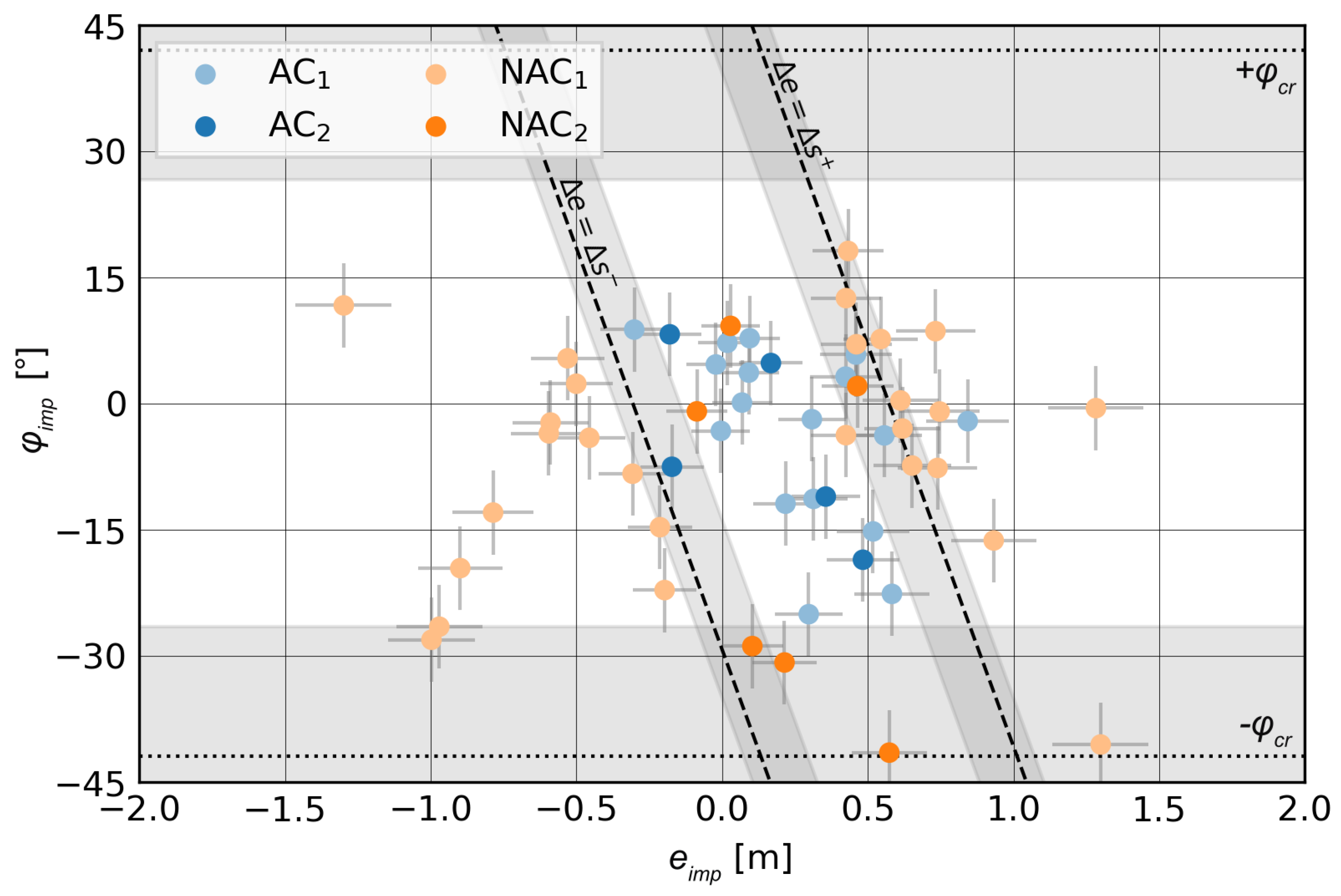
The criterion states that the log accumulation at a circular pier depends on the log’s orientation at the impact (eccentricity $e_{imp}$ and yaw ${\phi }_{imp}$) and its dimension (log length $L_L$) as well as the pier characteristics (diameter $d_p$ and friction coefficient $\mu$) and the hydraulics around the pier (flow velocities $u_1$ and $u_2$). This confirms the governing parameters defined during physical model tests by Schalko et al. [20]. The accumulation criterion is plotted in Figure 15 and compared to the measured values of $e_{imp}$ and ${\phi }_{imp}$. The plot shows that 95% ($n=21$ of 22) of the observed accumulated logs (AC₁ and AC₂) are within the range of $\Delta s^{-}\le \Delta e\le \Delta s^{+}$, while 89% ($n=24$ of 27) of the NAC₁ logs lie outside the range (given $\mu =0.9$). Thus, the accumulation criterion predicts the accumulation behavior of AC₁, AC₂, and NAC₁ logs very well. In contrast, the accumulation behavior of all $n=6$ NAC₂ was predicted incorrectly as these logs were not observed to accumulate (given $\mu =0.9$). While the fact that they lie within the range of $\Delta s^{-}\le \Delta e\le \Delta s^{+}$ explains why they exhibited a very similar behavior as AC₁ logs (slow and bidirectional rotation) and comparably long accumulation times $t_{acc}=\left[20,70\right]$ $\mathrm{s}$ (Table 2), their separation from the pier cannot be explained by the criterion.

The comparison of the accumulation criterion with the field test data shows that the criterion can explain the behaviour of 82% of the cases ($n=45$ out of 55). Furthermore, the criterion is consistent with laboratory investigations that showed that increasing pier diameter $d_p$ and friction coefficient $\mu$ lead to higher accumulation probability [18,20].

In contrast to previous laboratory experiments under uniform flow velocities $u=u_1=u_2$, the novel criterion also takes into account nonuniform flow velocities $u_1\ne u_2$. The criterion shows that under nonuniform conditions only the equilibrium eccentricity $e_{equ}$ changes. The accumulation criterion is astatic approach and some effects that were observed in the laboratory cannot be explained by the criterion. For example, in the laboratory experiments it was found that the log length and the flow velocity have a governing effect on the accumulation probability [20], but this is not fully reflected by the accumulation criterion. While the log length and the flow velocities are parameters of the criterion, higher flow velocities do not affect the accumulation process according to the criterion. Furthermore, it can be hypothesized that additional factors such as the log shape (e.g., bent logs), irregularities on the log surface (roughness, bark, and knotholes), as well as turbulent flow features play a role in the accumulation process that cannot be captured by this static approach.

We assume that the influence of the log length and the flow velocity may be explained by a dynamic model approach. By analyzing the sum of moments $M_{tot}=M_1+M_2$ and the log’s moment of inertia $I_A$ at the contact point, it can be deduced that the angular acceleration $d\phi /d{t}^2=M_{tot}/I_A$ is proportional to the velocity $u^2$ and inversely proportional to $L_L^2$. However, this has not been investigated in depth because the field data are not sufficient to account for different log lengths and flow velocities. The dynamic relationship between log length, flow velocity, and accumulation probability would require further investigation.

4. Conclusions and Outlook

A field test at the River Glatt (Zurich, Switzerland) was conducted to improve the process understanding of LW accumulations at a bridge pier and to evaluate the upscaling of existing flume experiments [20]. The field test demonstrated that the LW accumulation process can be described by three phases: the impact phase, rotation phase, and the separation phase. By combining a simplified equilibria of acting forces and moments, we derived an analytic criterion to describe why a log may accumulate at a bridge pier or not. The existing simplified force system by Schalko [18] was extended to account for nonuniform flow conditions. Based on the force system, a log remains accumulated if the parallel component of the total hydraulic drag force is greater than the friction force between the log and the pier. The resulting critical yaw ${\phi }_{cr}$ of the log for which the friction force is just large enough to compensate the hydraulic drag force is a function of the static friction coefficient $\mu$. The maximum distance $\Delta s$ a log can rotate along the pier before separation is increasing with pier diameter $d_p$ and friction coefficient $\mu$, thereby increasing the accumulation probability p and confirming previous laboratory investigations [20]. Based on the equilibria of moments, the eccentricity for which a log is in equilibrium $e_{imp}$ and does not rotate around the pier is governed by the log length $L_L$ and flow velocities u. We applied the analytic criterion to the field data and demonstrated that it can explain the behavior of 82% of the logs. In addition, the design equation to estimate the accumulation probability p at a single bridge pier by Schalko et al. [20] was applied to the field conditions and validated by the observed accumulation probability (i.e., p = 44% compared to 40%), thereby confirming the applicability of the design equation by Schalko et al. [20] under prototype conditions. In addition, potential scale effects due to the lower drag coefficients for prototype conditions did not affect the resulting accumulation probability p. The similar observations and results between the field and laboratory further highlight the applicability of laboratory studies to investigate LW processes and in particular LW–structure interactions.

The presented accumulation criterion is characterized by a static approach. We hypothesize that the effect of the log length $L_L$ and flow velocity u may only be fully explained by a dynamic model approach. To further improve the process understanding of LW–structure interactions, additional field tests are required with an extended parameter range consisting of various LW characteristics (i.e., log length, log diameter, irregular logs, and varying decomposition) and flow conditions as well as more detailed analyses of the log movement at the pier.

References

- Lucía, A.; Comiti, F.; Borga, M.; Cavalli, M.; Marchi, L. Dynamics of large wood during a flash flood in two mountain catchments. Nat. Hazards Earth Syst. Sci. Discuss. 2015, 3, 1643–1680. [Google Scholar] [CrossRef]
- Keller, E.A.; Swanson, F.J. Effects of large organic material on channel form and fluvial processes. Earth Surf. Process. 1979, 4, 361–380. [Google Scholar] [CrossRef]
- Bezzola, G.; Hegg, C. Ereignisanalyse Hochwasser 2005, Teil 1—Prozesse, Schäden und erste Einordnung (“Analysis of 2005 Flood, Part 1—Processes, Damages, and Classification”); Technical Report 0707; Federal Office for the Environment (FOEN), Eidgenössische Forschungsanstalt WSL: Bern, Switzerland; Birmensdorf, Switzerland, 2007. [Google Scholar]
- Ravazzolo, D.; Mao, L.; Mazzorana, B.; Ruiz-Villanueva, V. Brief communication: The curious case of the large wood-laden flow event in the Pocuro stream (Chile). Nat. Hazards Earth Syst. Sci. 2017, 17, 2053–2058. [Google Scholar] [CrossRef] [Green Version]
- Diehl, T.H. Potential Drift Accumulation at Bridges; US Department of Transportation, Federal Highway Administration, Research and Development, Turner-Fairbank Highway Research Center: McLean, VA, USA, 1997.
- Lyn, D.; Cooper, T.; Yi, Y.; Sinha, R.; Rao, A. Debris Accumulation at Bridge Crossings: Laboratory and Field Studies; Joint Transportation Research Program; Indiana Department of Transportation and Purdue University: West Lafayette, Indiana, 2003; p. 48. [Google Scholar]
- Bocchiola, D.; Rulli, M.; Rosso, R. Transport of large woody debris in the presence of obstacles. Geomorphology 2006, 76, 166–178. [Google Scholar] [CrossRef]
- Schmocker, L.; Hager, W.H. Probability of Drift Blockage at Bridge Decks. J. Hydraul. Eng. 2011, 137, 470–479. [Google Scholar] [CrossRef]
- Gschnitzer, T.; Gems, B.; Mazzorana, B.; Aufleger, M. Towards a robust assessment of bridge clogging processes in flood risk management. Geomorphology 2017, 279, 128–140. [Google Scholar] [CrossRef]
- De Cicco, P.N.; Paris, E.; Ruiz-Villanueva, V.; Solari, L.; Stoffel, M. In-channel wood-related hazards at bridges: A review: In-channel wood-related hazards at bridges: A review. River Res. Appl. 2018, 34, 617–628. [Google Scholar] [CrossRef]
- De Cicco, P.N.; Paris, E.; Solari, L.; Ruiz-Villanueva, V. Bridge pier shape influence on wood accumulation: Outcomes from flume experiments and numerical modelling. J. Flood Risk Manag. 2020, 13. [Google Scholar] [CrossRef]
- Panici, D.; de Almeida, G.A.M. Formation, Growth, and Failure of Debris Jams at Bridge Piers. Water Resour. Res. 2018, 54, 6226–6241. [Google Scholar] [CrossRef]
- Panici, D.; de Almeida, G.A.M. Influence of Pier Geometry and Debris Characteristics on Wood Debris Accumulations at Bridge Piers. J. Hydraul. Eng. 2020, 146, 04020041. [Google Scholar] [CrossRef]
- Panici, D.; Kripakaran, P.; Djordjević, S.; Dentith, K. A practical method to assess risks from large wood debris accumulations at bridge piers. Sci. Total Environ. 2020, 728, 138575. [Google Scholar] [CrossRef] [PubMed]
- Panici, D.; de Almeida, G.A.M. A theoretical analysis of the fluid–solid interactions governing the removal of woody debris jams from cylindrical bridge piers. J. Fluid Mech. 2020, 886, A19. [Google Scholar] [CrossRef]
- Schalko, I. Large Wood Accumulation Probability at a Single Bridge Pier. In Proceedings of the 37th IAHR World Congress, Kuala Lumpur, Malaysia, 13–18 August 2017. [Google Scholar] [CrossRef]
- Schalko, I.; Schmocker, L.; Weitbrecht, V.; Boes, R.M. Risk reduction measures of large wood accumulations at bridges. Environ. Fluid Mech. 2020, 20, 485–502. [Google Scholar] [CrossRef]
- Schalko, I. Modeling Hazards Related to Large Wood in Rivers. Ph.D. Thesis, Versuchsanstalt für Wasserbau, Hydrologie und Glaziologie (VAW), ETH Zurich, Zurich, Switzerland, 2018. [Google Scholar] [CrossRef]
- Braudrick, C.A.; Grant, G.E.; Ishikawa, Y.; Ikeda, H. Dynamics of wood transport in streams: A flume experiment. Earth Surf. Process. Landforms 1997, 22, 669–683. [Google Scholar] [CrossRef]
- Schalko, I.; Schmocker, L.; Weitbrecht, V.; Boes, R.M. Laboratory study on wood accumulation probability at bridge piers. J. Hydraul. Res. 2020, 58, 566–581. [Google Scholar] [CrossRef]
- AWEL. Discharge data sheet of the River Glatt at Dübendorf, Switzerland. 2020. Available online: https://tinyurl.com/ym9f5r7w (accessed on 20 August 2021).
- Swain, M.J.; Ballard, D.H. Indexing via color histograms. In Active Perception and Robot Vision; Springer: Berlin/Heidelberg, Germany, 1992; pp. 261–273. [Google Scholar]
- Thielicke, W.; Stamhuis, E.J. PIVlab—Towards User-friendly, Affordable and Accurate Digital Particle Image Velocimetry in MATLAB. J. Open Res. Softw. 2014, 2, 30. [Google Scholar] [CrossRef] [Green Version]
- Achenbach, E.; Heinecke, E. On vortex shedding from smooth and rough cylinders in the range of Reynolds numbers 6× 10³ to 5× 10⁶. J. Fluid Mech. 1981, 109, 239–251. [Google Scholar] [CrossRef]
- Möhler, K.; Herröder, W. Obere und untere Reibbeiwerte von sägerauhem Fichtenholz (“Upper and lower friction coefficients of spruce wood”). Holz als Roh-und Werkstoff 1979, 37, 27–32. [Google Scholar] [CrossRef]
- Jaaranen, J.; Fink, G. Frictional behaviour of timber-concrete contact pairs. Constr. Build. Mater. 2020, 243, 118273. [Google Scholar] [CrossRef]
Figure 1.
Naturally formed LW accumulation at the test site (River Glatt) in February, 2021. Flow direction from bottom to top.
Figure 2.
(a) Test site at the River Glatt with a log being placed upstream of the bridge pier by a truck crane with discharge Q, log length , and pier diameter , and (b) log storage prior to the log placement in the river.
Figure 3.
(a) Streamwise surface velocity u at the test site. Note that u is generally higher towards the right bank than towards the left bank due to the slight left bend of the River Glatt. Vertical lines illustrate location of lateral profiles. (b) Lateral profiles of u at distances of , and from the upper edge of the pier.
Figure 4.
Manual detection of log orientation with (a) snapshot of log at impact point with reference points P1 to P4, (b) perspective transformation of the snapshot, and (c) cropped section of the perspective transformation with manually detected log endpoints (P5 and P6).
Figure 5.
Automatic detection of log orientation with (a) cropped section of a perspectively transformed snapshot, (b) log detection using histogram backprojection, and (c) image dilation and fitting of a straight line to determine the yaw . Note that the color of the log should be easily distinguishable from the color of the water that surrounds the log. Therefore, the automatic detection was conducted for selected logs only.
Figure 6.
Schematic overview of the accumulation process of a single log at a bridge pier with the three phases impact, rotation, separation, and their subprocesses. The values in brackets indicate an approximate time-scale for the process duration based on video observations.
Figure 7.
Histograms of (a) log impact eccentricity and (b) impact yaw .
Figure 8.
Accumulation time versus (a) impact eccentricity and (b) impact yaw for accumulated and not accumulated logs.
Figure 9.
Snapshot series of an initial log submergence. After the log impact on the pier (), a water wave was generated and spilled over the log () while the log changes its vertical position to a partially submerged position ( and later).
Figure 10.
Histograms of (a) impact eccentricity , (b) impact yaw , and (c) final yaws at separation point (NAC logs) or in equilibrium (AC logs); the dotted lines indicate the critical yaw .
Figure 11.
Log rotation of selected AC1 logs during their rotation phase at the pier.
Figure 12.
Streamwise surface velocity u in the vicinity of the pier for (a) log #7 with , (c) log #22 with accumulated at the pier, and snapshots of (b) log #7 and (d) log #22 during PIV measurement.
Figure 13.
Definition sketch of the acting forces on a log with eccentricity e and yaw .
Figure 14.
(a) Sketch of the critical yaw for . Logs can only accumulate if they impact with a yaw between (blue area) and do not rotate further than or , respectively. (b) Illustration of the rotation of a log from its eccentricity at the impact point to the equilibrium eccentricity with .
Figure 15.
Comparison of the measured log orientation ( and ) with the accumulation criterion . A total of 95% of the observed accumulated logs (AC1 and AC2) lie within the predicted range, while 89% of the NAC1 logs lie outside the range. The NAC2 logs are poorly predicted by the criterion. The criterion was evaluated with and the gray areas reflect the uncertainty in ranging from 0.5 to 1.1 [26]. Error bars of (position accuracy of P3) for and for are plotted in gray.