
Chlorophyll and Suspended Solids Estimation in Portuguese Reservoirs (Aguieira and Alqueva) from Sentinel-2 Imagery


1
Department of Biology, Faculty of Sciences, University of Porto (FCUP), Rua do Campo Alegre s/n, 4169-007 Porto, Portugal
2
Centre of Molecular and Environmental Biology (CBMA), Department of Biology, University of Minho, Campus of Gualtar, 4710-057 Braga, Portugal
3
Institute of Science and Innovation for Bio-Sustainability (IB-S), Campus of Gualtar, University of Minho, 4710-057 Braga, Portugal
4
Image Processing Laboratory, Universitat de València, C/Catedrático José Beltrán Martínez, 2, 46980 València, Spain
5
CIIMAR—Interdisciplinary Centre of Marine and Environmental Research, Terminal de Cruzeiros do Porto de Leixões, Avenida General Norton de Matos s/n, 4450-208 Matosinhos, Portugal
*
Author to whom correspondence should be addressed.
Water 2021, 13(18), 2479; https://doi.org/10.3390/w13182479
Submission received: 2 August 2021
/
Revised: 3 September 2021
/
Accepted: 6 September 2021
/
Published: 9 September 2021
(This article belongs to the Special Issue Methods for Assessing Water Quality and Its Impacts on Ecological Status in Reservoirs)
Abstract
:Reservoirs have been subject to anthropogenic stressors, becoming increasingly degraded. The evaluation of ecological potential in reservoirs is remarkably challenging, and consistent and regular monitoring using the traditional in situ methods defined in the WFD is often time- and money-consuming. Alternatively, remote sensing offers a low-cost, high frequency, and practical complement to these methods. This paper proposes a novel approach, using a C2RCC processor to analyze Sentinel-2 imagery data to retrieve information on water quality in two reservoirs of Portugal, Aguieira and Alqueva. We evaluate the temporal and spatial evolution of Chl a and total suspended solids (TSS), between 2018 and 2020, comparing in situ and satellite data. Generally, Alqueva reservoir allowed lower relative (NRMSE = 8.9% for Chl a and NRMSE = 21.9% for TSS) and systematic (NMBE = 1.7% for Chl a and NMBE = 2.0% for TSS) errors than Aguieira, where some fine-tuning would be required. Our paper shows how satellite data can be fundamental for water-quality assessment to support the effective and sustainable management of inland waters. In addition, it proposes solutions for future research in order to improve upon the methods used and solve the challenges faced in this study.
1. Introduction
Despite only covering a relatively small area of the planet’s surface—estimated to cover ~3% of the terrestrial surface of Earth—inland waters have great importance for numerous critical functions, since they provide ecosystem services such as hydroelectricity production, flood control, navigation, water supply, and fisheries [1,2,3]. These water bodies provide services that influence human welfare, directly and indirectly, and, therefore, they emerge as a limiting factor in quantity and quality for human development and ecological stability [4,5]. In addition, inland water bodies act as sentinels of the ever-changing environment in their surroundings, reporting the status of phenomena such as climate change, developmental pressure, and land-use and land-cover change [6]. Reservoirs are a distinct example of inland water bodies and are an easy target for waste disposal. Currently, freshwater ecosystems show an increase in degradation in water quality and ecosystem services due to human activities. Soil occupation, agriculture, urbanization, and industrial affairs comprise actions already described to affect these water bodies [6]. So, reservoirs are subject to a wide diversity of anthropogenic stressors, making it necessary to evaluate reservoir ecosystem changes and to understand the magnitude and implications of these alterations [7].
In order to protect and manage aquatic ecosystems, the Water Framework Directive 2000/60/EC (WFD), European legislation in the water policy and quality, requires each European Union (EU) member state to assess the quality of their water bodies (e.g., rivers and reservoirs) [8]. The WFD classifies reservoirs as heavily modified water bodies (HMWB) due to physical alterations caused by human activity, substantially changing them in character [8]. Traditionally, the ecological status of water bodies is defined according to their biological, chemical, and physical characteristics in comparison with reference values [9]. However, for natural water bodies, the reference condition is their high ecological status (HES), while for HMWB it is the maximum ecological potential (MEP) [10]. According to the WFD, the MEP is defined as the state where “the values of the relevant biological quality elements reflect, as far as possible, those associated with the closest comparable surface water body type, given the physical conditions, which result from the heavily modified characteristics of the body” [10].
The evaluation of ecological potential in reservoirs is remarkably challenging due to their complex nature, which represents an environment different from lakes and rivers [9,11,12]. Besides, consistent monitoring using the metrics defined in the WFD follows traditional in situ methods (e.g., water sample collection and laboratory analysis) that are often very time and money consuming to estimate the quality of water regularly [13]. The WFD implementation has required a large expansion in the monitoring of water bodies which made it possible to perceive their ecological status. Indeed, many researchers advocate some change in the WFD-monitoring measures to provide sufficient spatial and temporal resolution, and, in many cases, to make it more cost-effective [14]. In recent years new monitoring tools have become available, including Earth Observation [15,16]. The use of satellite data for monitoring has demonstrated a high potential to better standardize measures across Europe. This approach has been recognized by several authors through enhancing both spatial coverage and frequency of monitoring of variables, such as water color, chlorophyll a (Chl a), cyanobacteria, and emergent macrophyte coverage [16].
Since the 1960s, remote sensing (RS) techniques have been used to monitor aquatic environments, by analyzing ocean color under the assumption that Chl a—a proxy for phytoplankton biomass quantification—and surface temperature could be estimated remotely [17,18]. Based on this, oceanographers started to remotely monitor the optical properties of waters’ constituents, such as phytoplankton, colored dissolved organic matter (CDOM), and total suspended solids (TSS) [19,20]. However, the application of RS techniques to inland waters remains a challenge. In general, less success is recognized when applying RS techniques for monitoring inland water bodies’ quality, due to their distinct shapes and sizes, the comparably more significant impact of their border effect, and the variable composition of water constituents [6]. Alternatively, satellite RS techniques have been used as an effective tool for supporting the implementation of the WFD [21]. Today, there are a plethora of programs that make use of satellite RS technologies, such as the Copernicus Program. This is an EU-led initiative designed to establish a European capacity for the provision and use of operational monitoring information for environmental and security applications [22]. Within the Copernicus Program, the European Space Agency (ESA) is responsible for the development of the Space Component. The Sentinel missions are Copernicus dedicated Earth Observation missions, composing the essential elements of the Space Component [22,23,24,25]. The Sentinel-2 mission provides continuity to services relying on multispectral high-spatial-resolution optical observations over global terrestrial surfaces [22]. Sentinel-2 A and Sentinel-2 B are the two polar-orbiting satellites that comprise the Copernicus Sentinel-2 mission. This mission aims at monitoring variability in land surface conditions and makes use of its wide swath width (290 km) and high revisit time (5 days with the two satellites under cloud-free conditions at the equator, which results in 2–3 days at mid-latitudes) to support monitoring of Earth’s surface changes [26]. Each satellite is equipped with a multispectral instrument (MSI) that works passively by collecting sunlight reflected from the Earth. This instrument is responsible for measuring Earth’s reflected radiance in 13 spectral bands, with 10 and 20 m spatial resolution and 3 bands at 60 m for atmospheric correction [26].
Despite the capabilities of today’s satellite RS technologies, their direct products do not represent a sufficiently reliable portrait of the Earth’s surface. Satellites measure the light field emerging at the top-of-atmosphere, and thus an atmospheric correction (AC) needs to be performed as part of the processing of water-body data [27]. Due to the low reflectivity of water, around 90% of the signal that reaches satellite sensors is affected by the absorption and scattering by different particles present in the atmosphere (e.g., water vapor, ozone, oxygen, carbon dioxide and aerosols) [13]. The atmospheric path traveled by the generally low radiances at the water’s surface makes the requirements for AC very demanding [27]. However, AC processors can remove the scattered signal of the atmosphere and retrieve the signal from the water’s surface [28,29]. The Case 2 Regional Coast Color (C2RCC) is an AC processor made available through ESA’s Sentinel Toolbox Sentinel Application Platform (SNAP). It relies on a database of radiative transfer simulations, inverted by neural networks. The core is a five-component inherent-optical-properties (IOP) model that was derived from the NASA bio-Optical Marine Algorithm Data set in situ measurements. C2RCC has been validated for the different sensors, with good results for Case 2 waters, as well as possessing special neural nets, such as C2X-Nets, which is trained for extremeIOP ranges [27].
Ongoing developments in RS and geographical information science massively improve the efficiency in analyzing Earth’s surface features. The increased frequency of image acquisition together with the advances in the ability to process data provides new opportunities to understand the complex inland water systems [30]. Modabberi et al. (2020) provided the first evaluation of the spatiotemporal variation of Chl a across the Caspian Sea, as this water body had been subject to increasing pollution and environmental degradation [31]. The authors made use of Level 3 MODIS-Aqua Chl a data from January 2003 to December 2017 to discover that this water body had suffered from a growing increase in Chl a, especially in warmer months [31]. Modabberi et al. (2020) concluded that these trends reflect the increasing rate of degradation in the Caspian Sea [31]. Ansper and Alikas (2019) used 89 Estonian lakes in a study that aimed to analyze the suitability of Sentinel-2 MSI data to monitor water quality in inland waters [13]. The authors concluded that, despite their methods being able to provide complementary information to in-situ data to support WFD monitoring requirements, it is important to note that ACs are sensitive to surrounding land and often fail in narrow and small lakes [13]. In the Iberian Peninsula, Sòria-Perpinyà et al. (2019) worked on Albufera de València—a hypertrophic lake in Valencia, Spain—that aimed to demonstrate the validity of an algorithm for Chl a concentration retrieval from Sentinel-2 MSI [32]. With the results obtained, the authors were able to infer that the temporal evolution of Chl a concentration variations followed an annual bimodal pattern [32]. In Portugal, Potes et al. (2018) used the Alqueva reservoir as a study site to assess the use of the Sentinel-2 MSI for water quality monitoring [33]. Despite the set of algorithms being applied with good results, some tuning of the algorithms used was still required to make use of the full potential of the MSI [33].
Despite challenging, the use of RS technologies may be an essential alternative, opposed to using exclusively traditional field-based methods to monitor water quality, as they offer a comparatively low-cost, high frequency, spatially extensive and practical complement for water-quality assessment and monitoring [34,35].
In this work we will focus on the study of the temporal and spatial evolution of Chl a and TSS, between the years 2018 and 2020, in order to show the validity of a proposed tool for Sentinel-2 images and an operative method for the multitemporal study in different reservoirs of Portugal: Aguieira and Alqueva. Specifically, we applied the C2RCC AC processor to Sentinel-2 imagery data aiming to (i) assess the portability of this AC processor between different reservoirs, and (ii) validate its use for a rapid assessment of water quality.
2. Materials and Methods
2.1. Study Area
Two Portuguese reservoirs were selected to conduct this study—Aguieira and Alqueva (Figure 1)—as they are included in a national project, ReDEFine (POCI-01-0145-FEDER-029368), which focuses on multiscale and multistep tools for the assessment of reservoir-water quality, to fill existing gaps in the current approach by the WFD.
The Aguieira reservoir is in Coimbra district (central Portugal) (Figure 1A) and is integrated into the municipalities of Carregal do Sal, Mortágua, Penacova, Santa Comba Dão, Tábua, and Tondela. This water body—the biggest reservoir in central Portugal (area ≈ 20 km2)—is inserted in the Mondego hydrographic basin, at the confluence of two secondary rivers, Dão and Criz. The Aguieira reservoir has a drained area ≈ 300,000 ha, and its dam started operating in 1981 with the purposes of energy production, irrigation, and water storage [36,37,38,39]. In the sampling period, water level recorded in this reservoir varied between 113.99 m (on the 25 January 2020) and 177.51 m (on the 14 December 2018). In its vicinity, there are food, textile, wood, and cork industries. The surrounding landscape is dominated by eucalyptus, acacias, pines, agricultural soils, moors, and bushes [38,40,41]. The climate of this region is strongly influenced by Mediterranean conditions, being characterized by mild/cold winters and hot summers [36,38,42]. This reservoir presents characteristics of a hot monomictic lake, mixing only once (in the cold periods), as well as sometimes periods of strong thermal stratification regarded in the coldest and hottest periods [36]. Moreover, this reservoir is included in the inter-calibration study for the WFD.
The Alqueva reservoir—the biggest artificial lake in southern Europe (area ≈ 250 km2)—is in the Beja and Évora districts (southern Portugal) (Figure 1Al) and is within the municipalities of Portel and Moura. It is integrated within the Multipurpose Alqueva Project (MAP), which includes almost 70 reservoirs in this water-scarce region of the country [43]. This reservoir is inserted in the Guadiana hydrographic basin, following the waterline of the Guadiana River. The Alqueva reservoir has a drained area of ≈5500.000 ha, and the dam started to fill up in 2002 [44]. In the sampling period, water level recorded in this reservoir varied between 145.02 m (on the 13 December 2019) and 148.72 m (on the 9 December 2018). The reservoir is used for energy production, irrigation, and water-storage purposes. In its vicinity, there are some commercial or industrial units. The surrounding landscape is composed of non-irrigated arable lands, permanently irrigated land, fruit trees and berry plantations, olive groves, complex cultivation patterns, agro-forestry areas, broad-leaved forest, and coniferous forest [45]. The climate of this region is classified as a Csa Region according to the Köppen climate classification, which corresponds to a Mediterranean climate (i.e., a temperate climate with dry, hot summers) [43,46].
2.2. Materials
2.2.1. In Situ Data
For the in-situ data collection, several sampling points were selected at each reservoir (four sites in Aguieira reservoir and five sites in Alqueva reservoir—Figure 1). These sites are located along the bank of the reservoirs and were selected based on accessibility and previous monitoring stations (defined by the agency for the monitoring program, Sistema Nacional de Informação de Recursos Hídricos (SNIRH)) [44]. The samplings were carried out in four periods across 2018, 2019, and 2020 (Table 1). In Situ, with a multiparameter probe (Multi 3630 IDS SET F), some general physical and chemical parameters were measured sub-superficially (<0.5 m of depth): pH, dissolved oxygen (O2, mg L−1 and %), conductivity (Cond, μS cm−1), and temperature (Temp, °C). Additionally, in each site, water samples were collected and transported to the laboratory under thermal conditions (at 4 °C and in the dark) for further analysis. Water samples were used to determine: the five-days biochemical oxygen demand (BOD5, mg L−1), the volatile suspended solids (VSS- mg L−1), the turbidity (Turb, m), the dissolved organic carbon (DOC, m−1), the title hydrometric (TH, °f), ironiron (Fe, μg L−1), manganese(Mn, μg L−1), arsenic(As, μg L−1), cadmium (Cd, μg L−1), copper (Cu, μg L−1), mercury (Hg, μg L−1), nickel (Ni, μg L−1), lead (Pb, μg L−1), zinc (Zn, μg L−1), chemical oxygen demand (COD, mg L−1), ammonium (NH4, mg L−1), Kjedahl nitrogen nitrogen (N, mg L−1), nitrate (NO3, mg L−1), nitrite (NO2, mg L−1) and phosphorus (P, mg L−1). For determination of the content of TSS and Chl a, water samples were filtered through a Whatman GF/C filter (47 mm diameter and 1.2 μm pore). Three filters, with the seston of each site, were used to determine the TSS according to APHA (1989) [47]. Chl a extraction from the filters was performed according to the Lorenzen (1967) method [48]. In this work, the term “total suspended matter” (TSM) is also used. Indeed, authors may use differing terms, but TSS and TSM are equivalent and interchangeable terms used to describe organic (autotrophic and heterotrophic plankton, bacteria, viruses, and detritus) and mineral particles [49]. The term “TSM” is used in this work when referred to content of different authors, in order to be coherent with their work.
For determination of general physical and chemical parameters, iron and manganese, trace elements and mineral elements, oxygen and organic compounds and nitrogenous and phosphorous parameters, samples from Aguieira and Alqueva were processed by Eurofins Lab Environment Testing Portugal, Unipessoal LDA. Hence, the quality of the analyses is assured by the company.
2.2.2. Sentinel-2 Multispectral Imagery Data Collection
The present work used Sentinel-2 satellite data from the two polar-orbiting satellites that comprise the Copernicus Sentinel-2 mission. Images were downloaded using the Copernicus Open Access Hub [50], from 2018 to 2020. Some satellite imagery was discarded to avoid misinterpretation, due to the presence of haze or cirrus clouds above the reservoirs. This resulted in the unavailability of imagery data concerning autumn of 2019 in the Aguieira reservoir. No data concerning this instance is represented in the results nor is it used in statistical analysis. Ideally, in-situ samplings should be conducted on the same day as images will be available, or with very few days apart. Notwithstanding, the high temporal resolution (10 days using one satellite, 5 days using two) offered by Sentinel-2 satellites allowed to achieve seven valid observations i.e., completely cloud-free scenes that represented the entire reservoirs. The match-ups made with the in-situ sampling dates are presented in Table 1.
2.3. Methodology
2.3.1. Processing and Outputs: C2RCC in SNAP
Chl a and TSS concentrations were obtained via satellite imagery based on the proposed steps, following the RS approach reported in Figure 2. Firstly, the downloaded images were loaded into SNAP, and subsets that contained the reservoirs were created to reduce file size. Secondly, each image was resampled to different spatial resolutions at 20 m and 60 m, since this will allow assessing the impact of the border effect at different spatial resolutions. Thirdly, each resample was processed with C2RCC, applying ACs according to the default parameters except for the neural nets, which were changed to “C2X-Nets”. The C2RCC processor was used through SNAP v8.0 [51]. The change of neural nets is due to some sites being very eutrophicated and, as previously mentioned, this neural net is trained for extreme IOP ranges. Afterward, a land/sea mask was applied to each corrected resample using a shapefile of the reservoirs, reducing the file to the area of interest (AOI). Finally, pixel values were extracted using pins with the coordinates of the sampling sites.
Among the many products generated by SNAP when performing the C2RCC AC, we focus on two products: the bands “conc_chl” and “conc_tsm”. From these bands it is possible to extract the product values for Chl a (mg m−3) and TSS (g m−3), respectively, which will be used in the statistical analysis.
2.3.2. Data Analysis
Firstly, in order to assess differences between reservoirs, a principal component analysis (PCA) was conducted based on in-situ data collected along the study. To avoid autocorrelation among data, we selected in-situ data based on KMO (Kaiser-Meyer-Olkin) and communalities. The KMO measures the proportion of variance among the variables that can be derived from the common variance, also called systematic variance [52]. KMO is computed between 0 and 1 [52]. Low values (close to 0) indicate that there are large partial correlations in comparison to the sum of the correlations, that is, there is a predominance of correlations of the variables that are problematic for the principal component analysis [52]. Hair et al. (2018) suggest that individual KMOs smaller than 0.5 be removed from the principal component analysis. Consequently, this removal causes the overall KMO of the remaining variables of the factor/principal component analysis to be greater than 0.5 [52].
In addition, we explore the presence of a correlation between Chl a and TSS, in both reservoirs, to assess the range of variation of these variables, based on in-situ data, through scatter plots.
Successively, to evaluate the discrepancies between matching in-situ data and all resolutions of Sentinel-2 products (20 m and 60 m) the normalized root mean squared error (NRMSE) and the normalized mean bias error (NMBE) were calculated according to Equations (1) and (2). The NRMSE is a normalized measure of the relative error (scatter) and the NMBE is the normalized average forecast error representing the systematic error of a forecast model to under or over forecast [53]. NRMSE and NMBE results that revealed low systematic and relative errors would support the validity of the application of C2RCC in the study area. Statistical analysis of the in situ and satellite data, as well as the “match-ups” between both, was performed in R software v3.6.1 [54].
where, Sat and Situ stand for the satellite and in situ data, respectively, and the terms Situmax and Situmin are the maximum and minimum values of in-situ data.
In addition, in order to assess the statistical differences between all sites of each reservoir, concerning the parameters Chl a and TSS, a Kruskal-Wallis test was performed.
3. Results
3.1. In Situ Data & SNAP-C2RCC Estimates
Results obtained for in situ and satellite values in site A3 in Aguieira were very distinct from the remaining sites, considering that in autumn of 2018 the in situ value of Chl a even surpassed 1000 μg L−1. For this reason, site A3 in Aguieira will not be considered for calculating the following statistics nor will their in situ and satellite results be presented.
Before performing the PCA, it is necessary to remove any variables that account for a small proportion of variation in the dataset. According to Hair et al. (2018) we removed individual KMOs smaller than 0.5 and only used communalities greater than 0.5 [52] (see Appendix A, Table A1). Results from Kaiser-Meyer-Olkin (KMO) and communalities tests suggested removing the variables NO3, Temp, pH, COD, Cu, NO2, Zn, Hg, Ni, Cd, and Pb.
The PCA was then computed using in-situ data (see Appendix B, Table A2), with the exclusion of the mentioned variables. In this PCA (Figure 3), Principal Component (PC) 1 explains 44% (eigenvalue = 6.62) of the variation in the dataset and PC 2 explains 20% of the variation (eigenvalue = 3), together explaining over 60% of the variation in the dataset.
In general, PC1 seems to reflect water-quality parameters, whereas PC2 seems to reflect differences between reservoirs based on physical and chemical parameters such as metals. Along PC1, Al5 is the sampling point with higher values of Mn (loading score = 0.332), TSS (loading score = 0.321), N (loading score = 0.32), BOD5 (loading score = 0.316), and VSS (loading score = 0.312). Along PC2, differences between Alqueva and Aguieira seem to increase during the spring (2019 and 2020), particularly influenced by differences in TH (loading score = 0.452), Cond (loading score = 0.438), and AS (loading score = 0.324). While the PCA reveals spatial and temporal variety within Alqueva, it shows that Aguieira is generally more homogenous.
With the purpose of verifying a relation between in situ Chl a and TSS in both reservoirs, and assess the range of variation of these variables, the plots that confront Chl a and TSS in-situ data for both reservoirs are presented in Figure 4.
In both reservoirs the plots suggest a linear relation between Chl a and TSS measured in situ. Nonetheless, the slope in Alqueva′s plot is higher, meaning that, for the same amount of TSS in both reservoirs, there is more Chl a in Alqueva than in Aguieira (Figure 4). These results corroborate the PCA results, in which it was seen that Alqueva observations, particularly site Al5, would have distinct values for variables such as Chl a.
3.2. In Situ Data vs. SNAP-C2RCC Estimates
The results obtained in situ (for additional data see Appendix B, Table A2) and the processing of images using the C2RCC AC processor in SNAP are presented in Table 2. In situ results for Chl a in Aguieira were generally lower in autumn (approximately ranging from 3 to 10 μg L−1) than in spring seasons (approximately ranging from 10 to 42 μg L−1). In Alqueva, in situ results for Chl a recorded less seasonal variation, with similar values for autumn (approximately ranging from 0 to 4 μg L−1) and spring seasons (approximately ranging from 0 to 8 μg L−1). However, a few exceptions were recorded, namely in Al5 (Alqueva) where values were higher than the remaining sites, throughout the autumn and spring seasons.
The in situ results recorded for TSS, in Aguieira, were higher in spring seasons (approximately ranging from 11 to 19 mg L−1) than in autumn (approximately ranging from 8 to 11 mg L−1). In Alqueva, although seasonal variation was similar to Aguieira, the recorded values were, generally, low for both seasons (approximately ranging from 3 to 5 mg L−1 in autumn, and from 6 to 13 mg L−1 in spring). For TSS in Alqueva, Al5 was an exceptional site, for which recorded values were much higher than in any other site, in both autumn and spring seasons.
The range of SNAP-C2RCC results was broad in terms of values across the different resolutions for Chl a and TSS. Across resolutions, satellite results for Chl a in Aguieira were similar between autumn of 2018 and spring of 2019 (approximately ranging from 3 to 42 μg L−1 and 4 to 32 μg L−1, respectively). However, spring of 2020 revealed distinct results with values lower than other seasons (ranging approximately from 0 to 10 μg L−1). Similar to Aguieira, in autumn of 2018 and spring of 2019 the derived Chl a shared an identical range of results (approximately ranging from 8 to 21 mg L−1 and 9 to 24 mg L−1, respectively), while in spring of 2020 it had lower results (approximately ranging from 0 to 5 mg L−1).
Satellite results for Alqueva, for Chl a and TSS, did not reveal seasonal differences in terms of range of values. Nonetheless, it is visible that site Al5 consistently presented much higher values, across both resolutions and all seasons, than any other site. Consistently with in-situ data presented in the PCA (Figure 3), SNAP-C2RCC results also reveal higher values in sampling site Al5.
The Kruskal–Wallis tests results revealed no significant differences between sampling sites within each reservoir, concerning the Chl a and TSS in-situ data recorded, with the exception on Chl a in Alqueva (χ2 [4] =10.44; p-value = 0.034).
The plots that confront in situ results and SNAP-C2RCC results, obtained from Sentinel-2 images, are presented in Figure 5.
The plots in Figure 5 inform that results are heterogenous, i.e., results for a certain instance (e.g., reservoir, site, season, resolution, or variable) may be closer to the ideal scenario than other instances.
The results of the NRMSE and NMBE metrics are presented in Table 3. Regarding the Aguieira reservoir, the values derived with SNAP-C2RCC revealed, in general, high relative and systematic errors. Concerning the TSS parameter, using the 20 m product allowed lower relative errors (NRMSE = 80.3%) as well as lower systematic errors (NMBE = −15.8%) than using the 60 m product (NRMSE = 112% and NMBE = −85.3%). Despite still high, results obtained concerning in situ Chl a and respective satellite variable were generally lower than those for TSS. In terms of relative error, the results were similar between both resolutions (using 20 m NRMSE = 55% and using 60 m NRMSE = 58%). Moreover, using the 20 m product allowed for much lower systematic error (NMBE = −16.4%) than using the 60 m product (NMBE = −43.6%). Across both sets of variables and resolutions, systematic errors were negative, indicating an underestimation of in-situ values by SNAP-C2RCC.
In general, NRMSE and NMBE results were lower for the Alqueva reservoir than the Aguieira reservoir. In Alqueva, regarding the Chl a parameter, using the 20 m product achieved higher relative and systematic errors (NRMSE = 16.7% and NMBE = −4.2%, respectively) than using the 60 m product. Regarding the TSS parameter, using the 60 m product allowed for lower errors (NRMSE = 21.9% and NMBE = 2.0%) (Figure 6b) than using the 20 m product (NRMSE = 32% and NMBE = 7.2%).
Results were the closest to the ideal scenario for the Alqueva reservoir, where low relative and systematic errors were found. An example of the best results obtained in this study is showed in Figure 6, using the 60 m product to estimate Chl a and TSS in Alqueva. As it can be seen on both plots, most observations are aggregated between the values 0 to 20 μg L−1 for Chl a and 0 to 20 mg L−1 for TSS. The latter allowed the best results obtained across all resolutions, parameters, and reservoirs with a low relative error (NRMSE = 8.9%) and even lower systematic error (NMBE = 1.7%) (Figure 6a).
4. Discussion
Inland water RS has faced, and continues to face, many challenges, not only in terms of the science underpinning the retrieval of physical and biogeochemical properties over typically highly optically complex waters, but it has also suffered from lack of funding, infrastructure, and the mechanisms needed to coordinate research efforts across an historically fragmented community [55]. This has meant that the inland water community has often had to make use of data from satellite sensors designed primarily for land applications. While these sensors have adequate spatial resolutions for some water bodies, their spectral coverage and resolution are not optimal for many applications over inland waters (e.g., CDOM retrieval). The optical complexity of inland waters, AC issues and adjacency effects add additional challenges to inland water RS [55]. In this section, such challenges are approached, in order to assess their influence on the results and further improve the methods.
Regarding the spatial differences between both reservoirs, data from NRMSE and NMBE metrics for Alqueva showed interesting results. For Chl a and TSS, NRMSE results were as high as 32% and as low as 8.9%, indicating a slight relative error (slight scatter of observations). As for the NMBE results, their values were even lower than the NRMSE, ranging from 4.2% to 7.2%. This means that systematic errors were very low and that in most observations there was a slight overestimation of in-situ data by the satellite products, except for Chl a when using the 20 m product which indicated a slight underestimation. The Chl a variable is commonly used as a proxy for the phytoplankton biomass present in a water body [17,18]. Hence, this study showed that, in Alqueva, phytoplankton is a more predominant component of suspended solids and, therefore, contributes more to water turbidity than in Aguieira. In particular, the most interesting results came out of applying C2RCC to Sentinel-2 MSI 60 m products in Alqueva. This is the case for both parameters. Although further research is needed to investigate the reasons behind Aguieira’s higher errors, Alqueva’s results indicate that satellite data can be very useful and reliable for monitoring reservoirs.
Plowey (2019) in a study using Sentinel-3 Ocean and Land Color Instrument (OLCI) imagery of lakes, achieved low errors for Chl a retrieval (NMBE = −7%, RMSE = 40%, n = 156), but high errors when retrieving TSM by using the standard C2RCC neural network [56]. Moreover, Kyryliuk and Kratzer (2019) in a study using Sentinel-3 OLCI imagery of the Baltic Sea, demonstrated that Chl a was retrieved with a relatively low systematic error (NMBE = 10%), but a high relative error (RMSE = 97%, n = 26) [57]. However, similarly to Plowey (2019), the authors observed a large systematic error (NMBE = 103%) and an even larger relative error (RMSE = 167%), when retrieving TSM [56,57]. In contrast to both studies, where problems were reported when retrieving TSM, this factor was not an obstacle in this study. In addition, Kyryliuk and Kratzer (2019) found that their results improved when studying the regional specific IOPs of their study area and using them to better configure C2RCC [57]. This could constitute a solution to obtain more reliable results when monitoring reservoirs, particularly ones of smaller dimensions such as Aguieira. However, it is important to keep in mind that the metrics used are normalized by the range of observed in-situ data to allow for comparable results.
The optical properties of inland waters are highly variable between, and even within, water bodies. These issues confound the development of algorithms for inland waters and typically limit their applicability to different water bodies [55]. Johansen et al. (2018) evaluated the performances of 29 algorithms that use satellite-based spectral imager data to derive estimates of Chl a that, in turn, can be used as an indicator of the general status of algal cell densities and the potential for cyanobacterial harmful algal blooms (CHABs) [58]. They aimed to identify algorithm-imager combinations that had a high correlation with coincident Chl a surface observations for two temperate inland lakes, as it suggested portability for regional CHAB monitoring [58]. Even though the two lakes were different in terms of background water quality, size and shape, and the results obtained support the portability of using a suite of certain algorithms across multiple sensors to detect potential algal blooms using Chl a as a proxy [58].
In the same line of thought, we also aim to assess the portability of the application of the C2RCC processing chain between the studied reservoirs. For this purpose, the spatial differences between the reservoirs should be considered. From the PCA using in-situ data from both reservoirs we concluded that, except for sampling site Al5, both reservoirs were similar in terms of physical and chemical parameters (Figure 3). Hence, their dimensions are the biggest difference between themselves. As a reminder, while Aguieira only occupies a drained area of ≈300,000 ha, Alqueva is over ten times bigger, occupying a drained area of ≈5500.000 ha. In addition, it is also important to consider the geographic location of both reservoirs—Aguieira is located in the center of Portugal and Alqueva is located in southern Portugal. Yet, IOPs vary not only across geographic regions but also within the same water mass [5]. The complexity of the reservoirs is mainly due to the spatial-temporal variability of the water constituents at the same site. In other words, the dominant constituent in the water column at a study site may not only change spatially across short distances, but also seasons [59,60].
Concerning both temporal and spatial dimensions, the methods appear more appropriate to be applied in Alqueva than in Aguieira. Notwithstanding, the application of the methods to Aguieira can allow better results if some fine-tuning is performed. This would require approaching some aspects of RS that constitute great challenges to many researchers in this field.
A first aspect that can raise difficulties in RS studies is the process of AC. Pereira-Sandoval et al. (2019) studied the most appropriate AC processor to be applied to Sentinel-2 MSI Imagery over several types of inland waters in Valencia, Spain, including eight reservoirs and a coastal lagoon [61]. Statistical linear analysis showed that Polymer and C2RCC were the processors with the highest correlation coefficients and lowest errors when comparing in situ measurements and satellite reflectance [61]. They concluded that, due to the results obtained for both these AC processors, it was possible to support the applicability of Sentinel-2 MSI for inland water quality estimation [61]. However, Toming et al. (2017) tested the performance of the standard C2RCC processing chain in retrieving water reflectance, IOPs, and water-quality parameters such as Chl a concentration, TSM concentration, and CDOM in the Baltic Sea [62]. The Baltic Sea, just like reservoirs, is an optically complex water body where many ocean color products, performing well in other water bodies, fail [62]. The authors observed that, although the reflectance spectra produced by the C2RCC are realistic in both shape and magnitude, the IOPs (and consequently the water quality parameters) estimated by C2RCC did not correlate with the in-situ data [60]. However, the authors also observed that some tested empirical RS algorithms performed well in retrieving Chl a, TSM, CDOM and Secchi depth from the reflectance produced by the C2RCC [62]. This suggest that the AC part of the processor performs relatively well, while the IOP-retrieval part needs extensive training with the actual IOP data before it can produce reasonable estimates for a given AOI [62].
Another issue concerns adjacency effect from neighboring land pixels, named border effect [63]. Inland water bodies are surrounded mostly by land, and border effect is especially more significant in situations of raised, undulating topography around the waterbody [63]. This not only means that light from objects surrounding the water body can modify the radiance that reaches the sensor, but also that large portions of the sky may be blocked by land surface (e.g., vegetation). Although Aguieira is characterized by flat areas, steep slopes appear in zones of conversion with other water courses, and various types of vegetation are present throughout the margins of the reservoir [38,40,41].
A final issue concerns the temporal dimension, which should always be considered, particularly when discussing the dates when the samplings are performed compared to the dates when the satellite images are captured. Images for Aguieira in spring of 2020 were taken 9 days after in-situ sampling was carried out. Given this temporal distance, the dates of the observations presented in Figure 5 were assessed. The observations for this period coincide with values further from the dashed x = y line and, therefore, it is important to assess what effect this has on the results. Hence, NRMSE and NMBE results for the Aguieira reservoir, without considering observations from spring of 2020, are presented in Table 4. With these changes, relative error was similar in terms of Chl a but decreased from 80.3% to 53.7% in terms of TSS, using the 20 m product. With the same product, systematic error went from underestimating in-situ values to overestimating, increasing from −16.4% to 18.9%, for Chl a, and from −15.8% to 31.6%, for TSS. Using the 60 m product, relative and systematic errors were consistently lower than before, where both statistics for both variables decreased in value. Ideally, both NRMSE and NMBE results should be the lowest possible, indicating low relative and systematic errors, respectively. This would indicate that the satellite variables are precise estimations of their in-situ counterparts, therefore validating the methods used.
In addition, it is important to consider the services provided by the studied reservoirs. Among reservoirs, those built for generating hydroelectricity usually have the most pronounced fluctuations in water level. These fluctuations result from variations in the electricity demand [64]. Also, reservoirs built for water storage aim to sustain the flow in the river downstream and level out ordinary fluctuations in discharge [64]. The Aguieira and Alqueva reservoirs were built for these functions. In Figure A1 (see Appendix C), an evident temporal variation of the shape and size of both reservoirs is recorded. Therefore, given the regular changes that occur in a reservoir, it is ideal to collect samples on the same day when satellite images will capture the reservoir. Kyryliuk and Kratzer (2019) were able to plan this aspect in their work. They used the weather app “Weather Pro” to screen, with 7-day forecasting, for cloud-free dates closer to the “overpass” time of the satellite over their study area, successfully avoiding cloud interference that would result in low-quality match-ups, or no match-ups at all [57]. ESA also provides a tool that allows to predict the “overpass” time of a satellite over an AOI [65].
Particularly in cloudier seasons such as autumn and winter, there is less availability of suitable satellite images, i.e., images with no cloud, haze or cirrus interference and that capture the reservoir in its entirety. If the field campaign to retrieve water samples is not planned considering the “overpass” of the satellite over the AOI, there may not be suitable images to match with in-situ data. In turn, this will affect the accuracy of the results, or even impede the study altogether. While in Alqueva it was possible to use satellite imagery of the exact date or the day after samplings were performed, in Aguieira that was only possible for autumn of 2018. For the remaining seasons, the dates differed from 6 days to 9 days, and in the period of autumn of 2019 there was no imagery with enough quality to be used, near the in-situ data collection. This may be the reason behind the results of Aguieira, and the results presented in Table 4 prove that relative and systematic errors are generally lower when using images from dates not too far apart or in the same day as in-situ samplings were carried out. In conclusion, ideally the dates should be the same for both retrievals because the availability of suitable satellite imagery can be a limiting factor when not considered beforehand.
The inland-water community is smaller in number, more fragmented and less well-funded than the ocean-colour community, particularly when one considers the number and complexity of the challenges currently faced. In general, the wider scientific community has been slow to fully recognise the importance of freshwater ecosystems to global-scale processes and the provisioning of ecosystem services upon which human society relies [55]. Although inland waters comprise a small fraction of the Earth’s surface water, it is becoming increasingly clear that they are of disproportionate importance to the global biosphere [66]. Despite a large amount of valuable inland water remote sensing research having been overlooked because it was either published in the predigital era or in the grey literature, i.e., conference proceedings, PhD theses, etc., the current advancements in this field of study have marked improvements in the accuracy, applicability, and robustness of RS products for inland waters [55]. By studying the validity of applying C2RCC to these two reservoirs we hope not only to contribute to these improvements, but also bring forth new knowledge concerning inland waters, and particularly reservoirs.
In the last few years, several large projects on RS of inland waters have been funded (particularly within the EU), including: the ESA Diversity II project [67] and the EC FP7 eartH2Observe project [68]. This funding is fundamental for the collective growth and improvement of the limnology and RS communities, as satellite remote sensing has been proven to be a low-cost and rapid alternative for monitoring water quality. In a direct follow-up to this study, it would be compelling to explore some aspects. Firstly, it would be interesting to use a different neural net—the standard or the new C2X-Complex-Nets—in search of better results. Secondly, it could be of interest to study the Aguieira reservoir with more detail in order to assess the issues previously mentioned. Ideally, new water samples would be collected on the same day as satellite images are captured, and regionally specific IOPs would be collected and used for a better parameterization of the C2RCC AC processor.
5. Conclusions
Concerning the validity of the use of the described methodology for a rapid assessment of water quality, using the Chl a and TSS automatic products provided by SNAP with Sentinel 2, results indicated that the methods seem more appropriate to be used in Alqueva (bigger and plain reservoir) than in Aguieira (smaller and deeper reservoir, with more riparian vegetation). Hence, our expectations of differing degrees of success were met, given the inherent physical and chemical differences between the reservoirs. Given these results it is possible to infer that, at this stage, these methods are not portable between both reservoirs, as Aguieira revealed challenging to remotely monitor with accuracy. On one hand, results for Alqueva showed that there are already efficient tools ready to be implemented in current legislations, such as the WFD. On the other hand, results for Aguieira shed light on several challenges that inland waters’ RS still faces—e.g., border effects and the highly variable sizes, shapes, and composition of these water bodies—and on details that can improve results significantly, such as the precision of in-situ sampling dates and imagery capture dates.
Although some challenges remain open, our paper shows how RS data can be a fundamental component of water quality assessment and monitoring in the future, to help support the effective and sustainable management of inland waters by developing standardized RS databases, updated regularly through planned resurveyed campaigns.
Author Contributions
Conceptualization, V.H.N., G.P. and S.C.A.; Methodology, V.H.N., G.P., J.D. and S.C.A.; Software, V.H.N., G.P. and J.D.; writing—original draft preparation, V.H.N., G.P., J.D. and S.C.A.; writing—review and editing, V.H.N., G.P., J.D. and S.C.A.; All authors have read and agreed to the published version of the manuscript.
Funding
This research was funded by National Funds (through the FCT—Foundation for Science and Technology) and by the European Regional Development Fund (through COMPETE2020 and PT2020) through the research project ReDEFine (POCI-01-0145-FEDER-029368) and the strategic program UIDB/04423/2020 and UIDP/04423/2020. Sara Antunes is hired through the Regulamento do Emprego Científico e Tecnológico—RJEC from the Portuguese Foundation for Science and Technology (FCT) program (CEECIND/01756/2017).
Institutional Review Board Statement
Not applicable.
Informed Consent Statement
Not applicable.
Data Availability Statement
Not applicable.
Conflicts of Interest
The authors declare that they have no known competing financial interests or personal relationships that could have appeared to influence the work reported in this paper.
Appendix A

Table A1.
Individual KMOs for each variable. O2 is oxygen concentration, Cond is conductivity, Temp is temperature, TSS is total suspended solids measured In Situ, Chl a is the chlorophyll a measured In Situ, BOD5 is the five-days biochemical oxygen demand, VSS is the volatile suspended solids, Turb is the turbidity, DOC is the Dissolved Organic Carbon, TH is the title hydrometric, Fe is iron, Mn is manganese, As is arsenic, Cd is cadmium, Cu is copper, Hg is mercury, Ni is nickel, Pb is lead, Zn is zinc, COD is chemical oxygen demand, NH4 is ammonium, N is Kjedahl nitrogen, NO3 is nitrate, NO2 is nitrite and P is phosphorus. In bold are the variables not included in the PCA matrix, as their value is below 0.5.
| Variables | KMO Value |
|---|---|
| pH | <0.5 |
| Cond | 0.54 |
| O2 | 0.59 |
| Temp | <0.5 |
| BOD5 | 0.80 |
| TSS | 0.65 |
| VSS | 0.66 |
| Chl a | 0.71 |
| Turb | 0.81 |
| DOC | 0.58 |
| TH | 0.66 |
| Fe | 0.76 |
| Mn | 0.78 |
| As | 0.82 |
| Cd | <0.5 |
| Cu | <0.5 |
| Hg | <0.5 |
| Ni | <0.5 |
| Pb | <0.5 |
| Zn | <0.5 |
| COD | <0.5 |
| NH4 | 0.75 |
| N | 0.80 |
| NO3 | <0.5 |
| NO2 | <0.5 |
| P | 0.68 |
Appendix B
Table A2.
In situ data concerning both reservoirs. O2 is oxygen concentration (mg L−1), Cond is conductivity (μS cm−1), Temp is temperature (°C), TSS is total suspended solids measured in situ (mg L−1), Chl a is the chlorophyll a measured in situ (μg L−1), BOD5 is the five-days biochemical oxygen demand (mg L−1), VSS is the volatile suspended solids (mg L−1), Turb is the turbidity (m), DOC is the dissolved organic carbon (m−1), TH is the title hydrometric (°f), Fe is iron (μg L−1), Mn is manganese (μg L−1), As is arsenic (μg L−1), Cd is cadmium (μg L−1), Cu is copper (μg L−1), Hg is mercury (μg L−1), Ni is Nickel (μg L−1), Pb is Lead (μg L−1), Zn is Zinc (μg L−1), COD is chemical oxygen demand (mg L−1), NH4 is ammonium (mg L−1), N is Kjedahl nitrogen (mg L−1), NO3 is nitrate (mg L−1), NO2 is nitrite (mg L−1) and P is phosphorus (mg L−1). Methods used to determine each value are stated in the table footer.
| Season | Site | Chl a a | TSS b | pH c | Cond c | O2 c | Temp c | BOD5 b | VSS b | Turb d | DOC e | TH f | Fe g | Mn g | As g | Cd g | Cu g | Hg g | Ni g | Pb g | Zn g | COD h | NH4 i | N j | NO3 k | NO2 l | P m |
|---|---|---|---|---|---|---|---|---|---|---|---|---|---|---|---|---|---|---|---|---|---|---|---|---|---|---|---|
| Aut18 | A1 | 5.429 | 8.240 | 8.400 | 86.00 | 8.790 | 24.50 | 0.810 | 4.170 | 0.018 | 0.059 | 22.10 | 36.00 | 3.260 | 1.770 | 0.070 | 0.740 | 9.0 × 10⁻¹⁸ | 9.0 × 10⁻¹⁸ | 1.000 | 1.400 | 10.00 | 9.0 × 10⁻¹⁸ | 0 | 1.300 | 9.0 × 10⁻¹⁸ | 9.0 × 10⁻¹⁸ |
| A2 | 10.10 | 10.09 | 7.620 | 96.60 | 7.970 | 23.20 | 0.770 | 6.020 | 0.036 | 0.082 | 1.700 | 220.0 | 14.20 | 2.130 | 0.020 | 2.870 | 0.040 | 1.100 | 1.000 | 16.00 | 18.00 | 9.0 × 10⁻¹⁸ | 9.0 × 10⁻¹⁸ | 9.0 × 10⁻¹⁸ | 0.020 | 0.030 | |
| A4 | 3.438 | 10.75 | 7.400 | 87.40 | 7.360 | 24.50 | 0.480 | 7.420 | 0.038 | 0.043 | 1.800 | 190.0 | 29.20 | 3.340 | 0.010 | 2.420 | 0.020 | 0.800 | 0.400 | 11.00 | 9.0 × 10⁻¹⁸ | 9.0 × 10⁻¹⁸ | 9.0 × 10⁻¹⁸ | 2.400 | 0.010 | 0.030 | |
| Al1 | 0.980 | 4.280 | 7.931 | 501.0 | 6.580 | 16.60 | 0.560 | 2.280 | 2.3 × 10⁻³ | 0.074 | 13.70 | 46.00 | 13.00 | 2.980 | 0.030 | 1.510 | 0.020 | 0.600 | 0.300 | 5.200 | 9.000 | 9.0 × 10⁻¹⁸ | 9.0 × 10⁻¹⁸ | 4.500 | 9.0 × 10⁻¹⁸ | 0.060 | |
| Al2 | 3.596 | 3.830 | 8.019 | 491.0 | 7.440 | 17.20 | 0.450 | 2.280 | 0 | 0.138 | 16.20 | 7.000 | 6.540 | 2.350 | 9.0 × 10⁻¹⁸ | 0.620 | 9.0 × 10⁻¹⁸ | 0.500 | 0.100 | 2.700 | 16.00 | 9.0 × 10⁻¹⁸ | 9.0 × 10⁻¹⁸ | 0.500 | 0.020 | 0.030 | |
| Al3 | 1.812 | 4.720 | 8.124 | 515.0 | 6.990 | 16.80 | 0.740 | 4.060 | 0.023 | 0.067 | 16.70 | 15.00 | 10.90 | 3.540 | 9.0 × 10⁻¹⁸ | 0.520 | 9.0 × 10⁻¹⁸ | 0.600 | 9.0 × 10⁻¹⁸ | 7.10 | 12.00 | 0.170 | 9.0 × 10⁻¹⁸ | 9.0 × 10⁻¹⁸ | 0.120 | 0.070 | |
| Al4 | 2.183 | 3.610 | 8.047 | 541.0 | 6.580 | 17.60 | 1.070 | 2.060 | 0.014 | 0.090 | 17.50 | 23.00 | 9.500 | 4.850 | 9.0 × 10⁻¹⁸ | 0.520 | 9.0 × 10⁻¹⁸ | 0.700 | 9.0 × 10⁻¹⁸ | 6.500 | 18.00 | 0.200 | 9.0 × 10⁻¹⁸ | 0.800 | 0.520 | 0.080 | |
| Al5 | 31.26 | 15.42 | 8.389 | 692.0 | 11.55 | 16.60 | 4.350 | 10.08 | 0.044 | 0.248 | 23.10 | 140.0 | 28.70 | 2.370 | 0.020 | 1.730 | 9.0 × 10⁻¹⁸ | 1.200 | 0.500 | 9.600 | 17.00 | 9.0 × 10⁻¹⁸ | 1.300 | 5.600 | 0.080 | 0.160 | |
| Spr19 | A1 | 26.32 | 13.45 | 9.200 | 83.10 | 11.90 | 14.40 | 0.550 | 11.07 | 0.072 | 0.100 | 1.600 | 45.00 | 4.340 | 0.930 | 0.020 | 2.370 | 0.020 | 0.600 | 0.500 | 6.700 | 53.00 | 0.070 | 9.0 × 10⁻¹⁸ | 2.800 | 0.040 | 0.010 |
| A2 | 30.62 | 19.05 | 8.990 | 89.20 | 12.40 | 15.00 | 0.860 | 14.60 | 0.069 | 0.230 | 1.700 | 57.00 | 4.780 | 0.930 | 0.010 | 0.980 | 0.020 | 0.600 | 0.200 | 12.80 | 51.00 | 9.0 × 10⁻¹⁸ | 9.0 × 10⁻¹⁸ | 3.300 | 0.070 | 0.010 | |
| A4 | 27.90 | 17.50 | 9.150 | 78.20 | 12.20 | 15.50 | 1.120 | 13.50 | 0.074 | 0.243 | 1.600 | 71.00 | 6.040 | 2.200 | 0.030 | 0.850 | 0.020 | 0.300 | 0.600 | 6.800 | 50.00 | 0.090 | 0.700 | 1.200 | 0.020 | 0.020 | |
| Al1 | 2.285 | 7.750 | 8.544 | 517.0 | 9.640 | 23.00 | 0.560 | 6.080 | 9.2 × 10⁻³ | 0.380 | 16.40 | 9.000 | 4.330 | 1.750 | 9.0 × 10⁻¹⁸ | 4.360 | 9.0 × 10⁻¹⁸ | 0.600 | 9.0 × 10⁻¹⁸ | 2.700 | 59.00 | 0.050 | 0.600 | 9.0 × 10⁻¹⁸ | 0.010 | 0.010 | |
| Al2 | 0.936 | 7.420 | 8.710 | 515.0 | 9.390 | 23.70 | 2.250 | 6.420 | 0.012 | 0.384 | 16.50 | 12.00 | 3.860 | 1.600 | 9.0 × 10⁻¹⁸ | 3.490 | 9.0 × 10⁻¹⁸ | 0.500 | 9.0 × 10⁻¹⁸ | 1.000 | 51.00 | 9.0 × 10⁻¹⁸ | 0.600 | 9.0 × 10⁻¹⁸ | 0.020 | 9.0 × 10⁻¹⁸ | |
| Al3 | 2.494 | 7.420 | 8.790 | 538.0 | 9.990 | 23.10 | 0.840 | 5.750 | 2.3 × 10⁻³ | 0.386 | 17.30 | 15.00 | 4.890 | 1.750 | 9.0 × 10⁻¹⁸ | 3.890 | 9.0 × 10⁻¹⁸ | 0.600 | 0.100 | 4.100 | 53.00 | 0.110 | 0.600 | 0.600 | 0.040 | 0.010 | |
| Al4 | 7.832 | 12.75 | 8.540 | 570.0 | 12.72 | 23.80 | 1.730 | 9.420 | 0.016 | 0.352 | 18.30 | 18.00 | 10.90 | 2.180 | 9.0 × 10⁻¹⁸ | 3.240 | 0.140 | 0.600 | 0.100 | 1.200 | 54.00 | 0.080 | 0.700 | 0.700 | 0.070 | 0.010 | |
| Al5 | 56.65 | 20.42 | 9.050 | 714.0 | 16.93 | 23.00 | 11.39 | 14.08 | 0.074 | 0.460 | 19.90 | 85.00 | 55.30 | 4.910 | 9.0 × 10⁻¹⁸ | 3.390 | 9.0 × 10⁻¹⁸ | 1.100 | 0.500 | 3.200 | 60.00 | 0.580 | 2.100 | 0.900 | 1.700 | 0.090 | |
| Aut19 | Al1 | 3.534 | 10.02 | 8.233 | 525.0 | 8.050 | 16.60 | 1.930 | 8.620 | 0.023 | 0.041 | 17.40 | 44.00 | 54.70 | 4.310 | 9.0 × 10⁻¹⁸ | 0.720 | 0.040 | 0.800 | 9.0 × 10⁻¹⁸ | 6.100 | 44.00 | 9.0 × 10⁻¹⁸ | 9.0 × 10⁻¹⁸ | 9.0 × 10⁻¹⁸ | 0.020 | 0.070 |
| Al2 | 8.276 | 24.72 | 8.331 | 521.0 | 8.040 | 16.90 | 1.330 | 21.72 | 0.021 | 0.053 | 17.80 | 200.0 | 52.00 | 3.690 | 9.0 × 10⁻¹⁸ | 1.120 | 0.020 | 0.900 | 0.200 | 5.900 | 44.00 | 9.0 × 10⁻¹⁸ | 0.500 | 9.0 × 10⁻¹⁸ | 0.040 | 0.050 | |
| Al3 | 2.747 | 7.880 | 8.322 | 545.0 | 8.540 | 16.90 | 1.280 | 6.380 | 0.018 | 0.044 | 17.90 | 67.00 | 21.20 | 3.710 | 9.0 × 10⁻¹⁸ | 0.600 | 0.040 | 0.600 | 0.100 | 5.400 | 43.00 | 0.190 | 0.700 | 9.0 × 10⁻¹⁸ | 0.040 | 0.040 | |
| Al4 | 2.806 | 9.780 | 8.260 | 578.0 | 7.510 | 16.90 | 1.240 | 7.050 | 0.021 | 0.067 | 18.10 | 93.00 | 33.30 | 4.780 | 9.0 × 10⁻¹⁸ | 0.950 | 0.060 | 0.900 | 0.200 | 8.300 | 52.00 | 0.280 | 1.000 | 0.500 | 0.660 | 0.050 | |
| Al5 | 40.10 | 29.97 | 8.376 | 769.0 | 10.96 | 14.60 | 3.850 | 23.37 | 0.092 | 0.087 | 26.40 | 280.0 | 97.30 | 3.080 | 0.010 | 1.110 | 0.020 | 1.600 | 0.700 | 6.300 | 44.00 | 0.810 | 1.600 | 1.700 | 0.120 | 0.070 | |
| Spr20 | A1 | 26.16 | 15.19 | 6.830 | 90.90 | 12.92 | 21.90 | 0.550 | 10.82 | 0.008 | 0.056 | 1.400 | 180.0 | 4.740 | 1.410 | 0.020 | 1.860 | 1.850 | 2.300 | 0.400 | 32.20 | 44.00 | 0.070 | 9.0 × 10⁻¹⁸ | 2.700 | 0.040 | 0.020 |
| A2 | 42.08 | 17.54 | 6.680 | 92.10 | 14.18 | 20.50 | 0.860 | 10.96 | 0.008 | 0.072 | 1.500 | 190.0 | 61.00 | 1.310 | 0.020 | 2.090 | 1.570 | 1.700 | 0.300 | 27.70 | 48.00 | 0.070 | 9.0 × 10⁻¹⁸ | 2.200 | 0.040 | 0.030 | |
| A4 | 31.75 | 11.23 | 6.800 | 88.10 | 13.28 | 22.40 | 1.120 | 6.633 | 0.008 | 0.046 | 1.300 | 190.0 | 7.770 | 2.830 | 0.010 | 1.700 | 0.630 | 1.500 | 0.300 | 24.70 | 47.00 | 0.100 | 9.0 × 10⁻¹⁸ | 0.600 | 0.010 | 0.030 | |
| Al1 | 2.197 | 6.250 | 8.780 | 540.0 | 8.290 | 32.00 | 0.730 | 5.817 | 7.7 × 10⁻³ | 0.056 | 18.50 | 210.0 | 9.580 | 2.020 | 0.050 | 1.800 | 4.780 | 3.200 | 2.100 | 691.00 | 40.00 | 9.0 × 10⁻¹⁸ | 9.0 × 10⁻¹⁸ | 9.0 × 10⁻¹⁸ | 0.020 | 0.040 | |
| Al2 | 2.281 | 7.083 | 8.870 | 506.0 | 8.480 | 33.30 | 0.700 | 5.917 | 2.6 × 10⁻³ | 0.056 | 18.30 | 190.0 | 7.100 | 2.300 | 0.020 | 2.260 | 2.200 | 2.400 | 0.500 | 89.20 | 46.00 | 9.0 × 10⁻¹⁸ | 9.0 × 10⁻¹⁸ | 9.0 × 10⁻¹⁸ | 0.020 | 0.050 | |
| Al3 | 3.675 | 6.317 | 8.960 | 558.0 | 8.430 | 31.70 | 1.470 | 4.617 | 7.7 × 10⁻³ | 0.069 | 19.10 | 200.0 | 6.000 | 2.700 | 0.020 | 2.210 | 2.370 | 2.700 | 0.400 | 51.30 | 50.00 | 9.0 × 10⁻¹⁸ | 0.600 | 0.800 | 0.090 | 0.030 | |
| Al4 | 20.78 | 10.02 | 9.210 | 509.0 | 10.01 | 32.00 | 1.810 | 5.562 | 0.038 | 0.115 | 18.40 | 210.0 | 12.90 | 4.420 | 0.020 | 2.370 | 2.370 | 2.900 | 0.400 | 41.20 | 55.00 | 9.0 × 10⁻¹⁸ | 0.800 | 9.0 × 10⁻¹⁸ | 0.090 | 0.060 | |
| Al5 | 45.42 | 28.50 | 8.590 | 588.0 | 7.040 | 32.00 | 4.360 | 23.84 | 0.082 | 0.153 | 19.60 | 570.0 | 79.20 | 7.780 | 0.020 | 2.660 | 2.040 | 3.300 | 1.000 | 51.40 | 56.00 | 0.160 | 1.000 | 9.0 × 10⁻¹⁸ | 0.040 | 0.180 |
a Lorenzen, 1967 [48]; b APHA, 1989 [47]; c Multiparametric probe; d Brower, 1997 [69]; e Small-scale sealed-tube method—ISO 15705; f ISO/IEC 17025:2005 COFRAC 1-0685; g ICP-MS—EN ISSO 17294-2; h Williamson, 1999 [70]; i Spectrophotometry (UV/VIS)-ISSO 15923-1; j Volumetry-EN 25663; k IC-Ec-EN ISSO 10304-1; l IC-UV-EN ISSO 10304-1; m ICP-MS-EN ISSO 17294-2.
Appendix C
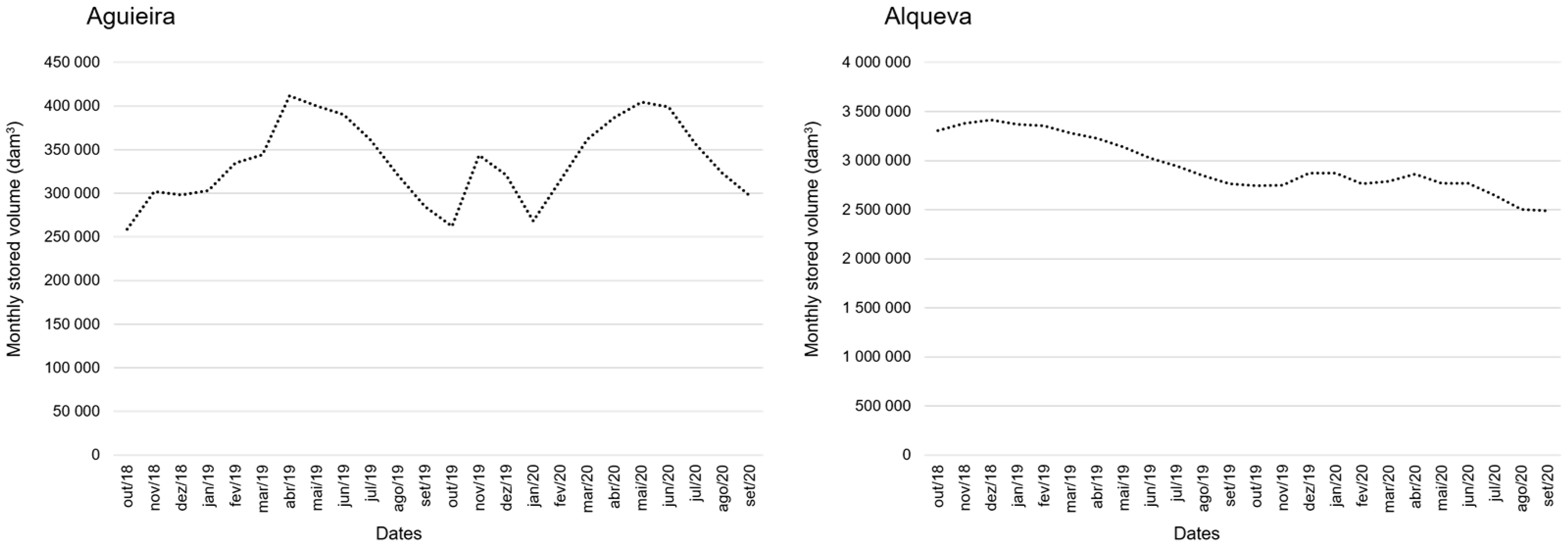
Figure A1.
Monthly mean stored volume of water in Aguieira reservoir (left) and Alqueva Reservoir (right), for the last two water years (2018–2019 ad 2019–2020) [44].
Figure A1.
Monthly mean stored volume of water in Aguieira reservoir (left) and Alqueva Reservoir (right), for the last two water years (2018–2019 ad 2019–2020) [44].

References
- Pekel, J.F.; Cottam, A.; Gorelick, N.; Belward, A.S. High-resolution mapping of global surface water and its long-term changes. Nature 2016, 540, 418–422. [Google Scholar] [CrossRef]
- Zhou, S.; Zhang, X.; Liu, J. The trend of small hydropower development in China. Renew. Energy 2009, 34, 1078–1083. [Google Scholar] [CrossRef]
- Corrigan, J.R.; Egan, K.J.; Downing, J.A. Aesthetic Values of Lakes and Rivers. In Encyclopedia of Inland Waters, 1st ed.; Likens, G.E., Ed.; Elsevier Science Publishers: Amsterdam, The Netherlands, 2009; pp. 14–24. [Google Scholar] [CrossRef]
- Corman, J. Cleaner Chinese lakes. Nat. Geosci. 2017, 10, 469–470. [Google Scholar] [CrossRef]
- Costanza, R.; D’Arge, R.; De Groot, R.; Farber, S.; Grasso, M.; Hannon, B.; Limburg, K.; Naeem, S.; O’Neill, R.V.; Paruelo, J.M.; et al. The value of the world’s ecosystem services and natural capital. Nature 1997, 387, 253–260. [Google Scholar] [CrossRef]
- Mishra, D.R.; Ogashawara, I.; Gitelson, A.A. Remote Sensing of Inland Waters: Background and Current State-of-the-Art. In Bio-Optical Modeling and Remote Sensing of Inland Waters, 1st ed.; Mishra, D.R., Ogashawara, I., Gitelson, A.A., Eds.; Elsevier Science Publishers: Amsterdam, The Netherlands, 2017; pp. 11–34. [Google Scholar]
- Scheffer, M.; Carpenter, S.R. Catastrophic regime shifts in ecosystems: Linking theory to observation. Trends Ecol. Evol. 2003, 18, 648–656. [Google Scholar] [CrossRef]
- European Community. Directive 2000/60/EC of the European Parliament and of the Council of 23 October 2000 establishing a framework for Community action in the field of water policy. Off. J. Eur. Parliam. 2000. [Google Scholar] [CrossRef]
- Blabolil, P.; Logez, M.; Ricard, D.; Prchalová, M.; Říha, M.; Sagouis, A.; Peterka, J.; Kubečka, J.; Argillier, C. An assessment of the ecological potential of Central and Western European reservoirs based on fish communities. Fish. Res. 2016, 173, 80–87. [Google Scholar] [CrossRef] [Green Version]
- Kampa, E.; Hansen, W. Definition of Maximum Ecological Potential. In Heavily Modified Waters in Europe: Synthesis of 34 Case Studies in Europe, 1st ed.; Springer: Berlin, Germany, 2004; pp. 137–152. [Google Scholar]
- Irz, P.; Laurent, A.; Messad, S.; Pronier, O.; Argillier, C. Influence of site characteristics on fish community patterns in French reservoirs. Ecol. Freshw. Fish 2002, 11, 123–136. [Google Scholar] [CrossRef]
- Wetzel, R.G. Rivers and Lakes—Their distribution, origins and forms. In Limnology: Lake and River Ecosystems, 3rd ed.; Elsevier Science Publishers: Amsterdam, The Netherlands, 2001; pp. 15–42. [Google Scholar]
- Ansper, A.; Alikas, K. Retrieval of Chlorophyll a from Sentinel-2 MSI Data for the European Union Water Framework Directive Reporting Purposes. Remote Sens. 2019, 11, 64. [Google Scholar] [CrossRef] [Green Version]
- Carvalho, L.; Mackay, E.B.; Cardoso, A.C.; Baattrup-Pedersen, A.; Birk, S.; Blackstock, K.L.; Borics, G.; Borja, A.; Feld, C.K.; Ferreira, M.T.; et al. Protecting and restoring Europe’s waters: An analysis of the future development needs of the Water Framework Directive. Sci. Total Environ. 2019, 658, 1228–1238. [Google Scholar] [CrossRef]
- Danovaro, R.; Carugati, L.; Berzano, M.; Cahill, A.E.; Carvalho, S.; Chenuil, A.; Corinaldesi, C.; Cristina, S.; David, R.; Dell’Anno, A.; et al. Implementing and Innovating Marine Monitoring Approaches for Assessing Marine Environmental Status. Front. Mar. Sci. 2016, 3, 3–213. [Google Scholar] [CrossRef]
- Tyler, A.; Hunter, P.D.; Spyrakos, E.; Groom, S.; Constantinescu, A.M.; Kitchen, J. Developments in Earth observation for the assessment and monitoring of inland, transitional, coastal and shelf-sea waters. Sci. Total Environ. 2016, 572, 1307–1321. [Google Scholar] [CrossRef] [PubMed] [Green Version]
- Gordon, H.R.; Brown, O.; Evans, R.H.; Brown, J.W.; Smith, R.C.; Baker, K.S.; Clark, D.K. A semianalytic radiance model of ocean color. J. Geophys. Res. Space Phys. 1988, 93, 10909–10924. [Google Scholar] [CrossRef]
- Morel, A.Y.; Gordon, H.R. Report of the working group on water color. Bound.-Layer Meteorol. 1980, 18, 343–355. [Google Scholar] [CrossRef]
- Morel, A. Bio-optical Models. In Encyclopedia of Ocean Sciences, 1st ed.; John, H.S., Ed.; Elsevier Science Publishers: Amsterdam, The Netherlands, 2001; pp. 317–326. [Google Scholar] [CrossRef]
- Preisendorfer, R.W. Hydrologic Optics. Environ. Res. 1976, 1, 392. [Google Scholar]
- Giardino, C.; Bresciani, M.; Stroppiana, D.; Oggioni, A.; Morabito, G. Optical remote sensing of lakes: An overview on Lake Maggiore. J. Limnol. 2014, 73, 201–214. [Google Scholar] [CrossRef] [Green Version]
- Drusch, M.; Del Bello, U.; Carlier, S.; Colin, O.; Fernandez, V.; Gascon, F.; Hoersch, B.; Isola, C.; Laberinti, P.; Martimort, P.; et al. Sentinel-2: ESA’s Optical High-Resolution Mission for GMES Operational Services. Remote Sens. Environ. 2012, 120, 25–36. [Google Scholar] [CrossRef]
- Donlon, C.; Berruti, B.; Buongiorno, A.; Ferreira, M.-H.; Féménias, P.; Frerick, J.; Goryl, P.; Klein, U.; Laur, H.; Mavrocordatos, C.; et al. The Global Monitoring for Environment and Security (GMES) Sentinel-3 mission. Remote Sens. Environ. 2012, 120, 37–57. [Google Scholar] [CrossRef]
- Ingmann, P.; Veihelmann, B.; Langen, J.; Lamarre, D.; Stark, H.; Courrèges-Lacoste, G.B. Requirements for the GMES Atmosphere Service and ESA’s implementation concept: Sentinels-4/-5 and -5p. Remote Sens. Environ. 2012, 120, 58–69. [Google Scholar] [CrossRef]
- Torres, R.; Snoeij, P.; Geudtner, D.; Bibby, D.; Davidson, M.; Attema, E.; Potin, P.; Rommen, B.; Floury, N.; Brown, M.; et al. GMES Sentinel-1 mission. Remote Sens. Environ. 2012, 120, 9–24. [Google Scholar] [CrossRef]
- Sentinel-2-Missions-Sentinel Online–Sentinel. Available online: https://sentinel.esa.int/web/sentinel/missions/sentinel-2 (accessed on 28 May 2021).
- Brockmann, C.; Doerffer, R.; Peters, M.; Stelzer, K.; Embacher, S.; Ruescas, A. Evolution of the C2RCC neural network for Sentinel 2 and 3 for the retrieval of ocean colour products in normal and extreme optically complex waters. Eur. Space Agency 2016, 740, 54. [Google Scholar]
- Matthews, M.W. A current review of empirical procedures of remote sensing in inland and near-coastal transitional waters. Int. J. Remote Sens. 2011, 32, 6855–6899. [Google Scholar] [CrossRef]
- Shanmugam, P. CAAS: An atmospheric correction algorithm for the remote sensing of complex waters. Ann. Geophys. 2012, 30, 203–220. [Google Scholar] [CrossRef]
- Topp, S.N.; Pavelsky, T.M.; Jensen, D.; Simard, M.; Ross, M.R.V. Research Trends in the Use of Remote Sensing for Inland Water Quality Science: Moving Towards Multidisciplinary Applications. Water 2020, 12, 169. [Google Scholar] [CrossRef] [Green Version]
- Modabberi, A.; Noori, R.; Madani, K.; Ehsani, A.H.; Mehr, A.D.; Hooshyaripor, F.; Kløve, B. Caspian Sea is eutrophying: The alarming message of satellite data. Environ. Res. Lett. 2020, 15, 124047. [Google Scholar] [CrossRef]
- Sòria-Perpinyà, X.; Urrego, P.; Pereira-Sandoval, M.; Ruiz-Verdú, A.; Peña, R.; Soria, J.M.; Moreno, J. Monitoring the ecological state of a hypertrophic lake (Albufera of València, Spain) using multitemporal Sentinel-2 images. Limnetica 2019, 38, 457–469. [Google Scholar] [CrossRef]
- Potes, M.; Rodrigues, G.; Penha, A.M.; Novais, M.H.; Costa, M.J.; Salgado, R.; Morais, M.M. Use of Sentinel 2–MSI for water quality monitoring at Alqueva reservoir, Portugal. Proc. Int. Assoc. Hydrol. Sci. 2018, 380, 73–79. [Google Scholar] [CrossRef]
- Duan, H.; Ma, R.; Xu, J.; Zhang, Y.; Zhang, B. Comparison of different semi-empirical algorithms to estimate chlorophyll-a concentration in inland lake water. Environ. Monit. Assess. 2010, 170, 231–244. [Google Scholar] [CrossRef]
- Hadjimitsis, D.G.; Clayton, C. Assessment of temporal variations of water quality in inland water bodies using atmospheric corrected satellite remotely sensed image data. Environ. Monit. Assess. 2009, 159, 281–292. [Google Scholar] [CrossRef] [PubMed]
- APA. Plano de Ordenamento da Albufeira da Aguieira. Diário da República 2007. 1ª série–Nº 8 190, pp. 1–2. [CrossRef]
- INAG. Available online: https://sniambgeoviewer.apambiente.pt/GeoDocs/geoportaldocs/_Agua/DRH/MonitorizacaoAvaliacao/EstadoMassasAgua/ModelacaoQualidadeAgua_AAP/I_RelatorioModelacao_CasteloBode.pdf (accessed on 28 May 2021).
- Pinto, I.; Rodrigues, S.; Lage, O.; Antunes, S. Assessment of water quality in Aguieira reservoir: Ecotoxicological tools in addition to the Water Framework Directive. Ecotoxicol. Environ. Saf. 2021, 208, 111583. [Google Scholar] [CrossRef]
- Presidência do Conselho de Ministros. Resolução do Conselho de Ministros nº 186/2007. Diário Da República 2007, 1ª série–Nº 246.
- Geraldes, A.M.; Silva-Santos, P. Monitorização da comunidade zooplanctónica da albufeira da Aguieira (bacia do Mondego, Portugal): Que fatores a influenciam? Captar Ciênc. E Ambient. Para Todos 2011, 3, 12–23. [Google Scholar]
- Pedroso, N.M.; Sales-Luís, T.; Santos-Reis, M. Use of Aguieira dam by Eurasian otters in Central Portugal. Folia Zool 2007, 56, 365. [Google Scholar]
- Geraldes, A.M.A.; Pasupuleti, R.; Silva-Santos, P. Influence of Some Environmental Variables on the Zooplankton Community of Aguieira Reservoir (Iberian Peninsula, Portugal): Spatial and Temporal Trends. Asian J. Environ. Ecol. 2016, 1, 1–10. [Google Scholar] [CrossRef] [Green Version]
- Rodrigues, C.M.; Moreira, M.; Guimarães, R.C.; Potes, M. Reservoir evaporation in a Mediterranean climate: Comparing direct methods in Alqueva Reservoir, Portugal. Hydrol. Earth Syst. Sci. 2020, 24, 5973–5984. [Google Scholar] [CrossRef]
- SNIRH > Dados Sintetizados. Available online: https://snirh.apambiente.pt/index.php?idMain=1&idItem=1.3 (accessed on 28 May 2021).
- CLC 2018—Copernicus Land Monitoring Service. Available online: https://land.copernicus.eu/pan-european/corine-land-cover/clc2018 (accessed on 28 May 2021).
- Kottek, M.; Grieser, J.; Beck, C.; Rudolf, B.; Rubel, F. World Map of the Köppen-Geiger climate classification updated. Meteorol. Z. 2006, 15, 259–263. [Google Scholar] [CrossRef]
- APHA. Standard Methods for the Examination of Water and Wastewater, 17th ed.; American Public Health Association: Washington, DC, USA, 1989.
- Lorenzen, C.J. Determination of Chlorophyll And Pheo-Pigments: Spectrophotometric Equations. Limnol. Oceanogr. 1967, 12, 343–346. [Google Scholar] [CrossRef]
- Stramski, D.; Boss, E.; Bogucki, D.; Voss, K. The role of seawater constituents in light backscattering in the ocean. Prog. Oceanogr. 2004, 61, 27–56. [Google Scholar] [CrossRef]
- Copernicus Open Access Hub. Available online: https://scihub.copernicus.eu/dhus/#/home (accessed on 28 May 2021).
- ESA Sentinel Application Platform (SNAP) v8.0. Available online: http://step.esa.int (accessed on 22 July 2021).
- Hair, J.F.; Black, W.C.; Babin, B.J.; Anderson, R.E. Multivariate Data Analysis, 8th ed.; Cengage Learning: Boston, MA, USA, 2018. [Google Scholar]
- Kato, T. Prediction of photovoltaic power generation output and network operation. In Integration of Distributed Energy Resources in Power Systems: Implementation, Operation and Control, 1st ed.; Funabashi, T., Ed.; Elsevier Science Publishers: Amsterdam, The Netherlands, 2016; Volume 1, pp. 77–108. [Google Scholar] [CrossRef]
- R Core Team. R: A Language and Environment for Statistical Computing; R Foundation for Statistical Computing: Vienna, Austria, 2019; Available online: https://www.R-project.org/ (accessed on 28 May 2021).
- Palmer, S.; Kutser, T.; Hunter, P.D. Remote sensing of inland waters: Challenges, progress and future directions. Remote Sens. Environ. 2015, 157, 1–8. [Google Scholar] [CrossRef] [Green Version]
- Plowey, M.A. Multi-Scale Approach to Monitoring the Optically Complex Coastal Waters of the Baltic Sea: A comparison of Satellite, Mooring, and Ship-based Monitoring of Water Quality. Master’s Thesis, Stockholm University, Stockholm, Sweden, 2019. [Google Scholar]
- Kyryliuk, D.; Kratzer, S. Evaluation of sentinel-3A OLCI products derived using the case-2 regional coastcolour processor over the Baltic Sea. Sensors 2019, 19, 3609. [Google Scholar] [CrossRef] [Green Version]
- Johansen, R.; Beck, R.; Nowosad, J.; Nietch, C.; Xu, M.; Shu, S.; Yang, B.; Liu, H.; Emery, E.; Reif, M.; et al. Evaluating the portability of satellite derived chlorophyll-a algorithms for temperate inland lakes using airborne hyperspectral imagery and dense surface observations. Harmful Algae 2018, 76, 35–46. [Google Scholar] [CrossRef]
- Huang, C.; Shi, K.; Yang, H.; Li, Y.; Zhu, A.-X.; Sun, D.; Xu, L.; Zou, J.; Chen, X. Satellite observation of hourly dynamic characteristics of algae with Geostationary Ocean Color Imager (GOCI) data in Lake Taihu. Remote Sens. Environ. 2015, 159, 278–287. [Google Scholar] [CrossRef]
- Yacobi, Y.Z.; Gitelson, A.; Mayo, M. Remote sensing of chlorophyll in Lake Kinneret using highspectral-resolution radiometer and Landsat TM: Spectral features of reflectance and algorithm development. J. Plankton Res. 1995, 17, 2155–2173. [Google Scholar] [CrossRef] [Green Version]
- Pereira-Sandoval, M.; Ruescas, A.; Urrego, P.; Ruiz-Verdú, A.; Delegido, J.; Tenjo, C.; Soria-Perpinyà, X.; Vicente, E.; Soria, J.; Moreno, J. Evaluation of Atmospheric Correction Algorithms over Spanish Inland Waters for Sentinel-2 Multi Spectral Imagery Data. Remote Sens. 2019, 11, 1469. [Google Scholar] [CrossRef] [Green Version]
- Toming, K.; Kutser, T.; Uiboupin, R.; Arikas, A.; Vahter, K.; Paavel, B. Mapping Water Quality Parameters with Sentinel-3 Ocean and Land Colour Instrument imagery in the Baltic Sea. Remote Sens. 2017, 9, 1070. [Google Scholar] [CrossRef] [Green Version]
- Mishra, D.R.; Ogashawara, I.; Gitelson, A.A. Atmospheric Correction for Inland Waters. In Bio-Optical Modeling and Remote Sensing of Inland Waters, 1st ed.; Mishra, D.R., Ogashawara, I., Gitelson, A.A., Eds.; Elsevier Science Publishers: Amsterdam, The Netherlands, 2017; pp. 78–109. [Google Scholar]
- Nilsson, C. Reservoirs. In Encyclopedia of Inland Waters, 1st ed.; Nilsson, C., Ed.; Elsevier Science Publishers: Amsterdam, The Netherlands, 2009; pp. 625–633. [Google Scholar] [CrossRef]
- EVDC. Available online: https://evdc.esa.int/orbit/ (accessed on 28 May 2021).
- Downing, J.A. Limnology and oceanography: Two estranged twins reuniting by global change. Inland Waters 2014, 4, 215–232. [Google Scholar] [CrossRef] [Green Version]
- Diversity II. Available online: http://www.diversity2.info/ (accessed on 28 May 2021).
- eartH2Observe. Available online: http://www.earth2observe.eu/ (accessed on 28 May 2021).
- Brower, J.E.; Zar, J.H.; von Ende, C.N. Field and Laboratory Methods for General Ecology, 4th ed.; WCB McGraw-Hill: Boston, MA, USA, 1997. [Google Scholar]
- Williamson, C.E.; Morris, D.P.; Pace, M.L.; Olson, O.G. Dissolved organic carbon and nutrients as regulators of lake ecosystems: Resurrection of a more integrated paradigm. Limnol Oceanogr 1999, 44, 795–803. [Google Scholar] [CrossRef] [Green Version]
Figure 1.
Reservoirs’ locations within Portugal. Aguieira (A) reservoir sampling sites: A1 (40°0′7.942″ N, 8°11′38.616″ W), A2 (40°22′01.884″ N, 8°10’28.283″ W), A3 (40°24′03.488″ N, 8°07′01.150″ W), and A4 (40°22′22.256″ N, 8°03′19.055″ W); and Alqueva (Al) reservoir sampling sites: Al1 (38°12′07.957″ N, 7°29′19.717″ W), Al2 (38°17′35.785″ N, 7°33′41.484″ W), Al3 (38°25′58.085″ N, 7°21′03.721″ W), Al4 (38°32′49.092″ N, 7°18′13.988″ W), and Al5 (38°44′15.763″ N, 7°14′15.144″ W).

Figure 2.
Schematic representation of the workflow used for image processing and output achievement.
Figure 2.
Schematic representation of the workflow used for image processing and output achievement.

Figure 3.
PCA of in-situ data from both reservoirs. O2 is oxygen concentration (mg L−1), Cond is Conductivity (μS cm−1), TSS is total suspended solids measured in situ (mg L−1), Chl a is the chlorophyll a measured in situ (μg L−1), BOD5 is the five-days biochemical oxygen demand (mg L−1), VSS is the volatile suspended solids (mg L−1), Turb is the turbidity (m), DOC is the dissolved organic carbon (m−1), TH is the title hydrometric (°f), Fe is iron (μg L−1), Mn is manganese (μg L−1), As is arsenic (μg L−1), NH4 is ammonium (mg L−1), N is Kjedahl nitrogen (mg L−1), and P is Phosphorus (mg L−1).

Figure 4.
Scatter plots between in-situ data of chlorophyll a (μg L−1) and total suspended solids (mg L−1) in (a) Aguieira and (b) Alqueva.
Figure 4.
Scatter plots between in-situ data of chlorophyll a (μg L−1) and total suspended solids (mg L−1) in (a) Aguieira and (b) Alqueva.

Figure 5.
(a) Correlation between in situ and SNAP-C2RCC chlorophyll a values; (b) Correlation between in situ total suspended solids and SNAP-C2RCC total suspended solids values; a dashed X = Y line is also presented in each plot.
Figure 5.
(a) Correlation between in situ and SNAP-C2RCC chlorophyll a values; (b) Correlation between in situ total suspended solids and SNAP-C2RCC total suspended solids values; a dashed X = Y line is also presented in each plot.

Figure 6.
Correlation between (a) in situ and SNAP-C2RCC chlorophyll a values and (b) in situ total suspended solids and SNAP-C2RCC total suspended solids values for the Alqueva reservoir, using the 60 m product. Normalized root mean squared error (NRMSE), normalized mean bias error (NMBE), number of observations (n) and dashed X = Y lines are also presented.

Table 1.
Match-ups between sampling dates and satellite imagery dates.
| Reservoir | Data Source | Autumn 2018 | Spring 2019 | Autumn 2019 | Spring 2020 |
|---|---|---|---|---|---|
| Aguieira | In situ | 5–7 October | 6 April | 12 November | 10 May |
| Satellite | 7 October | 31 March | - | 19 May | |
| Alqueva | In situ | 16 November | 15 May | 18 November | 27 May |
| Satellite | 16 November | 15 May | 18 November | 26 May |
Table 2.
Results from laboratory analysis and image processing using SNAP-C2RCC, concerning the Chl a and TSS parameters. “Chl a” is the measurement in situ (μg L−1) and “Chl-S20m” and “Chl-S60m” are the SNAP-C2RCC estimated variables for chlorophyll a (μg L−1), using the 20 m and 60 m products, respectively. “TSS” is the measurement in situ (mg L−1) and “TSS-S20m” and “TSS-S60m” are the SNAP-C2RCC estimated variables for total suspended solids (mg L−1), using the 20 m and 60 m products, respectively. Sites A1 to A4 belong to the Aguieira reservoir and Al1 to Al5 to the Alqueva reservoir.
| Season | Site | Chl a | Chl-S20m | Chl-S60m | TSS | TSS-S20m | TSS-S60m |
|---|---|---|---|---|---|---|---|
| Aut18 | A1 | 5.429 | 11.65 | 6.231 | 8.240 | 9.382 | 13.78 |
| A2 | 10.10 | 42.71 | 9.973 | 10.09 | 14.89 | 2.935 | |
| A4 | 3.438 | 6.816 | 3.699 | 10.75 | 21.66 | 8.598 | |
| Al1 | 0.980 | 8.982 | 0.993 | 4.280 | 1.607 | 2.322 | |
| Al2 | 3.596 | 1.654 | 1.958 | 3.830 | 1.874 | 2.683 | |
| Al3 | 1.812 | 2.044 | 7.387 | 4.720 | 6.625 | 4.746 | |
| Al4 | 2.183 | 4.125 | 0.799 | 3.610 | 24.51 | 4.196 | |
| Al5 | 31.26 | 5.474 | 15.45 | 15.42 | 24.84 | 23.94 | |
| Spr19 | A1 | 26.32 | 31.50 | 18.27 | 13.45 | 9.866 | 10.67 |
| A2 | 30.62 | 29.75 | 7.863 | 19.05 | 19.51 | 0.458 | |
| A4 | 27.90 | 12.18 | 4.131 | 17.50 | 24.25 | 1.163 | |
| Al1 | 2.285 | 3.513 | 4.082 | 7.750 | 1.607 | 9.045 | |
| Al2 | 0.936 | 0.425 | 0.908 | 7.420 | 1.874 | 7.560 | |
| Al3 | 2.494 | 2.005 | 6.839 | 7.420 | 6.625 | 11.79 | |
| Al4 | 7.832 | 5.023 | 6.564 | 12.75 | 24.51 | 13.83 | |
| Al5 | 56.65 | 27.16 | 63.41 | 20.42 | 24.84 | 19.49 | |
| Aut19 | Al1 | 3.534 | 3.813 | 6.839 | 10.02 | 10.62 | 11.19 |
| Al2 | 8.276 | 5.986 | 16.36 | 24.72 | 30.35 | 16.34 | |
| Al3 | 2.747 | 15.04 | 3.098 | 7.880 | 5.143 | 6.450 | |
| Al4 | 2.806 | 3.642 | 3.447 | 9.780 | 24.24 | 9.400 | |
| Al5 | 40.10 | 40.22 | 42.13 | 29.97 | 30.73 | 30.02 | |
| Spr20 | A1 | 26.16 | 0.800 | 0.577 | 15.19 | 0.183 | 0.030 |
| A2 | 42.08 | 2.663 | 0.259 | 17.542 | 3.063 | 0.018 | |
| A4 | 31.75 | 9.928 | 1.070 | 11.233 | 4.838 | 2.385 | |
| Al1 | 2.197 | 3.270 | 3.546 | 6.250 | 7.993 | 25.92 | |
| Al2 | 2.281 | 2.892 | 3.156 | 7.083 | 12.32 | 3.135 | |
| Al3 | 3.675 | 3.530 | 1.099 | 6.317 | 6.542 | 5.812 | |
| Al4 | 20.78 | 21.80 | 21.87 | 10.02 | 8.101 | 10.41 | |
| Al5 | 45.42 | 49.37 | 49.54 | 28.50 | 9.931 | 19.20 |
Table 3.
Normalized root mean squared error (NRMSE) and the normalized mean bias error (NMBE) results for the two reservoirs.
Table 3.
Normalized root mean squared error (NRMSE) and the normalized mean bias error (NMBE) results for the two reservoirs.
| Reservoir | Parameter | 20 m Product | 60 m Product | |
|---|---|---|---|---|
| Chl a | NRMSE (%) | 55.0 | 57.8 | |
| Aguieira | NMBE (%) | −16.4 | −43.6 | |
| TSS | NRMSE (%) | 80.3 | 112 | |
| NMBE (%) | −15.8 | −85.3 | ||
| Chl a | NRMSE (%) | 16.7 | 8.9 | |
| Alqueva | NMBE (%) | −4.2 | 1.7 | |
| TSS | NRMSE (%) | 32 | 21.9 | |
| NMBE (%) | 7.2 | 2.0 |
Table 4.
Normalized root mean squared error (NRMSE) and the normalized mean bias error (NMBE) results for Aguieira, without observations from spring of 2020.
Table 4.
Normalized root mean squared error (NRMSE) and the normalized mean bias error (NMBE) results for Aguieira, without observations from spring of 2020.
| Reservoir | Parameter | 20 m Product | 60 m Product | |
|---|---|---|---|---|
| Chl a | NRMSE (%) | 56.0 | 50.9 | |
| Aguieira | NMBE (%) | 18.9 | −32.9 | |
| TSS | NRMSE (%) | 53.7 | 100.4 | |
| NMBE (%) | 31.6 | −64.0 |
Publisher’s Note: MDPI stays neutral with regard to jurisdictional claims in published maps and institutional affiliations. |
© 2021 by the authors. Licensee MDPI, Basel, Switzerland. This article is an open access article distributed under the terms and conditions of the Creative Commons Attribution (CC BY) license (https://creativecommons.org/licenses/by/4.0/).
Share and Cite
MDPI and ACS Style
Neves, V.H.; Pace, G.; Delegido, J.; Antunes, S.C. Chlorophyll and Suspended Solids Estimation in Portuguese Reservoirs (Aguieira and Alqueva) from Sentinel-2 Imagery. Water 2021, 13, 2479. https://doi.org/10.3390/w13182479
AMA Style
Neves VH, Pace G, Delegido J, Antunes SC. Chlorophyll and Suspended Solids Estimation in Portuguese Reservoirs (Aguieira and Alqueva) from Sentinel-2 Imagery. Water. 2021; 13(18):2479. https://doi.org/10.3390/w13182479
Chicago/Turabian StyleNeves, Vítor Hugo, Giorgio Pace, Jesús Delegido, and Sara C. Antunes. 2021. "Chlorophyll and Suspended Solids Estimation in Portuguese Reservoirs (Aguieira and Alqueva) from Sentinel-2 Imagery" Water 13, no. 18: 2479. https://doi.org/10.3390/w13182479
Note that from the first issue of 2016, this journal uses article numbers instead of page numbers. See further details here.