
Optimization-Based Proposed Solution for Water Shortage Problems: A Case Study in the Ismailia Canal, East Nile Delta, Egypt

 ,
,  , and
, and 
Abstract
:1. Introduction
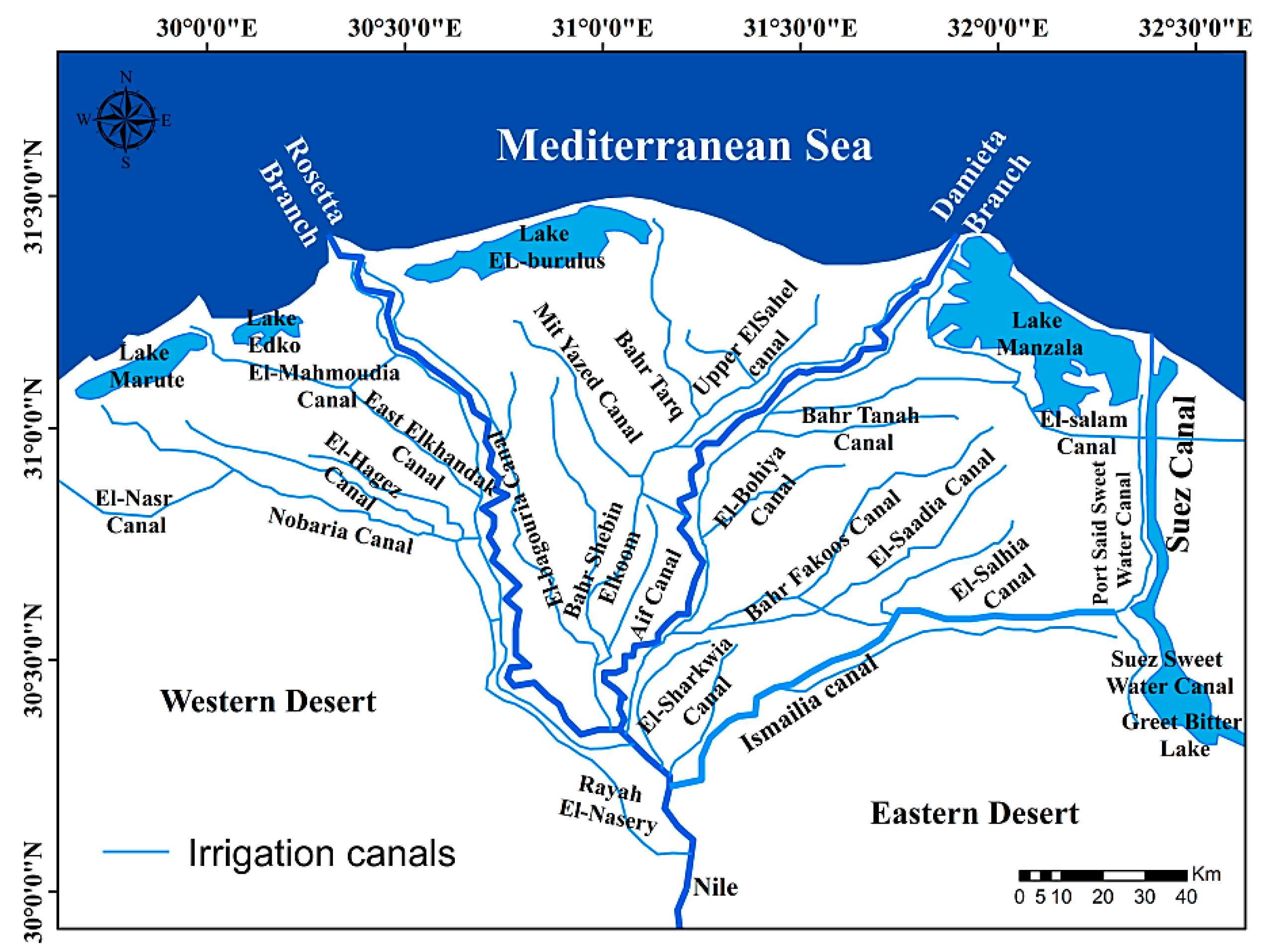
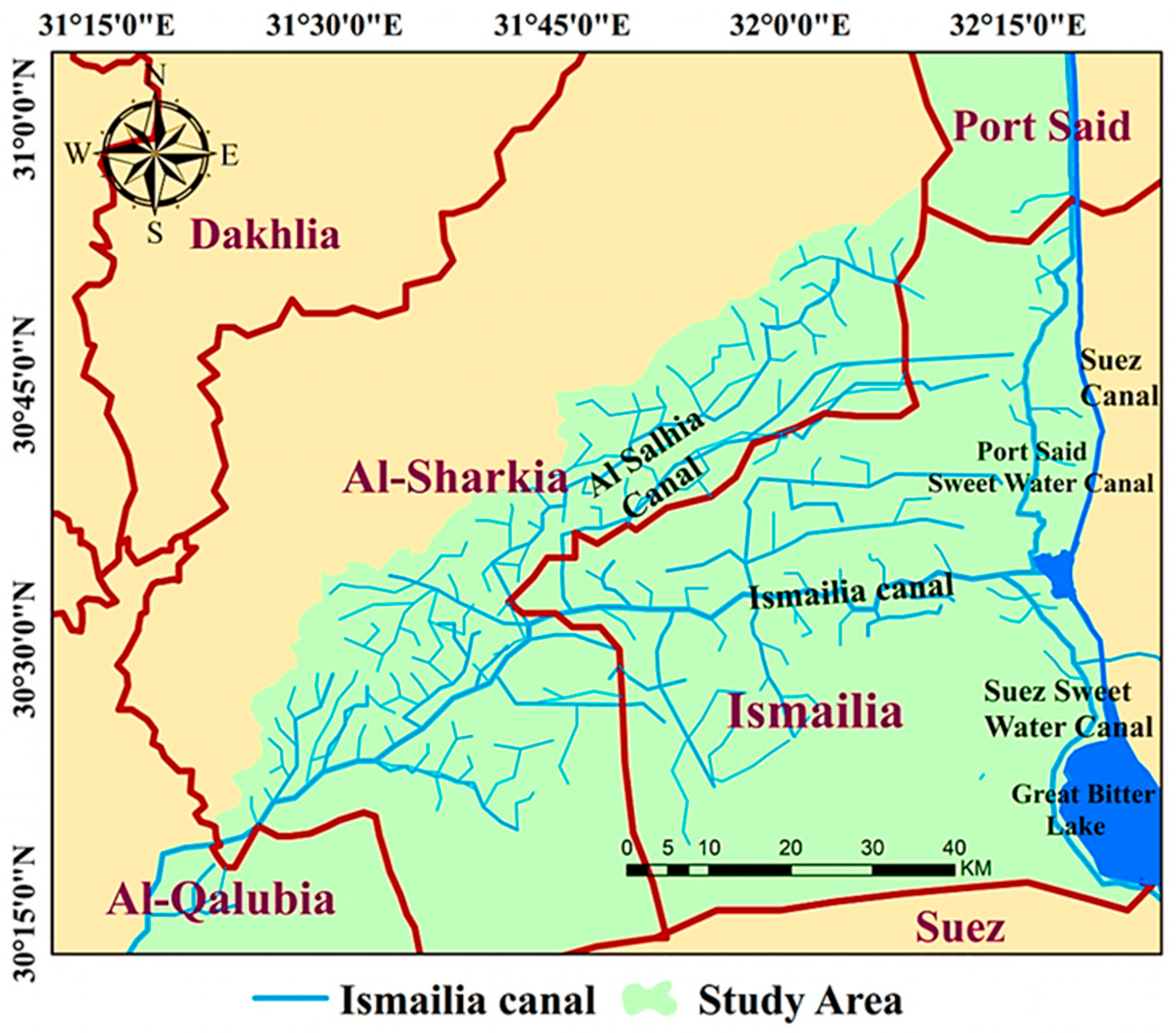
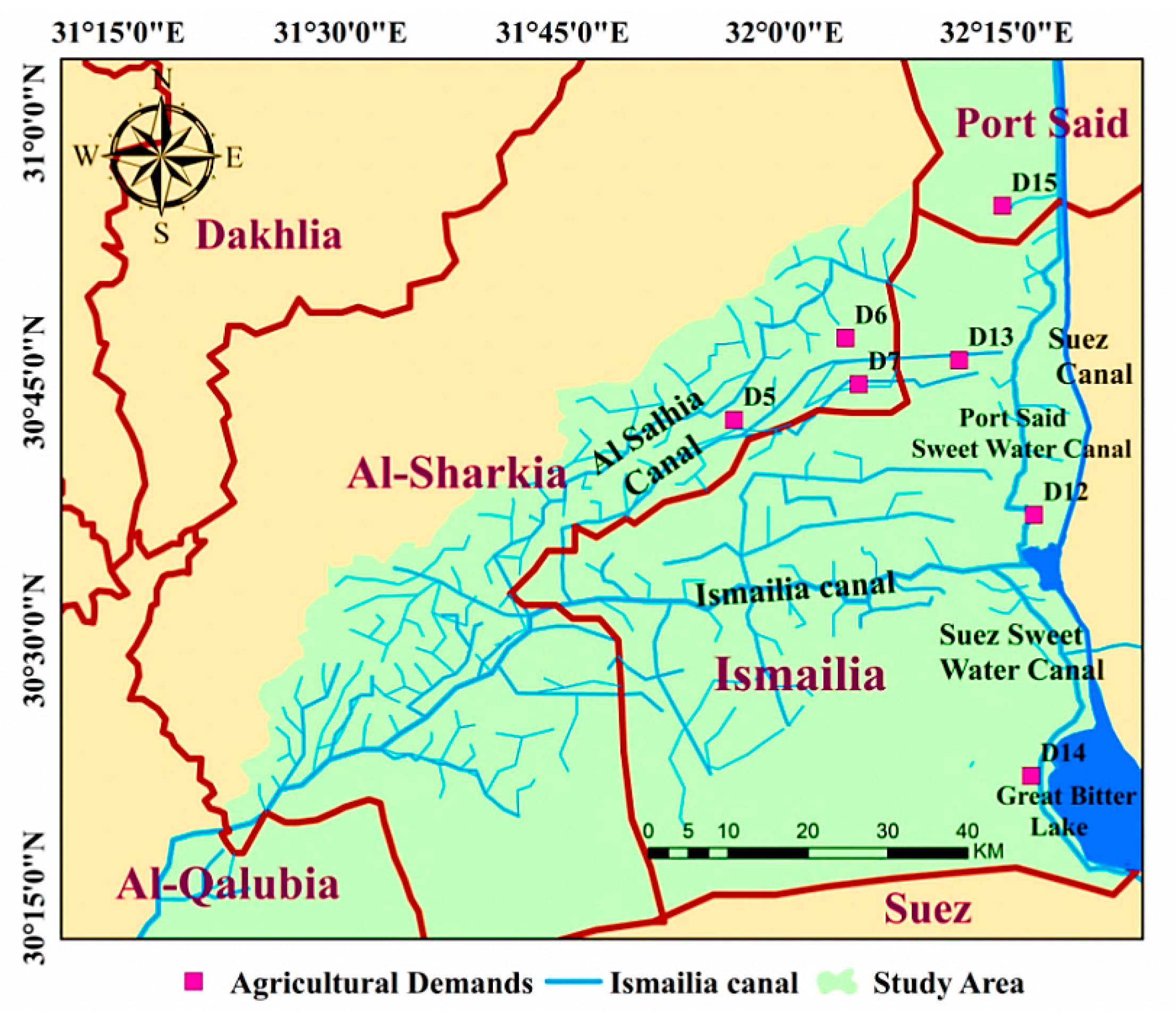
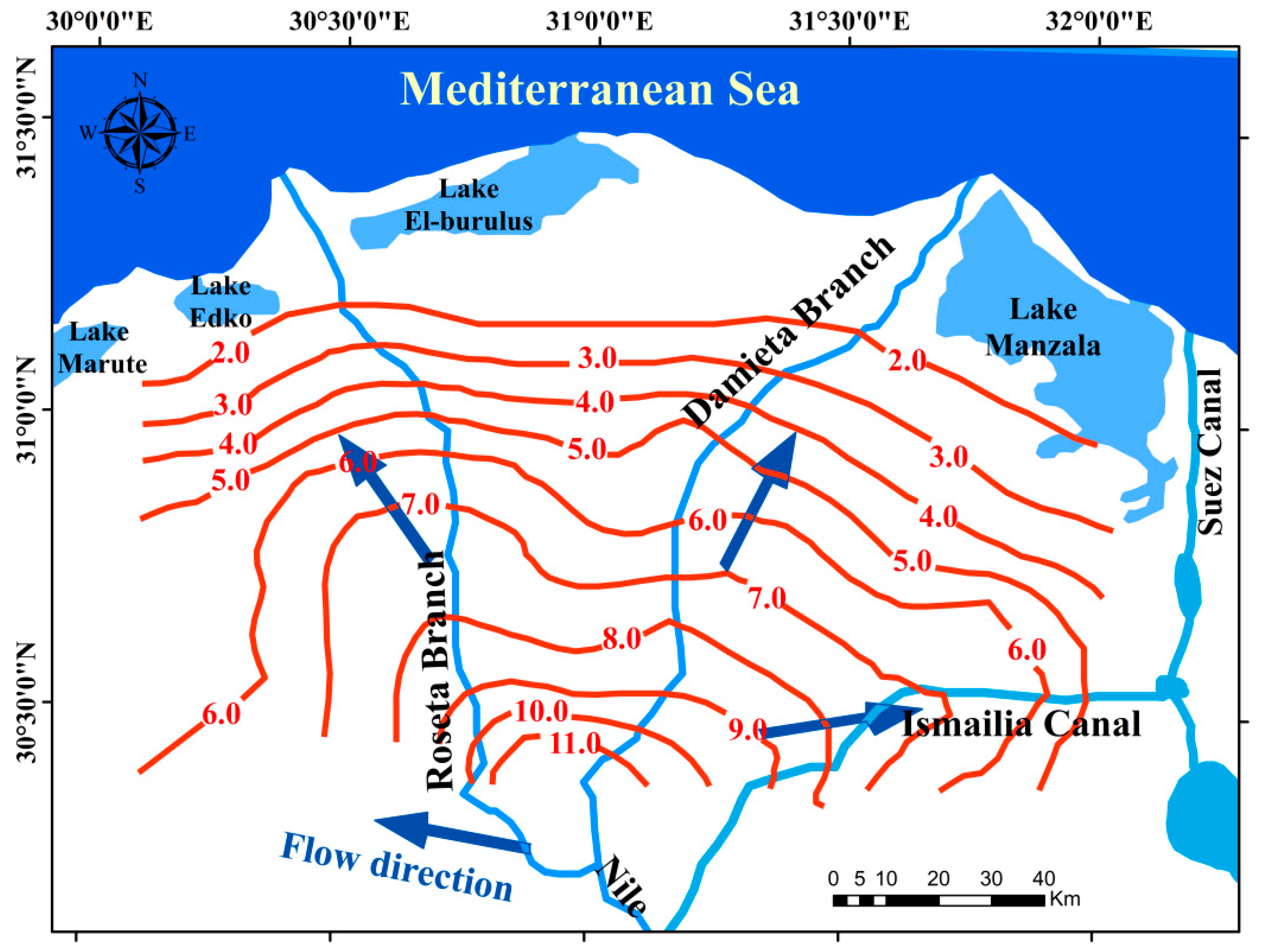
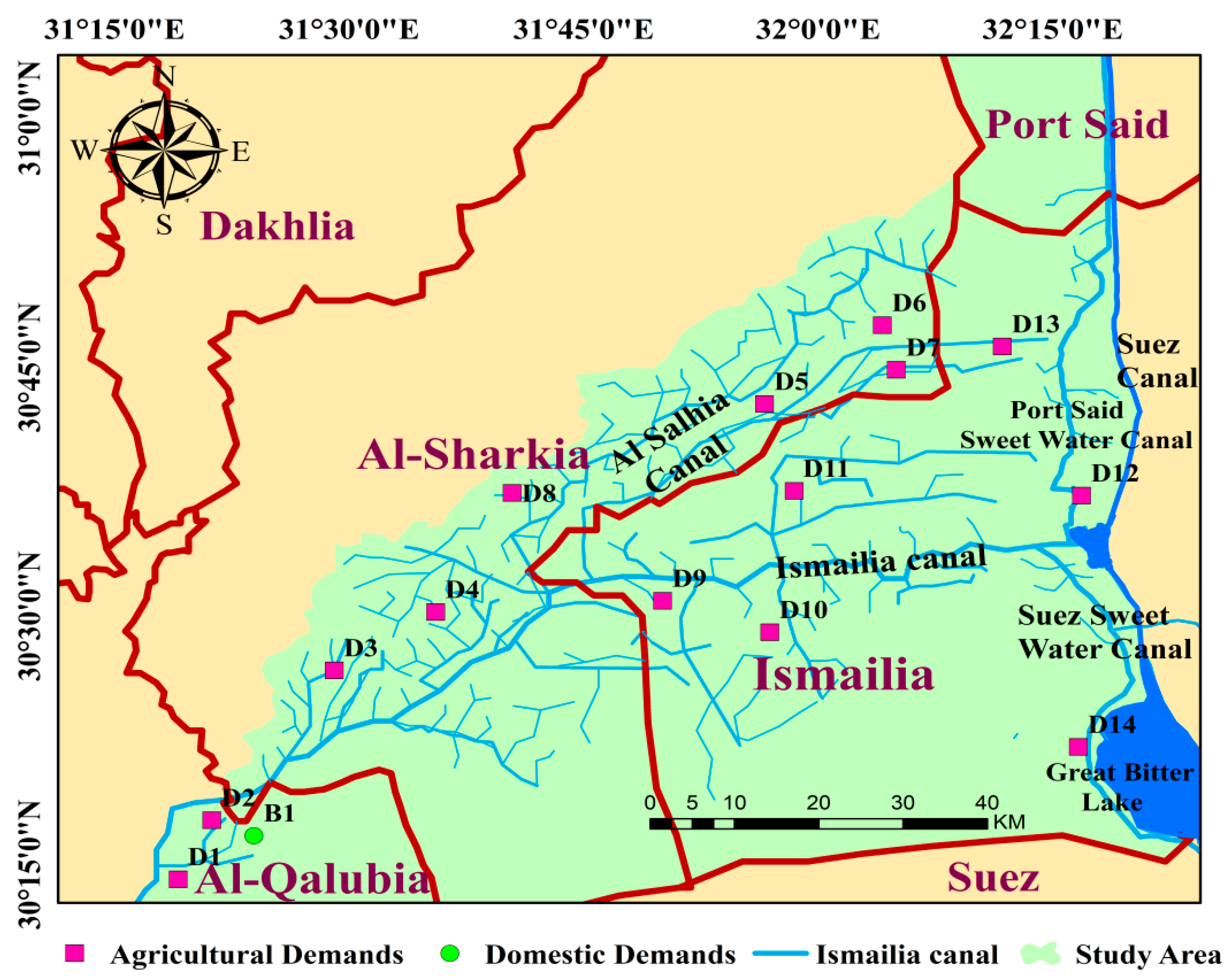
2. Physical Conditions for the Study Area
3. Materials and Methods
3.1. Model Setup
3.1.1. Sets and Indices
- t: Time step (month)
- dem: Agricultural demands,
- sr: Surface water sources,
- booster: Domestic demands,
- gw: Groundwater sources
- ru: Reuse water sources
3.1.2. Data Sets
- Supply characteristics
- 2.
- Demand characteristics
3.1.3. Variables
- : Discharge from the canal to agricultural demand area “dem” in time step “t”
- : Discharge from the canal to domestic demand site “booster” in time step “t”
- : Groundwater pumped to agricultural demand area “dem” in time step “t”
- : Groundwater pumped to domestic demand site “booster” in time step “t”
- : Reuse water pumped to agricultural demand area “dem” in time step “t”
- : The ratio of water supply to domestic demand site “booster” in time step “t”
- : Water shortage between water supply and demands at agricultural demand area “dem” in time step “t”.
3.1.4. Objective Functions
3.1.5. Model Constraints
- 1.
- Water balance at agricultural demand area “dem” in time step “t”.
- 2.
- Water balance at domestic demand site “booster” in time step “t”.
- 3.
- Surface water source limit in time step “t”.
- 4.
- Ratio of water supply to domestic demand site.
- 5.
- Groundwater source limit.
- 6.
- Reuse water source limit.
3.2. LINDO Software
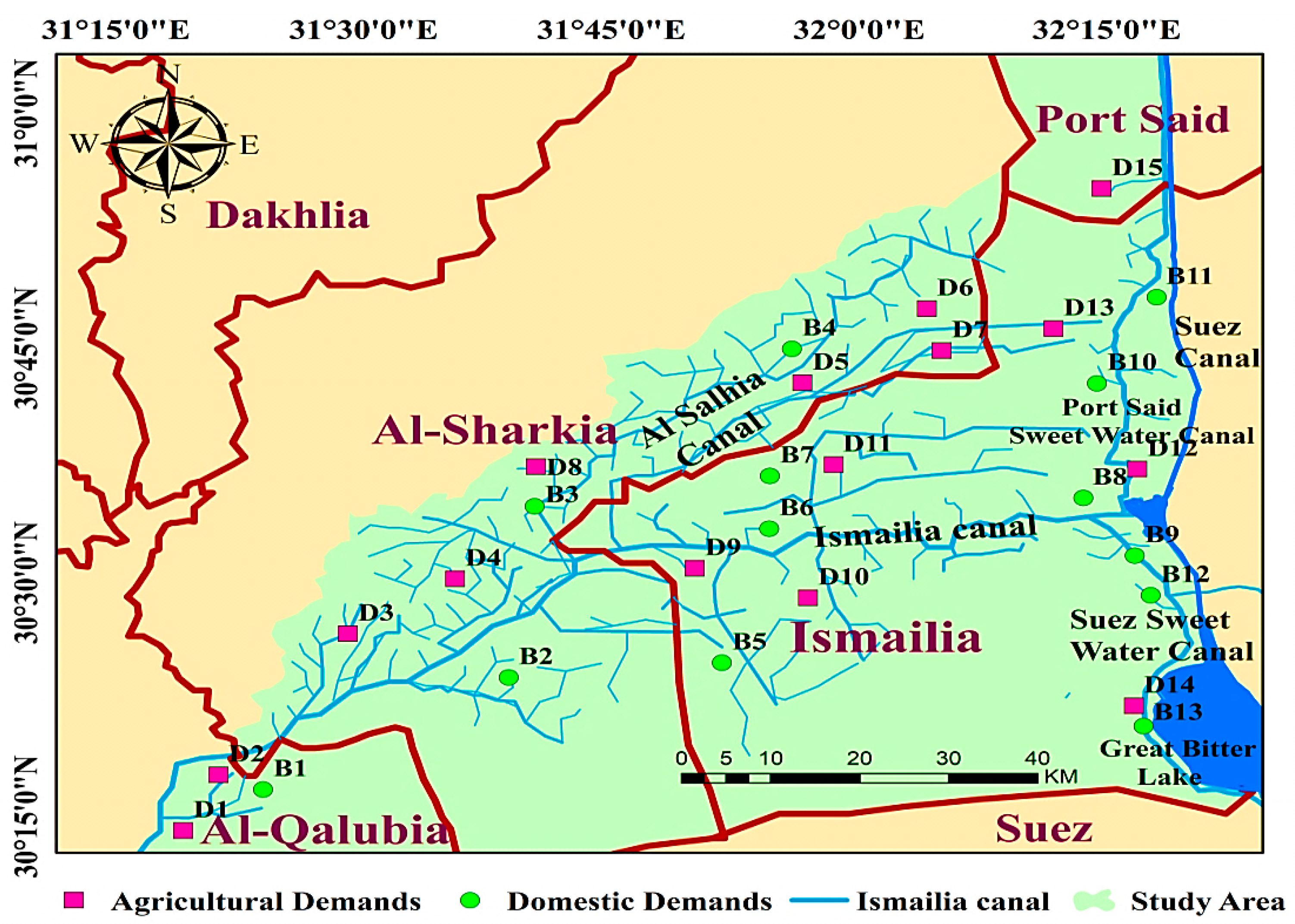
3.3. Model Development
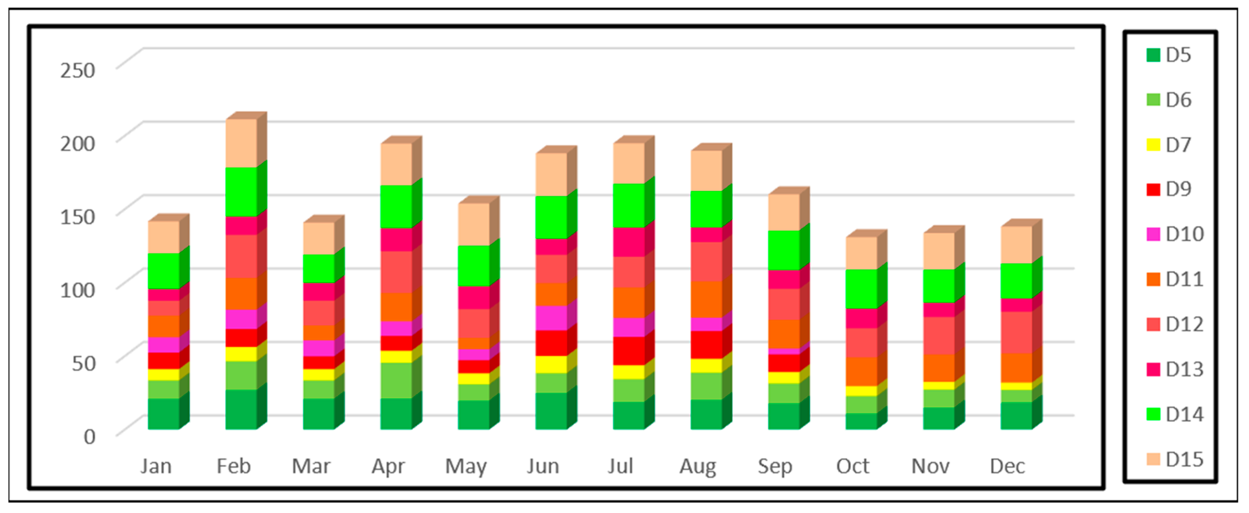
- Water demands: agriculture land (15 demand nodes) and Al-Salhiya is the largest agricultural region in the study area, with 118,371 Feddan, so the area was divided into three demand nodes at the end of the Salhia canal network (D5, D6, D7), drinking purifications (13 boosters) and seepage is about 21.06% of the total discharge [50].
4. Results and Discussion
4.1. Base Case
4.2. The Impact of Lining the Ismailia Canal
4.2.1. Lining Three Reaches with a Total Length of 57 km
4.2.2. Lining Four Reaches with a Total Length of 61 Km
4.3. The Impact of Surface Water
4.3.1. Increased Water Surface of the Ismailia Canal by 15%
4.3.2. Decrease in Ismailia Canal Head Flow by 10%
4.3.3. Use Surface-Water Only from the Ismailia Canal
4.4. The Impact of Groundwater
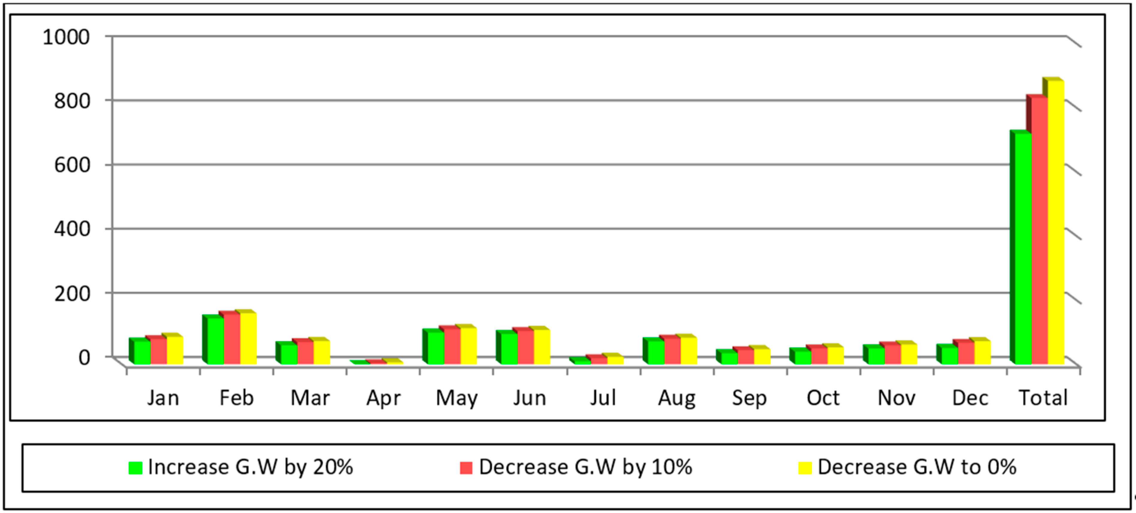
- Where the use of groundwater is increased by 20%, the unmet demand decreases from 789.81 to 718.7 MCM/year;
- By decreasing by 10%, the unmet demand increases from 789.81 to 829.4 MCM/year; and
- Using Surface water and reuse water only (without using any groundwater), results in the unmet demand increasing from 789.81 to 883.48 MCM/year.
5. Conclusions
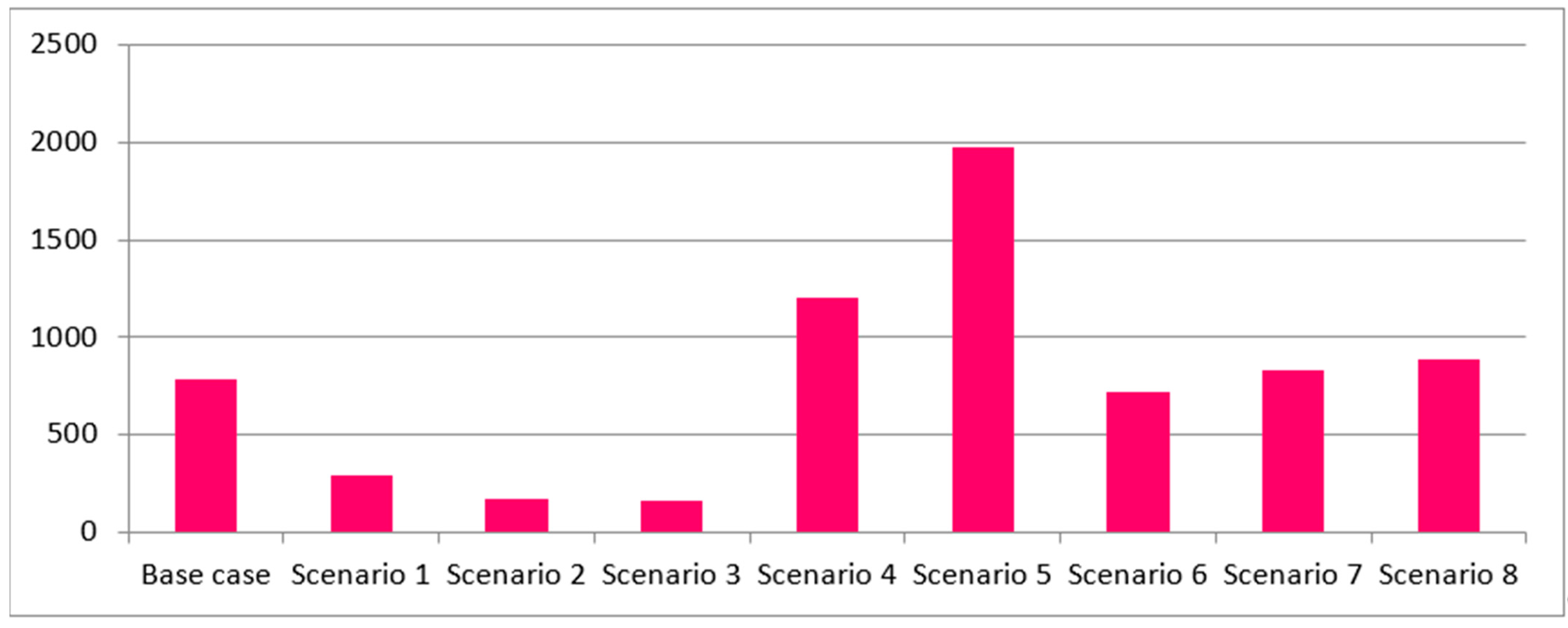
- Lining the Ismailia Canal results in an inverse proportion with the water scarcity value, reduced seepage from 21.06 percent to 10.16 percent, and a lowered water shortage, from 789.81 MCM to 291.99 MCM. Lining three sections of the canal reduced seepage from 21.06 percent to 7.51 percent, and lowered the water shortage from 789.81 MCM to 173.9 MCM;
- When the surface water of the Ismailia Canal is increased by 15%, water shortage decreases to 159.8 MCM/year, but when the surface water of the Ismailia Canal is decreased by 10%, water shortage increases to 1199.16 MCM/year. When relying on surface water without groundwater and reusing water, the shortage increases to 159.8 MCM/year; and,
- The value of a water shortage is inversely proportional to the amount of groundwater available. For example, increasing the groundwater by 20% reduces the water shortage to 718.7 MCM/year. However, if groundwater is reduced by 10%, the water deficit rises to 829.40 MCM/year. When relying on surface water and reusing it instead of groundwater, the annual shortage rises to 883.48 MCM.
6. Recommendations
- It is essential to create a locally comprehensive optimization model to include operational guidance that takes into account the various management variables, as well as the surface and groundwater salt balance to achieve optimum operation;
- In future research, evaporation and precipitation modes should be taken into account;
- Research on the effects of climate change on water supply and demand;
- Economic factors influencing water resources, as a result of GIS studies;
- Raising citizen consciousness is a good idea;
- Increasing the number of treatment plants to reduce waste; and
- Using cutting-edge irrigation and land-leveling technologies.
Author Contributions
Funding
Institutional Review Board Statement
Informed Consent Statement
Data Availability Statement
Acknowledgments
Conflicts of Interest
References
- UN-Water, FAO. Coping with Water Scarcity. Challenge of the Twenty-First Century; UN-Water, FAO: Rome, Italy, 2007; Available online: http://www.fao.org/3/a-aq444e.pdf (accessed on 15 May 2021).
- WHO (World Health Organization). Environmental Health Eastern Mediterranean Regional; Center for Environmental Health Activities (CEHA): Amman, Jordan, 2002. [Google Scholar]
- Sisira Saddhamangala Withanachchi. The Study of Transboundary Groundwater Governance in the Notion of Governmen-tality: In the Case of Guaraní Aquifer. AQUA Mundi. 2012. Available online: https://www.ssoar.info/ssoar/bitstream/handle/document/34939/ssoar-aqua-2012-6-withanachchi-The_study_of_Transboundary_Groundwater.pdf?sequence=1&isAllowed=y&lnkname=ssoar-aqua-2012-6-withanachchi-The_study_of_Transboundary_Groundwater.pdf (accessed on 19 August 2021).
- Kibaroğlu, A. Water diplomacy frameworks in the Middle East and the Euphrates-Tigris river basin. In Annual Conference IEMed; European Institute of the Mediterranean (IEMed): Barcelona, Spain, 2020. [Google Scholar]
- Kibaroğlu, A. Water Diplomacy Frameworks in the Euphrates–Tigris River Basin: A Theoretical Analysis. In Proceedings of the Conference on Transboundary Waters in International Relations, Mixing Water and International Relations Theory: Frameworks for Transboundary Water Analysis, Budapest, Hungary, 26–28 April 2021. [Google Scholar]
- Allam, A.; Fliefle, A.; Tawfik, A.; Yoshimura, Y.; El Saadi, A. A simulation-based suitability index of the quality and quantity of agricultuarla drainage water for reuse in irrigation. Sci. Total Environ. 2015, 536, 79–90. [Google Scholar] [CrossRef] [PubMed]
- FAO. Water and Agriculture in the Nile Basin. Nile Basin Initiative Report to ICCON; Background Paper Prepared by FAO; FAO: Rome, Italy, 2000. [Google Scholar]
- Varlet, M. Étude Graphique des Conditions d’Exploitation d’un Réservoir de Régularisation. Ann. Ponts Chaussées Partie Technol. 1923, 2, 93. [Google Scholar]
- Molinos-Senante, M.; Hernández-Sancho, F.; Mocholí-Arce, M.; Sala-Garrido, R. A management and optimisation model for water supply planning in water deficit areas. J. Hydrol. 2014, 515, 139–146. [Google Scholar] [CrossRef]
- Alizadeh, H.; Mousavi, S.J.; Ponnambalam, K. Copula-Based Chance-Constrained Hydro-Economic Optimization Model for Optimal Design of Reservoir-Irrigation District Systems under Multiple Interdependent Sources of Uncertainty. Water Resour. Res. 2018, 54, 5763–5784. [Google Scholar] [CrossRef]
- Guariso, G.; Whittington, D. Implications of ethiopian water development for Egypt and Sudan. Int. J. Water Resour. Dev. 1987, 3, 105–114. [Google Scholar] [CrossRef]
- Whittington, D.; Wu, X.; Sadoff, C. Water resources management in the Nile basin: The economic value of cooperation. Hydrol. Res. 2005, 7, 227–252. [Google Scholar] [CrossRef]
- Goor, Q.; Halleux, C.; Mohamed, Y.; Tilmant, A. Optimal operation of a multipurpose multireservoir system in the Eastern Nile River Basin. Hydrol. Earth Syst. Sci. 2010, 14, 1895–1908. [Google Scholar] [CrossRef] [Green Version]
- Arjoon, D.; Mohamed, Y.; Goor, Q.; Tilmant, A. Hydro-economic risk assessment in the eastern Nile River basin. Water Resour. Econ. 2014, 8, 16–31. [Google Scholar] [CrossRef]
- Lee, Y.; Yoon, T.; Shah, F.A. Optimal Watershed Management for Reservoir Sustainability: Economic Appraisal. J. Water Resour. Plan. Manag. 2012, 139, 129–138. [Google Scholar] [CrossRef]
- Attia, B. Inundations by High Releases Downstream High Aswan Dam. Nile Water Sci. Eng. J. 2010, 3, 2. [Google Scholar]
- Elnashar, W.Y. Groundwater Management in Egypt. IOSR J. Mech. Civ. Eng. 2014, 11, 69–78. [Google Scholar] [CrossRef] [Green Version]
- Ruiz-Rosa, I.; García-Rodríguez, F.J.; Jimenez, J.M. Development and application of a cost management model for wastewater treatment and reuse processes. J. Clean. Prod. 2016, 113, 299–310. [Google Scholar] [CrossRef]
- Al-Zahrani, M.; Musa, A.; Chowdhury, S. Multi-objective optimization model for water resource management: A case study for Riyadh, Saudi Arabia. Environ. Dev. Sustain. 2016, 18, 777–798. [Google Scholar] [CrossRef]
- Atilhan, S.; Mahfouz, A.B.; Batchelor, B.; Linke, P.; Abdel-Wahab, A.; Nápoles-Rivera, F.; Jiménez-Gutiérrez, A.; El-Halwagi, M.M. A systems-integration approach to the optimization of macroscopic water desalination and distribution networks: A general framework applied to Qatar’s water resources. Clean Technol. Environ. Policy 2011, 14, 161–171. [Google Scholar] [CrossRef]
- Elbeih, S. An overview of integrated remote sensing and GIS for groundwater mapping in Egypt. Ain Shams Eng. J. 2015, 6, 1–15. [Google Scholar] [CrossRef] [Green Version]
- El-Rawy, M.; Fathi, H.; Abdalla, F. Integration of remote sensing data and in situ measurements to monitor the water quality of the Ismailia Canal, Nile Delta, Egypt. Environ. Geochem. Health 2020, 42, 2101–2120. [Google Scholar] [CrossRef]
- Elewa, H.H.; Nosair, A.M.; Ramadan, E.M. Determination of Potential Sites and Methods for Water Harvesting in Sinai Peninsula by the Application of RS, GIS, and WMS Techniques; Springer Science and Business Media LLC: Berlin/Heidelberg, Germany, 2020; pp. 313–345. [Google Scholar]
- Jha, M.K.; Peralta, R.C.; Sahoo, S. Simulation-Optimization for Conjunctive Water Resources Management and Optimal Crop Planning in Kushabhadra-Bhargavi River Delta of Eastern India. Int. J. Environ. Res. Public Health 2020, 17, 3521. [Google Scholar] [CrossRef] [PubMed]
- White, J.T.; Fienen, M.N.; Barlow, P.M.; Welter, D.E. A tool for efficient, model-independent management optimization under uncertainty. Environ. Model. Softw. 2018, 100, 213–221. [Google Scholar] [CrossRef]
- Rashed, A.A.; El-Sayed, E.A. Simulating Agricultural Drainage Water Reuse Using QUAL2K Model: Case Study of the Ismailia Canal Catchment Area, Egypt. J. Irrig. Drain. Eng. 2014, 140, 05014001. [Google Scholar] [CrossRef]
- Goher, M.E.S.; Hassan, A.; Abdel-Moniem, I.A.; Fahmy, A.H.; El-Sayed, S.M. Evaluation of surface water quality and heavy metal indices of Ismailia Canal, Nile River, Egypt. Egypt. J. Aquat. Res. 2014, 40, 225–233. [Google Scholar] [CrossRef] [Green Version]
- Assessment of water quality status for the Selangor River in Malaysia. Water Air Soil. Pollut. 2021, 205, 63–77.
- Osama, S.; Elkholy, M.; Kansoh, R.M. Optimization of the cropping pattern in Egypt. Alex. Eng. J. 2017, 56, 557–566. [Google Scholar] [CrossRef]
- Available online: https://www.lindo.com/index.php/products/lindo-api-for-custom-optimization-application (accessed on 25 August 2020).
- Khalil, M.; Sayed, M.; Amer, A.; Nassif, M. Impact of pollution on macroinvertebrates biodiversity in Ismailia Canal, Egypt. Egypt. J. Aquat. Biol. Fish. 2012, 16, 69–89. [Google Scholar] [CrossRef] [Green Version]
- AfDB, African Development Bank Group. Egypt–Integrated Water Resources Management of the Nubaria and Ismailia Canals: Summary ESIA. Environmental and Social Impact Assessment. Project Code: P-EG-AAC-024. 2016. Available online: https://www.afdb.org/en/documents/document/egypt-integrated-water-resources-management-of-the-nubaria-and-ismailia-canals-summary-esia-88494 (accessed on 15 July 2020).
- Annual Bulletin of Irrigation and Water Resources Statistics, Sharkia Department, Egypt. 2017. Available online: http://www.sharkia.gov.eg/default.aspx (accessed on 5 April 2020).
- Annual Bulletin of Irrigation and Water Resources Statistics, Ismailia department, Egypt. 2017. Available online: http://www.ismailia.gov.eg/Pages/default.aspx, (accessed on 5 April 2020).
- Annual Bulletin of Irrigation and Water Resources Statistics, Qalyoubia Department, Egypt. 2017. Available online: http://www.qaliobia.gov.eg/SitePages/CitizensHomePage.aspx (accessed on 10 April 2020).
- Annual Bulletin of Irrigation and Water Resources Statistics, Port Said Department, Egypt. 2017. Available online: http://www.portsaid.gov.eg/default.aspx (accessed on 10 April 2020).
- Negm, A.M.; Sakr, S.; Abd-Elaty, I.; Abd-Elhamid, H.F. An Overview of Groundwater Resources in Nile Delta Aquifer. Groundw. Nile Delta 2018, 3–44. [Google Scholar] [CrossRef]
- Divakar, L.; Babel, M.S.; Perret, S.R.; Gupta, A.D. Optimal allocation of bulk water supplies to competing use sectors based on economic criterion e an application to the Chao Phraya River Basin. Thailand. J. Hydrol. 2011, 401, 22–35. [Google Scholar] [CrossRef]
- Ali, M.K.; Klein, K.K. Implications of current and alternative water allocation policies in the Bow River Sub Basin of Southern Alberta. Agric. Water Manag. 2014, 133, 1–11. [Google Scholar] [CrossRef]
- McKinney, D.C.; Cai, X. Multiobjective optimization model for water allocation in the Aral Sea basin. In Proceedings of the 3-rd Joint USA/CIS Joint Conference on Environmental Hydrology and Hydrogeology, St. Paul, MN, USA, 22–27 September 1997; pp. 44–48. [Google Scholar]
- Khare, D.; Jat, M. Ediwahyunan Assessment of counjunctive use planning options: A case study of Sapon irrigation command area of Indonesia. J. Hydrol. 2006, 328, 764–777. [Google Scholar] [CrossRef]
- Khare, D.; Jat, M.; Sunder, J.D. Assessment of water resources allocation options: Conjunctive use planning in a link canal command. Resour. Conserv. Recycl. 2007, 51, 487–506. [Google Scholar] [CrossRef]
- Gupta, A.; Saini, R.; Sharma, M. Modelling of Hybrid Energy System for Off Grid Electrification of Clusters of Villages. In Proceedings of the 2006 International Conference on Power Electronic, Drives and Energy Systems, New Delhi, India, 12–15 December 2006; pp. 1–5. [Google Scholar]
- Shalash, O.S. Integrated Water Resources Management in East Delta Region. Ph.D. Thesis, Zagazig University, Zagazig, Egypt, 2019. [Google Scholar]
- Annual Bulletin of Irrigation and Water Resources Statistics. Egypt. 2017. Available online: https://www.capmas.gov.eg/ (accessed on 25 April 2020).
- Annual Bulletin of Pure Water &Sanitation Statistics. Egypt. 2017. Available online: https://www.capmas.gov.eg/ (accessed on 25 April 2020).
- Annual Bulletin of Pure Water & Sanitation Statistics, Sharkia Department, Egypt. 2017. Available online: http://www.sharkia.gov.eg/default.aspx (accessed on 6 April 2020).
- Annual Bulletin of Pure Water & Sanitation Statistics, Ismailia Department. Egypt. 2017. Available online: http://www.ismailia.gov.eg/Pages/default.aspx, (accessed on 6 April 2020).
- Annual Bulletin of Agricultural and Land Reclamation for Central Agency for Public Mobilization and Statistics in 2017. Available online: https://www.capmas.gov.eg/ (accessed on 25 April 2020).
- Eltarabily, M.G.; Moghazy, H.E.; Abdel-Fattah, S.; Negm, A.M. The use of numerical modeling to optimize the construction of lined sections for a regionally-significant irrigation canal in Egypt. Environ. Earth Sci. 2020, 79, 80. [Google Scholar] [CrossRef]
- Geriesh, M.H.; Balke, K.-D.; El-Rayes, A.E.; Mansour, B. Implications of climate change on the groundwater flow regime and geochemistry of the Nile Delta, Egypt. J. Coast. Conserv. 2015, 19, 589–608. [Google Scholar] [CrossRef]
- Eltarabily, M.; Moghazy, H.E.; Negm, A.M. Assessment of slope instability of canal with standard incomat concrete-filled geotextile mattresses lining. Alex. Eng. J. 2019, 58, 1385–1397. [Google Scholar] [CrossRef]
- Abu-Hashim, M.; Sayed, A.; Zelenakova, M.; Vranayová, Z.; Khalil, M. Soil Water Erosion Vulnerability and Suitability under Different Irrigation Systems Using Parametric Approach and GIS, Ismailia, Egypt. Sustainability 2021, 13, 1057. [Google Scholar] [CrossRef]
- Nasr, E.E.; Khater, Z.Z.; Zelenakova, M.; Vranayova, Z.; Abu-Hashim, M. Soil Physicochemical Properties, Metal Deposition, and Ultrastructural Midgut Changes in Ground Beetles, Calosoma chlorostictum, under Agricultural Pollution. Sustainability 2020, 12, 4805. [Google Scholar] [CrossRef]
- Alnaimy, M.; Zelenakova, M.; Vranayova, Z.; Abu-Hashim, M. Effects of Temporal Variation in Long-Term Cultivation on Organic Carbon Sequestration in Calcareous Soils: Nile Delta, Egypt. Sustainability 2020, 12, 4514. [Google Scholar] [CrossRef]


| Month | January | February | March | April | May | June | July | August | September | October | November | December | Sum |
|---|---|---|---|---|---|---|---|---|---|---|---|---|---|
| Total Monthly (Mm3/Mon) | 395.25 | 368.25 | 474.75 | 577.50 | 527.00 | 552.75 | 577.25 | 560.75 | 458.25 | 451.50 | 445.30 | 384.00 | 5772.55 |
| No. | Name | Groundwater Pumping (m3/day) |
|---|---|---|
| 1 | Al Khankah | 14,428 Drinking |
| 17,208 Agriculture | ||
| 2 | Al-Sharkia | 43,584 Agriculture |
| 3 | Ismailia | 177,318 Agriculture |
| Total | 252,538 |
| No | Booster Name | Present Demand (m3/day) | No | Booster Name | Present Demand (m3/day) |
|---|---|---|---|---|---|
| B1 | Al Khankah | 72,567 | B8 | Ismailia | 310,000 |
| B2 | Al-Abassa | 152,000 | B9 | Ain Ghadin | 8000 |
| B3 | Al-Qurayn | 25,920 | B10 | El Qantara West | 34,000 |
| B4 | Al-Salhiya | 22,464 | B11 | Abu Khalifa village | 2000 |
| B5 | Tell El Kebir | 68,000 | B12 | Fayed | 119,000 |
| B6 | El Kasasin | 14,000 | B13 | Sarabium village | 16,000 |
| B7 | Abou Sweir | 10,000 |
| Demand Node | Area Name | Area Served (Feddan) | Demand Node | Area Served (Feddan) | |
|---|---|---|---|---|---|
| Al-Qalyoubia governorate | Ismailia governorate | ||||
| D1 | Shubra Al Khaymah | 40,081 | D9 | Tell El Kebir | 50,380 |
| D2 | Al Khusus & Al Khankah | 21,286 | D10 | El Kasasin | 37,009 |
| Al-Sharkia governorate | D11 | Abou Sweir | 74,214 | ||
| D3 | Bilbies | 72,920 | D12 | Ismailia | 104,993 |
| D4 | Abu Hammad | 54,850 | D13 | West-El Qantara | 38,000 |
| D5 | Al Salhiya (1) | 60,000 | D14 | Fayed | 77,675 |
| D6 | Al Salhiya (2) | 40,000 | Port Said governorate | ||
| D7 | Al Salhiya (3) | 18,371 | D15 | Port Said | 85,000 |
| D8 | Al Qurayn | 3877 | |||
| Total | 778,656 | ||||
| Dem & Booster | Month | Total | |||||||||||
|---|---|---|---|---|---|---|---|---|---|---|---|---|---|
| January | February | March | April | May | June | July | August | September | October | November | December | ||
| D1 | 21.19 | 19.74 | 25.43 | 30.94 | 28.24 | 29.64 | 30.94 | 30.04 | 24.56 | 24.19 | 23.85 | 20.57 | 309.33 |
| D2 | 11.25 | 10.48 | 13.5 | 16.43 | 15 | 15.74 | 16.43 | 15.95 | 13.04 | 12.85 | 12.67 | 10.93 | 164.27 |
| D3 | 44.59 | 41.53 | 53.51 | 65.1 | 59.44 | 62.37 | 65.1 | 63.21 | 51.69 | 50.91 | 50.19 | 43.29 | 650.93 |
| D4 | 33.54 | 31.24 | 40.25 | 48.97 | 44.71 | 46.91 | 48.97 | 47.55 | 38.88 | 38.29 | 37.75 | 32.56 | 489.62 |
| D5 | 36.69 | 34.18 | 44.03 | 53.57 | 48.91 | 51.32 | 53.57 | 52.01 | 42.53 | 41.89 | 41.3 | 35.62 | 535.62 |
| D6 | 24.46 | 22.78 | 29.35 | 35.71 | 32.6 | 34.21 | 35.71 | 34.67 | 28.35 | 27.93 | 27.53 | 23.75 | 357.05 |
| D7 | 11.23 | 10.46 | 13.48 | 16.4 | 14.97 | 15.71 | 16.4 | 15.93 | 13.02 | 12.83 | 12.65 | 10.91 | 163.99 |
| D8 | 2.37 | 2.21 | 2.85 | 3.46 | 3.16 | 3.32 | 3.46 | 3.36 | 2.75 | 2.71 | 2.67 | 2.3 | 34.62 |
| D9 | 26.8 | 24.96 | 32.16 | 39.12 | 35.72 | 37.48 | 39.12 | 37.98 | 31.06 | 30.59 | 30.16 | 26.01 | 391.16 |
| D10 | 19.68 | 18.33 | 23.62 | 28.74 | 26.24 | 27.53 | 28.74 | 27.9 | 22.82 | 22.47 | 22.16 | 19.11 | 287.34 |
| D11 | 39.47 | 36.77 | 47.37 | 57.63 | 52.61 | 55.21 | 57.63 | 55.95 | 45.76 | 45.06 | 44.43 | 38.32 | 576.21 |
| D12 | 55.84 | 52.01 | 67.01 | 81.53 | 74.43 | 78.1 | 81.53 | 79.16 | 64.73 | 63.75 | 62.86 | 54.21 | 815.16 |
| D13 | 20.21 | 18.83 | 24.25 | 29.51 | 26.94 | 28.27 | 29.51 | 28.65 | 23.43 | 23.07 | 22.75 | 19.62 | 295.04 |
| D14 | 41.31 | 38.48 | 49.58 | 60.31 | 55.07 | 57.78 | 60.31 | 58.56 | 47.89 | 47.2 | 46.5 | 40.11 | 603.1 |
| D15 | 39.02 | 36.35 | 46.83 | 56.97 | 52.01 | 54.58 | 56.97 | 55.32 | 45.23 | 44.55 | 43.92 | 37.88 | 569.63 |
| Total | 427.65 | 398.35 | 513.22 | 624.39 | 570.05 | 598.17 | 624.39 | 606.24 | 495.74 | 488.29 | 481.39 | 415.19 | 6243.07 |
| Month | January | February | March | April | May | June | July | August | September | October | November | December | Total |
|---|---|---|---|---|---|---|---|---|---|---|---|---|---|
| Total water use rate for DEMs (Mm3/month) | 427.65 | 398.35 | 513.22 | 624.39 | 570.05 | 598.17 | 624.39 | 606.24 | 495.74 | 488.29 | 481.39 | 415.19 | 6243.07 |
| Total water use for boosters (Mm3/month) | 25.97 | 25.97 | 25.97 | 25.97 | 25.97 | 25.97 | 25.97 | 25.97 | 25.97 | 25.97 | 25.97 | 25.97 | 311.64 |
| Losses (Mm3/month) | 83.36 | 155.00 | 76.39 | 121.79 | 84.794 | 116.57 | 121.74 | 118.26 | 96.64 | 68.131 | 71.65 | 81.00 | 1215.70 |
| Total discharge (Mm3/month) | 395.25 | 368.25 | 474.75 | 577.50 | 527.00 | 552.75 | 577.25 | 560.75 | 458.25 | 451.50 | 445.30 | 384.00 | 5772.55 |
| Total shortage in the study area (Mm3/month) | −141.73 | −211.07 | −140.83 | −194.65 | −153.814 | −187.96 | −194.85 | −189.72 | −160.1 | −130.891 | −133.71 | −138.16 | −1997.86 |
| Dem & Booster | Monthly Unmet Demand (MCM) | Total | |||||||||||
|---|---|---|---|---|---|---|---|---|---|---|---|---|---|
| Jan | Feb | Mar | Apr | May | Jun | Jul | Aug | Sep | Oct | Nov | Dec | ||
| D1–D4 | 0.00 | 0.00 | 0.00 | 0.00 | 0.00 | 0.00 | 0.00 | 0.00 | 0.00 | 0.00 | 0.00 | 0.00 | 0.00 |
| D5 | 14.89 | 23.16 | 4.37 | 0.00 | 14.57 | 21.24 | 0.00 | 12.65 | 0.00 | 0.00 | 0.00 | 9.79 | 100.67 |
| D6 | 9.43 | 19.12 | 10.58 | 0.00 | 12.43 | 13.64 | 0.00 | 7.52 | 0.00 | 0.00 | 6.62 | 6.81 | 86.15 |
| D7 | 2.55 | 8.82 | 6.7 | 0.00 | 5.7 | 9.68 | 0.00 | 5.49 | 0.00 | 3.65 | 3.2 | 4.29 | 50.08 |
| D8–D11 | 0.00 | 0.00 | 0.00 | 0.00 | 0.00 | 0.00 | 0.00 | 0.00 | 0.00 | 0.00 | 0.00 | 0.00 | 0.00 |
| D12 | 0.00 | 21.94 | 0.00 | 0.00 | 0.00 | 0.00 | 0.00 | 0.00 | 0.00 | 0.00 | 0.00 | 0.00 | 21.94 |
| D13 | 7.55 | 12.43 | 11.49 | 0.00 | 16.62 | 8.83 | 0.00 | 8.67 | 3.47 | 6.26 | 5.43 | 7.74 | 88.49 |
| D14 | 23.33 | 32.83 | 16.08 | 0.00 | 26.98 | 22.52 | 7.06 | 20.73 | 17.64 | 16.69 | 18.89 | 16.43 | 219.18 |
| D15 | 18.45 | 31.48 | 15.83 | 0.00 | 28.49 | 23.78 | 7.78 | 21.14 | 18.73 | 18.51 | 20.56 | 18.55 | 223.3 |
| B1–B13 | 0.00 | 0.00 | 0.00 | 0.00 | 0.00 | 0.00 | 0.00 | 0.00 | 0.00 | 0.00 | 0.00 | 0.00 | 0.00 |
| Sum | 76.2 | 149.78 | 65.05 | 0.00 | 104.79 | 99.69 | 14.84 | 76.2 | 39.84 | 45.11 | 54.7 | 63.61 | 789.81 |
| Dem & Booster | Monthly Delivered Water (MCM) | Total | |||||||||||
|---|---|---|---|---|---|---|---|---|---|---|---|---|---|
| Jan | Feb | Mar | Apr | May | Jun | Jul | Aug | Sep | Oct | Nov | Dec | ||
| D1 | 20.96 | 19.24 | 25.11 | 30.6 | 27.93 | 29.42 | 30.7 | 29.76 | 24.36 | 23.85 | 23.51 | 20.24 | 305.68 |
| D2 | 10.96 | 10.34 | 13.29 | 16.25 | 14.76 | 15.46 | 16.19 | 15.78 | 12.74 | 12.66 | 12.53 | 10.67 | 161.63 |
| D3 | 15.77 | 8.77 | 53.1 | 8.1 | 54.52 | 29.41 | 13.43 | 39.93 | 34.88 | 50.48 | 24.98 | 15.57 | 348.94 |
| D4 | 30.38 | 27.31 | 12.25 | 7.97 | 43.79 | 22.67 | 11.66 | 18.41 | 9.78 | 20.19 | 37.01 | 21.19 | 262.61 |
| D5 | 8.24 | 1.67 | 10.03 | 9.97 | 14.94 | 18.94 | 11.61 | 11.73 | 9.22 | 10.52 | 12.67 | 11.87 | 131.41 |
| D6 | 7.33 | 2.04 | 12.96 | 7.71 | 12.24 | 14.01 | 10.27 | 10.22 | 8.41 | 7.11 | 9.94 | 9.91 | 112.15 |
| D7 | 6.98 | 1.22 | 5.28 | 3.4 | 5.3 | 4.08 | 4.11 | 4.74 | 3.78 | 5.25 | 5.78 | 3.22 | 53.14 |
| D8 | 2 | 0.68 | 2.85 | 1.46 | 1.91 | 1.91 | 1.91 | 1.91 | 0.89 | 2.01 | 2.67 | 2.3 | 22.5 |
| D9 | 24.94 | 24.3 | 29.21 | 38.41 | 35.05 | 35.79 | 35.82 | 36.48 | 26.83 | 29.31 | 25.25 | 24.52 | 365.91 |
| D10 | 19.31 | 17.96 | 22.77 | 27.82 | 25.41 | 26.59 | 27.91 | 27.17 | 21.95 | 21.56 | 21.63 | 18.44 | 278.52 |
| D11 | 38.47 | 31.83 | 46.01 | 53.67 | 48.2 | 52.68 | 56.29 | 52.26 | 44.43 | 44.12 | 43.63 | 36.92 | 548.51 |
| D12 | 51.43 | 27.16 | 64.31 | 79.69 | 72.62 | 76.23 | 79.95 | 77.93 | 63.78 | 59.02 | 62 | 50.05 | 764.17 |
| D13 | 11.89 | 5.53 | 12 | 28.56 | 9.29 | 18.13 | 28.26 | 19.09 | 19.04 | 16.06 | 16.25 | 10.59 | 194.69 |
| D14 | 17.14 | 4.89 | 32.67 | 59.59 | 27.22 | 34.51 | 52.64 | 37.31 | 29.47 | 29.67 | 26.87 | 22.71 | 374.69 |
| D15 | 20.57 | 4.87 | 31 | 56.97 | 23.52 | 30.8 | 49.19 | 34.18 | 26.5 | 26.04 | 23.36 | 19.33 | 346.33 |
| B1 | 1.78 | 1.68 | 1.76 | 1.78 | 1.75 | 1.79 | 1.81 | 1.83 | 1.79 | 1.76 | 1.81 | 1.72 | 21.26 |
| B2 | 4.62 | 4.62 | 4.62 | 4.62 | 4.62 | 4.62 | 4.62 | 4.62 | 4.62 | 4.62 | 4.62 | 4.62 | 55.44 |
| B3 | 0.79 | 0.79 | 0.79 | 0.79 | 0.79 | 0.79 | 0.79 | 0.79 | 0.79 | 0.79 | 0.79 | 0.79 | 9.48 |
| B4 | 0.68 | 0.68 | 0.68 | 0.68 | 0.68 | 0.68 | 0.68 | 0.68 | 0.68 | 0.68 | 0.68 | 0.68 | 8.16 |
| B5 | 2.07 | 2.07 | 2.07 | 2.07 | 2.07 | 2.07 | 2.07 | 2.07 | 2.07 | 2.07 | 2.07 | 2.07 | 24.84 |
| B6 | 0.43 | 0.43 | 0.43 | 0.43 | 0.43 | 0.43 | 0.43 | 0.43 | 0.43 | 0.43 | 0.43 | 0.43 | 5.16 |
| B7 | 0.3 | 0.3 | 0.3 | 0.3 | 0.3 | 0.3 | 0.3 | 0.3 | 0.3 | 0.3 | 0.3 | 0.3 | 3.6 |
| B8 | 9.43 | 9.43 | 9.43 | 9.43 | 9.43 | 9.43 | 9.43 | 9.43 | 9.43 | 9.43 | 9.43 | 9.43 | 113.16 |
| B9 | 0.24 | 0.24 | 0.24 | 0.24 | 0.24 | 0.24 | 0.24 | 0.24 | 0.24 | 0.24 | 0.24 | 0.24 | 2.88 |
| B10 | 1.03 | 1.03 | 1.03 | 1.03 | 1.03 | 1.03 | 1.03 | 1.03 | 1.03 | 1.03 | 1.03 | 1.03 | 12.36 |
| B11 | 0.06 | 0.06 | 0.06 | 0.06 | 0.06 | 0.06 | 0.06 | 0.06 | 0.06 | 0.06 | 0.06 | 0.06 | 0.72 |
| B12 | 3.62 | 3.62 | 3.62 | 3.62 | 3.62 | 3.62 | 3.62 | 3.62 | 3.62 | 3.62 | 3.62 | 3.62 | 43.44 |
| B13 | 0.49 | 0.49 | 0.49 | 0.49 | 0.49 | 0.49 | 0.49 | 0.49 | 0.49 | 0.49 | 0.49 | 0.49 | 5.88 |
| Sum | 311.9 | 213.25 | 398.36 | 455.71 | 442.21 | 436.18 | 455.51 | 442.5 | 361.61 | 383.37 | 373.65 | 303.01 | 4577.26 |
| Dem & Booster | Monthly Groundwater Pumped (MCM) | Total | |||||||||||
|---|---|---|---|---|---|---|---|---|---|---|---|---|---|
| Jan | Feb | Mar | Apr | May | Jun | Jul | Aug | Sep | Oct | Nov | Dec | ||
| D1 | 0.23 | 0.5 | 0.32 | 0.34 | 0.31 | 0.22 | 0.24 | 0.28 | 0.2 | 0.34 | 0.34 | 0.33 | 3.65 |
| D2 | 0.29 | 0.14 | 0.21 | 0.18 | 0.24 | 0.28 | 0.24 | 0.17 | 0.3 | 0.19 | 0.14 | 0.26 | 2.64 |
| D3 | 0.33 | 0.33 | 0.41 | 0.39 | 0.47 | 0.18 | 0.21 | 0.46 | 0.48 | 0.43 | 0.48 | 0.27 | 4.44 |
| D4 | 0.98 | 1.48 | 0.94 | 0.92 | 0.92 | 0.51 | 0.42 | 0.67 | 0.78 | 0.92 | 0.74 | 1.21 | 10.49 |
| D5 | 0.00 | 0.00 | 0.00 | 0.00 | 0.00 | 0.14 | 0.17 | 0.00 | 0.00 | 0.00 | 0.00 | 0.00 | 0.31 |
| D6 | 0.00 | 0.00 | 0.00 | 0.00 | 0.00 | 0.22 | 0.09 | 0.00 | 0.00 | 0.00 | 0.00 | 0.00 | 0.31 |
| D7 | 0.00 | 0.00 | 0.00 | 0.00 | 0.00 | 0.08 | 0.11 | 0.00 | 0.00 | 0.00 | 0.00 | 0.00 | 0.19 |
| D8 | 0.00 | 0.00 | 0.00 | 0.00 | 0.00 | 0.13 | 0.22 | 0.00 | 0.00 | 0.00 | 0.00 | 0.00 | 0.35 |
| D9 | 0.54 | 0.54 | 1.26 | 0.53 | 0.41 | 0.52 | 1.22 | 0.66 | 2.07 | 0.64 | 2.14 | 1.07 | 11.6 |
| D10 | 0.37 | 0.37 | 0.85 | 0.92 | 0.83 | 0.94 | 0.83 | 0.73 | 0.87 | 0.91 | 0.53 | 0.67 | 8.82 |
| D11 | 0.75 | 3.46 | 0.94 | 1.84 | 2.23 | 1.38 | 1.01 | 1.77 | 0.76 | 0.53 | 0.42 | 0.89 | 15.98 |
| D12 | 2.41 | 1.04 | 1.37 | 0.98 | 0.87 | 0.98 | 0.87 | 0.59 | 0.42 | 2.17 | 0.37 | 1.62 | 13.69 |
| D13 | 0.39 | 0.39 | 0.25 | 0.33 | 0.46 | 0.57 | 0.42 | 0.34 | 0.23 | 0.41 | 0.76 | 0.81 | 5.36 |
| D14 | 0.86 | 0.76 | 0.83 | 0.72 | 0.87 | 0.75 | 0.61 | 0.52 | 0.79 | 0.54 | 0.74 | 0.97 | 8.96 |
| D15 | 0.00 | 0.00 | 0.00 | 0.00 | 0.00 | 0.00 | 0.00 | 0.00 | 0.00 | 0.00 | 0.00 | 0.00 | 0.00 |
| B1 | 0.43 | 0.53 | 0.45 | 0.43 | 0.46 | 0.42 | 0.4 | 0.38 | 0.42 | 0.45 | 0.4 | 0.49 | 5.26 |
| B2–B13 | 0.00 | 0.00 | 0.00 | 0.00 | 0.00 | 0.00 | 0.00 | 0.00 | 0.00 | 0.00 | 0.00 | 0.00 | 0.00 |
| Sum | 7.58 | 9.54 | 7.83 | 7.58 | 8.07 | 7.32 | 7.06 | 6.57 | 7.32 | 7.53 | 7.06 | 8.59 | 92.05 |
| DEM & Booster | Monthly Reuse Water Distribution (MCM) | Total | |||||||||||
|---|---|---|---|---|---|---|---|---|---|---|---|---|---|
| Jan | Feb | Mar | Apr | May | Jun | Jul | Aug | Sep | Oct | Nov | Dec | ||
| D1-D2 | 0.00 | 0.00 | 0.00 | 0.00 | 0.00 | 0.00 | 0.00 | 0.00 | 0.00 | 0.00 | 0.00 | 0.00 | 0.00 |
| D3 | 8.57 | 32.43 | 0.00 | 56.61 | 4.45 | 32.78 | 51.46 | 22.82 | 16.33 | 0.00 | 24.73 | 27.45 | 277.63 |
| D4 | 22.49 | 2.65 | 27.06 | 40.08 | 0 | 23.73 | 36.89 | 28.47 | 28.32 | 17.18 | 0.00 | 10.16 | 237.03 |
| D5 | 13.56 | 9.35 | 29.63 | 43.6 | 19.4 | 11 | 41.79 | 27.63 | 33.31 | 31.37 | 28.63 | 13.96 | 303.23 |
| D6 | 7.43 | 1.52 | 5.81 | 28 | 7.93 | 6.34 | 25.35 | 16.93 | 19.94 | 20.82 | 10.76 | 7.03 | 157.86 |
| D7 | 1.7 | 0.42 | 1.5 | 13 | 3.97 | 1.87 | 12.18 | 5.7 | 9.24 | 3.92 | 3.67 | 3.4 | 60.57 |
| D8 | 0.25 | 1.53 | 0.00 | 2 | 1.25 | 1.28 | 1.33 | 1.45 | 1.86 | 0.7 | 0.00 | 0.00 | 11.65 |
| D9 | 0.22 | 0.12 | 1.69 | 0.35 | 0.26 | 1.17 | 2.08 | 0.84 | 2.16 | 0.64 | 2.77 | 0.42 | 12.72 |
| D10 | 0.00 | 0.00 | 0.00 | 0.00 | 0.00 | 0.00 | 0.00 | 0.00 | 0.00 | 0.00 | 0.00 | 0.00 | 0.00 |
| D11 | 1.35 | 1.48 | 0.42 | 2.12 | 2.18 | 1.15 | 0.33 | 1.92 | 0.57 | 0.41 | 0.38 | 0.51 | 12.82 |
| D12 | 2.00 | 1.87 | 1.33 | 0.86 | 0.94 | 0.89 | 0.71 | 0.64 | 0.53 | 2.56 | 0.49 | 2.54 | 15.36 |
| D13 | 0.38 | 0.48 | 0.51 | 0.62 | 0.57 | 0.74 | 0.83 | 0.55 | 0.69 | 0.34 | 0.31 | 0.48 | 6.5 |
| D14–D15 | 0.00 | 0.00 | 0.00 | 0.00 | 0.00 | 0.00 | 0.00 | 0.00 | 0.00 | 0.00 | 0.00 | 0.00 | 0.00 |
| B1–B13 | 0.00 | 0.00 | 0.00 | 0.00 | 0.00 | 0.00 | 0.00 | 0.00 | 0.00 | 0.00 | 0.00 | 0.00 | 0.00 |
| Sum | 57.95 | 51.85 | 67.95 | 187.24 | 40.95 | 80.95 | 172.95 | 106.95 | 112.95 | 77.94 | 71.74 | 65.95 | 1095.37 |
| Dem & Booster | Monthly Unmet Demand (MCM) | Total | |||||||||||
|---|---|---|---|---|---|---|---|---|---|---|---|---|---|
| January | February | March | April | May | June | July | August | September | October | November | December | ||
| D1–D4 | 0.00 | 0.00 | 0.00 | 0.00 | 0.00 | 0.00 | 0.00 | 0.00 | 0.00 | 0.00 | 0.00 | 0.00 | 0.00 |
| D5 | 0.00 | 5.33 | 0.00 | 0.00 | 4.33 | 0.00 | 0.00 | 0.00 | 0.00 | 0.00 | 0.00 | 0.00 | 9.66 |
| D6 | 0.00 | 6.57 | 0.00 | 0.00 | 5.87 | 0.00 | 0.00 | 0.00 | 0.00 | 0.00 | 0.00 | 0.00 | 12.44 |
| D7 | 0.00 | 6.81 | 0.00 | 0.00 | 5.92 | 0.00 | 0.00 | 0.00 | 0.00 | 0.00 | 0.00 | 0.00 | 12.73 |
| D8–D12 | 0.00 | 0.00 | 0.00 | 0.00 | 0.00 | 0.00 | 0.00 | 0.00 | 0.00 | 0.00 | 0.00 | 0.00 | 0.00 |
| D13 | 5.65 | 7.43 | 4.43 | 0.00 | 7.62 | 3.89 | 0.00 | 0.00 | 0.00 | 0.00 | 3.43 | 4.74 | 37.19 |
| D14 | 11.57 | 22.83 | 9.78 | 0.00 | 17.98 | 19.62 | 0.00 | 7.65 | 0.00 | 2.59 | 6.58 | 8.43 | 107.03 |
| D15 | 15.78 | 20.48 | 11.25 | 0.00 | 19.13 | 15.78 | 0.00 | 7.27 | 0.00 | 7.22 | 7.56 | 8.47 | 112.94 |
| B1–B13 | 0.00 | 0.00 | 0.00 | 0.00 | 0.00 | 0.00 | 0.00 | 0.00 | 0.00 | 0.00 | 0.00 | 0.00 | 0.00 |
| Sum | 33.00 | 69.45 | 25.46 | 0.00 | 60.85 | 39.29 | 0.00 | 14.92 | 0.00 | 9.81 | 17.57 | 21.64 | 291.99 |
| DEM & Booster | Monthly Unmet Demand (MCM) | Total | |||||||||||
|---|---|---|---|---|---|---|---|---|---|---|---|---|---|
| January | Feberuary | March | April | May | June | July | August | September | October | November | December | ||
| D1–D6 | 0.00 | 0.00 | 0.00 | 0.00 | 0.00 | 0.00 | 0.00 | 0.00 | 0.00 | 0.00 | 0.00 | 0.00 | 3.79 |
| D7 | 0.00 | 3.79 | 0.00 | 0.00 | 0.00 | 0.00 | 0.00 | 0.00 | 0.00 | 0.00 | 0.00 | 0.00 | 3.79 |
| D8–D12 | 0.00 | 0.00 | 0.00 | 0.00 | 0.00 | 0.00 | 0.00 | 0.00 | 0.00 | 0.00 | 0.00 | 0.00 | 0.00 |
| D13 | 3.14 | 6.89 | 2.79 | 0.00 | 6.92 | 3.53 | 0.00 | 0.00 | 0.00 | 0.00 | 0.00 | 2.45 | 25.72 |
| D14 | 8.87 | 19.76 | 6.28 | 0.00 | 16.36 | 9.31 | 0.00 | 0.00 | 0.00 | 0.00 | 3.78 | 3.58 | 67.94 |
| D15 | 10.51 | 17.52 | 6.78 | 0.00 | 18.43 | 11.78 | 0.00 | 0.00 | 0.00 | 1.23 | 4.78 | 5.42 | 76.45 |
| B1–B13 | 0.00 | 0.00 | 0.00 | 0.00 | 0.00 | 0.00 | 0.00 | 0.00 | 0.00 | 0.00 | 0.00 | 0.00 | 0.00 |
| Sum | 22.52 | 47.96 | 15.85 | 0.00 | 41.71 | 24.62 | 0.00 | 0.00 | 0.00 | 1.23 | 8.56 | 11.45 | 173.9 |
| DEM & Booster | Monthly Unmet Demand (MCM) | Total | |||||||||||
|---|---|---|---|---|---|---|---|---|---|---|---|---|---|
| January | Feberuary | March | April | May | June | July | August | September | October | November | December | ||
| D1–D4 | 0.00 | 0.00 | 0.00 | 0.00 | 0.00 | 0.00 | 0.00 | 0.00 | 0.00 | 0.00 | 0.00 | 0.00 | 0.00 |
| D5 | 0.00 | 16.94 | 0.00 | 0.00 | 0.00 | 0.00 | 0.00 | 0.00 | 0.00 | 0.00 | 0.00 | 0.00 | 16.94 |
| D6 | 0.00 | 13.74 | 0.00 | 0.00 | 0.00 | 0.00 | 0.00 | 0.00 | 0.00 | 0.00 | 0.00 | 0.00 | 13.74 |
| D7 | 0.00 | 5.38 | 0.00 | 0.00 | 0.00 | 0.00 | 0.00 | 0.00 | 0.00 | 0.00 | 0.00 | 0.00 | 5.38 |
| D8–D12 | 0.00 | 0.00 | 0.00 | 0.00 | 0.00 | 0.00 | 0.00 | 0.00 | 0.00 | 0.00 | 0.00 | 0.00 | 0 |
| D13 | 6.47 | 8.57 | 0.00 | 0.00 | 7.52 | 0.00 | 0.00 | 0.00 | 0.00 | 0.00 | 0.00 | 0.00 | 22.56 |
| D14 | 0.00 | 23.64 | 0.00 | 0.00 | 9.28 | 7.13 | 0.00 | 0.00 | 0.00 | 0.00 | 0.00 | 4.89 | 44.94 |
| D15 | 10.44 | 26.27 | 0.00 | 0.00 | 8.94 | 9.47 | 0.00 | 0.00 | 0.00 | 0.00 | 0.00 | 1.12 | 56.24 |
| B1–B13 | 0.00 | 0.00 | 0.00 | 0.00 | 0.00 | 0.00 | 0.00 | 0.00 | 0.00 | 0.00 | 0.00 | 0.00 | 0.00 |
| Sum | 16.91 | 94.54 | 0.00 | 0.00 | 25.74 | 16.6 | 0.00 | 0.00 | 0.00 | 0.00 | 0.00 | 6.01 | 159.8 |
| DEM & Booster | Monthly Unmet Demand (MCM) | Total | |||||||||||
|---|---|---|---|---|---|---|---|---|---|---|---|---|---|
| January | February | March | April | May | June | July | August | September | October | November | December | ||
| D1–D4 | 0.00 | 0.00 | 0.00 | 0.00 | 0.00 | 0.00 | 0.00 | 0.00 | 0.00 | 0.00 | 0.00 | 0.00 | 0.00 |
| D5 | 17.72 | 24.24 | 16.53 | 0.00 | 20.57 | 22.11 | 9.58 | 19.53 | 12.56 | 15.75 | 11.81 | 13.56 | 183.96 |
| D6 | 9.70 | 19.56 | 15.68 | 0.00 | 17.23 | 14.36 | 8.43 | 9.42 | 10.93 | 11.03 | 10.73 | 7.56 | 134.63 |
| D7 | 2.56 | 8.82 | 6.65 | 0.00 | 6.84 | 8.03 | 5.86 | 7.41 | 6.29 | 6.07 | 3.23 | 5.94 | 67.7 |
| D8–D10 | 0.00 | 0.00 | 0.00 | 0.00 | 0.00 | 0.00 | 0.00 | 0.00 | 0.00 | 0.00 | 0.00 | 0.00 | 0.00 |
| D11 | 0.00 | 14.83 | 0.00 | 0.00 | 10.78 | 12.73 | 0.00 | 0.00 | 0.00 | 0.00 | 0.00 | 0.00 | 38.34 |
| D12 | 19.06 | 22.94 | 0.00 | 0.00 | 15.94 | 20.92 | 0.00 | 17.98 | 0.00 | 0.00 | 10.57 | 17.53 | 124.94 |
| D13 | 9.41 | 16.28 | 11.74 | 0.00 | 16.92 | 9.73 | 8.79 | 8.78 | 8.63 | 7.81 | 7.71 | 7.89 | 113.69 |
| D14 | 25.51 | 32.85 | 28.56 | 5.95 | 28.64 | 25.54 | 16.62 | 27.57 | 17.76 | 19.87 | 22.54 | 19.3 | 264.76 |
| D15 | 23.43 | 31.58 | 25.72 | 6.74 | 29.57 | 26.64 | 14.11 | 29.76 | 19.83 | 22.92 | 25.45 | 22.13 | 271.14 |
| B1–B13 | 0.00 | 0.00 | 0.00 | 0.00 | 0.00 | 0.00 | 0.00 | 0.00 | 0.00 | 0.00 | 0.00 | 0.00 | 0.00 |
| Sum | 107.39 | 171.1 | 104.88 | 12.69 | 146.49 | 140.06 | 63.39 | 120.45 | 76.00 | 83.45 | 92.04 | 93.91 | 1199.16 |
| DEM & Booster | Monthly Unmet Demand (MCM) | Total | |||||||||||
|---|---|---|---|---|---|---|---|---|---|---|---|---|---|
| January | February | March | April | May | June | July | August | September | October | November | December | ||
| D1–D4 | 0.00 | 0.00 | 0.00 | 0.00 | 0.00 | 0.00 | 0.00 | 0.00 | 0.00 | 0.00 | 0.00 | 0.00 | 0.00 |
| D5 | 20.62 | 26.62 | 20.62 | 20.91 | 19.46 | 24.68 | 18.51 | 19.96 | 17.53 | 10.64 | 14.76 | 18.22 | 232.53 |
| D6 | 12.89 | 19.89 | 12.89 | 24.53 | 11.31 | 13.69 | 15.87 | 18.79 | 13.79 | 12.16 | 12.43 | 8.73 | 176.97 |
| D7 | 7.66 | 9.66 | 7.66 | 8.21 | 7.49 | 11.68 | 9.37 | 9.43 | 7.84 | 6.74 | 5.24 | 4.94 | 95.92 |
| D8–D10 | 0.00 | 0.00 | 0.00 | 0.00 | 0.00 | 0.00 | 0.00 | 0.00 | 0.00 | 0.00 | 0.00 | 0.00 | 0.00 |
| D9 | 11.23 | 12.23 | 8.62 | 10.00 | 8.93 | 17.37 | 19.23 | 18.86 | 11.94 | 0.00 | 0.00 | 0.00 | 118.41 |
| D10 | 10.42 | 13.21 | 10.96 | 10.00 | 7.43 | 16.78 | 13 | 9.16 | 4.02 | 0.00 | 0.00 | 0.00 | 94.98 |
| D11 | 14.54 | 21.54 | 10.00 | 19.22 | 7.75 | 15.37 | 20.57 | 24.59 | 19.46 | 19.45 | 18.61 | 19.87 | 210.97 |
| D12 | 10.34 | 29.43 | 17.00 | 28.51 | 19.61 | 19.39 | 21.18 | 26.91 | 21.24 | 19.94 | 25.56 | 28.53 | 267.64 |
| D13 | 7.9 | 12.38 | 11.97 | 15.72 | 15.46 | 10.83 | 19.74 | 9.83 | 12.62 | 13.33 | 9.76 | 8.89 | 148.43 |
| D14 | 24.33 | 33.33 | 19.33 | 29.06 | 27.54 | 28.93 | 29.76 | 24.76 | 26.93 | 26.49 | 22.43 | 23.74 | 316.63 |
| D15 | 21.78 | 32.78 | 21.78 | 28.49 | 28.83 | 29.24 | 27.62 | 27.43 | 24.73 | 22.14 | 24.92 | 25.23 | 314.97 |
| B1–B13 | 0.00 | 0.00 | 0.00 | 0.00 | 0.00 | 0.00 | 0.00 | 0.00 | 0.00 | 0.00 | 0.00 | 0.00 | 0.00 |
| Sum | 141.71 | 211.07 | 140.83 | 194.65 | 153.81 | 187.96 | 194.85 | 189.72 | 160.1 | 130.89 | 133.71 | 138.15 | 1977.45 |
| DEM & BOOSTER | Month | Total | |||||||||||
|---|---|---|---|---|---|---|---|---|---|---|---|---|---|
| January | February | March | April | May | June | July | August | September | October | November | December | ||
| Increase G.W by 20% | 70.31 | 142.62 | 59.05 | 0.00 | 98.6 | 94.08 | 9.33 | 71.16 | 34.27 | 39.08 | 49.28 | 50.92 | 718.7 |
| Decrease G.W by 10% | 77.8 | 154.23 | 68.57 | 2.79 | 108.65 | 103.18 | 18.21 | 79.28 | 43.44 | 48.88 | 58.07 | 66.3 | 829.4 |
| Decrease G.W to 0% | 85.69 | 159.18 | 72.68 | 6.1 | 112.86 | 107.01 | 23.14 | 82.77 | 47.15 | 52.94 | 61.76 | 72.2 | 883.48 |
| Scenario | The effect of Lining Ismailia Canal | The Effect of Surface Water | The Effect of Groundwater | ||||||
|---|---|---|---|---|---|---|---|---|---|
| Base Case | 1 | 2 | 3 | 4 | 5 | 6 | 7 | 8 | |
| Unmet Demand MCM/year | 789.81 | 291.99 | 173.90 | 159.80 | 1199.16 | 1977.45 | 718.70 | 829.40 | 883.48 |
Publisher’s Note: MDPI stays neutral with regard to jurisdictional claims in published maps and institutional affiliations. |
© 2021 by the authors. Licensee MDPI, Basel, Switzerland. This article is an open access article distributed under the terms and conditions of the Creative Commons Attribution (CC BY) license (https://creativecommons.org/licenses/by/4.0/).
Share and Cite
Ramadan, E.M.; Abdelwahab, H.F.; Vranayova, Z.; Zelenakova, M.; Negm, A.M. Optimization-Based Proposed Solution for Water Shortage Problems: A Case Study in the Ismailia Canal, East Nile Delta, Egypt. Water 2021, 13, 2481. https://doi.org/10.3390/w13182481
Ramadan EM, Abdelwahab HF, Vranayova Z, Zelenakova M, Negm AM. Optimization-Based Proposed Solution for Water Shortage Problems: A Case Study in the Ismailia Canal, East Nile Delta, Egypt. Water. 2021; 13(18):2481. https://doi.org/10.3390/w13182481
Chicago/Turabian StyleRamadan, Elsayed M., Heba F. Abdelwahab, Zuzana Vranayova, Martina Zelenakova, and Abdelazim M. Negm. 2021. "Optimization-Based Proposed Solution for Water Shortage Problems: A Case Study in the Ismailia Canal, East Nile Delta, Egypt" Water 13, no. 18: 2481. https://doi.org/10.3390/w13182481