
A Deterministic Topographic Wetland Index Based on LiDAR-Derived DEM for Delineating Open-Water Wetlands


1
Department of Civil and Environmental Engineering, Florida International University, Miami, FL 33199, USA
2
Department of Earth and Environment, Florida International University, Miami, FL 33199, USA
*
Author to whom correspondence should be addressed.
Water 2021, 13(18), 2487; https://doi.org/10.3390/w13182487
Submission received: 12 August 2021
/
Revised: 3 September 2021
/
Accepted: 7 September 2021
/
Published: 10 September 2021
(This article belongs to the Special Issue Extreme Hydrology: Induced Impacts and Vulnerability of Water Resources)
Abstract
:Wetlands play a significant role in flood mitigation. Remote sensing technologies as an efficient and accurate approach have been widely applied to delineate wetlands. Supervised classification is conventionally applied for remote sensing technologies to improve the wetland delineation accuracy. However, performing supervised classification requires preparing the training data, which is also considered time-consuming and prone to human mistakes. This paper presents a deterministic topographic wetland index to delineate wetland inundation areas without performing supervised classification. The classic methods such as Normalized Difference Vegetation Index, Normalized Difference Water Index, and Topographic Wetness Index were chosen to compare with the proposed deterministic topographic method on wetland delineation accuracy. The ground truth sample points validated by Google satellite imageries from four different years were used for the assessment of the delineation overall accuracy. The results show that the proposed deterministic topographic wetland index has the highest overall accuracy (98.90%) and Kappa coefficient (0.641) among the selected approaches in this study. The findings of this paper will provide an alternative approach for delineating wetlands rapidly by using solely the LiDAR-derived Digital Elevation Model.
1. Introduction
It has been well-documented that wetlands are significantly effective in alleviating floods [1,2]. They can perform as a water storage unit to detain part of peak runoff during a rainfall event. For example, it is estimated that the 8500 acres of wetlands along the Charles River in Massachusetts used for natural flood storage have a present value for flood prevention of $33,370 per acre [3]. Another study indicated that only 13 million acres of wetlands (3% of the upper Mississippi watershed) would have been required in the upper Mississippi watershed to avoid a devastating flood in 1993 [4]. A study conducted by Nivitzki [5] concluded that a watershed with as little as 5% lake and wetland area might lead to a 40–60% lower flood peak. The research conducted by Leon et al. [6] and Tang et al. [7,8] indicated that by dynamically releasing water from upland wetlands, 3.5% of the hypothetical wetland areas in the Cypress Creek watershed located in the northwest of Houston TX could significantly eliminate the flooded area by around 75%. Since wetlands perform a vital function to detain runoff, it is necessary and critical to comprehensively understand the spatial distribution, the inundation area, and the maximum storage capacity of the wetlands in a watershed for the flood mitigation study.
From the perspective of identifying the location and delineating the inundation extent for wetlands, the ground-based survey is considered the most accurate method. However, aside from the need for specific experts on-site, the traditional method can be time-consuming and costly as it involves detailed on-site surveys such as extraction of soil cores, topographic measurements, and hydrological condition analyses. Moreover, the site investigation is often impractical as the natural condition may not be accessible. Various studies used different approaches for wetland delineation including topographic wetness index [9], terrain indices [10], LiDAR [11], and cut and fill approach [12]. Fortunately, with the evolution and advances in remote sensing technology, it has been recognized as the best alternative for an accurate source of data for large-scale applications and studies such as water body mapping and change detection [13,14]. Therefore, water area delineation based on remotely sensed data has become the main approach.
Among the remotely sensed data, the most widely used datasets are optical imagery and Light Detection and Range data (LiDAR) [15,16]. The optical imagery is usually collected by passive optical sensors installed on satellite or airborne platforms such as Landsat satellite imagery and National Agriculture Imagery Plan (NAIP) aerial imagery. The optical imagery contains the different electromagnetic spectrum bands, namely visible bands such as Red, Green, and Blue, and invisible bands such as near-infrared (NIR), shortwave infrared, and the thermal infrared. Wetlands can be extracted by analyzing the signature differences of the spectrum between different land cover types such as waterbody, vegetation, urban, etc. Unlike passive optical sensors installed on satellite or airborne platform, the LiDAR is an active laser scanning system. The LiDAR sensor can emit laser pulses to the ground surface and record the reflection time to calculate the ranges to the ground surface. Combined with other data recorded by the operational platform such as longitude and latitude, the precise three-dimensional information of topography can be produced in the form of LiDAR point clouds [16]. Sequentially, based on a certain interpolation algorithm, high-resolution digital elevation models (DEMs) can be then derived from LiDAR point clouds. More significantly, the LiDAR-based DEMs can be used to compute various topographic metrics which can be helpful for mapping wetlands.
To be specific, as most airborne topographic LiDAR systems operate within the near-infrared (NIR) spectrum, the strength of the spectral reflection is extremely small on water bodies and does not generate return signals, resulting in void regions within the LiDAR point clouds [17]. The surface of water bodies (the void regions) is typically depicted as flat. Its elevation is usually interpolated by the elevation obtained from the land edge of the water bodies [18]. Thus, from LiDAR-derived bare-ground Digital Elevation Models (DEMs), many of the topographic-related features of wetlands can be captured. With the advent of airborne laser scanning technology, the availability of high-resolution bare-ground DEMs is also increasing, which provides a great chance to be applied for identifying the location of the wetlands and delineate their inundation area.
Based on the analysis of the spectral signature differences, the optical indices such as the Normalized Difference Vegetation Index (NDVI) and the Normalized Difference Water Index (NDWI) calculated by the multiple bands in the optical imagery have been widely used to enhance the discrimination between open-water wetland areas and upland features. However, it should be noticed that the NDVI and the NDWI are not very appropriate for delineating water bodies from high-resolution urban optical imagery as the urban structures and shadows also have a high response for these two indices [19]. Since the topography is the primary driving force for water movement, some studies suggested using LiDAR-derived DEMs as the ancillary data to increase accuracy on wetland classification and stated that LiDAR-derived DEMs was the most important input for wetland classification [12,20,21]. Therefore, based on the analysis of the water movement on the topography, the Topographic Wetness Index (TWI), a topographic index calculated by the LiDAR-derived DEM, was found to be useful for wetland delineation [22]. The TWI shows the tendency of a cell in the DEM to receive water to the tendency of the cell to evacuate water. The calculation of TWI eventually involves using a so-called depressionless DEM (a filled DEM). Nevertheless, it should be noted that performing the “filling” function for a DEM, especially a fine-resolution DEM, can alter topographic heterogeneity, resulting in unintentionally obliterate small wetlands or poor delineation of wetlands [12,23,24]. Moreover, the definition of the TWI only reflects the tendency (or possibility) of a wetland location.
Unsupervised and supervised classification are usually applied to classify cell values into assigned classes, and the supervised classification normally generates better results with higher classification accuracy than the unsupervised classification. In order to accurately classify cell values into wetland areas and non-wetland areas, all three of the indices mentioned above (i.e., NDVI, NDWI, TWI) need to prepare the ground truth training data for supervised classification coupling with machine learning algorithms such as Support Vector Machine (SVM) [25,26], Decision Tree [27,28], and Random Forest [29]. However, the quality of the training dataset determines the accuracy of classification as the machine learning algorithms have the characteristics called “garbage-in-and-garbage-out” [30]. Such work is, nevertheless, always time-consuming and prone to human mistakes.
In order to utilize the wetlands within the watershed to mitigate floods, it is necessary to propose an efficient and accurate approach to identify their spatial distribution and delineate their inundation area. Since the wetland should be formed under certain topography conditions, combining the topographic information could be helpful for developing a deterministic approach to identify the location of wetlands within the watershed. In this approach, the supervised classification can be avoided as well as unnecessary errors and time spent for the classification. Based on the description above, the objectives of this study are to (1), develop a new topographic index called Deterministic Topographic Wetland Index (DTWI) as an alternative method for rapidly delineating the existing open-water wetlands, and (2) evaluate and compare the effectiveness of the proposed new topographic index with other approaches for wetland delineation. The DTWI delineates wetlands by combining the topographic features of the topographic slope of standing water bodies and the topographic sink to form wetland depression. Since it is a logic-based and deterministic approach, unlike other indices, the DTWI does not require performing supervised classification. In order to demonstrate the accuracy of the DTWI on wetland delineation, two optical indices (NDVI and NDWI) and another topographic index (TWI) were chosen to compare with the DTWI. The proposed deterministic topographic wetland index in this study is designed to supplement wetland delineation efforts and overcome some of the challenges of wetland delineation associated with using fine-resolution remote sensing datasets. The findings of this paper will provide an alternative approach for delineating wetlands rapidly by using the LiDAR-derived Digital Elevation Model only.
2. Materials and Methods
2.1. Study Area
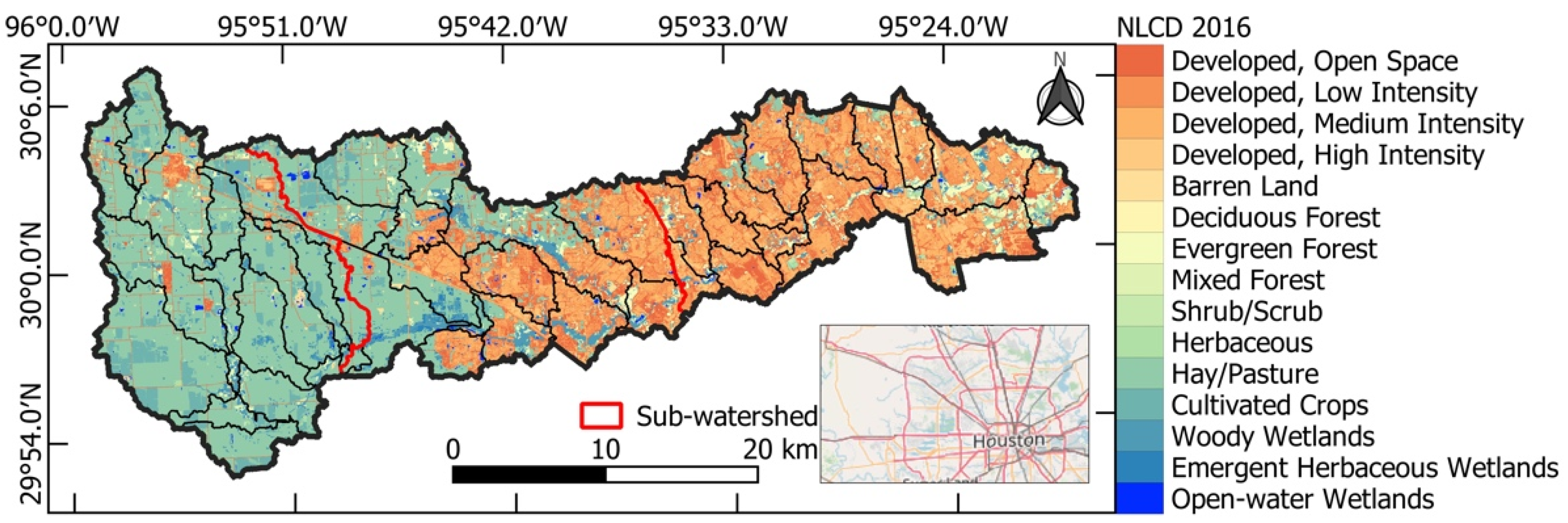
The current study was carried out in the Cypress Creek watershed located in northern Houston, within the Harris County Flood Control District. The first and most significant step for flood mitigation within the study watershed is to successfully identify the locations of the wetlands. Figure 1 shows the geographic location and the land use condition of the study watershed.
As shown in Figure 1, the whole watershed can be delineated into three sub-watersheds [8]. The upstream sub-watershed of the Cypress Creek watershed is mostly natural and agricultural areas, and the midstream sub-watershed is mixing the agricultural area with the residential area. The residential area with estimated 216,000 residents is located within the downstream sub-watershed [31]. The Cypress Creek watershed experiences about two to three flooding events per year on average. For example, it experienced devasting floods during Hurricane Harvey in August 2017. During that event, 82 people died and estimated economic losses were about $180 billion [32]. Therefore, the Cypress Creek watershed is chosen as the study area to delineate the existing open-water wetlands that will be further used for flood mitigation purpose.
2.2. Methods for Existing Wetland Delineation
In order to utilize wetlands for flood mitigation in the study area, it is necessary to understand the spatial distribution and inundation extent of wetlands since this information can be used to estimate their storage capacity [33,34]. However, no single, indisputable, and universally accepted definition of wetlands exists due to the diversity of wetlands in the natural environment and the fact that their dynamic inundation extent changes along the seasons [16]. In order to avoid the dispute on wetland delineation when applying the following indices, we only focused on the wetlands with the open-water features such as lakes, detention and retention ponds, etc. The open-water wetlands are usually open and standing water bodies surrounded by uplands [35]. Various studies [36,37] used remotely-operated siphon system to drain water from wetlands. These wetlands would be ideal for flood mitigation since they may provide sufficient hydraulic head to release water, in turn, increase the storage capacity before a rainfall event, compared with wetlands like swamp or marsh.
2.2.1. Normalized Difference Vegetation Index (NDVI)
The NDVI is a well-established indicator for the presence and condition of vegetation and is also widely used to enhance discrimination between wetland areas and upland features. The use of remote sensing for wetland classification, land cover mapping, and wetland vegetation mapping is shown in different studies [38,39,40,41]. The NDVI is constructed based on the spectral signature differences between the red radiant energy absorbed by the vegetation and the near-infrared energy reflected from the canopy of the vegetation. It is expressed as the normalized ratio of the NIR band and Red band, as shown in Equation (1):
The value of the NDVI ranges from −1.0 to 1.0. For instance, healthy and abundant vegetation reflects strongly in the near-infrared portion of the spectrum while strongly absorbing the visible red light, thus, generating high positive NDVI values. Open-water bodies yield negative values due to red reflectance larger than near-infrared reflectance. Therefore, the NDVI can be applied to delineate open-water wetlands since the lower NDVI values correspond to open water areas in this study.
2.2.2. Normalized Difference Water Index (NDWI)
McFeeters [42] introduced the NDWI to delineate open-water features by combining the Green and NIR bands. It can be written as Equation (2):
where Green is the green band, and NIR is the near-infrared band. All the positive values of the NDWI would be classified as water areas and the negative values as non-water areas.
2.2.3. Topographic Wetness Index (TWI)
The TWI is a conceptually based model that describes the impact of the topography on the water accumulated at a given point and the effect of gravitational force on water movement. It considers the local slope and the upslope drainage area on the topography [22,43]. Since the topography and gravitational force are the driving forces of surface water movement, the wetland location mainly depends on flow path convergence, slope, and the hydraulic conductivity of the soils [44]. Therefore, the TWI also shows the availability of wetland delineation. Developed by Beven et al. [22], the TWI is defined as Equation (3):
where is the local upslope area draining through a certain point per net contour length (equal to the upslope contributing catchment area divided by the contour length along), which is calculated by using a depressionless DEM (the DEM without sinks), and is the local slope (a steepest downslope direction in DEM). The depressionless DEM can be generated in many GIS software by using the “Fill Sink” function. In this study, the Whitebox Geospatial Analysis Tools [24], an open-sources GIS software package, was used to generate the depressionless DEM, and perform other raster calculations. According to its definition, the TWI reflects the tendency of an area to receive water to its tendency to drain water. Therefore, the wetlands tend to locate at the higher value of TWI, where the upslope contributing catchment area is more extensive for collecting an adequate amount of water, and the local slope is smaller for detaining the water.
2.2.4. Deterministic Topographic Wetland Index (DTWI)
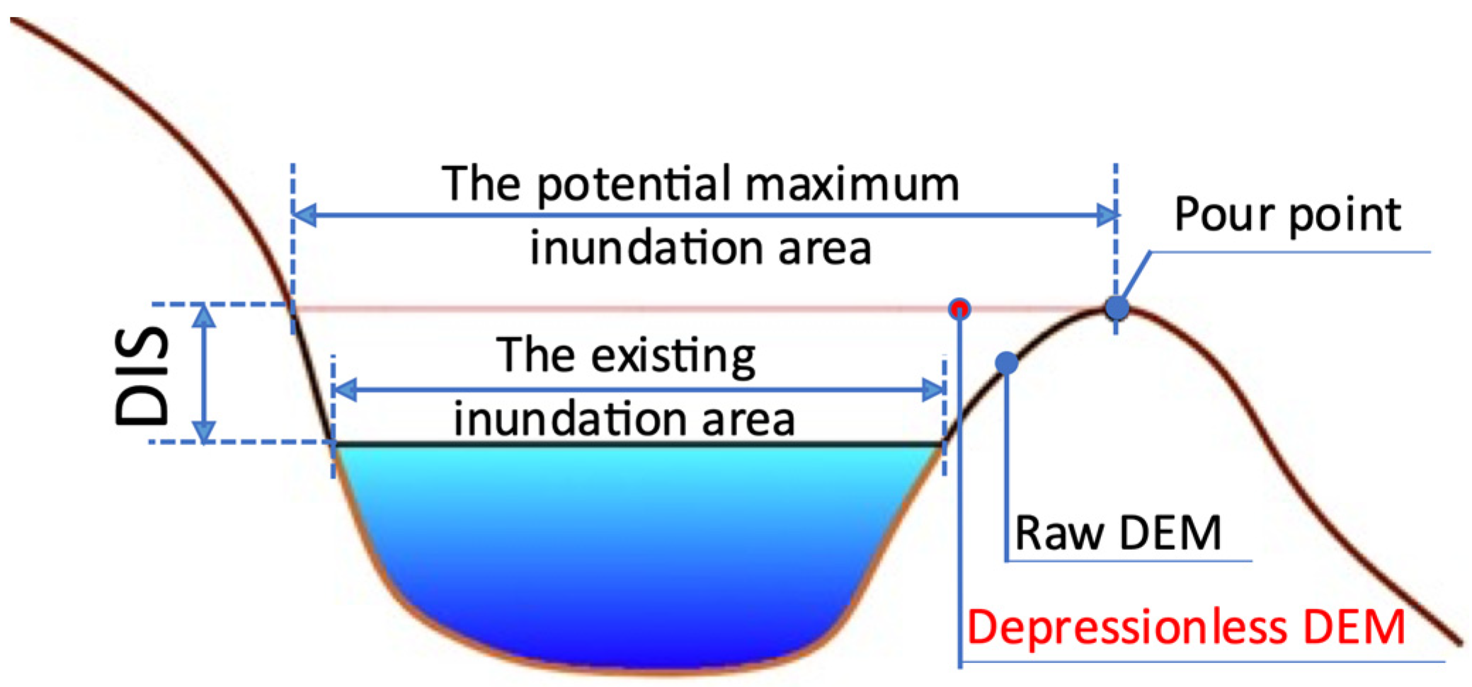
Esri [45] and Wu et al. [24] introduced a fast and straightforward solution to identify the open-water area or the wetland depression by using the “filling-and-spilling” method. The “filling-and-spilling” method is simply subtracting a raw DEM from a depressionless DEM (the DEM without sinks). Sinks are defined as topographic locations that are at a lower elevation than all neighboring cells. The difference between the depressionless DEM and the raw DEM is called Depth in Sink (DIS) in the study of Antoni et al. [46]. This approach can delineate open-water wetlands because the definition of sinks is wholly consistent with the definition of wetland depressions [23]. Therefore, the open-water wetlands are where the pixel value of DIS is bigger than 0. Some studies [47,48,49] also show the application of the “filling-and-spilling” conception for the wetland delineation.
The research conducted by Uuemaa [49] pointed out that DIS bigger than 0 does not always represent wetland areas. It could represent an artificial impoundment formed by the intersections between roadways and streams in the DEM. Additionally, since sinks could also be errors that do not exist on the real terrain, DIS bigger than 0 could be caused by these errors. In order to avoid this mistaken identification of the depression areas, the author’s opinion is that the physical characteristics of water bodies in the DEM should be integrated into the “filling-and-spilling” method.
As depicted in Figure 2, the following three facts can be used to delineation open-water wetlands:
- The water surface in open-water wetlands tends to be in a horizontal plane as water velocity is extremely slow (standing water bodies).
- The local slope of the water surface () is 0 on the LiDAR-derived DEM. This is because LiDAR point clouds show voids in the areas where water bodies occur, and the missing elevation data can be interpolated from a single elevation value obtained from the land edge of the water body.
- The topography should have depression areas that allow water to be detained in the wetlands. Therefore, open-water wetlands should form where the DIS is greater than 0.
Combining these three facts can help to delineate open-water wetland inundation areas rapidly. Therefore, the proposed new deterministic topographic method for wetland delineation is expressed as Equation (4) below,
where is the depth in sink, is the resolution of the DEM, and is the local slope ( in degrees).
To be specific, the wetland can only be located in the ground surface where water can be detained. Therefore, DIS has to be greater than 0 for detaining the water. However, wetlands do not always exist where the DIS is greater than 0 because this could be an abovementioned artificial impoundment. Therefore, a cell in the DEM has to meet two criteria to represent a wetland: a DIS greater than 0 and equal to 0. Obviously, a cell value equal to 1, calculated by the proposed index (DTWI), represents the location of an open-water wetland. Subsequently, a binary imagery will be obtained from the DTWI raster file by exporting cell values equal to 1 into a new raster file with zero background. In the binary imagery, the value of 1 represents the inundation areas of the existing open-water wetlands. In contrast, the value of 0 represents non-water areas. Since it is a logic-based deterministic index, there is no need to perform supervised classification.
2.3. Input Datasets and Data Preprocessing
Table 1 shows the details and purposes of the four spatial datasets which were used in this study. They are National Land Cover Dataset (NLCD), Google satellite imageries, high-resolution bare-earth LiDAR DEM, and four-band color-infrared aerial imagery from the National Agriculture Imagery Program (NAIP).
The high-resolution LiDAR-derived bare-earth DEM was used to calculate the TWI and the DTWI. The cloud-free high-resolution four-band (Red, Green, Blue, and Near-Infrared) aerial imagery from the NAIP was used to calculate the NDWI and the NDVI. Considering that the different resolutions of the datasets could influence the calculation results and the classification accuracy, the LiDAR-derived DEM and the NAIP aerial imagery were resampled into the same resolution (2 m by 2 m) to be consistent with the resolution. In addition, to minimize the topographical changes due to the time span, the LiDAR-derived DEM and the aerial imagery from NAIP used in this study were limited within 2018. In addition, the cloud-free Google satellite imageries from four different years as the main ground truth images were used for the accuracy assessment of the wetland classification.
Since the calculated results of the NDVI, the NDWI, and the TWI are a series of pixel values, the supervised classification is required to classify pixel values into the water areas and the non-water areas for the above-mentioned calculated results. In order to perform supervised classification, the ground-truth training dataset needs to prepare. National Land Cover Dataset (NLCD), containing different earth ground classes, was used to generate the ground truth training sample points rapidly and roughly. Subsequentially, the accuracy of these ground the training sample points were checked and modified if necessarily based on the Google satellite images that were used in this study. Therefore, the resolution of the NLCD (30 m by 30 m) will not influence the accuracy of the supervised classification in this study.
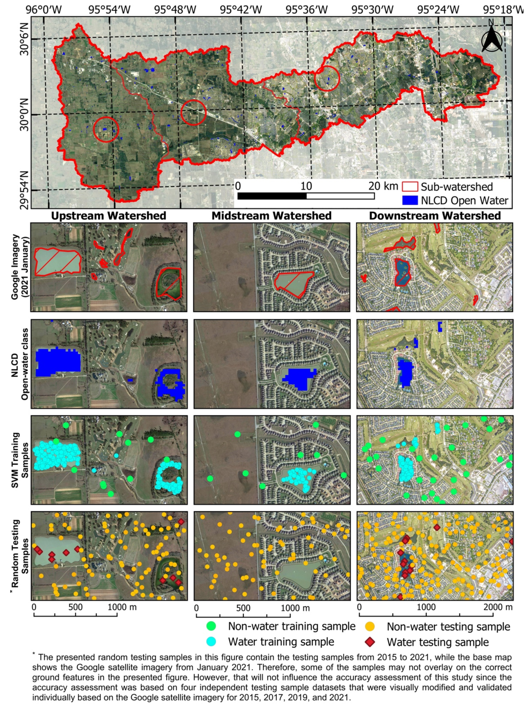
To be specific, first, based on the research objective, the NLCD was only classified into two classes: open-water and non-water areas. The pixel value in the open-water area was set to 1, while the non-water area was set to 0. After that, as shown in Figure 3, the random training sample points (almost 10,000) that would be used for the supervised classification were generated within the open-water areas (4757 training sample points) and the non-water areas (5000 training sample points), separately, by using QGIS. In order to guarantee the accuracy of the ground truth training sample points, the locations of these random training samples were modified manually, based on the high-resolution Google satellite images by careful visual interpretation, if necessary. Subsequently, these training data samples collected the ground-truth information, either the open-water areas (the pixel value equal to 1) or the non-water area (the pixel value equal to 0), from the classified binary NLCD imagery.
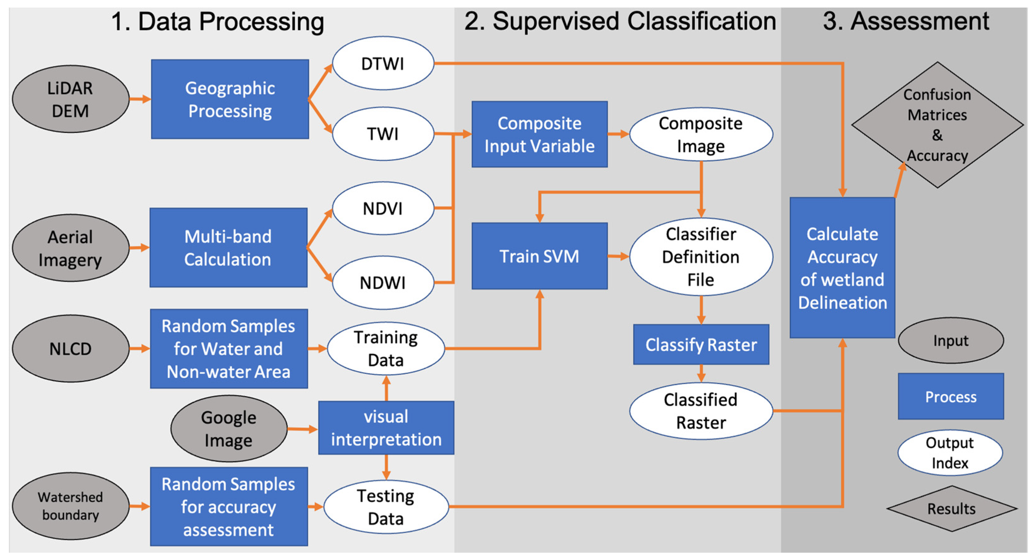
The machine-learning algorithm plays an important role in supervised classification [50]. Support Vector Machine (SVM) is a popular machine-learning algorithm based on the statistical learning theory and the structural risk minimization principle. Since it has a high generalization performance and is suitable for imagery classification with a small training sample set [26], the SVM is chosen for the supervised classification in this study. Except for the DTWI, all the three indices mentioned above used the SVM algorithm to perform supervised classification for wetland area delineation. The supervised classification was performed by QGIS-3.16 Dzetsaka classification tool, a fast and powerful classification plugin for QGIS which has been widely used in other research [51,52,53], and Figure 4 describes the workflow of the data processing for the four indices.
3. Results and Discussion
3.1. The Existing Wetland Delineation
The supervised classification for the chosen indices was successfully performed to classify the pixel value into water and non-water areas by using the SVM algorithm of Dzetsaka classification tool on QGIS. As shown in Table 2, among the SVM training samples, 70% of them were used for machine training, and 30% of them were kept for validation. The TWI shows the minimum classified accuracy and Kappa Coefficient among the chosen indices, which are higher than 90% and 0.8, respectively. The accuracy of the classified results for these three indices is acceptable and the classified imagery of these three indices can be used for further analysis.
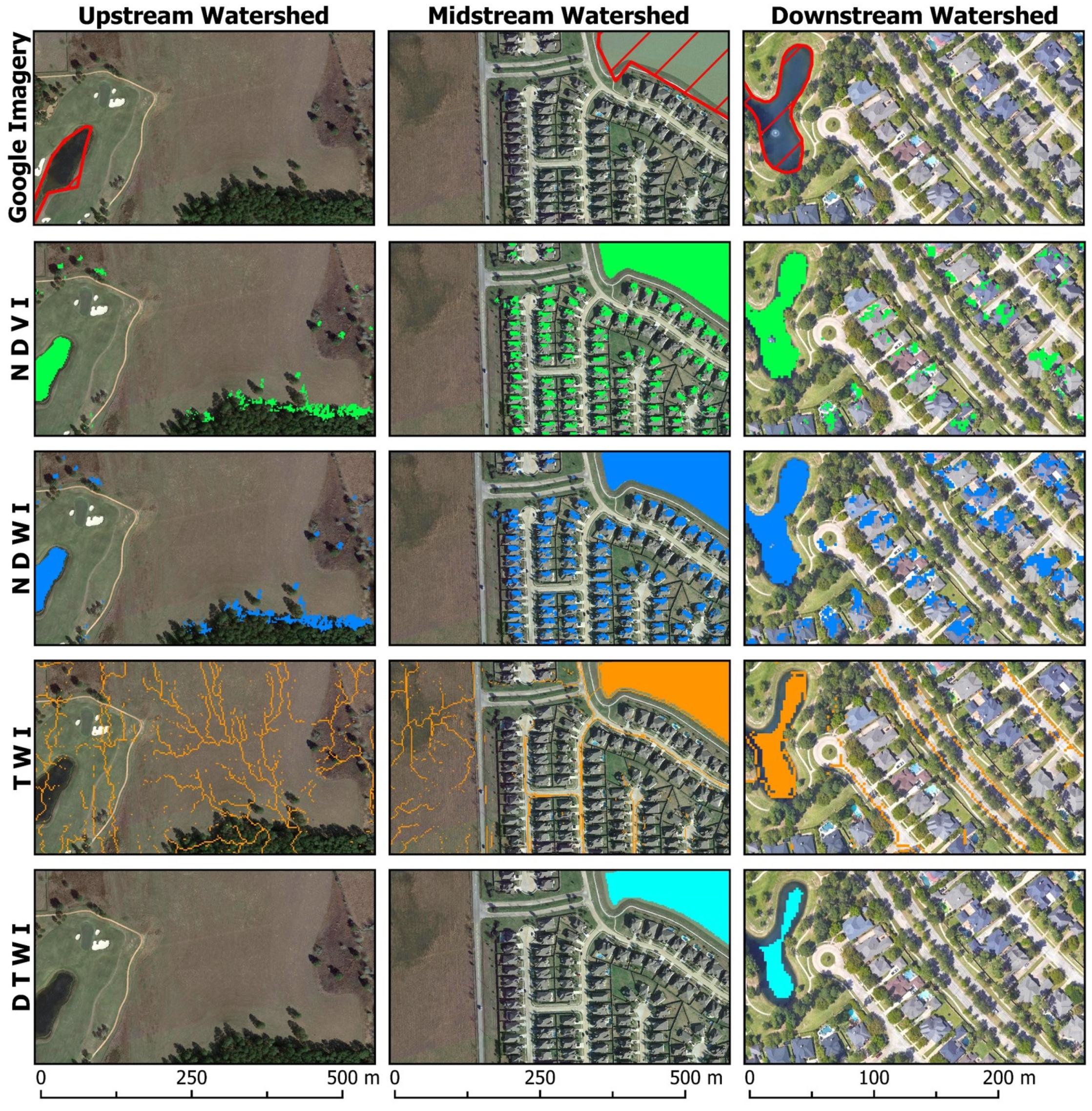
At the same locations presented in Figure 3, Figure 5 below shows the inundation area of the existing open-water wetlands delineated by the four indices mentioned above (NDVI, NDWI, TWI, and DTWI) in the upstream, midstream, and downstream sub-watersheds of the Cypress Creek watershed. According to the results, visually, all four indices can successfully delineate most wetland areas in the natural and residential areas and show similar patterns of waterbody delineation. However, it should be noted that although the NDVI and the NDWI can successfully delineate the wetland areas, they also give a higher response to city infrastructures and shadows, especially the roofs of buildings.
Figure 6 below aims to show the mistakenly classified pixels for the four indices at the same locations presented in Figure 3. Specifically, as shown in Figure 6, the NDVI and the NDWI misclassified the shadows of the trees in the natural/agriculture areas, and the rooftop as well as the shadow of the buildings and partial city infrastructures in residential areas. This is due to the drawback and limitation of the NDVI and the NDWI when using high-resolution optical imagery. Moreover, the TWI also delineates the artificial streams in the natural/agriculture areas, and the roadways in the residential areas. The definition of TWI can explain this phenomenon. The TWI determines possible surface water accumulation zones by quantifying the tendency of a DEM pixel to receive and accumulate water based on the local slope and the upslope contributing area. The upslope contributing area is conventionally calculated by Flow Accumulation function in the GIS platform and a pixel with high Flow Accumulation values also means the pixel has bigger upslope contributing area. Since the artificial streams in agriculture areas and the roadways in the residential areas also have higher flow path convergence (flow accumulation values), which results in higher TWI values, the TWI eventually misclassifies these artificial streams and the roadways as water features. The above-mentioned misclassified pixels from the NDVI, the NDWI, and the TWI can create significant and tedious work for wetland inundation area calculation and storage estimation as they must be removed manually by complex data processes on the GIS platform. However, the above problems can be completely avoided by applying the proposed DTWI.
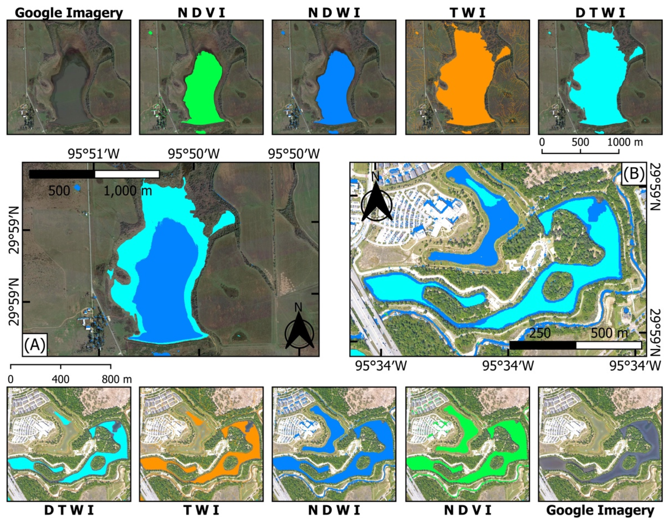
However, there are some differences in the results between the topographic indices (TWI and DTWI) and the optical-imagery indices (NDVI and NDWI). As shown in Figure 7A,B, the wetland inundation areas for these two locations delineated by the DTWI are similar to the TWI. The wetland areas delineated by the NDVI are closed to the NDWI. Nevertheless, the inundation area of the wetland presented in Figure 7A delineated by the two topographic indices is significantly larger than that of the two optical-imagery indices, while the one presented in Figure 7B shows the inundation area delineated by the two topographic indices is obviously smaller than that of the two optical-imagery indices. Since only one optical imagery and one LiDAR-derived bare-ground DEM were applied in this study, the results cannot show the inundation area of a wetland change with time, which is also not the objective of this study. It is well-known that the size and shape of the inundation area of the wetlands vary with time, as water levels fluctuate seasonally.
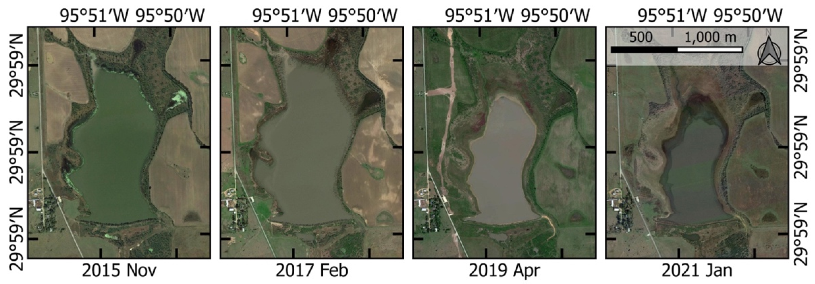
Figure 8 shows the inundation area of the same wetland presented in Figure 7A significantly changes with time. To be specific, the wetland inundation area in the dry season could be significantly smaller than the area in the wet season. One optical image or one DEM can only statically reflect the wetland inundation area at the time of dataset collection. Since the time span exists in the data acquisition between the optical imagery and the LiDAR dataset, as the results show in Figure 7, the inundation area of the existing wetlands delineated by topographic indices can differ from the optical indices in this study.
Furthermore, the inundation area of a wetland is also dependent on the antecedent hydrological condition, the morphological characteristics of the depression wetlands (i.e., the water level-storage-area curve), and the utilization purpose of the wetlands (i.e., irrigation). These factors could cause the inundation area of a wetland to change significantly or even disappear between the time span of the data acquisition. For example, it is worth noting that, in Figure 6, the NDVI and the NDWI delineated the wetland area located at the upstream sub-watershed. In contrast, the TWI and the DTWI did not delineate it as the wetland could have disappeared at the time of the LiDAR data collection.
In conclusion, in order to avoid the impact of the time variation of the wetland inundation area on the accuracy assessment, multiple historical Google satellite images should be applied to comprehensively assess the effectiveness of each index.
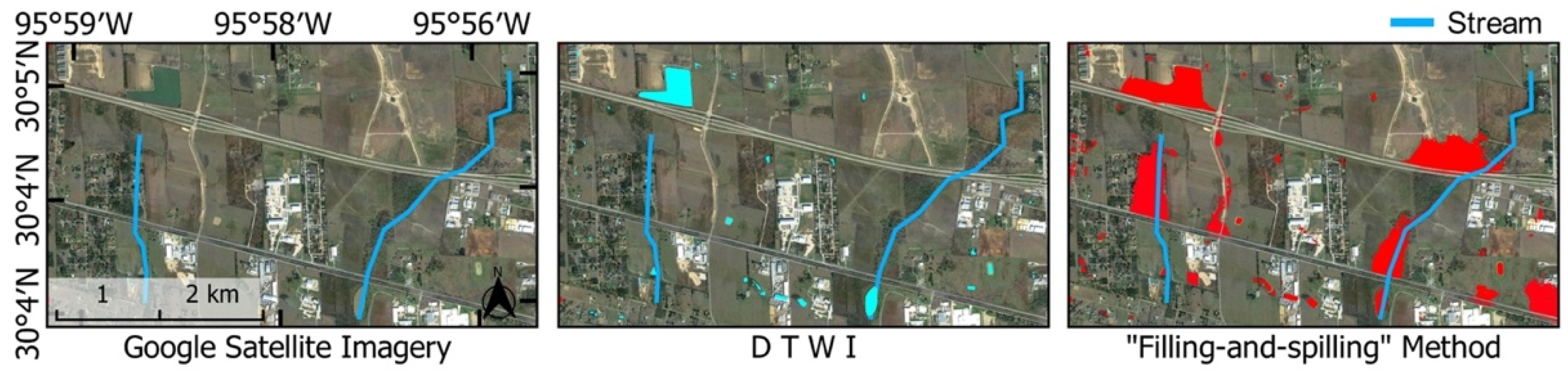
Figure 9 shows the delineated area for the DTWI and the “filling-and-spilling” method. Comparing the difference between these two methods, it can be found that the “filling-and-spilling” method mistakenly delineates the artificial impoundment caused by the intersections between roadways and streams and the DTWI method does not. Therefore, simply using the “fill-and-spilling” method will cause the inundation area to be overestimated in the watershed.
3.2. The Accuracy Assessment
The accuracy assessment of the wetland delineation was quantitatively evaluated by the overall accuracy and the Kappa coefficient calculated from the confusion matrices. The Kappa coefficient equal to 1 represents the perfect agreement with the reference data, while the Kappa coefficient equal to 0 represents complete randomness.
In order to obtain the statistical samples for the confusion matrices and considering that the existence of the time span in the dataset acquisition could impact the accuracy assessment, four independent testing sample datasets, each of them containing 10,000 testing sample points, were generated and validated with the four-year historical Google satellite imageries, individually. The function of “Random Point in Polygon” in the QGIS was used to generate 10,000 testing sample points located randomly within the Cypress Creek watershed. As the study area cannot be visited, these 10,000 random testing sample points were assigned a ground truth value (1 represents the water areas and 0 represents the non-water areas) based on their locations on the Google satellite imagery by visually interpreted carefully. In such a way, the 10,000 ground truth values were stored in the first column of the attribute table of the random testing data sample points. These ground truth values were used as the actual class for the confusion matrices. Subsequently, these testing sample points extracted the pixel values from the classified raster files of the NDVI, the NDWI, and the TWI, and the calculated raster file of the DTWI sequentially. These pixel values were stored in the second, third, fourth, and fifth columns of the attribute table, respectively. They were used as the predicted class for the confusion matrices.
The confusion matrices were calculated to summarize the testing points of wetland agreement (T.P.), non-wetland agreement (T.N.), false-negative predictions (F.N.) (cases where true wetland testing points were predicted to be non-wetland), and false-positive predictions (F.P.) (case where true non-wetland testing points were predicated to be wetland).
The overall accuracy and the Kappa coefficient are calculated by Equations (5) and (6), and the confusion matrices for four indices from selected four-year Google satellite images is shown in Table 3.
As shown in Table 3, although the different historical Google satellite imagery has an impact on the accuracy assessment, such impact can be neglected since the difference of the overall accuracy for each index is less than 1% within four different historical Google satellite images. Therefore, the existence of the time span in the dataset acquisition will not substantially influence the accuracy assessment in this study.
By summarizing the four independent testing sample datasets, the DTWI provides the best overall accuracy among the four indices in cross-validation (98.90%), and the Kappa coefficient of the DTWI shows substantial agreement [54]. The lowest value of overall accuracy and the Kappa coefficient is the TWI, which is only 93.79% and 0.245, respectively. Such a lower Kappa coefficient of the TWI raised the research team’s concerns about whether the mistakes existed during the research calculation. After double-checking the calculation procedures, the whole team confirmed that there were no calculation mistakes, and the TWI should provide a lower Kappa coefficient. As shown in Figure 6, the TWI mistakenly classifies the artificial streams and roadways into the water features within the whole watershed, resulting in the cases where true non-wetland testing points were predicated to be wetland (F.P.) being significantly higher. According to the result shown in Table 3, the TWI shows the highest case of F.P. among these four indices, which is 2270. Such the highest value of the F.P. case decreases the Kappa coefficient and the overall accuracy of the TWI. The difference in the overall accuracy between the NDVI and NDWI is less than 1%, and the Kappa coefficient of both shows moderate agreement.
Although in comparing the DTWI and the NDVI for the 4-year overall accuracy assessment there is only a 1% improvement of the overall accuracy, which is not significant, the DTWI is a simple and rapid solution which does not require supervised classification. It is worth mentioning that the similarity of the overall accuracy between the DTWI and the NDVI further indicates that the DTWI can replace the NDVI, the NDWI, and the TWI for the open-water wetland delineation in the study area.
4. Conclusions
Identification and delineation of wetlands provide critical information for various purposes, including flood mitigation. The increasing availability of fine-resolution DEMs data and the high-resolution optical images makes it possible to obtain detailed information about topographic surface features, including wetlands. However, conventional methods for wetland delineation need to perform supervised classification to guarantee a desirable classification accuracy. This paper presents an efficient and accurate method for delineating open-water wetlands without performing supervised classification. The proposed DTWI delineates the wetlands by considering the physical characteristics of a wetland on the ground surface.
Considering the time variation of the inundation area of the wetlands could influence the accuracy assessment of the four indices in this study, four-year historical cloud-free Google satellite images were chosen as the ground truth reference datasets. The results show that although the different historical Google satellite imagery has an impact on the accuracy assessment, such impact can be ignored considering the results change within 1% for the four indices.
Two optical imagery approaches (the NDVI and the NDWI) show an acceptable and satisfying accuracy (97.80% and 96.88%, respectively) on the wetland delineation. However, the city infrastructure, such as roof shadows, are widely mistakenly delineated as water features within the study area. Moreover, TWI misclassifies the artificial stream and the roadways into the water features, resulting in the lowest accuracy assessment. Without removing these mistakenly delineated areas manually by complex data processing on the GIS platform, the inundation area of the watershed will be overestimated, resulting in an inaccurate estimation of the water storage capacity.
Although the DTWI shows the highest accuracy assessment, comparing the NDVI with the DTWI, the improvement of the accuracy assessment, which is only 1.1%, is not significant. However, such insignificant improvement indicates the DTWI can replace the classic method to delineate wetland inundation areas. Moreover, unlike the optical imagery approach, it does not generate any other irrelevant results, resulting in the highest accuracy of applying the DTWI to delineate wetlands.
Overall, compared to the other methods investigated, the DTWI method was found to minimize mistaken wetlands with infrastructure, shadows, streams, and artificial impoundment and showed the highest accuracy assessment.
The results for the study area show that the proposed deterministic topographic method can delineate wetland areas more accurately and efficiently than the classic methods compared in this study, namely the NDVI, the NDWI, and the TWI. It has great potential for being applied to the large-scale watershed flood mitigation analysis. The finding of this study provides an alternative to delineate wetlands by using LiDAR-derived DEM only.
Author Contributions
Major conceptualization and methodology, L.B.; providing the guidance for the formal analysis, A.M.M. and A.S.L.; validation of the final results, V.V. and Z.Y. All authors have read and agreed to the published version of the manuscript.
Funding
The first and third authors of this research were funded by the National Science Foundation through NSF/ENG/CBET grant number 1805417 and through NSF/DBI/BIO grant number 1820778.
Conflicts of Interest
The authors declare no conflict of interest.
References
- Lewis, J.; William, M. Wetlands Explained: Wetland Science, Policy, and Politics in America; Oxford University Press: Oxford, UK, 2001. [Google Scholar]
- Bullock, A.; Acreman, M. The role of wetlands in the hydrological cycle. Hydrol. Earth Syst. Sci. 2003, 7, 358–389. [Google Scholar] [CrossRef] [Green Version]
- Fausold, C.J.; Lilieholm, R.J. The Economic Value of Open Space: A Review and Synthesis. Environ. Manag. 1999, 23, 307–320. [Google Scholar] [CrossRef]
- Godschalk, D.; Beatley, T.; Berke, P.; Brower, D.; Kaiser, E.J. Natural Hazard Mitigation: Recasting Disaster Policy and Planning; Island Press: Washington, DC, USA, 1998. [Google Scholar]
- Nivitzki, R. Effects of Lakes and Wetlands on Floodflows and Base Flows in Selected Northern and Eastern States. In Proceedings of the Conference Wetlands of the Chesapeake, Easton, MD, USA, 9–11 April 1985; pp. 143–154. [Google Scholar]
- Leon, A.S.; Tang, Y.; Qin, L.; Chen, D. A MATLAB framework for forecasting optimal flow releases in a multi-storage system for flood control. Environ. Model. Softw. 2020, 125, 104618. [Google Scholar] [CrossRef]
- Tang, Y.; Leon, A.S.; Kavvas, M.L. Impact of Size and Location of Wetlands on Watershed-Scale Flood Control. Water Resour. Manag. 2020, 34, 1693–1707. [Google Scholar] [CrossRef]
- Tang, Y.; Leon, A.S.; Kavvas, M.L. Impact of Dynamic Storage Management of Wetlands and Shallow Ponds on Watershed-scale Flood Control. Water Resour. Manag. 2020, 34, 1305–1318. [Google Scholar] [CrossRef]
- Sørensen, R.; Zinko, U.; Seibert, J. On the calculation of the topographic wetness index: Evaluation of different methods based on field observations. Hydrol. Earth Syst. Sci. 2006, 10, 101–112. [Google Scholar] [CrossRef] [Green Version]
- McKergow, L.A.; Gallant, J.C.; Dowling, T.I. Modelling Wetland Extent Using Terrain Indices, Lake Taupo, NZ. In Proceedings of the MODSIM07—Land, Water and Environmental Management: Integrated Systems for Sustainability, Proceedings, Christchurch, New Zealand, 10–13 December 2007; pp. 1335–1341. [Google Scholar]
- O’Neil, G.L.; Goodall, J.; Watson, L.T. Evaluating the potential for site-specific modification of LiDAR DEM derivatives to improve environmental planning-scale wetland identification using Random Forest classification. J. Hydrol. 2018, 559, 192–208. [Google Scholar] [CrossRef]
- Lidzhegu, Z.; Ellery, W.; Mantel, S.; Hughes, D. Delineating wetland areas from the cut-and-fill method using a Digital Elevation Model (DEM). S. Afr. Geogr. J. 2020, 102, 97–115. [Google Scholar] [CrossRef]
- Melesse, A.M.; Weng, Q.; Thenkabail, P.S.; Senay, G.B. Remote Sensing Sensors and Applications in Environmental Resources Mapping and Modelling. Sensors 2007, 7, 3209–3241. [Google Scholar] [CrossRef] [PubMed] [Green Version]
- Zhou, Y.; Dong, J.; Xiao, X.; Xiao, T.; Yang, Z.; Zhao, G.; Zou, Z.; Qin, Y. Open Surface Water Mapping Algorithms: A Comparison of Water-Related Spectral Indices and Sensors. Water 2017, 9, 256. [Google Scholar] [CrossRef]
- Mahdianpari, M.; Granger, J.E.; Mohammadimanesh, F.; Salehi, B.; Brisco, B.; Homayouni, S.; Gill, E.; Huberty, B.; Lang, M. Meta-Analysis of Wetland Classification Using Remote Sensing: A Systematic Review of a 40-Year Trend in North America. Remote Sens. 2020, 12, 1882. [Google Scholar] [CrossRef]
- Wu, Q. GIS and Remote Sensing Applications in Wetland Mapping and Monitoring. Compr. Geogr. Inf. Syst. 2018, 3, 140–157. [Google Scholar] [CrossRef]
- Worstell, B.B.; Poppenga, S.K.; Evans, G.A.; Prince, S. Lidar Point Density Analysis: Implications for Identifying Water Bodies; US Geological Survey: Reston, VA, USA, 2014.
- Toscano, G.; Acharjee, P.; McCormick, C.; Devarajan, V. Water Surface Elevation Calculation Using LiDAR Data. In Proceedings of the ASPRS Conference, Tampa, FL, USA, 4–8 May 2015. [Google Scholar]
- Bochow, M.; Heim, B.; Küster, T.; Rogaß, C.; Bartsch, I.; Segl, K.; Reigber, S.; Kaufmann, H. On the use of airborne imaging spectroscopy data for the automatic detection and delineation of surface water bodies. In Remote Sensing of Planet Earth; InTech: London, UK, 2012; pp. 1–22. [Google Scholar]
- Jahncke, R.; Leblon, B.; Bush, P.; LaRocque, A. Mapping wetlands in Nova Scotia with multi-beam RADARSAT-2 Polarimetric SAR, optical satellite imagery, and Lidar data. Int. J. Appl. Earth Obs. Geoinf. 2018, 68, 139–156. [Google Scholar] [CrossRef]
- Ozesmi, S.L.; Bauer, M.E. Satellite remote sensing of wetlands. Wetl. Ecol. Manag. 2002, 10, 381–402. [Google Scholar] [CrossRef]
- Beven, K.J.; Kirkby, M.J. A physically based, variable contributing area model of basin hydrology/Un modèle à base physique de zone d’appel variable de l’hydrologie du bassin versant. Hydrol. Sci. J. 1979, 24, 43–69. [Google Scholar] [CrossRef] [Green Version]
- Jenkins, D.G.; McCauley, L.A. GIS, SINKS, FILL, and Disappearing Wetlands: Unintended Consequences in Algorithm Development and Use. In Proceedings of the 2006 ACM Symposium on Applied Computing, Dijon, France, 23–27 April 2006; Association for Computing Machinery: New York, NY, USA, 2006; pp. 277–282. [Google Scholar]
- Wu, Q.; Lane, C.R.; Wang, L.; Vanderhoof, M.; Christensen, J.R.; Liu, H. Efficient Delineation of Nested Depression Hierarchy in Digital Elevation Models for Hydrological Analysis Using Level-Set Method. JAWRA J. Am. Water Resour. Assoc. 2019, 55, 354–368. [Google Scholar] [CrossRef]
- Chapelle, O.; Haffner, P.; Vapnik, V.N. Support vector machines for histogram-based image classification. IEEE Trans. Neural Netw. 1999, 10, 1055–1064. [Google Scholar] [CrossRef]
- Melgani, F.; Bruzzone, L. Classification of hyperspectral remote sensing images with support vector machines. IEEE Trans. Geosci. Remote Sens. 2004, 42, 1778–1790. [Google Scholar] [CrossRef] [Green Version]
- Breiman, L. Bagging Predictors. Mach. Learn. 1996, 24, 123–140. [Google Scholar] [CrossRef] [Green Version]
- Rokach, L.; Maimon, O. Top-Down Induction of Decision Trees Classifiers—A Survey. IEEE Trans. Syst. Man, Cybern. Part C Appl. Rev. 2005, 35, 476–487. [Google Scholar] [CrossRef] [Green Version]
- Ho, T.K. The random subspace method for constructing decision forests. IEEE Trans. Pattern Anal. Mach. Intell. 1998, 20, 832–844. [Google Scholar] [CrossRef] [Green Version]
- Thapa, A.; Bradford, L.; Strickert, G.; Yu, X.; Johnston, A.; Watson-Daniels, K. “Garbage in, Garbage Out” Does Not Hold True for Indigenous Community Flood Extent Modeling in the Prairie Pothole Region. Water 2019, 11, 2486. [Google Scholar] [CrossRef] [Green Version]
- Teague, A. Development of a Distributed Water Quality Model Using Advanced Hydrologic Simulation. Ph.D. Thesis, Rice University, Houston, TX, USA, August 2011. [Google Scholar]
- Leon, A.S.; Verma, V. Towards Smart and Green Flood Control: Remote and Optimal Operation of Control Structures in a Network of Storage Systems for Mitigating Floods. In Proceedings of the World Environmental and Water Resources Congress 2019, Pittsburgh, PA, USA, 19–23 May 2019; pp. 177–189. [Google Scholar]
- Wu, Q.; Lane, C.R. Delineation and Quantification of Wetland Depressions in the Prairie Pothole Region of North Dakota. Wetlands 2016, 36, 215–227. [Google Scholar] [CrossRef]
- Gleason, R.A.; Tangen, B.A.; Laubhan, M.K.; Kermes, K.E.; Euliss, N.H., Jr. Estimating Water Storage Capacity of Existing and Potentially Restorable Wetland Depressions in a Subbasin of the Red River of the North; USGS Northern Prairie Wildlife Research Center: Jamestown, ND, USA, 2007; p. 89.
- Golden, H.E.; Lane, C.; Amatya, D.M.; Bandilla, K.W.; Kiperwas, H.R.; Knightes, C.D.; Ssegane, H. Hydrologic connectivity between geographically isolated wetlands and surface water systems: A review of select modeling methods. Environ. Model. Softw. 2014, 53, 190–206. [Google Scholar] [CrossRef]
- Verma, V.; Bian, L.; Rojali, A.; Ozecik, D.; Leon, A. A Remotely Controlled Framework for Gravity-Driven Water Release in Shallow and Not Shallow Storage Ponds. In Proceedings of the World Environmental and Water Resources Congress 2020, Henderson, NV, USA, 17–21 May 2020; American Society of Civil Engineers (ASCE): Reston, VG, USA, 2020; pp. 12–22. [Google Scholar]
- Qin, L.; Leon, A.S.; Bian, L.-L.; Dong, L.-L.; Verma, V.; Yolcu, A. A Remotely-Operated Siphon System for Water Release from Wetlands and Shallow Ponds. IEEE Access 2019, 7, 157680–157687. [Google Scholar] [CrossRef]
- Narumalani, S.; Jensen, J.R.; Burkhalter, S.; Althausen, J.D.; Mackey, H.E., Jr. Aquatic Macrophyte Modeling Using GIS and Logistic Multiple Regression. Photogramm. Eng. Remote Sens. 1997, 63, 41–49. [Google Scholar]
- Melesse, A.M.; Jordan, J.D.; Graham, W.D. Enhancing Land Cover Mapping using Landsat Derived Surface Temperature and NDVI. In Proceedings of the World Water and Environmental Resources, Orlando, FL, USA, 20–24 May 2001; pp. 1–7. [Google Scholar]
- Hui, Y.; Rongqun, Z.; Xianwen, L. Classification of Wetland from TM Imageries Based on Decision Tree. WSEAS Trans. Inf. Sci. Appl. 2009, 6, 1155–1164. [Google Scholar]
- Lane, C.R.; Liu, H.; Autrey, B.C.; Anenkhonov, O.A.; Chepinoga, V.V.; Wu, Q. Improved Wetland Classification Using Eight-Band High Resolution Satellite Imagery and a Hybrid Approach. Remote Sens. 2014, 6, 12187–12216. [Google Scholar] [CrossRef] [Green Version]
- McFeeters, S.K. The use of the Normalized Difference Water Index (NDWI) in the delineation of open water features. Int. J. Remote Sens. 1996, 17, 1425–1432. [Google Scholar] [CrossRef]
- Beven, K. Runoff Production and Flood Frequency in Catchments of Order n: An Alternative Approach. In Climate Change Impacts on Water Resources; Springer Science and Business Media LLC: Berlin/Heidelberg, Germany, 1986; pp. 107–131. [Google Scholar]
- Infascelli, R.; Faugno, S.; Pindozzi, S.; Boccia, L.; Merot, P. Testing Different Topographic Indexes to Predict Wetlands Distribution. Procedia Environ. Sci. 2013, 19, 733–746. [Google Scholar] [CrossRef] [Green Version]
- Esri Find Areas at Risk of Flooding in a Cloudburst: Use ModelBuilder to Analyze Drainage Problems When Extreme Rainfall Hits Denmark. Available online: https://learn.arcgis.com/en/projects/find-areas-at-risk-of-flooding-in-a-cloudburst/ (accessed on 30 December 2020).
- Antonić, O.; Hatic, D.; Pernar, R. DEM-based depth in sink as an environmental estimator. Ecol. Model. 2001, 138, 247–254. [Google Scholar] [CrossRef]
- Wu, Q.; Lane, C.R.; Li, X.; Zhao, K.; Zhou, Y.; Clinton, N.; DeVries, B.; Golden, H.; Lang, M.W. Integrating LiDAR data and multi-temporal aerial imagery to map wetland inundation dynamics using Google Earth Engine. Remote Sens. Environ. 2019, 228, 1–13. [Google Scholar] [CrossRef] [PubMed] [Green Version]
- Wang, L.; Liu, H. An efficient method for identifying and filling surface depressions in digital elevation models for hydrologic analysis and modelling. Int. J. Geogr. Inf. Sci. 2006, 20, 193–213. [Google Scholar] [CrossRef]
- Uuemaa, E.; Hughes, A.O.; Tanner, C.C. Identifying Feasible Locations for Wetland Creation or Restoration in Catchments by Suitability Modelling Using Light Detection and Ranging (LiDAR) Digital Elevation Model (DEM). Water 2018, 10, 464. [Google Scholar] [CrossRef] [Green Version]
- Huang, X.; Xie, C.; Fang, X.; Zhang, L. Combining Pixel- and Object-Based Machine Learning for Identification of Water-Body Types From Urban High-Resolution Remote-Sensing Imagery. IEEE J. Sel. Top. Appl. Earth Obs. Remote Sens. 2015, 8, 2097–2110. [Google Scholar] [CrossRef]
- Karasiak, N. Dzetsaka Qgis Classification Plugin 2016. Available online: https://github.com/nkarasiak/dzetsaka (accessed on 9 September 2021).
- Karasiak, N.; Perbet, P. Remote Sensing of Distinctive Vegetation in Guiana Amazonian Park. QGIS Appl. Agric. For. 2018, 2, 215–245. [Google Scholar] [CrossRef]
- Sejati, A.W.; Buchori, I.; Kurniawati, S.; Brana, Y.C.; Fariha, T.I. Quantifying the impact of industrialization on blue carbon storage in the coastal area of Metropolitan Semarang, Indonesia. Appl. Geogr. 2020, 124, 102319. [Google Scholar] [CrossRef]
- Cohen’s Kappa. Available online: https://en.wikipedia.org/wiki/Cohen%27s_kappa (accessed on 9 September 2021).
Figure 1.
The geographic location of the study watershed.

Figure 2.
The conceptual figure for the presentation of the characteristics of the open-water wetland on the DEM.
Figure 2.
The conceptual figure for the presentation of the characteristics of the open-water wetland on the DEM.

Figure 3.
The ground truth sample points used for the supervised classification and the accuracy assessment within the Cypress Creek watershed.
Figure 3.
The ground truth sample points used for the supervised classification and the accuracy assessment within the Cypress Creek watershed.

Figure 4.
The workflow of data processing of the indices mentioned above.

Figure 5.
The wetland delineation of four indices in upstream (natural/agricultural), midstream (mixed agriculture-residential), and downstream (residential) sub-watersheds.
Figure 5.
The wetland delineation of four indices in upstream (natural/agricultural), midstream (mixed agriculture-residential), and downstream (residential) sub-watersheds.

Figure 6.
The mistakenly classified pixels of the four indices in the upstream (natural/agricultural area), the midstream (mixed agriculture-residential area), and the downstream (residential area) watersheds.
Figure 6.
The mistakenly classified pixels of the four indices in the upstream (natural/agricultural area), the midstream (mixed agriculture-residential area), and the downstream (residential area) watersheds.

Figure 7.
The comparison for the two typical cases of delineation area of the four indices (A) the area delineated by the optical imagery approach is bigger than the topographic approach (B) the area delineated by the optical imagery approach is smaller than the topographic approach.
Figure 7.
The comparison for the two typical cases of delineation area of the four indices (A) the area delineated by the optical imagery approach is bigger than the topographic approach (B) the area delineated by the optical imagery approach is smaller than the topographic approach.

Figure 8.
Time variation of wetland inundation area.

Figure 9.
Delineated area for the DTWI and the “filling-and-spilling” method.


Table 1.
The information of datasets and their usage for the study.
| Dataset | Band | Original Resolution | Resample Resolution | Acquisition Date | Custodian | Use in the Study |
|---|---|---|---|---|---|---|
| NLCD | 30 m | 30 m | 2016 | United States Geological Survey | To generate the training samples rapidly and roughly. Before the training samples used for supervised classification, their accuracy will be modified by Google satellite images, if necessary. | |
| NAIP | B: 435–496 nm | 0.6 m | 2 m | 2018 December | To calculate NDWI and NDVI for wetland delineation. | |
| G: 525–585 nm | ||||||
| R: 619–651 nm | ||||||
| NIR: 808–882 nm | ||||||
| LiDAR derived DEM | 1.5 m | 2 m | 2018 October | Texas Natural Resources Information System | To calculate TWI and DTWI. | |
| Google Satellite Imagery | N.A. | N.A. | 2015 November | Google Earth | As primary ground truth data reference for visual interpretation of the generated testing samples and the comparison of the calculated results. | |
| 2017 February | ||||||
| 2019 April | ||||||
| 2021 January |
Table 2.
The index classification results by using the SVM algorithm of Dzetsaka classification tool.
Table 2.
The index classification results by using the SVM algorithm of Dzetsaka classification tool.
| Index | Training Algorithm | Training | Validation | Kappa | Classified Accuracy |
|---|---|---|---|---|---|
| NDVI | SVM | 70% | 30% | 0.955 | 97.74% |
| NDWI | 0.943 | 97.17% | |||
| TWI | 0.811 | 90.57% |
Table 3.
The confusion matrices and the accuracy assessment.
| Predict Class | Positive | Negative | Accuracy Assessment | |||
|---|---|---|---|---|---|---|
| Actual Class | Positive | Negative | Positive | Negative | Kappa Coefficient | Overall Accuracy |
| Output Case | T.P. | F.P. | F.N. | T.N. | ||
| Normalized Difference Vegetation Index | ||||||
| November 2015 | 120 | 170 | 30 | 9680 | 0.536 | 98.00% |
| February 2017 | 106 | 187 | 51 | 9656 | 0.460 | 97.62% |
| April 2019 | 106 | 155 | 45 | 9694 | 0.505 | 98.00% |
| January 2021 | 133 | 172 | 72 | 9623 | 0.510 | 97.56% |
| Normalized Difference Water Index | ||||||
| November 2015 | 121 | 268 | 29 | 9582 | 0.437 | 97.03% |
| February 2017 | 106 | 286 | 51 | 9557 | 0.372 | 96.63% |
| April 2019 | 108 | 239 | 43 | 9610 | 0.432 | 97.18% |
| January 2021 | 130 | 258 | 75 | 9537 | 0.423 | 96.69% |
| Topographic Wetness Index | ||||||
| November 2015 | 115 | 542 | 35 | 9308 | 0.267 | 94.23% |
| February 2017 | 109 | 591 | 48 | 9252 | 0.235 | 93.61% |
| April 2019 | 95 | 595 | 56 | 9254 | 0.206 | 93.49% |
| January 2021 | 129 | 542 | 76 | 9253 | 0.272 | 93.82% |
| Deterministic Topographic Wetland Index | ||||||
| November 2015 | 105 | 39 | 45 | 9811 | 0.710 | 99.16% |
| February 2017 | 99 | 49 | 58 | 9794 | 0.644 | 98.93% |
| April 2019 | 85 | 54 | 66 | 9795 | 0.580 | 98.80% |
| January 2021 | 114 | 38 | 91 | 9757 | 0.632 | 98.71% |
| Overall Accuracy Assessment for 4-year ground truth samples | ||||||
| NDVI | 465 | 684 | 198 | 38,653 | 0.503 | 97.80% |
| NDWI | 465 | 1051 | 198 | 38,286 | 0.413 | 96.88% |
| TWI | 448 | 2270 | 215 | 37,067 | 0.245 | 93.79% |
| DTWI | 403 | 180 | 260 | 39,157 | 0.641 | 98.90% |
Publisher’s Note: MDPI stays neutral with regard to jurisdictional claims in published maps and institutional affiliations. |
© 2021 by the authors. Licensee MDPI, Basel, Switzerland. This article is an open access article distributed under the terms and conditions of the Creative Commons Attribution (CC BY) license (https://creativecommons.org/licenses/by/4.0/).
Share and Cite
MDPI and ACS Style
Bian, L.; Melesse, A.M.; Leon, A.S.; Verma, V.; Yin, Z. A Deterministic Topographic Wetland Index Based on LiDAR-Derived DEM for Delineating Open-Water Wetlands. Water 2021, 13, 2487. https://doi.org/10.3390/w13182487
AMA Style
Bian L, Melesse AM, Leon AS, Verma V, Yin Z. A Deterministic Topographic Wetland Index Based on LiDAR-Derived DEM for Delineating Open-Water Wetlands. Water. 2021; 13(18):2487. https://doi.org/10.3390/w13182487
Chicago/Turabian StyleBian, Linlong, Assefa M. Melesse, Arturo S. Leon, Vivek Verma, and Zeda Yin. 2021. "A Deterministic Topographic Wetland Index Based on LiDAR-Derived DEM for Delineating Open-Water Wetlands" Water 13, no. 18: 2487. https://doi.org/10.3390/w13182487
Note that from the first issue of 2016, this journal uses article numbers instead of page numbers. See further details here.