What’s on the Menu for the Resident Brown Trout in a Rich Limestone Stream?

Abstract

Examination of brown trout seasonal diet variation and investigation of terrestrial prey importance in a food-rich stream using four indices of prey importance (number and weight abundance, frequency of occurrence, index of relative importance) revealed that aquatic prey constituted the major part of the diet (>90%) throughout the examined period. Despite Gammaridae being the most abundant in the environment, other less abundant organisms appeared to be important prey, including terrestrial organisms, with maximum consumption in September. The electivity index showed a positive selection of rare prey types; Tokeshi’s model revealed a specialist strategy for most of the population, except for those of 1+ age, who were inclining to generalist strategy. Diet diversity increased throughout April to October, and ages 1+ and 2+ exhibited a more diverse diet than older ages. Diet overlap between age classes was considerable, with less overlap observed in the later season. This pattern of differentiation in the diet of brown trout age classes and their feeding plasticity over seasonal scales, as observed in this food-rich stream, provides a starting point for further examination of this topic in streams with similar or different food richness and availability.

1. Introduction

The socioeconomic importance of brown trout (Salmo trutta L., 1758) as an attractive fish species in recreational fishing puts this species in the spotlight of numerous ecological studies [1,2,3,4,5,6,7,8,9,10,11]. Aside from a few basic requirements it shares with other salmonids, brown trout has a worldwide distribution and can live in habitats that may differ significantly, thus making each local study a valuable contribution to knowledge about the feeding patterns and ecological plasticity of this species.

Favorable water temperature and physicochemical characteristics, stable water level, habitat heterogeneity, and sufficient food supply support salmonid growth [12]. Concerning its food requirements, brown trout is a carnivore that feeds on aquatic and terrestrial macroinvertebrates and smaller fish. As a visual forager, it relies on its good vision and agility to catch prey from the stream bed, drift, and water surface, and even airborne prey [13]. Life in a stream or a small river is challenging, with the fish foraging while constantly struggling with water flow and the fluctuating quantity and quality of available food. For these reasons, stream-dwelling brown trout has slower growth rates [14] in comparison with migratory, sea, or lake trout, which inhabit the more resilient ecosystems of oceans and lakes. In some rivers, the food available to brown trout can be diverse and abundant; in others, it can be diverse but not as abundant. Some rivers can be depleted of life so that brown trout struggles to survive and its growth is impeded. As fry, brown trout mainly feed on small benthic invertebrates.

As they grow, they feed on larger invertebrate prey (aquatic, aerial, terrestrial) and finally fish [15]. Piscivory usually begins when 20–30 cm of body length is reached [16,17]. This ontogenetic shift in diet follows morphological changes during growth, primarily increased mouth-gape size and strength for swimming and chasing prey [2,18]. The energy spent on catching prey of any size is similar, yet a bigger prey yields more energy, so salmonids will grow larger where a larger prey is available [14,19].

Although older fish feed on larger invertebrate and fish prey and rely more on terrestrial prey, they do not disregard smaller prey [8]. Several studies have shown that the biggest differences are between early periods of life (larvae and juveniles), whereas after the age of 2+ (i.e., adulthood), dietary differences are minimal [18,20]. Nevertheless, some differences between adult males and females have been reported, especially during the reproductive period, caused mainly by male territoriality [10]. Intraspecific hierarchies can result in dominant fish maintaining optimal positions for feeding, with optimal access to food resources, thereby achieving the highest specific growth rates [21]. Competition for food between age classes is compensated by different microhabitat preferences, strategies, and preying on different prey [3].

Salmonids are usually considered either opportunists or generalists [22,23]. A predator shows certain selectivity in predation if the relative frequencies of prey types in the diet are different from the relative frequencies of these organisms in the environment [24]. A generalist can be described as a predator that has a diverse diet and high numbers of consumed prey, and a specialist predator as one with low prey diversity but large numbers of prey [3]. Several studies that have analyzed the feeding habits of brown trout speak in favor of their selectivity as predators [3,7,20,25]. Many studies have analyzed differences between (sub) populations and different habitats, as well as between age classes. Bridcut and Giller analyzed predator strategies within a subpopulation and for the individual over time and showed that even individual fishes (tagged and repeatedly recaptured) displayed different foraging strategies within one habitat over time, interchanging from a generalist to a specialist strategy [3]. A higher occurrence of generalists was observed in riffle habitats at all sites, especially in summer. On the other hand, specialization was more present among trout occupying pools during the summer and autumn months [3].

Most fly fishers would say that brown trout displays a spectrum of behaviors from opportunistic to selective feeding depending on the river type, present hatching, season and time of day, water temperature, and so forth. Fly fishers define selective behavior as the likelihood that trout will rise to or ignore certain artificial flies. It is believed, based on fly fishing experience, that trout in a food-rich stream behave selectively because of satiety, and that their attention will be focused only on current hatching or a fly of recognizable size, shape, and color. In contrast, in an infertile stream, fish will rise for almost any edible-looking object because they do not have the luxury to be selective. Additionally, in infertile rivers fish, to a great extent, rely on terrestrial insects that fall into the water [26,27].

The aim of this study was to explain the growth of brown trout and the diet variations of various age classes over seasonal scales. Different prey ratios in the diet and in relation to its presence in the environment served to analyze the diet structure from April to October. In addition, we investigated whether terrestrial prey were relevant even when there was enough food in the environment.

2. Materials and Methods

2.1. Study Design and Site/Area Description

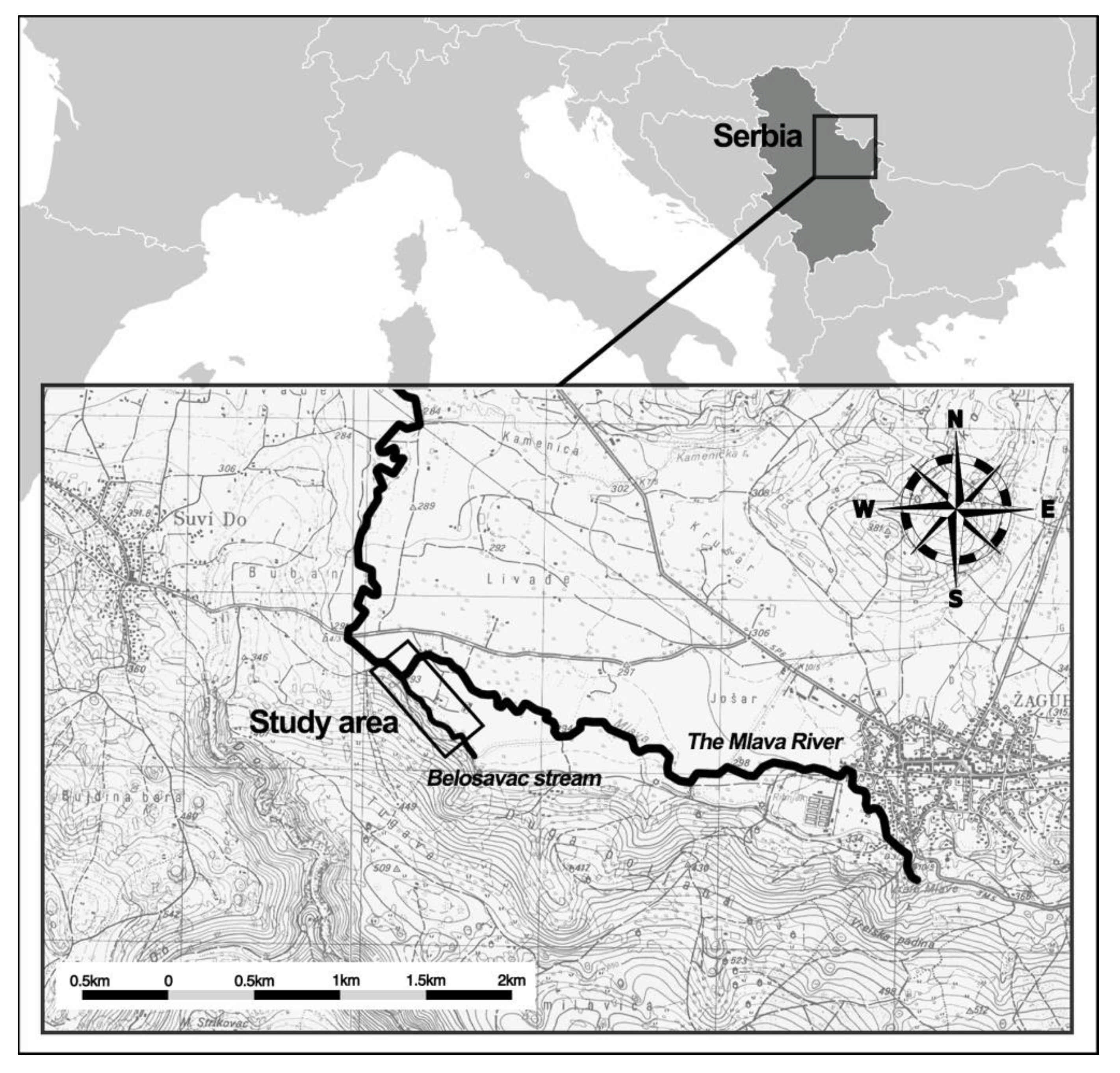
The study was carried out in eastern Serbia (Balkans) on a salmonid stream, Belosavac, a tributary of the Mlava River (N 44°12′03.0″, E 21°44′57.4″, altitude of 304 m, Figure 1). The Mlava River is the right tributary of the Danube, located in eastern Serbia. The Belosavac stream joins the Mlava River not far from its source.

The study was designed as a field experiment in the open hydrographic system of the Belosavac stream. The concept of the study was to examine the diet of a single population at one locality during one season. Fish and macroinvertebrates were sampled monthly in 2015 at the same locality from April to October. As live fish were handled for measuring and diet sampling, fieldwork was undertaken once a month so that the fish could completely recover between sampling rounds. The design included a comparison of the diet and availability of environmental prey (stream macroinvertebrates and terrestrial animals—insects, mollusks, arachnids, etc.) so that available prey were sampled at the same time as fish diet.

At the researched locality, the stream bed consists of large rocks (45%), gravel (45%), and sand (10%), as assessed during the study [28]. The stream is about 5 m wide, with a maximum depth of 100 cm measured in April on the researched stretch. The stream bed was 20–50% covered with vegetation predominantly consisting of the macrophyte Berula erecta (Huds.) Coville and was easily wadeable. The banks are flanked by willows (Salix spp.) and agricultural lowland grain fields and nearby plum orchards. The water was clear, with a temperature of about 11 °C with minor deflections; during the research period, the lowest temperature was measured in April (9.6 °C) and the highest in August and September (12.8 °C). Conductivity was in the range of 400–478 μS cm⁻¹, which is in accordance with the geology of the area (limestone). The water flow velocity of the stream was measured to be 0.3 to 0.6 m/s depending on the water level and macrophyte coverage during the period of research. Most of the fish were taken from the smaller wadeable stream Belosavac (250 m stretch) and the Mlava River along a short stretch (20–30 m) where the Belosavac joins it. Fish fauna was represented mainly by brown trout, rainbow trout (Oncorhynchus mykiss, Walbaum, 1792), chub (Leuciscus sp.), common minnow (Phoxinus phoxinus, Linnaeus, 1758), Danube barbel (Barbus balcanicus Kotlík, Tsigenopoulos, Ráb, and Berrebi, 2002), and bullhead (Cottus gobio, Linnaeus, 1758). All common groups of macroinvertebrate communities were present, with crustaceans from the Gammaridae family prevailing in abundance over other taxa.

2.2. Fish Measuring and Diet Sampling

A total of 232 fish individuals were caught during the research period. To collect fish, standard, battery-powered, backpack electrofishing gear was used. After measuring their size (standard length (SL) up to the nearest mm using a measuring tape, and weight (W) up to the nearest g using a digital scale), fish stomachs were flushed with clean water with a syringe and a silicone tube [29]. After processing, the fish were kept in a container with fresh aerated water until recovery and were subsequently released. The stomach content was extracted from each fish and stored in 70% alcohol.

2.3. Von Bertalanffy Growth Model, Condition Factor, and Length–Weight Regression

Fish age classes were determined for each month’s sample based on the curves of SL and W frequencies and from scales taken from brown trout in the field. From the mean SL values, von Bertalanffy growth parameters were calculated: L_∞ (maximal asymptotic length), t₀ (age at which scales start to grow), K (growth coefficient), and Φ’ (overall growth performance–growth quality) [30,31]. The condition factor (CF) [32] was calculated for each individual fish, and the mean CF was calculated for each age class and month as follows:

CF = (W/SL³) × 100,

(1)

with W being the weight (g) and SL being the standard length (cm). Each month’s sample growth was examined for isometry using linear regression of the log-transformed SL and W. The obtained regression coefficient b was then tested with the t-test to compare it with the isometric growth expected value (b = 3).

2.4. Macroinvertebrates from the Environment and Stomach Content

Benthic macroinvertebrates (macrozoobenthos) were collected by standard sampling with a benthological hand net (mesh size: 500 µm) from all available habitats (standard multihabitat sampling procedure), 10 subsamples taken according to habitat presence [28], referred to as a benthos sample. Drifting organisms were sampled with a drift net (frame size: 33 × 31 cm) placed in three locations on the studied stretch for 1 h. All macroinvertebrates from benthos and drift samples were counted and identified to the family, species, or genus level. Samples of extracted stomach contents were sorted, counted, and identified to the lowest possible level, and then damp-dried on a paper towel and weighed on an analytical balance with a sensitivity of 1 mg. The stomach contents were examined in the laboratory under a binocular stereomicroscope. Prey species were identified to various taxonomic levels depending on the taxon in question; terrestrial taxa were identified mainly to higher ranks than aquatic macroinvertebrates. Identified prey taxa were merged to fewer prey categories (30) for easier data management, analysis, and interpretation of results. All data were sorted by monthly samples of prey found in the diet and in the environmental samples. The data of consumed prey were sorted for the entire population and for age classes to calculate the indices of prey importance, diet diversity, diet overlap, electivity index, and Tokeshi’s graphical model.

2.5. Prey Importance and Diet Diversity

Prey importance and diet structure were analyzed using the abundance (A) of each prey type, frequency of occurrence (F), and index of relative importance (IRI). Diversity of diet was expressed with Simpson’s diversity index for age classes and for population by month. Abundance was calculated by the number and weight of consumed prey:

AN_i = (N_i/N_t) × 100 (%),

(2)

AW_i = (W_i/W_t) × 100 (%),

(3)

with N being the number of individuals of each consumed prey type (i) and N_t being the number of total consumed prey (for all fish of a subgroup, age class, or whole population). W is the weight of each consumed prey type (i), and W_t is the total weight of consumed prey (for all fish of age class or population).

Another parameter often used in prey importance assessment is the frequency of occurrence, which is calculated as the proportion of stomachs containing a certain prey:

F_i = (P_i/P_t) × 100 (%),

(4)

with P being the number of predators in which each prey type (i) occurred and P_t being the total number of predators.

Although the abundance and frequency of occurrence each can be used to assess prey importance in diet, the index of relative importance (IRI) integrates all three and is calculated as:

IRI = (AN% + AW%) × F%,

(5)

with AN being the abundance based on the number of prey, AW being the abundance based on the weight of the prey, and F being the frequency of occurrence [33,34].

Diet diversity (for fish subpopulation/individual fish) was tested with Simpson’s diversity index:

D = 1 − ΣN_i(N_i − 1)/N_t(N_t − 1),

(6)

value 0–1 (low–high), where N_i is the number of prey type i, and N_t is the total number of all prey items.

All calculations and graphs were performed in MS Excel 2010.

2.6. Importance of Terrestrial Prey in a Food-Rich Stream

Prey types were grouped into three major categories for the assessment of the importance of terrestrial prey, differentiated by their origin, benthos, terrestrial organisms, and flying adults of aquatic species. Although rare in samples, fish as prey was categorized as the fourth group. Brown trout prey on all of the abovementioned organisms. To estimate the importance of terrestrial prey in the diet of brown trout, this prey group was compared with aquatic adult and benthos prey proportions for each age class, in every month and for the whole population, using the AN, AW, F, and IRI indices. Selectivity toward terrestrial prey was also assessed for each prey type separately. All calculations and graphs were performed in MS Excel 2010.

2.7. Diet Overlap among Age Classes

Diet overlap was estimated by Pianka’s modification of the MacArthur and Lewin index [35], calculated as:

O = Σ(AN_ij × AN_ik)/sqrt(ΣAN_ij² × ΣAN_ik²),

(7)

where j and k represent the subgroups whose overlap is estimated, and AN is the proportion of the number of prey items of category i with O having the value 0 to 1 (low to high overlap).

2.8. Predation Selectivity

To analyze predation selectivity, the electivity index was used [36,37]. The electivity index is calculated based on Chesson’s coefficient (W_i) [24]:

W_i = (d_i/e_i)/Σ(d_i/e_i),

(8)

where d_i is the proportion of a certain prey type (i) in the diet, and e_i is the proportion of a certain prey type (i) in the environment (benthos/drift). When the W_i value is obtained, electivity is calculated as follows:

E = (W_i − 1/n)/(W_i + 1/n),

(9)

where n is the number of prey categories. E can range from −1 to +1, where −1 is negative selection or prey is unavailable to the predator, and +1 is positive selection. The calculation was performed in MS Excel 2010.

Foraging strategy was also assessed with Tokeshi’s graphical model [38] based on the diet diversity of age classes and population diet diversity data using Statistica for Windows (ver. 12).

2.9. Statistical Analysis

The unweighted pair-group average (UPGMA) method of hierarchical cluster analysis that used Euclidean distances was applied to determine the relationships between the age classes for different prey importance parameters (e.g., AN, AW, F, and IRI indices) and components (e.g., overall, Gammaridae, and terrestrials) of their diet in the research period. The program Statistica for Windows (ver. 12) was used for the analysis and making of figures.

3. Results

3.1. Fish Body Measurements and Growth Parameters

A total of 232 fish individuals were examined and measured; their SL and W were obtained and are presented for age classes (Table S1). The mean parameters of Bertalanffy’s growth model were as follows: L_∞ = 42.35 cm, t₀ = 0.57, and K = 0.36. Growth quality Φ’ was in the range 5.96–6.38 in monthly samples, which corresponded to the values expected for brown trout (6–6.5). The condition factor was lowest for age class 0+ and highest for the oldest classes (

Table 1. Condition factor (CF) of brown trout by age group and month.

Age Class	April	May	June	July	August	September	October	Mean CF for Each Age Class
0+	-	-	-	-	1.67	1.58	1.53	1.59
1+	1.49	1.82	1.65	1.81	1.71	1.64	1.45	1.66
2+	1.51	1.72	1.98	1.65	1.66	1.63	1.52	1.67
3+	1.67	1.74	1.85	1.79	1.62	1.84	1.56	1.73
4+	1.74	1.94	1.74	1.86	1.66	1.66	1.47	1.73
Mean CF for each month	1.60	1.81	1.81	1.78	1.67	1.67	1.51

). The mean condition factor was highest in late spring and during summer months (May, June, and July), and increased from age 1+ to 4+. Linear regression of the log-transformed SL and W was performed for all fish in the monthly samples. The R value was high (0.9), which shows that SL–W has a strong relationship. b≈3 indicates isometric growth, which was confirmed with the t-test (mean = 2.99, STDEV = 0.06, t-value −0.394, N = 7, p = 0.707, and the hypothesized mean of b is in the confirmation limits).

3.2. Benthos, Drift, and Diet Samples

All identified benthos and drift taxa (Table S2), as well as taxa determined as prey in diet samples, were merged into 30 prey categories (

Table 2. List of all identified prey taxa in diet samples of brown trout merged into 30 prey types.

Prey Type		Included Taxa
Benthic prey
1	Oligochaeta	Oligochaeta, Eiseniella tetraedra and others
2	Gammaridae	Gammarus sp.
3	Platyhelminthes and Hirudinea	Dugesia lugubris, Schmidt, 1861., Crenobia alpina, Dana, 1766, Erpobdella vilnensis, Liskiewicz, 1925
4	Mollusca	Pisidium sp., Ancylus sp.
5	Hydracarina	Hydracarina
6	Chironomidae and Simuliidae	Chironomidae and Simuliidae (larvae and pupae)
7	Limoniidae and Pediciidae	Eloeophila sp., Dicranota sp., Dicranoptycha sp. (larvae)
8	Tipulidae and Tabanidae	Tabanus sp., Tipula sp. (larvae)
9	Ephemeroptera larvae	Baetis sp., Heptagenia sp., Ephemera danica, Müller, 1764, Ephemerella sp.
10	Plecoptera larvae	Nemoura sp., Rhabdiopteryx sp.
11	Trichoptera larvae with cases	Beraeidae, Glossosoma sp., Potamophylax
12	Trichoptera larvae caseless	Lype sp., Plectrocnemia sp., Rhyacophila sp.
13	Aquatic Coleoptera and Heteroptera larvae	Limnius sp., Elodes sp., Elmis aenea, Dytiscidae (larvae)
Flying adults of aquatic prey (aerial adults)
14	Ephemeroptera adults	Baetis sp.
15	Trichoptera adults	Glossosoma sp., Lype reducta, Potamophylax luctuosus, P. latipennis, Silo nigricornis, Psychomyiidae
16	Aquatic Diptera adults	Chironomidae, Simuliidae, Dolichopodidae
17	Plecoptera adults	Plecoptera
18	Aquatic Coleoptera and Heteroptera adults	Limnius sp., Hydraena gracilis, Esolus angustatus, Elmis aenea, Pomatinus substriatus, Mesoveliidae
Terrestrial prey (adults and larvae)
19	Acari, Araneae, and Opiliones	Acari, Araneae, and Opiliones
20	Collembola	Collembola
21	Gastropoda	Gastropoda
22	Diptera	Muscidae and others
23	Coleoptera and Staphylinidae	Chrysomelidae, Cantharidae, Curculionidae, Coccinellidae, Scarabaeidae and others, Staphylinidae
24	Hymenoptera	Hoplocampa flava, Vespoidea, and others
25	Hymenoptera Formicidae	Formicidae
26	Heteroptera	Cicadomorpha and others
27	Dermaptera, Mecoptera, Psocoptera and Neuroptera.	Forficula auricularia, Linnaeus, 1758, Panorpa sp., Osmylus sp.
28	Lepidoptera larvae	Lepidoptera larvae
29	Orthoptera	Ensifera
Fish
30	Fish	Cottus gobio, Phoxinus phoxinus

) in order to calculate the proportion of consumed prey types, for each prey category, by age class and in total for each month (Table S4).

Benthos and drift samples revealed constant domination of Gammaridae in the environment and the presence of common benthic taxa and terrestrial organisms (Table S2). The macroinvertebrate community consisted of abundant Gammaridae with a seasonal average of 92%; Platyhelminthes, 2.55%; Chironomidae and Simuliidae, 1.92%; Mollusca 1.34%; Oligochaeta, 1.06%; Ephemeroptera, 1.01%; Coleoptera, 0.25%; and Trichoptera, 0.18%. Other groups contributed slightly, as assessed by analysis of standard benthos sampling. In the drift sample, the average seasonal proportions were somewhat different. Gammaridae were again the most abundant group with 93%. Ephemeroptera were present with 2.17%; Platyhelminthes, 2.09%; Chironomidae and Simuliidae, 1.89%; Coleoptera, 0.54%; Oligochaeta, 0.17%; Mollusca, 0.15%; and others had a lower share. Terrestrial organisms collected in the drift were Hymenoptera with 0.38% abundance; Collembola, 0.33%; Diptera, 0.19%; Araneae and Opiliones, 0.17%; and others. During the season, the proportions of different prey taxa varied. Those proportions were used to calculate the electivity index for each monthly sample.

To obtain improved resolution of the results, the 0+ age and fish with empty stomachs were excluded from diet analyses, as well as fish with fewer than five prey items, and 166 brown trout were included in the diet analysis. A total of 6913 individual prey items from diet samples were counted with a total wet weight of 91.07 g. The highest numbers and weights of prey consumed by one predator were recorded in May and September. The maximum number of prey items in one stomach was 361, found in an individual from the September sample (age 3+); the maximum weight of prey was 7.15 g in the stomach of an individual from the May sample (4+) (Table S3). In both individuals, almost the entire diet was composed of Gammaridae. The most abundant prey in the environment as well as in the total diet was Gammarus sp. (93.26% AN in the benthos and 90.50% AN in the drift; 78.85% AN and 79.97% AW in total analyzed diet).

3.3. Diet Description According to Number (AN) and Weight (AW) Abundance, Frequency of Occurrence (F), and Index of Relative Importance (IRI)

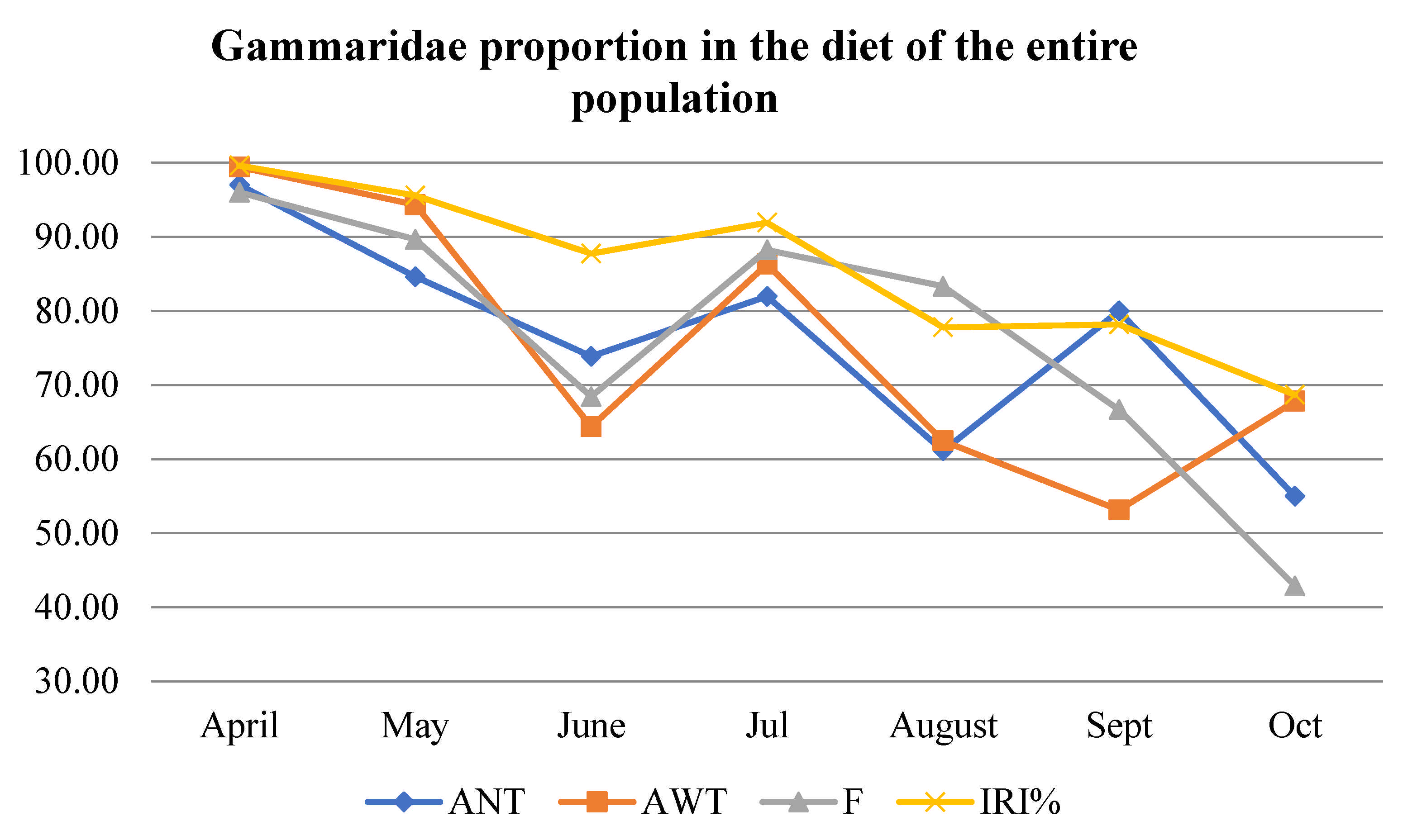
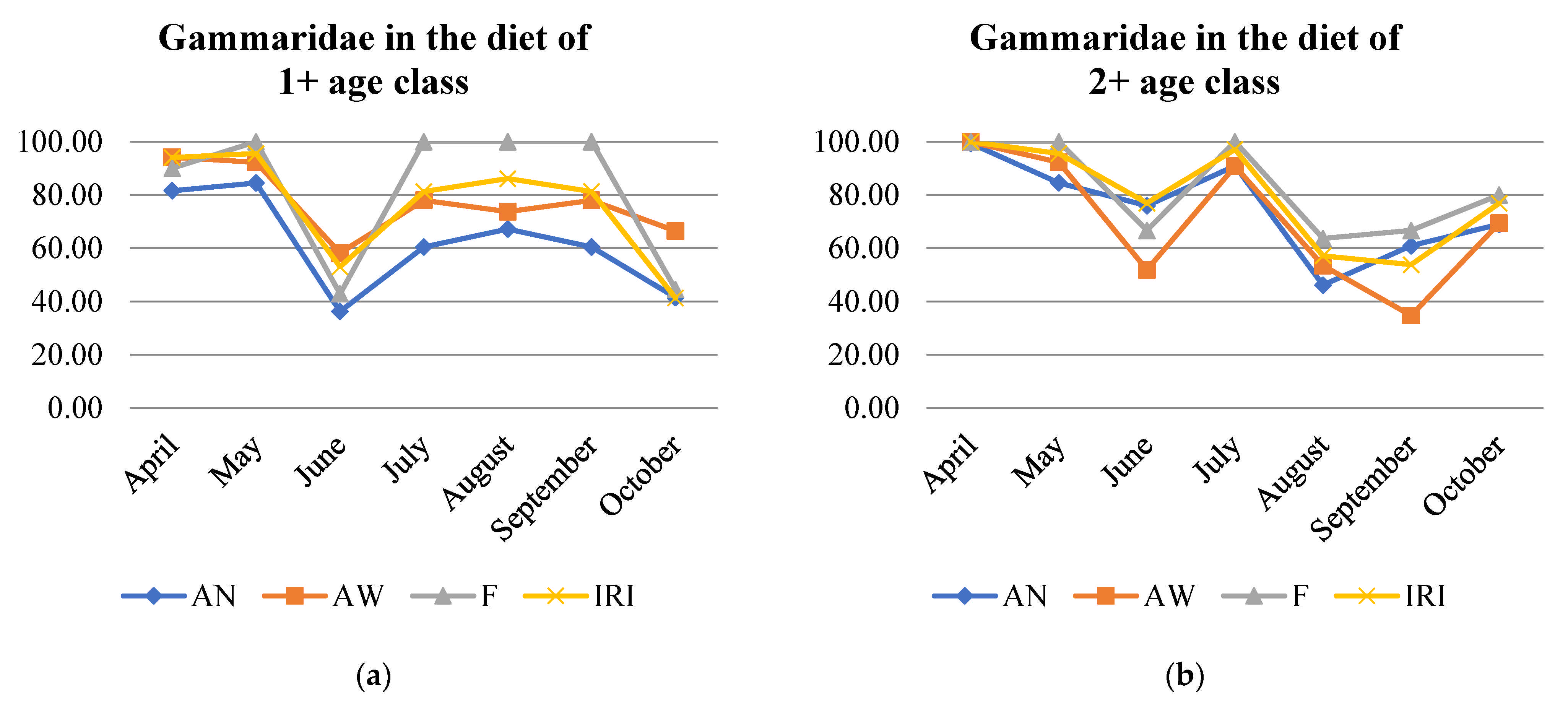
The importance of different prey types in the diet of brown trout of particular age classes (Table S4) and the most important five prey according to all indices for the population (

Table 3. The top 5 prey in the diet of brown trout at the population level, according to the AN, AW, F, and IRI parameters in % (only values for the first 5 prey for each month are shown).

AN	APR	MAY	JUN	JUL	AUG	SEP	OCT
Gammaridae	97.01	84.62	73.86	81.95	61.11	79.98	54.97
Ephemeroptera larvae	1.37	10.07	8.12	10.60	4.26	2.27
Plecoptera larvae	0.75
Chironomidae and Simuliidae	0.50	0.84		3.06	23.39	4.33	37.04
Trichoptera adult	0.12						2.14
Heteroptera		2.66		0.67
Coleoptera and Staphylinidae		0.35
Trichoptera with cases			5.84	1.15	4.91	3.22	1.17
Platyhelminthes and Hirudinea			3.81
Acari, Araneae, and Opiliones			1.27
Aq. Coleoptera and Heteroptera larvae					1.42
Formicidae						3.28
Dermaptera, Mecoptera, Psocoptera, and Neuroptera							0.97
AW	APR	MAY	JUN	JUL	AUG	SEP	OCT
Gammaridae	99.43	94.32	64.36	86.31	62.46	53.12	67.79
Plecoptera larvae	0.29
Ephemeroptera larvae	0.18	1.66		5.18
Chironomidae and Simuliidae	0.05			1.03	5.81		11.57
Trichoptera adult	0.03					2.42	3.91
Trichoptera with cases		1.24	16.61	2.39	21.79	21.90	12.54
Heteroptera		0.81		1.62
Trichoptera caseless		0.52			2.56
Platyhelminthes and Hirudinea			4.01
Phoxinus phoxinus			2.86
Cottus gobio						9.10
Oligochaeta			1.81
Muscidae					1.61
Formicidae						2.54
Tipulidae and Tabanidae							1.86
F	APR	MAY	JUN	JUL	AUG	SEP	OCT
Gammaridae	96	89.66	68.42	88.24	83.33	66.67	42.86
Ephemeroptera larvae	28	48.28	21.05	58.82	33.33	40.00
Plecoptera larvae	20
Chironomidae and Simuliidae	8	24.14		29.41	45.83	63.33	66.67
Trichoptera adult	4						9.52
Heteroptera		31.03
Trichoptera with cases			31.58	41.18	45.83	63.33	9.52
Trichoptera caseless		13.79
Platyhelminthes and Hirudinea			26.32
Acari, Araneae, and Opiliones			26.32			40.00
Formicidae				29.41
Aq. Coleoptera and Heteroptera larvae					20.83
Dermaptera, Mecoptera, Psocoptera and Neuroptera							14.29
IRI	APR	MAY	JUN	JUL	AUG	SEP	OCT
Gammarus	99.63	95.59	87.75	91.93	77.78	77.68	60.03
Ephemeroptera larvae	0.23	3.38	1.90	5.75	1.47	1.18
Plecoptera larvae	0.11
Chironomidae and Simuliidae	0.02	0.14		0.74	10.11	2.80	36.98
Trichoptera adult	0.003						0.66
Heteroptera		0.64
Trichoptera with cases		0.09	6.58	0.90	9.25	13.93	1.49
Trichoptera caseless					0.45
Platyhelminthes and Hirudinea			1.91
Acari, Araneae, and Opiliones			0.45
Formicidae				0.21		1.53
Tipulidae and Tabanidae							0.24

) revealed that Gammaridae were the most abundant prey, both in number and weight in almost all age classes and for every month. Age 4+ had a high consumption of Gammaridae during the entire period with a significant drop in September. The change in proportion of Gammaridae in the diet of the entire population throughout the research period from April to October exhibited a decreasing trend, from more than 90% in April to 50%–70% in September and October based on all four parameters (AN, AW, F, and IRI) (Table S4, Figure 2 and Figure 3), while the proportion of Gammaridae in the environment did not change. Cluster analysis showed that consumption of Gammaridae by age 4+ stood out by AN and AW, while by F and IRI 4+, it clustered together with age 2+ (Figure S1). April, May, and July clustered together as months with the highest Gammaridae consumption, while September and October stood out as months with the lowest consumption of this prey (AN, AW, F, and IRI) (Figure S2).

At the beginning of the season, Gammaridae constituted the major fraction of the trout population diet (>90%) but were preferred less by younger fish than by older fish (Table S4, Figure 3). At this time, brown trout of age 1+ had the most diverse diet, while those of age 4+ consumed only Gammaridae. Other prey favored during the early season were Ephemeroptera larvae (Baetis sp.) and, in smaller proportions, Plecoptera larvae and adults, Chironomidae and Simuliidae, and some terrestrial prey. Later, as more prey types became available, younger ages foraged on more different prey types, while brown trout of age 4+ still relied mostly on Gammaridae. Ephemeroptera larvae were consumed during the whole season, but highest consumption was observed from May to August and by younger ages. In early summer, diversification of diet was notable in ages 2+ and 3+, when the consumption of terrestrial prey became more prominent in all ages. While Gammaridae and Trichoptera with cases were the two principal prey in June, Platyhelminthes and Hirudinea were also consumed by all ages, with the highest proportion in the diet of 1+ and 2+ individuals. In August, consumption of Chironomidae and Simuliidae increased and remained in high proportion until the end of the season. Trichoptera with cases were most present in the diet during the summer months until September. Mollusca were consumed in late summer, with a peak in August. September was the month with the highest consumption of terrestrial prey in the population diet sample (Formicidae, Acari, Araneae, Opiliones, Coleoptera, and Staphylinidae). In October, Gammaridae and Chironomidae and Simuliidae had the highest share in the diet. Only in this month Tipulidae were present in the top 5 prey categories (Table 3 and Table S4).

The index of relative importance (IRI), which is calculated based on all three aforementioned parameters (AN, AW, and F) showed that apart of the dominant Gammaridae, several other groups were also important in the diet of brown trout. Prey types that represented more than 95% of the total diet in April and May were as follows: Gammaridae, Baetidae larvae, Plecoptera larvae and adults, Chironomidae and Simuliidae larvae, Trichoptera larvae (both with and without cases), terrestrial Heteroptera (Cicadomorpha) larvae, and some terrestrial Coleoptera adults and larvae. In the summer months, the most important prey were Gammaridae, Trichoptera larvae with and without cases, Chironomidae and Simuliidae, Ephemeroptera larvae, Platyhelminthes and Hirudinea, and terrestrials, such as Formicidae and Acari, Araneae, and Opiliones. In September and October, the important prey besides Gammaridae were Chironomidae and Simuliidae, Trichoptera larvae with cases, Ephemeroptera larvae, Formicidae, and Acari, Araneae, and Opiliones (Table S4). When the complete diet (according to IRI) was compared by age class, different results were exhibited during the research period. In the first months of the season, age 1+ separated and ages 2+ and 3+ clustered together, while in later months, ages 1+ and 3+ clustered together (Figure S3).

3.4. Terrestrial Prey

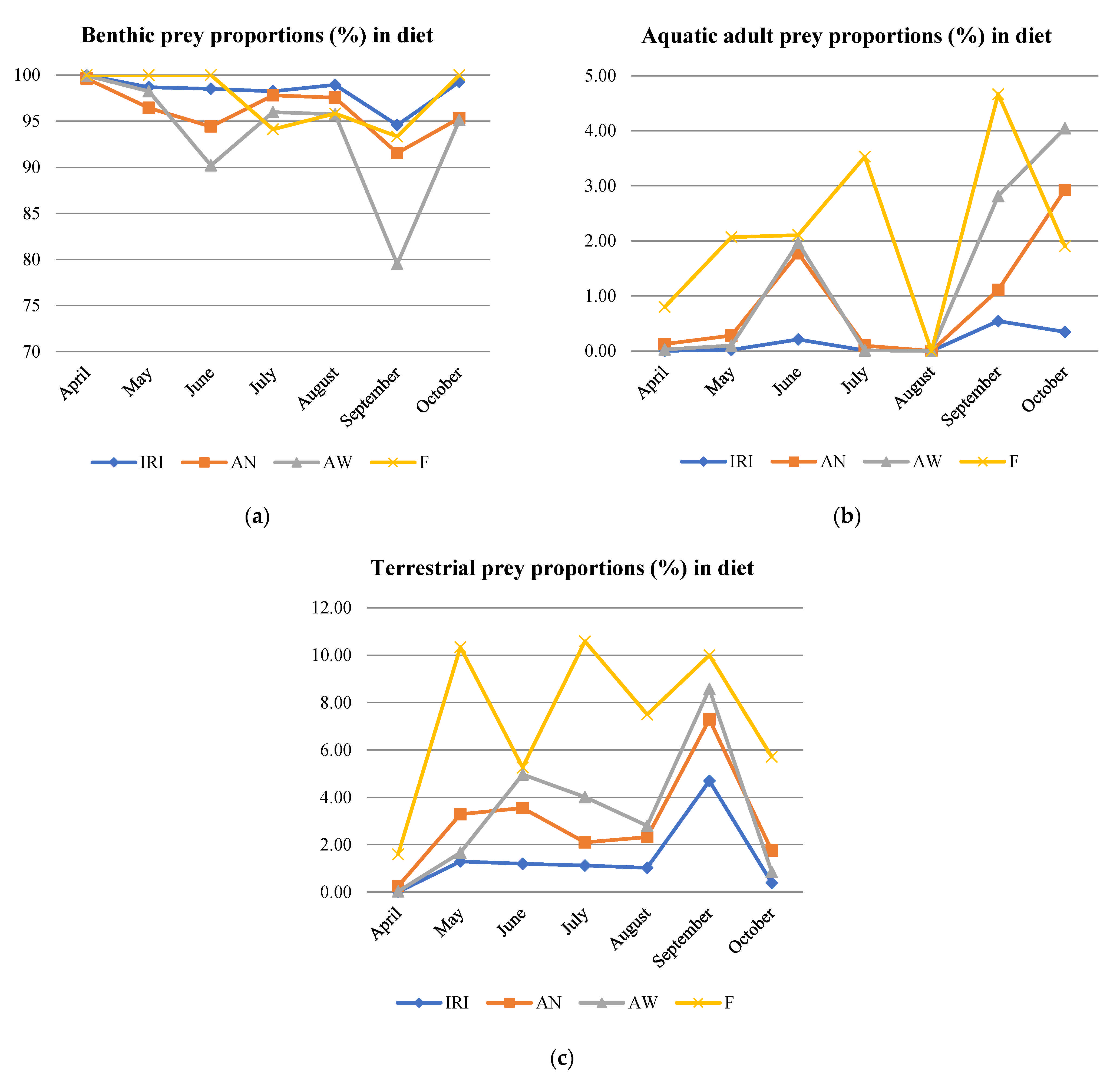
Higher ranks of prey types (benthic, aerial adults, terrestrial, and fish prey) were compared to assess the importance of terrestrial prey in the diet of brown trout. Benthic prey consumption was high throughout the season (AN, AW, F, and IRI), with a notable drop in September (AW), while aerial prey adults were present in very low proportions, but they increased toward the end of the season (Figure 4). Piscivory was recorded in June and August when Phoxinus phoxinus (common minnow) were found in the stomachs of two 2+ individuals. Those were young trout with body lengths of 16 cm in SL, 19 cm in TL, and 74 g in W, and of 18.7 cm in SL, 21.5 cm in TL, and 88 g in W. Additionally, a Cottus gobio (bullhead) was found in the stomach of one 1+ individual, of 13.6 cm in SL, 16.5 cm in TL, and 47 g in W, in September.

Terrestrial prey were present in the diet of brown trout during the entire period of research, with different proportions between age classes and in different months (Table S5, Figure 4). In April, terrestrial prey were absent in the diet of older individuals (3+ and 4+), but was present in the stomachs of younger trout (1+ and 2+). In May, terrestrial prey were present in the diet of all age groups, less in younger, more in older individuals, when expressed by number abundance (AN). However, when the weight abundance (AW) of the prey was considered, age groups 1+ and 2+ had a higher proportion of terrestrial prey than older ages (i.e., younger fish ate larger terrestrial prey). In June and July, terrestrial prey were present in the diet of all age groups, with the highest share in age 3+ (AN). In August, ages 2+ and 3+ consumed more terrestrial prey than ages 1+ and 4+. In September, terrestrial prey were present with the highest percentage, when the entire population was considered, according to the AN, AW, and IRI of all other monthly samples. In October, age class 3+ had the highest proportion of terrestrial prey (AN, AW, and IRI); however, for the whole population, the share of terrestrial prey was lower than in September. In general, terrestrial organisms were mostly consumed by brown trout of ages 2+ and 3+. According to AW, the greatest percentage of terrestrial prey was recorded in the summer months, with peaks in June and September. According to F values, half of the brown trout population consumed terrestrial prey in May, July, and September (Table S5). Even when considering each terrestrial prey type separately, they were present in the top 5 prey types along with Gammaridae and other aquatic prey.

When IRI was applied to the monthly population samples, the importance of terrestrial prey was very low from April to August (<2%), reaching peak consumption in September with 4.70%, and decreased in October (Table S5, Figure 4).

The electivity index generally revealed positive selection towards all terrestrial prey, with some minor exceptions and variations between monthly population samples (Table S6). Most favored prey were Acari, Araneae, Opiliones, Coleoptera, Staphylinidae, Formicidae, and Hymenoptera, while Heteroptera and Hymenoptera were both negatively and positively selected depending on the month and age group.

When age groups were considered, several conclusions could be made: Acari, Araneae, and Opiliones were positively selected by all ages and in all months, except August. Coleoptera and Staphylinidae were positively selected by ages 1+ and 2+. Formicidae were positively selected by age 1+ in April, by age 3+ in July, and by age 2+ in September. Hymenoptera were positively selected mostly by age 2+ and were negatively selected in July. Terrestrial Diptera were positively selected in September and October by ages 1+ and 2+ (Table S6).

The overview of terrestrial prey taxa present in the diet showed that the highest diversity of terrestrial prey was detected in June, July, and September. The prey types that were present in the diet during most months were as follows: Coleoptera and Staphylinidae; Acari, Araneae, and Opiliones; Hymenoptera (mainly Vespoidea); Heteroptera (Cicadomorpha adults and larvae); and Formicidae. When cluster analysis was applied, age 3+ separated from the other ages according to three indices (AN, AW, and IRI) as the age with the highest consumption of terrestrial prey (Figure S4). Comparison of the monthly population consumption of terrestrial organisms revealed that September also stood out as the month with the greatest importance for terrestrial prey (AN, AW, and IRI) (Figure S5).

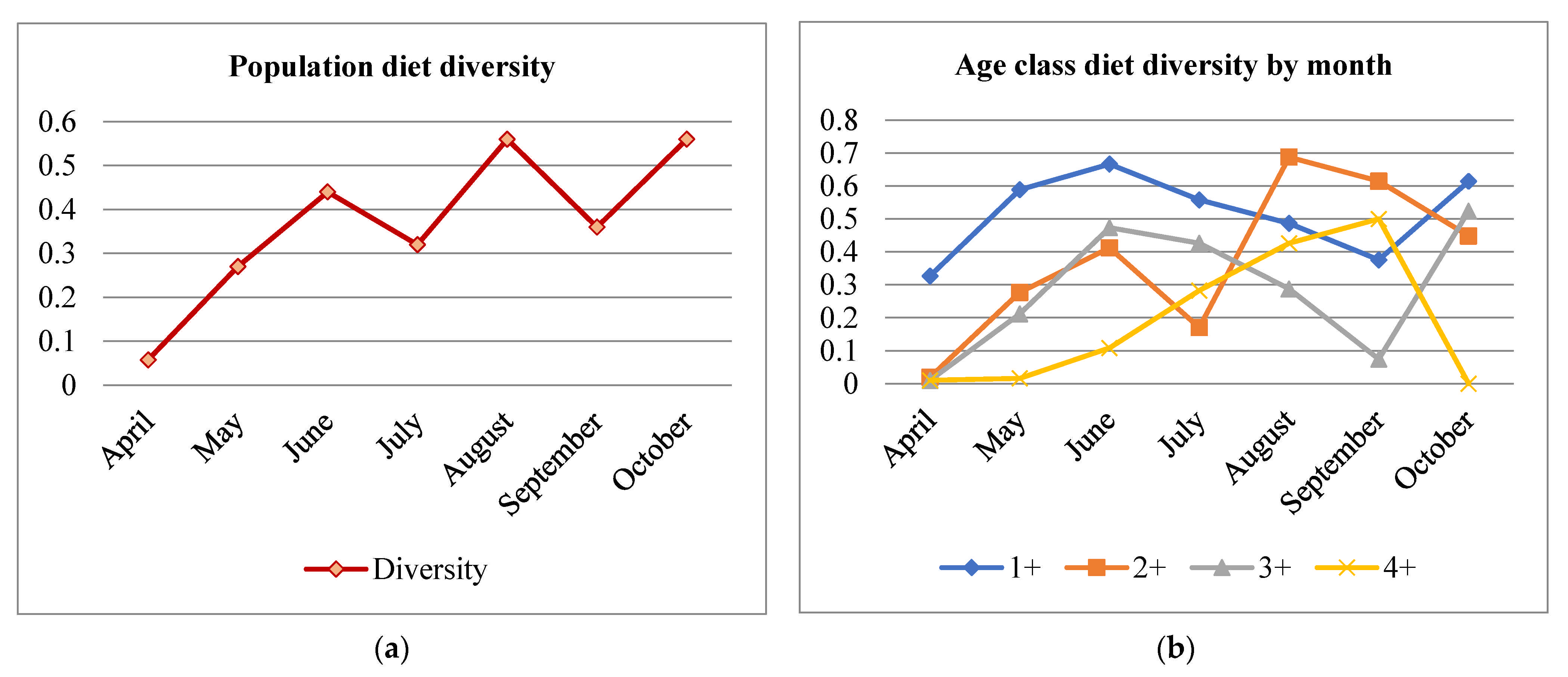
3.5. Diet Diversity

Diet diversity exhibited an overall increasing trend from April to October with peaks in June, August, and October with the highest diversity recorded in brown trout of the ages 1+ and 2+ (Figure 5).

3.6. Diet Overlapping among Age Classes

Overlap in diet was done for all possible relations in each month’s diet sample. For the whole research period, diet overlap among age classes was near 1. The lowest overlap in diet was in the months September and October in some of the relations (2+ and 3+, 3+ and 4+, 4+ and 1+, and 4+ and 2+) (

Table 4. Diet overlap between age classes; low overlapping is in bold font and shaded (0–1, low–high).

	1+ and 2+	2+ and 3+	3+ and 4+	4+ and 1+	4+ and 2+	1+ and 3+
April	0.99	1.00	1.00	0.99	1.00	0.99
May	0.84	0.99	0.99	0.78	0.99	0.78
June	0.64	0.99	0.99	0.62	0.99	0.62
July	0.93	0.99	0.99	0.94	1.00	0.93
August	0.95	0.84	0.98	0.98	0.90	0.95
September	0.93	0.98	0.16	0.16	0.21	0.91
October	0.89	0.36	0.00	0.67	0.01	0.72

).

3.7. Selectivity (Electivity and Tokeshi’s Graphical Model)

The electivity index was obtained separately for comparison of the diet and benthos sample (macrozoobenthos (mzb)) and the diet and drift sample. Mzb and drift were used to represent the proportions of prey types in the environment based on AN. Unfortunately, in none of the two, flying adults of aquatic insects were collected (due to their low number or absence at the moment of sampling). In the mzb sample, no terrestrial prey was present. The mzb prey, as well as the terrestrial prey, was present in the drift samples at different proportions so that the two were analyzed separately. For an easier comparison, the results are presented according to month, and in each month, mzb and drift were compared with the diet (Tables S6 and S7).

Even though Gammaridae were important prey in the diet and the most abundant prey, trout consumed them in proportions that were lower than in the environment (negative selection) for most of the period. Trout favored other present prey that were much less abundant than Gammaridae (positive selection). Gammaridae were positively selected only in April and October by the mzb sample, and selection was negative to neutral according to drift in all months (Table S6). Ephemeroptera larvae were positively selected throughout the season, by both mzb and drift environmental samples. Plecoptera were present and positively selected at the beginning of the season (April and May). Chironomidae and Simuliidae were positively selected at the end of the season, and earlier in older age groups. In general, Trichoptera with cases and caseless larvae were both positively selected from the midseason to its end, with some differences observed between mzb and drift samples. Mollusca were positively selected only in August (drift) and September (mzb and drift) even if they were present in the environment throughout the entire season. All terrestrial prey were positively selected except Heteroptera in samples in June and August; Hymenoptera, Diptera, and Lepidoptera in July; and Acari, Araneae, Opiliones and Diptera in August. Oligochaeta and Platyhelminthes and Hirudinea were negatively selected, by both the mzb and drift at the population level. Aquatic Coleoptera and Heteroptera larvae and adults were mainly negatively selected (all months by drift), with positive selection in August, September, and October (mzb). Limoniidae and Pediciidae, as well as Tipulidae and Tabanidae, were mostly negatively selected, with some exceptions at the end of the season (Table S6).

Differences in the selectivity of predation in age classes for several important prey are presented in

Table 5. Electivity of the most important prey types in the diet; positive (+, >0.3), neutral (0, −0.3–0.3), and negative (−, <−0.3) selection.

Gammaridae		APR	MAY	JUN	JUL	AUG	SEP	OCT
1+	MZB	0	-	-	-	-	-	-
	Drift	-	-	-	-	-	0	-
2+	MZB	+	-	-	-	-	-	-
	Drift	+	-	-	0	-	-	-
3+	MZB	+	-	-	-	-	+	-
	Drift	+	+	-	-	-	0	-
4+	MZB	+	+	-	+	-	+	+
	Drift	+	+	+	+	-	-	+
Chironomidae and Simuliidae		APR	MAY	JUN	JUL	AUG	SEP	OCT
1+	MZB	+	0	-	-	-	0	+
	Drift	-	-	-	+	+	+	+
2+	MZB	-	-	0	-	-	0	+
	Drift	-	-	0	-	+	+	+
3+	MZB	-	-	-	-	-	0	0
	Drift	-	-	-	-	+	+	+
4+	MZB	-	-	-	-	-	-	-
	Drift	-	-	-	0	0	-	-
Ephemeroptera larvae		APR	MAY	JUN	JUL	AUG	SEP	OCT
1+	MZB	+	+	+	+	+	+	+
	Drift	-	+	+	+	0	+	+
2+	MZB	0	+	+	+	+	+	+
	Drift	0	0	0	0	0	+	+
3+	MZB	0	0	/	+	+	+	/
	Drift	0	+	-	0	-	+	/
4+	MZB	-	0	-	+	-	/	/
	Drift	-	0	-	+	-	-	/
Trichoptera with cases		APR	MAY	JUN	JUL	AUG	SEP	OCT
1+	MZB	-	/	+	0	+	+	0
	Drift	-	-	+	+	0	0	-
2+	MZB	-	+	+	-	+	+	+
	Drift	-	0	+	0	+	+	-
3+	MZB	-	/	+	+	+	+	-
	Drift	-	-	+	+	+	+	-
4+	MZB	-	/	+	-	-	+	-
	Drift	-	-	+	-	-	+	-
Trichoptera caseless		APR	MAY	JUN	JUL	AUG	SEP	OCT
1+	MZB	-	0	+	+	+	+	+
	Drift	/	+	+	+	+	0	-
2+	MZB	-	+	-	+	+	+	/
	Drift	/	0	-	+	+	0	-
3+	MZB	-	-	+	/	-	-	/
	Drift	/	-	+	-	-	0	-
4+	MZB	-	+	-	/	-	+	/
	Drift	/	+	-	-	-	+	-
Acari, Araneae, and Opiliones		APR	MAY	JUN	JUL	AUG	SEP	OCT
1+	MZB	/	/	/	/	/	/	/
	Drift	/	/	+	+	-	0	/
2+	MZB	/	/	/	/	/	/	/
	Drift	+	+	+	-	-	+	+
3+	MZB	/	/	/	/	/	/	/
	Drift	/	/	+	+	-	-	/
4+	MZB	/	/	/	/	/	/	/
	Drift	/	/	+	+	-	-	/
Coleoptera and Staphylinidae		APR	MAY	JUN	JUL	AUG	SEP	OCT
1+	MZB	/	/	/	/	/	/	/
	Drift	/	+	-	+	/	+	+
2+	MZB	/	/	/	/	/	/	/
	Drift	/	+	/	/	+	+	/
3+	MZB	/	/	/	/	/	/	/
	Drift	/	/	0	/	/	/	/
4+	MZB	/	/	/	/	/	/	/
	Drift	/	/	-	/	/	/	/

, and in detail for each age group in Table S7. Ephemeroptera larvae were present in the diet of all age groups but prevailed in younger fish throughout the season. Trichoptera larvae were also positively selected by all age groups. Younger ages, 1+ and 2+, expressed neutral to negative selection towards Gammaridae and favored other benthic and terrestrial prey and had a very diverse diet. Age 3+ also had a heterogenous diet and positively selected prey that were usually negatively selected, such as Mollusca, Platyhelminthes, and Hirudinea. Age 4+ mainly positively selected Gammaridae, Trichoptera larvae with cases and sometimes Platyhelminthes and Hirudinea, and occasionally other benthic prey. Terrestrial prey were more favored by ages 1+, 2+, and 3+ than by age 4+ (Table 5 and Table S7).

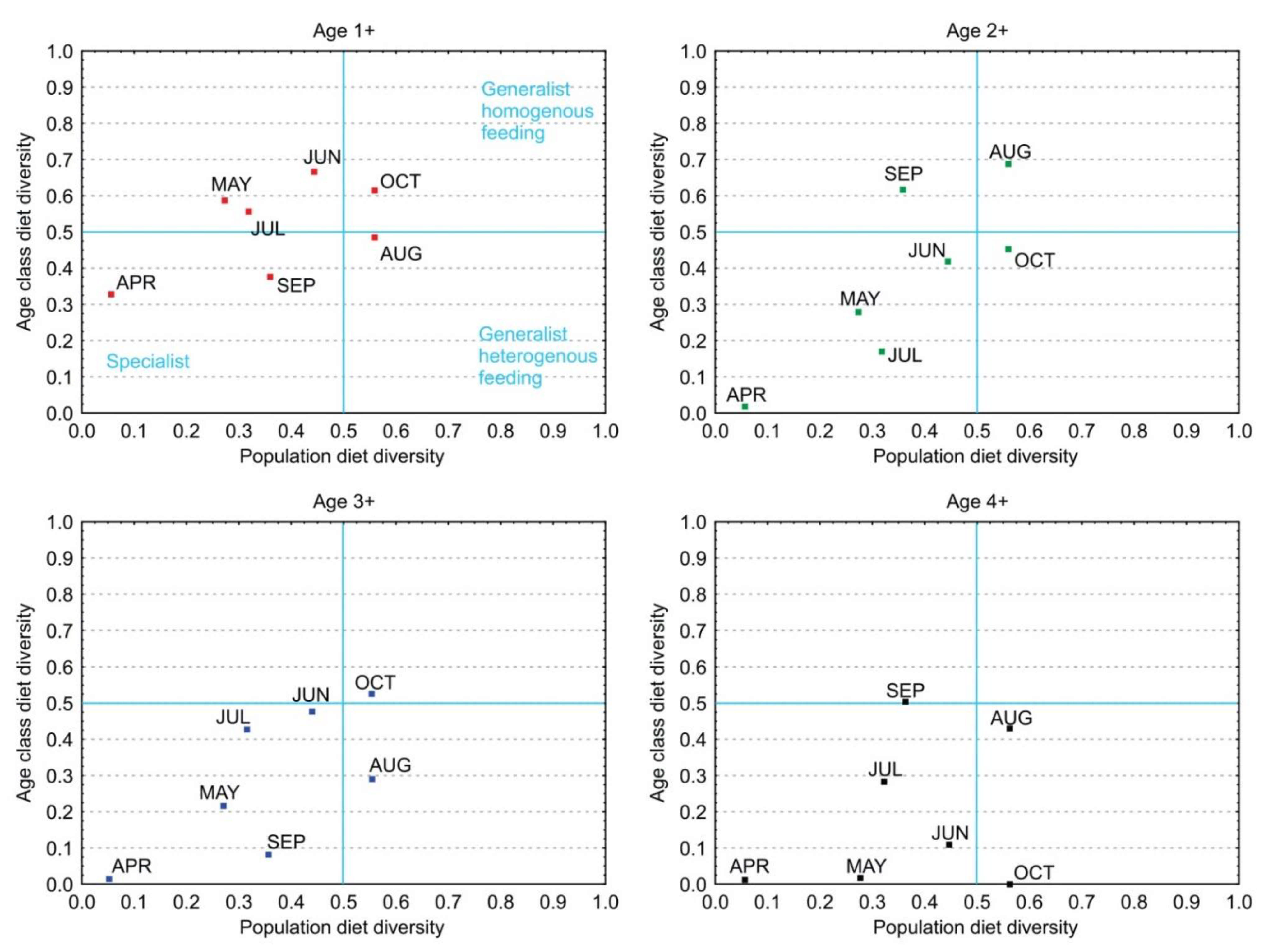
Tokeshi’s graphical model was obtained based on the diet diversities of age classes 1+ to 4+ and the population diet diversities in the period April to October. Each age is presented in a separate graph in Figure 6. On the right side of the graphs are entities that are considered generalists, and a true specialist is positioned in the lower left quadrant, with low individual (age class diversity) and population diversities, while the upper left quadrant represents transition from a specialist to a generalist strategy. Age 1+ had the highest diet diversity and displayed a transition to a generalist strategy, while others were positioned mainly in the lower left quadrant showing selective feeding with a low diet diversity and were considered specialists with homogenous feeding.

4. Discussion

There are many studies of salmonid fish diet, which have all revealed the great feeding plasticity of brown trout that depends to a large extent on local habitat characteristics [3,5,6,8,10,14,20]. This study provides insight into the complex brown trout feeding habits during one season at a locality that can be considered an example of a food-rich limestone stream. Application of four prey importance indices, two selectivity assessment approaches, diet diversity, and diet overlap for different age classes and population levels provided new inferences and perspectives. Good growth of brown trout based on growth quality (Φ’) and CF was confirmed, and the diet variations of age classes were observed using prey importance indices and diet diversity. Younger ages showed higher diversification of the diet in contrast to older individuals. Terrestrial and other rare prey were relevant and positively selected in the brown trout diet, even in a stream very rich in aquatic macroinvertebrates.

In the present work, diet sampling was performed by syringe flushing, which was chosen as an easy and inexpensive method for extracting the stomach content while keeping the fish alive, allowing for repetitive sampling at the same locality. An additional advantage of this method is that the stomach content is not digested as it is usually in the distal part of the digestive tract. Sampling of the prey that were available in the environment was performed by two approaches, standard benthos sampling and drift sampling. The more useful environmental sample that was compared with the diet samples was the drift sample. It collects macroinvertebrates from the benthos, aquatic areal adults, and terrestrial organisms that fall in the water, and thus includes all available brown trout prey types. Prey availability was analyzed in some studies, and the level of availability was consonant with the tendency of prey to drift, both actively and passively [4,5,10,39].

Brown trout benefits from all stream characteristics of this chalk stream rich in food, with a stable water level and flow, stable temperature, and good habitat heterogeneity. Owing to the abundance of Gammaridae, there was no food scarcity. During the research period, Gammaridae were the dominant prey in the environment and in the diet. This prey was most important at the beginning of the season when other prey were in low numbers. From month to month, they were dominant in both the diet and the environment. However, other prey became more available and more favored, as revealed by the decreasing proportion of Gammaridae in the diet from April to October.

The richness of the available food, as well as the good growth of trout, was confirmed by the growth quality parameter (Φ’), which corresponded to values expected for brown trout and high (>1.5) CF for the whole population in all months. The lowest values of the CF were observed in spring when the available food was less diverse; as the season progressed, more food became available (more terrestrial prey, more flying adults). Hence, the highest CF values were recorded in the summer months. As the end of the season approaches, many insect groups complete their life cycles, and brown trout prepares for spawning, and the CF slightly decreases. The mean CF ascended from age 1+ to age 4+, which can be explained by older fish gaining more in weight than in length compared with younger fish in an environment where they do not encounter food shortage. Similar results for high CF were reported in Alp et al. [7] for a higher number (10) of age classes. However, the authors did not report an increase in CF from younger to older ages. Additionally, from May to February, when their study was performed, the CF had lowest values in May and June and afterwards remained near a value of 1.5.

To analyze prey importance, three parameters, AN, AW and F, and one index that integrates all three, the IRI index, were used. Prey number (AN) tells us about how many times fish foraged for each prey item; therefore, this parameter describes the intent of fish to forage for a specific type of prey. On the other hand, the parameter prey weight (AW) shows what quantity of each food is consumed and in what proportion to other food. A single prey item can have more weight than dozens of other smaller ones. When F is analyzed, we can estimate what prey trout (as a specified age group, subpopulation, etc.) will pay particular attention to; therefore, we can conclude that most of the fish in the group will pursue a prey of a certain type if F is greater than 50%. Finally, IRI integrates all of the given parameters to extricate a few important prey types from all available ones [40]. Similarity in proportions of AN and AW showed that brown trout foraged for prey of uniform size and weight, with some exceptions for prey items that had higher proportions by weight than by number, such as Trichoptera larvae, Platyhelminthes and Hirudinea, terrestrial Coleoptera, Tipulidae and Tabanidae, Lepidoptera larvae, and fish prey. According to the IRI, the prey that were shown to be important were Gammaridae, Ephemeroptera larvae, Chironomidae and Simuliidae (larvae, pupae, and adults), Trichoptera larvae, Plecoptera, Platyhelminthes and Hirudinea, terrestrial Heteroptera, Coleoptera, Formicidae, and Araneae at different proportions in different months. Resolution of the results was skewed toward Gammaridae in all analyses because of their high abundance. Nevertheless, even though other prey items were in significantly lower proportions, they were appealing to brown trout, which was also confirmed by the electivity index. It seems that Gammaridae were less important for younger ages (1+ and 2+). Higher consumption of Gammaridae by older fish could be due to intraspecific competition for the most preferable microhabitat. The authors stated that older brown trout prefer deeper and slower zones of the habitat [41,42], and different habitat utilizations by different age groups for feeding can contribute to food resource partitioning [10]. Other studies have examined and discussed territoriality and the positioning in riffles and pools and their effect on diet differences between sex and age groups in different microhabitats, which also support this statement [3,10,11]. Consequently, the available food would be different for differently positioned fish. Older fish (4+) occupy slow-flowing water in the deepest zones of the river that have less diverse benthos prey, but are rich in Gammaridae at this locality, while younger fish are forced to inhabit shallower areas and to consume the prey available there. In the shore zone, different prey, including terrestrial, are more accessible; this can explain why age 1+ displayed a more diverse diet and a transition to a generalist strategy (Tokeshi’s model).

Sánchez-Hernández and Cobo [10], Kara and Alp [6], and Alp et al. [7] confirmed that benthic organisms (i.e., their larvae, pupae, and adults that live on the riverbed and drift in the water column) are the most foraged prey of brown trout, as also confirmed in this study. Additionally, adults of some aquatic insect groups hatch and mate near water and lay eggs on the water surface or beneath it and then become available to brown trout as prey. Terrestrial organisms end up in the water, carried by the wind and rain runoff, falling in the water from shore vegetation, while swarming near the shore, and so forth. All of these are not as abundant as benthic prey but are easily available to brown trout. The importance of terrestrial prey for salmonids has been confirmed in several studies [43,44,45,46]. During the research period, benthic organisms were the most consumed prey, with the lowest values in September when terrestrial prey had the highest share. The proportion of terrestrial prey in the diet showed an increasing trend from April to September. Whenever terrestrial prey (e.g., Formicidae, Araneae, or Cicadomorpha) was present, it was mainly positively selected and was present in the diet of almost all age groups in all months. Terrestrial prey (individually) proved to be important according to prey importance indices by being present in the top 5 prey types in almost all months despite a low environmental presence in comparison with benthic prey. Sánchez-Hernández et al. stated that the increase in fish size is accompanied by an increase in the proportion of terrestrial prey in the diet [10]. In our study, terrestrial prey was the most important at ages 1+, 2+, and 3+, but the least at age 4+. It has been to pointed out that older fish (4+) also showed interest in terrestrial prey in September, which coincided with lower consumption of Gammaridae. The importance of terrestrial prey in the diet of brown trout living in a food-rich salmonid stream could be due to the higher energy gain from catching easy prey and diet diversification, and/or it could have a behavioral aspect (i.e., if the prey is rare, it attracts attention). The underlying reason for the selection of rare prey could be synergy in avoiding the confusion effect in foraging on abundant prey, and an oddity effect where rare prey is concerned, as foraging of an aggregation of prey can cause sensory confusion, while a single rare organism can be more conspicuous to the predator, as is the case in coral reef fish [47]. This observation may be applicable to brown trout as well. Among these rare preys, there are also those that are of aerial or terrestrial origin, which are slower or immobile in the water medium and, as such, are easy to catch. Such prey yield a fair amount of energy with minimal effort. Another explanation for the apparent selectivity for terrestrial invertebrates is probably the greater foraging efficiency during daylight hours, which coincides with the greatest input of terrestrial invertebrates to streams occurring during daylight hours. Terrestrial prey also tends to be larger than aquatic prey, which is why it can be more conspicuous to fish [48].

Flying adults from aquatic insect groups were present in very low proportions as prey in all months, but they were absent in the environment during fieldwork. As each sampling day had its specificities (e.g., wind, water temperature, and occurrence of hatches) that can influence trout foraging for surface prey, the relatively low proportion of airborne insect prey in all months was most likely related to their absence in the environment during field sampling.

Piscivory was recorded in only three individuals that preyed on Phoxinus phoxinus and Cottus gobio. Some authors have stated that piscivory in brown trout usually starts when a body length of 20–30 cm is attained [16,17]. In this research, piscivory was shown to exist even in younger fish of shorter length.

When the entire population was considered, diet diversity was lowest at the beginning of the season, increasing until the season’s end. In all months, age 1+ exhibited the highest diet diversity (and lowest interest in Gammaridae). Only in August and September did brown trout of 2+ age had the highest diet diversity. Brown trout of 4+ age had the lowest diet diversity in general, with a peak in diversity in September. Low diet diversity at the beginning of the season is probably the consequence of low environmental diversity. The diet diversity in the 1+ age class was high, with individuals positively selecting Ephemeroptera larvae; Trichoptera larvae (predominantly caseless ones); Plecoptera, Chironomidae, and Simuliidae; and the larvae of aquatic Coleoptera and some terrestrial prey in low proportions. Age 2+ diet was similar to age 1+ diet, but with the addition of positively selected Formicidae, Heteroptera, Dermaptera, Lepidoptera larvae, and Araneae. Even though the number of prey types consumed by 2+ was somewhat higher than that for age 1+, diet diversity was lower in 2+ than in 1+ because Gammaridae had a much higher proportion than other prey (lower evenness). Age 3+ and especially age 4+ had lower diet diversities than the younger ages. The whole population and each age class had a more diverse diet from month to month as different prey items became available. Generally, overlap in diet between brown trout of different ages was high, as expected in an environment with relatively low prey diversity and a domination of Gammaridae. Lower grade overlap was observed later in the season, when more different prey types were available.

According to the results of the electivity index, Gammaridae were negatively selected for most of the research period and were occasionally neutral or slightly positive. Nevertheless, they have predominance in the diet of trout due to their great abundance in the environment. In most months, Ephemeroptera and Trichoptera larvae were positively selected, as well as Chironomidae and Simuliidae in the second half of the season when terrestrial prey was also positively selected. It is interesting that in the River Nera, negative preference for Ephemeroptera was observed for all ages, which is in contrast to our findings, as well as positive selection for Trichoptera larvae for fish younger than 4 years [25].

According to Tokeshi’s graphical model for estimating foraging strategy, all age classes were positioned in the lower left quadrant of the graph, so their strategy can be considered specialist, with low population diet diversity and low mean age class diversity, while age class 1+ expressed a more diverse diet compared with other age groups and a tendency towards a generalist strategy. Age 4+ had the lowest values for diet diversity during most of the season.

Rosenbauer suggested that a fly fisher should pay attention to geology when ‘reading’ a river before casting a fly [26,49]. Simonović et al. showed that the geological structure of a stream’s bedrock has an important effect on the character of a trout stream and fish feeding habits [50]. If the stream flows over an insoluble bedrock (e.g., granite), it will be less fertile in terms of available food, and trout will be smaller and will fight for food vigorously. If it flows over limestone, a highly soluble rock, the water will be of high conductivity, which enhances the production of prey [26,45]. Such a stream will be richer in prey, and brown trout will grow bigger [46]. According to this, the stream we researched can be characterized as rich with life. When the results obtained from this study are applied to fly fishing, we could say that brown trout in April and May should select Baetis larvae, Plecoptera nymphs and adults, terrestrial Coleoptera, and Heteroptera (Cicadomorpha). Ephemeroptera larvae are a prey selected from April to July and even longer, Formicidae from July to October, cased Trichoptera larvae (Potamophylax sp.) from July to October, and Chironomidae and Simuliidae from August to October. Even though flying adult prey were not captured by drift sampling owing to their rare occurrence in the environment, they were present in the diet. Thus, if any dense hatch or mating adults’ fall is present and provokes brown trout to feed at the surface, then the deceivers of the proper stage (emergers, pupae, duns, or spinners) should be applied. On the other hand, Araneae and Opiliones were present in the top 5 types of prey in all months. Additionally, other types of prey that were present in the diet could be tempting for brown trout from the mid- to late season and would include Vespoidea, Forficula sp., Ensifera, Panorpa sp., Tipulidae, and Lepidoptera larvae. Brown trout positively selects many terrestrial prey types, perceiving them as either large and conspicuous or helpless and easy to catch in the aquatic environment. Hence, in the absence of dense hatches, it would be worth casting them as generalized attractors, especially on windy days or after rain showers.

5. Conclusions

Brown trout is a predator with great feeding plasticity and dietary shifts throughout ontogeny. Trout display different foraging strategies during the season and quickly respond to changes in the environment and prey availability. Terrestrial prey has an important role in their diet, as well as other rare prey types. They behave selectively toward a variety of prey all the time, either negatively or positively, and for some prey types, the direction and level of selection change over the season. Habitat characteristics and prey dynamics (i.e., availability) have considerable influence on the feeding habits of brown trout.

The growth of brown trout was respectable with a high condition factor that was recorded in all age classes and in all months as a result of a food-rich environment. Diet variations in different age classes over seasonal scales were observed and described by four prey importance indices and diet diversity. Population diet diversity increased from the beginning to the end of the season. Ages 1+ and 2+ showed higher diet diversity than ages 3+ and 4+. Age 4+ had lower diet diversity than other age groups during most of the season except in August and September, and high consumption of Gammaridae during the entire period, which significantly declined in September.

The diet structure from April to October changed according to the seasonal change in prey availability. At the beginning of the season, the prey was less diverse; diet diversity then rose during the second part of the season when more terrestrial prey became available. The importance of terrestrial prey in the environment was confirmed by the positive selection of this type of prey, the values of indices of prey importance (especially frequency of occurrence), and their presence in the top 5 prey in the diet, especially considering the low environmental proportion of these types of prey.

In future studies, the obtained results will be compared with findings from similar habitats, rich limestone salmonid streams, and streams with different food richness and availability. The study could be improved with additional field experiments at the time of massive hatches, which would contribute to the establishment of feeding behavior during these specific events.

References

- Elliott, J.M. Quantitative Ecology and the Brown Trout; Oxford University Press: Oxford, UK, 1994; Volume 64, p. 301. ISBN 0198546785. [Google Scholar]
- Elliott, J.M. The food of trout (Salmo trutta) in a Dartmoor stream. J. Appl. Ecol. 1967, 4, 59–71. [Google Scholar] [CrossRef]
- Bridcut, E.E.; Giller, P.S. Diet variability and foraging strategies in brown trout (Salmo trutta): An analysis from subpopulations to individuals. Can. J. Fish. Aquat. Sci. 1995, 52, 2543–2552. [Google Scholar] [CrossRef]
- De Crespin De Billy, V.; Usseglio-Polatera, P. Traits of brown trout prey in relation to habitat characteristics and benthic invertebrate communities. J. Fish Biol. 2002, 60, 687–714. [Google Scholar] [CrossRef]
- De Crespin De Billy, V.; Dumont, B.; Lagarrigue, T.; Baran, P.; Statzner, B. Invertebrate accessibility and vulnerability in the analysis of brown trout (Salmo trutta L.) summer habitat suitability. River Res. Appl. 2002, 18, 533–553. [Google Scholar] [CrossRef]
- Kara, C.; Alp, A. Feeding habits and diet composition of brown trout (Salmo trutta) in the upper streams of River Ceyhan and River Euphrates in Turkey. Turkish J. Vet. Anim. Sci. 2005, 29, 417–428. [Google Scholar]
- Alp, A.; Kara, C.; Büyükcapar, H.M. Age, growth and diet composition of the resident brown trout, Salmo trutta macrostigma Dumeril 1858, in Fırnız Stream of the River Ceyhan, Turkey. Turkish J. Vet. Anim. Sci. 2005, 29, 285–295. [Google Scholar]
- Montori, A.; De Figueroa, J.M.T.; Santos, X. The Diet of the Brown Trout Salmo trutta (L.) during the Reproductive Period: Size-Related and Sexual Effects. Int. Rev. Hydrobiol. 2006, 91, 438–450. [Google Scholar] [CrossRef]
- Frank, M.; Piccolo, J.J.; Baret, P.V. A review of ecological models for brown trout: Towards a new demogenetic model. Ecol. Freshw. Fish 2011, 20, 167–198. [Google Scholar] [CrossRef]
- Sánchez-Hernández, J.; Cobo, F. Summer differences in behavioral feeding habits and use of feeding habitat among brown trout (Pisces) age classes in a temperate area. Ital. J. Zool. 2012, 79, 468–478. [Google Scholar] [CrossRef] [Green Version]
- Giller, P.; Greenberg, L. The relationship between individual habitat use and diet in brown trout. Freshw. Biol. 2015, 60, 256–266. [Google Scholar] [CrossRef]
- Poff, N.L.; Huryn, A.D. Multi-scale determinants of secondary production in Atlantic salmon (Salmo salar) streams. Can. J. Fish. Aquat. Sci. 1998, 55, 201–217. [Google Scholar] [CrossRef]
- Gerking, S.D. Feeding Ecology of Fish, 1st ed.; Elsevier: San Diego, CA, USA, 1994; ISBN 9781483288529. [Google Scholar]
- Keeley, E.R.; Grant, J.W.A. Prey size of salmonid fishes in streams, lakes, and oceans. Can. J. Fish. Aquat. Sci. 2001, 58, 1122–1132. [Google Scholar] [CrossRef]
- Keeley, E.R.; Grant, J. Allometry of diet selectivity in juvenile Atlantic salmon (Salmo salar). Can. J. Fish. Aquat. Sci. 1997, 54, 1894–1902. [Google Scholar] [CrossRef] [Green Version]
- Kahilainen, K.; Lehtonen, H. Brown trout (Salmo trutta L.) and Arctic charr (Salvelinus alpinus (L.)) as predators on three sympatric whitefish (Coregonus lavaretus (L.)) forms in the subarctic Lake Muddusjärvi. Ecol. Freshw. Fish 2002, 11, 158–167. [Google Scholar] [CrossRef]
- Jensen, H.; Bøhn, T.; Amundsen, P.A.; Aspholm, P.E. Feeding ecology of piscivorous brown trout (Salmo trutta L.) in a subarctic watercourse. Ann. Zool. Fenn. 2004, 41, 319–328. [Google Scholar]
- Vøllestad, L.; Andersen, R. Resource partitioning of various age groups of brown trout Salmo trutta in the littoral zone of Lake Selura, Norway. Arch. Hydrobiol. 1985, 105, 177–185. [Google Scholar]
- Wańkowski, J.W.J.; Thorpe, J.E. The role of food particle size in the growth of juvenile Atlantic salmon (Salmo salar L.). J. Fish Biol. 1979, 14, 351–370. [Google Scholar] [CrossRef]
- Fochetti, R.; Argano, R.; Tierno de Figueroa, J.M. Feeding ecology of various age-classes of brown trout in River Nera, Central Italy. Belgian J. Zool. 2008, 138, 128–131. [Google Scholar]
- Fausch, K.D. Profitable stream positions for salmonids: Relating specific growth rate to net energy gain. Can. J. Zool. 1984, 62, 441–451. [Google Scholar] [CrossRef]
- Hunt, P.C.; Jones, J.W. The food of brown trout in Llyn Alaw, Anglesey, North Wales. J. Fish Biol. 1972, 4, 333–352. [Google Scholar] [CrossRef]
- Hynes, H.B.N. The Ecology of Running Waters; Liverpool University Press: Liverpool, UK, 1970. [Google Scholar]
- Chesson, J. Measuring preference in selective predation. Ecology 1978, 59, 211–215. [Google Scholar] [CrossRef]
- Fochetti, R.; Amici, I.; Argano, R. Seasonal changes and selectivity in the diet of brown trout in the River Nera (central Italy). J. Freshw. Ecol. 2003, 18, 437–444. [Google Scholar] [CrossRef] [Green Version]
- Rosenbauer, T. The Orvis Guide to Reading Trout Streams; Lyons Press: New York, NY, USA, 1999; ISBN 1558219331. [Google Scholar]
- Swisher, D.; Richards, C. Selective Trout; Lyons Press: New York, NY, USA, 2000; ISBN 1-58574-038-1. [Google Scholar]
- AQEM Consortium. Manual for the Application of the AQEM Method. A Comprehensive Method to Assess European Streams Using Benthic Macroinvertebrates, Developed for the Purpose of the Water Framework Directive, Version 1.0; AQEM Consortium: Duisburg, Germany, 2002. [Google Scholar]
- Čanak Atlagić, J.; Marić, A.; Đuknić, J.; Andjus, S.; Marinković, N.; Paunović, M.; Simonović, P. The efficiency of syringe stomach flushing in diet sampling of salmonids. Acta Ichthyol. Piscat. 2019, 49, 319–327. [Google Scholar] [CrossRef] [Green Version]
- Pauly, D.; Munro, J. A simple method for comparing the growth of fishes and invertebrates. Fishbyte 1983, 1, 5–6. [Google Scholar]
- Von Bertalanffy, L. Quantitative laws in metabolism and growth. Q. Rev. Biol. 1957, 32, 217–231. [Google Scholar] [CrossRef] [PubMed]
- Ricker, W.E. Computation and Interpretation of Biological Statistics of Fish Populations. Bull. Fish. Res. Board Can. 1975, 191, 1–382. [Google Scholar] [CrossRef]
- Pinkas, L.; Oliphant, M.; Iverson, L.K. Food Habits of Albacore, Bluefin Tuna and Bonito in California Waters; Department of Fish and Game, State of California: Sacramento, CA, USA, 1971; Volume 152.
- Pita, C.; Gamito, S.; Erzini, K. Feeding habits of the gilthead seabream (Sparus aurata) from the Ria Formosa (southern Portugal) as compared to the back seabream (Spondyliosoma cantharus) and the annular seabream (Diplodus annularis). J. Appl. Ichthyol. 2002, 18, 81–86. [Google Scholar] [CrossRef]
- Pianka, E.R. The Structure of Lizard Communities. Annu. Rev. Ecol. Syst. 1973, 4, 53–74. [Google Scholar] [CrossRef] [Green Version]
- Vanderploeg, H.A.; Scavia, D. Two Electivity Indices for Feeding with Special Reference to Zooplankton Grazing. J. Fish. Res. Board Can. 1979, 36, 362–365. [Google Scholar] [CrossRef]
- Vanderploeg, H.A.; Scavia, D. Calculation and use of selectivity coefficients of feeding: Zooplankton grazing. Ecol. Modell. 1979, 7, 135–149. [Google Scholar] [CrossRef]
- Tokeshi, M. Graphical analysis of predator feeding strategy and prey importance. Freshw. Forum 1991, 1, 179–183. [Google Scholar]
- Rader, R.B. A functional classification of the drift: Traits that influence invertebrate availability to salmonids. Can. J. Fish. Aquat. Sci. 1997, 54, 1211–1234. [Google Scholar] [CrossRef]
- Liao, H.; Pierce, C.L.; Larscheid, J.G. Empirical assessment of indices of prey importance in the diets of predacious fish. Trans. Am. Fish. Soc. 2001, 130, 583–591. [Google Scholar] [CrossRef]
- Roussel, J.; Bardonnet, A. Ontogeny of diel pattern of stream margin habitat use by emerging brown trout, Salmo trutta, in experimental channels: Influence of food and predator presence. Environ. Biol. Fishes 1999, 56, 253–262. [Google Scholar] [CrossRef]
- Ayllón, D.; Almodóvar, A.; Nicola, G.G.; Elvira, B. Ontogenetic and spatial variations in brown trout habitat selection. Ecol. Freshw. Fish 2010, 19, 420–432. [Google Scholar] [CrossRef]
- Nakano, S.; Kawaguchi, Y.; Taniguchi, Y.; Miyasaka, H.; Shibata, Y.; Urabe, H.; Kuhara, N. Selective foraging on terrestrial invertebrates by rainbow trout in a forested headwater stream in northern Japan. Ecol. Res. 1999, 14, 351–360. [Google Scholar] [CrossRef]
- Sánchez, J.; Cobo, F.; González, M.A. Biología y la alimentación del salvelino, “Salvelinus fontinalis” (Mitchill, 1814), en cinco lagunas glaciares de la Sierra de Gredos (Ávila, España). Nov. Acta Científica Compostel. 2007, 16, 129–144. [Google Scholar]
- Utz, R.M.; Hartman, K.J. Identification of critical prey items to Appalachian brook trout (Salvelinus fontinalis) with emphasis on terrestrial organisms. Hydrobiologia 2007, 575, 259–270. [Google Scholar] [CrossRef]
- Kawaguchi, Y.; Nakano, S. Contribution of terrestrial invertebrates to the annual resource budget for salmonids in forest and grassland reaches of a headwater stream. Freshw. Biol. 2001, 46, 303–316. [Google Scholar] [CrossRef]
- Almany, G.R.; Peacock, L.F.; Syms, C.; McCormick, M.I.; Jones, G.P. Predators target rare prey in coral reef fish assemblages. Oecologia 2007, 152, 751–761. [Google Scholar] [CrossRef]
- Sweka, J.A.; Hartman, K.J. Contribution of Terrestrial Invertebrates to Yearly Brook Trout Prey Consumption and Growth. Trans. Am. Fish. Soc. 2008, 137, 224–235. [Google Scholar] [CrossRef]
- Rosenbauer, T. Orvis Guide to Prospecting for Trout, New and Revised: How to Catch Fish When There’s No Hatch to Match; Lyons Press: New York, NY, USA, 2008; ISBN 1599211475. [Google Scholar]
- Simonović, P.; Marić, A.; Jurlina, D.Š.; Kanjuh, T.; Nikolić, V. Determination of resident brown trout Salmo trutta features by their habitat characteristics in streams of Serbia. Biologia 2019, 75, 103–114. [Google Scholar] [CrossRef]
Figure 1.
Map of the study area.
Figure 2.
Gammaridae proportion by number abundance (AN), weight abundance (AW), frequency of occurrence (F), and index of relative importance (IRI) in the diet of the entire population of brown trout.
Figure 3.
Gammaridae proportion according to number abundance (AN), weight abundance (AW), frequency of occurrence (F), and index of relative importance (IRI) in the diet of age classes (a–d) of brown trout.
Figure 4.
The structure of brown trout diet recorded for the population in a food-rich limestone stream, Belosavac. Benthic, aquatic adults, and terrestrial prey proportions according to the AN, AW, F, and IRI parameters for the entire population (a–c). In (b,c), F is scaled down (values are divided by 5) for better resolution.
Figure 5.
The diet diversity of the brown trout population recorded in a food-rich limestone stream, Belosavac. (a) Population diet diversity. (b) Diet diversity by age class. The y-axis represents Simpson’s diversity index, and the x-axis the time scale.
Figure 6.
Foraging strategy of age classes (1+ to 4+) on the basis of Tokeshi’s (1991) graphical model. Each point is determined by the diversity of age class and population diet diversity in each month of the sampling period.