Operation Rule Derivation of Hydropower Reservoirs by Support Vector Machine Based on Grey Relational Analysis

Abstract

In practical applications, the rational operation rule derivation can lead to significant improvements in the middle and long-term joint operation of cascade hydropower stations. The key issue of actual optimal operation is to select effective attributions from the deterministic optimal operation results, however, there is still no general and mature method to solve this problem. Firstly, the joint optimal operation model of hydropower reservoirs considering backwater effects are established. Then, the dynamic programming and progressive optimality algorithm are applied to solve the joint optimal operation model and the deterministic optimization results are obtained. Finally, the grey relational analysis method is applied to select more effective factors from the obtained results as the input of a support vector machine for further operation rule derivation. The Xi Luo-du and Xiang Jia-ba cascade reservoirs in the upper Yangtze river of China are selected as a case study. The results show that the proposed method can obtain better input factors to improve the performance of SVM, and smallest value of root mean square error by the proposed method of Xi Luo-du and Xiang Jia-ba are 94.33 and 21.32, respectively. The absolute error of hydropower generation for Xi Luo-du and Xiang Jia-ba are 2.57 and 0.42, respectively. Generally, this study provides a well and promising alternative tool to guide the joint operation of hydropower reservoir systems.

1. Introduction

Compared with other traditional energy sources, hydropower has the unique advantages of being clean, flexible and renewable [1,2]. Hence, hydropower has been gradually receiving more attention and is of great significance to the development of the electric power industry [3,4]. The optimal operation of reservoirs plays an important role to increase hydropower energy and fully utilize reservoir functions, which refer to the process of water storage and release in a planned way according to the reservoir regulating capacity characteristics and the actual reservoir regulating situation [5]. Thus, it is necessary to maximize the hydropower generation benefit under the meeting the requirements of flood control, irrigation and shipping through reservoir power generation dispatching.

Traditionally, most reservoirs’ operations are guided by an operation diagram or experience [6]. However, compared with conventional operation, the optimal operation can obtain more comprehensive benefits from hydropower stations. Since dynamic programming (DP) was proposed by Bellman in 1957, the deterministic optimization method has seen extensive use in the field of reservoir operation and its theory has matured gradually [7]. However, with the expansion of reservoir scale, deterministic optimization methods cannot resolve the problem of the so-called “curse of dimensionality” and easy become trapped in local optima [8]. On the other hand, the runoff process is regarded as known and the optimal dispatching process is past-oriented in deterministic optimization theory [9]. However, in actual operation, the accuracy of runoff forecasts is limited and a perfectly-predicted runoff cannot be achieved [10]. Therefore, it is necessary to develop effective reservoir operation methods to directly guide the actual operation of hydropower stations.

Implicit stochastic optimization (ISO), proposed by Young, has been widely utilized in the actual optimal operation of reservoirs [4,11]. The key issue of ISO is how to derive operating rules by learning from deterministic optimization results based on historical runoff series data. The derived operating rules can guide the reservoir’s actual operation and attain generator efficiency approaching the deterministic optimization results. Hence, the main line of research on the operation rules of hydropower stations has evolved from linear methods for single stations to non-linear methods for hydropower station groups. Young firstly applied the linear regression method to the optimal operation of reservoirs, and found the relationship between reservoir discharge and storage capacity [11]. Ji et al. put forward the stepwise regression method which is applied to cascaded reservoirs, and selected the independent variables using significance tests to improve the fitting precision [12]. However, due to the non-linear characteristics of the operation rules in the practical application, linear regression has gradually failed to meet the needs of actual operation requirements. Yang et al. derived reservoir operation rules under simulated stationary and nonstationary inflow conditions by using an artificial neural network (ANN) [13]. Bozorg-Haddad et al. used data mining techniques represented by ANNs and genetic algorithms for real-time reservoir operation [14]. Although various degrees of success have been achieved, some defects should not be overlooked in the traditional learning machine approaches such as ANN, like over-learning and premature convergence [15,16].

To avoid the above defects, a novel approach known as support vector machine (SVM) is developed as an algorithm based on the Vapnik-Chervonenkis (VC) dimension and structural risk minimizing principle [17]. Different from “black box” models such as neural networks, SVM has a solid mathematical basis and a simple mathematical model. Since the SVM approach is particularly valuable in solving cases of limited samples and complex nonlinear problems, it has been suggested and widely used in operation derivation. In SVM, the deterministic optimization result is the key factor of operation derivation. Data redundancy and irrelevant attributes not only greatly affect the calculation accuracy, but also reduce the generalization ability of SVM model. However, for all we know, there are still few references about selecting appropriate attributes without losing information. Current studies mostly determine input vectors and output vectors by experience or using a correlation function. Yu et al. selected input series by using a partial autocorrelation function to improve SVM models [6]. Cheng et al. combined an autocorrelation function and a partial autocorrelation function to select the useful information for ANN and SVM [18]. However, correlation functions cannot deal with the problems of poor, uncertain and incomplete actual information [19,20].

Grey relational analysis (GRA) is one of the main contents of grey system theory, which is suitable for solving problems with complicated interrelationships between variables and multiple factors [21,22]. GRA serializes and formulates the grey relation of unclear operation mechanisms and physical prototypes, then establishes a grey relational analysis model to quantify the grey relation and make it visible. GRA can avoid the subjectivity of parameter selection, and transform the problem from one relying on past experience or analogy methods to deal with practical problems mathematically and scientifically [23,24]. Therefore, GRA is applied to the selection of correlation factors of SVM models to make the decision objectives fair and reasonable.

This paper aims to find a standard method to select input vectors for operation rule derivation of cascaded hydropower reservoirs, and quantify the influence of input vectors. The paper is organized as follows: A deterministic reservoir operation optimization model is constructed in Section 2. Section 3 gives the information of the SVM method. Section 4 shows the quantization of the relationship between different correlation factors and decision variables based on the GRA. The simulation results and discussions are given in Section 5, while the conclusions are summarized in Section 6.

2. Deterministic Reservoir Operation Optimization Model

2.1. Objective Function

The traditional deterministic optimization model plays an important role in deriving reservoir operation rules [25]. Generally, for a multipurpose hydropower reservoir, maximizing the hydropower generation is chosen to be the objective function, which can be expressed as follows:

$$\max E={\displaystyle \sum _{t=1}^T{\displaystyle \sum _{i=1}^M{N}_{i,t}\Delta T_t=}}{\displaystyle \sum _{t=1}^T{\displaystyle \sum _{i=1}^M{K}_{i,t}{Q}_{i,t}{H}_{i,t}\Delta T_t}}$$

(1)

where E is the total hydropower generation produced during operation periods; N_i,t,, K_i,t, H_i,t and Q_i,t are the power output, power production coefficient, water head, and turbine discharge of reservoir i at period t, respectively; ΔT_t is the length of period t.

2.2. Operation Constraints

The optimal operation of multiple reservoir system is a complex constrained optimization problem [26,27]. The objective is subject to the following constraints:

(1) Water level constraint:

$$Z_{\min }(n, t)\le Z(n, t)\le Z_{\max }(n, t)$$

(2)

where n represents the reservoir number; Z(n,t) is the water level of reservoir n; Z_min(n,t) represents the minimum water level; Z_max(n,t) denotes the maximum water level at time t of reservoir n.

(2) Discharge constraint:

$$Q_{\min }^{\mathrm{out}}(n, t)\le Q_{}^{\mathrm{out}}(n, t)\le Q_{\max }^{\mathrm{out}}(n, t)$$

(3)

where Q^out(n,t) is the outflow at time t of reservoir n; $Q_{\min }^{\mathrm{out}}\left(n,t\right)$ is the minimum outflow; $Q_{\max }^{\mathrm{out}}\left(n,t\right)$ represents the maximum outflow at time t of reservoir n.

(4) Reservoir water balance constraint:

$$V(n, t+1)=V(n, t)+(Q^{i\mathrm{n}}(n, t)-Q^{o\mathrm{ut}}(n, t))\Delta t$$

(4)

where $V(n, t)$ represents the water capacity at time t of Reservoir n; Δt denotes the time step.

(5) Output constraint:

$$N_{\min }(n, t)\le N(n, t)\le N_{\max }(n, t)$$

(5)

where $N(n, t)$ denotes the output at time t of reservoir m; N_min(n,t) is the minimum output at time t of reservoir n; N_max(n,t) is the maximum output at time t of reservoir n;

(6) Backwater constraint:

$$Z_{i,t}^{down}=\Gamma \left(Q_{i,t}+S_{i,t},Z_{i+1,t}^{}\right)$$

(6)

where $Z_{i,t}^{down}$ is the water level before the dam; $Z_{i+1,t}^{}$ is the water level after the power station; $\Gamma$ is the backwater function. Considering the distance between Xi Luo-du and Xiang Jia-ba, the water level before the dam of the downstream power station has a great influence on the water level behind the dam of the upstream power station. Therefore, the backwater constraint is adopted in this paper which shows a close relationship between the Xi Luo-du and Xiang Jia-ba reservoirs.

2.3. Optimization Method

The middle and long-term deterministic optimization model is a multi-stage decision-making problem, which satisfies the optimization principle and has no after-effect [7]. However, the problem of dimension disaster can easily occur in the solution. Dynamic programming (DP) is an effective dimension reduction method. DP results update the operating state of the reservoir and runoff information in turn for each reservoir optimization as optimal scheduling policy. The final operation strategy obtained is the optimal one obtained by the DP algorithm, until the objective function cannot be further improved. DP can combine with other optimization algorithms in practical problems, such as progressive optimality algorithm (POA) [28]. In POA, it is not necessary for the state variables to be discrete, so more accurate solutions can be obtained. However, POA cannot guarantee the convergence when the objective function is not convex so the selection of the objective function is considered in this research. In this paper, DP-POA is adopted to solve the optimal operation model for a multiple reservoir system, and the obtained long-term optimal operation results can be treated as the samples to derive the operation rules.

3. Derivation Rule Method

Support Vector Machine (SVM)

The Support vector machine (SVM) aims to find an optimal classification hyperplane to maximize the blank area on both sides of the hyperplane. SVM attempts to minimize the confidence limit and use the training error as a constraint. This characteristic makes SVM achieve better generalization ability and avoid over-fitting deficits [29,30].

In order to solve the regression problem, an ε-insensitive loss function is applied and denotes the permitted error threshold [17]. SVM aims to find an appropriate function f(x) = w·x + b to fit training samples D = {(x_i, y_i)}, i = 1, 2, …, n. It is assumed that all the training data are fitted by linear functions without error under the ε:

$$\{\begin{array}{l}{y}_i-w\cdot x_i-b\le \epsilon \hfill \\ w\cdot x_i+b-y_i\le \epsilon \hfill \end{array} i=1,2,\cdots ,n$$

(7)

According to the principle of minimal structural risk, the SVM model can be formulated by the following optimization problem:

$$\min \varphi (w)=\frac{1}{2}{\Vert w\Vert }^2=\frac{1}{2}\left(w^{\prime }\cdot w\right)$$

(8)

Given defined slack variables ${\xi }_i,{\xi }_i^{*}$ to measure training sample deviations, n represents the sample size. Non-negative constant C adjusts the weight between the two parts. It can be described as follows:

$$\{\begin{array}{l}{y}_i-w\cdot x_i-b\le \epsilon +{\xi }_i\hfill \\ w\cdot x_i+b-y_i\le \epsilon +{\xi }_i^{*}\hfill \end{array} i=1,2,\cdots ,n$$

(9)

$$\min \left\{\frac{1}{2}\Vert w^2\Vert +C{\displaystyle \sum _{i=1}^n({\xi }_i+{\xi }_i^{*})}\right\}$$

(10)

From model (4) we notice that the former part is assumed better generalized performance, while the latter part represents training error. In order to solve the optimization problem in model (4), a Lagrange function is applied to get the solution:

$$\begin{array}{l}L(w,{\xi }_i,{\xi }_i^{*})=\frac{1}{2}{\Vert w\Vert }^2+C{\displaystyle \sum _{i=1}^n({\xi }_i+{\xi }_i^{*}})-\\ {\displaystyle \sum _{i=1}^n{\alpha }_i^{*}}[{\xi }_i^{*}+\epsilon +y_i-w\cdot x_i-b]- {\displaystyle \sum _{i=1}^n{\alpha }_i^{}}[{\xi }_i^{}+\epsilon -y_i+w\cdot x_i+b]-\\ {\displaystyle \sum _{i=1}^n(}{\xi }_i{\gamma }_i+{\xi }_i^{*}{\gamma }_i^{*})\end{array}$$

(11)

Thus the solution of the model can be finally expressed as:

$$f(x)=w\cdot x+b={\displaystyle \sum _{i=1}^n({\alpha }_i^{}}-{\alpha }_i^{*})(x_i\cdot x)+b$$

(12)

where ${\alpha }_i^{},{\alpha }_i^{*},{\gamma }_i^{},{\gamma }_i^{*}$ are Lagrange multipliers.

For a nonlinear problem, it can be transformed as follows:

$$f(x)=w\cdot \varphi (x)+b={\displaystyle \sum _{i=1}^n({\alpha }_i^{}}-{\alpha }_i^{*})K(x_i\cdot x)+b$$

(13)

where K(x_i, x_j) is defined as a kernel function which represents a linear dot product of the nonlinear projection. SVM can efficiently solve complex problems with an appropriate kernel function. The common kernel functions are linear, sigmoid, radial basis function, and so on. We train SVM with each kernel function and choose the best one.

4. Using Grey Relational Analysis to Quantify the Influence of Input Vectors and Evolution Index

4.1. Grey Relational Analysis

Grey system theory, proposed by Deng in 1982, describes the system with incomplete information and makes prediction, decisions and controls [31]. In grey system theory, black represents having no information and white represents having all information [29]. A grey system has a level of information between black and white. Thus, the transformation from a black system to white system means that the unknown information is revealed by known information. Grey relational analysis (GRA) is part of grey system theory, which is suitable for solving problems with complicated interrelationships between variables and multiple factors [22]. In SVM, GRA can avoid the subjectivity of parameter selection, and quantify the influence of input vectors mathematically and scientifically.

In GRA, the performance of all alternatives is translated into a comparability sequence and define a reference sequence. Then, the grey relational coefficient between all comparability sequences and the reference sequence is calculated. Finally, the grey relational grade between the reference sequence is calculated for parameter influence evaluation. If there are m alternatives and n attributes, the alternative can be expressed as X_i = (x_i(1), x_i(2),…, x_i(n)), which can also be expressed as X_i⁰ = (x_i⁰ (1), x_i⁰ (2),…, x_i⁰ (n)), where x_i⁰ (k) = x_i(k) − x_i(1), k = 1, 2, …, n. The absolute grey relational grade and relative grey relational grade are expressed by Equations (14) and (15):

$${\epsilon }_{\mathrm{ij}}=\frac{1+\left|{\displaystyle {\int }_1^{\mathrm{n}}\left(X_i-x_i\left(1\right)\right)dt}\right|+\left|{\displaystyle {\int }_1^{\mathrm{n}}\left(X_j-x_j\left(1\right)\right)dt}\right|}{1+\left|{\displaystyle {\int }_1^{\mathrm{n}}\left(X_i-x_i\left(1\right)\right)dt}\right|+\left|{\displaystyle {\int }_1^{\mathrm{n}}\left(X_j-x_j\left(1\right)\right)dt}\right|+\left|{\displaystyle {\int }_1^{\mathrm{n}}\left(X_i-X_j\right)dt}\right|}$$

(14)

$${\gamma }_{\mathrm{ij}}=\frac{1+{\displaystyle {\int }_1^{\mathrm{n}}\left(X_{\mathrm{i}}^0-x_i^0\left(1\right)\right)dt}+{\displaystyle {\int }_1^{\mathrm{n}}\left(X_j^0-x_j^0\left(1\right)\right)dt}}{1+{\displaystyle {\int }_1^{\mathrm{n}}\left(X_{\mathrm{i}}^0-x_i^0\left(1\right)\right)dt}+{\displaystyle {\int }_1^{\mathrm{n}}\left(X_j^0-x_j^0\left(1\right)\right)dt}+\left|{\displaystyle {\int }_1^{\mathrm{n}}\left(X_i^0-X_j^0\right)dt}\right|}$$

(15)

where i = 1, 2, …, m, j = 1, 2, …, m.

If it is necessary to consider the absolute grey relational grade and relative grey relational grade at the same time, the comprehensive grey relational grade is as follows:

$${\rho }_{ij}=\theta {\epsilon }_{\mathrm{ij}}+\left(1-\theta \right){\gamma }_{\mathrm{ij}}$$

(16)

where $\theta$ is the distinguishing coefficient, $\theta$ ∈ [0, 1].

4.2. Evolution Index

The performance of the GRA-SVM model is evaluated with correlation coefficient (R), root mean square error (RMSE) and mean absolute error (MAE) diagnostic statistics defined by Equations (17)–(19):

$$R=\frac{{\displaystyle \sum _{i=1}^n(X_i-\overline{X})(X_i{}^{\prime }-{\overline{X}}^{\prime })}}{\sqrt{{\displaystyle \sum _{i=1}^n{(X_i-\overline{X})}^2{(X_i{}^{\prime }-{\overline{X}}^{\prime })}^2}}}$$

(17)

$$RMSE=\sqrt{\frac{{\displaystyle \sum _{i=1}^n{(X_i-X_i{}^{\prime })}^2}}{n}}$$

(18)

$$MAE=\frac{1}{n}{\displaystyle \sum _{i=1}^n\left|X_i-X_i{}^{\prime }\right|}$$

(19)

where X_i and $\overline{X}$ are the release in period i and average release during operational period obtained from the DP-POA model, respectively; $X_i^{\prime }$ and $\overline{X_i^{\prime }}$ are the release in period t and average release during operational period obtained from the SVM model, respectively; n is the number of data values.

The correlation coefficient describes the linear relationship between simulated data and measured data. The closer the absolute value of R is to 1, the closer the linear relationship between simulated data and measured data is. RMSE is a reliability estimate of forecast data. The smaller the RMSE is, the more reliable the forecast is. MAE refers to the average of the absolute error between the observed value and the real value. The smaller the MAE is, the more reliable the prediction is.

4.3. Rescaled Adjusted Partial Sums

Small systematic changes in time series data of output are often poorly visualized because they are usually hidden by the magnitude and variability of the data values themselves [32]. Rescaled adjusted partial sums (RAPS) is an superior algorithm than standard statistical analysis which can overcome the above difficulty. This method can be used to detect and quantify irregularities and fluctuations in the obtained results. The value of RAPS shows the trends and fluctuations of the output series and proves the rationality of proposed model. The RAPS values are defined as follows [33,34,35]:

$$RAP{S}_m={\displaystyle \sum _{k=1}^m\frac{P_k-P_{avg}}{S_d}}$$

(20)

where P_k is the mean value of the measured parameter in the year k; P_avg is the average mean value in the period of observation; S_d is the standard deviation of P_avg; m = 1, …, n and n is the number of calculated years.

5. Case Study

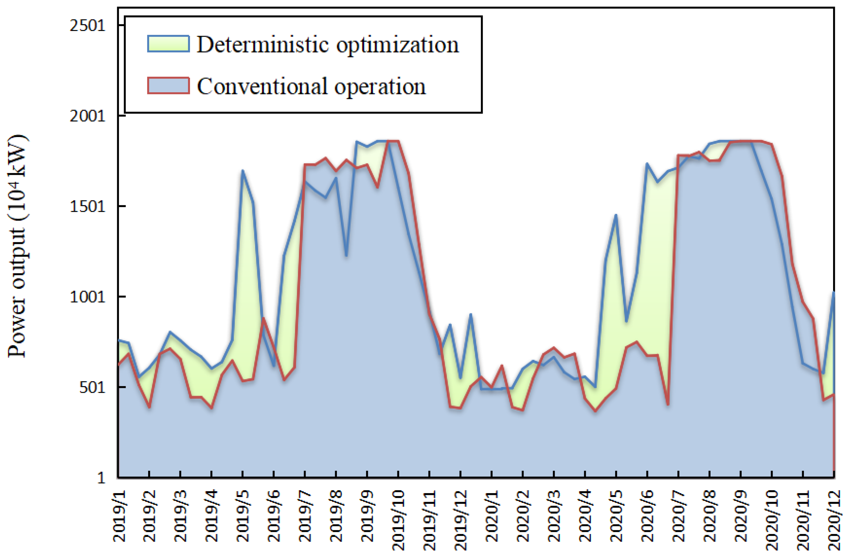
With a total length of 4504 km and a drainage area covering 1 million square kilometers, the upper Yangtze River in China has high river gradients and abundant hydropower resources [36]. As the upper Yangtze River, Jinsha River has hydropower resources that account for more than half of the whole Yangtze River basin’s output. The Xi Luo-du and Xiang Jia-ba cascade reservoirs are located at the end of Jinsha River and are important projects in the joint operation system, as shown in Figure 1. The Xi Luo-du and Xiang Jia-ba reservoirs focus on power generation, flood control, sand control and the improvement of downstream navigation. They are physically close to each other, thus they influence each other on joint scheduling [37]. The characteristic data of the Xi Luo-du and Xiang Jia-ba reservoirs are shown in

Table 1. Characteristics of the Xi Luo-du and Xiang Jia-ba reservoirs.

Reservoirs	Xi Luo-Du	Xiang Jia-Ba
Flood control water level (m)	560	370
Normal pool level (m)	600	380
Dead water level (m)	540	370
Flood storage (billion m3)	46.50	9.03
Regulating storage (billion m3)	64.60	9.03
Regulation ability	Seasonal	Seasonal
Power Capacity (MW)	12,600	6400
Firm output (MW)	3850	2009

. After collecting the data from 2014 to 2020 using a third of a month as a counting period, the first 4 years of data is used for training the models while the remaining data is used for validation. The calculated results of conventional operating and deterministic optimization are given in Figure 2, which indicates that there is an improvement promotion by using a deterministic optimization method. It can be observed that the deterministic optimization result is better, while deterministic optimization can keep water at a high level as long as possible to increase the whole operating efficiency.

5.1. Correlation Analysis in the GRA

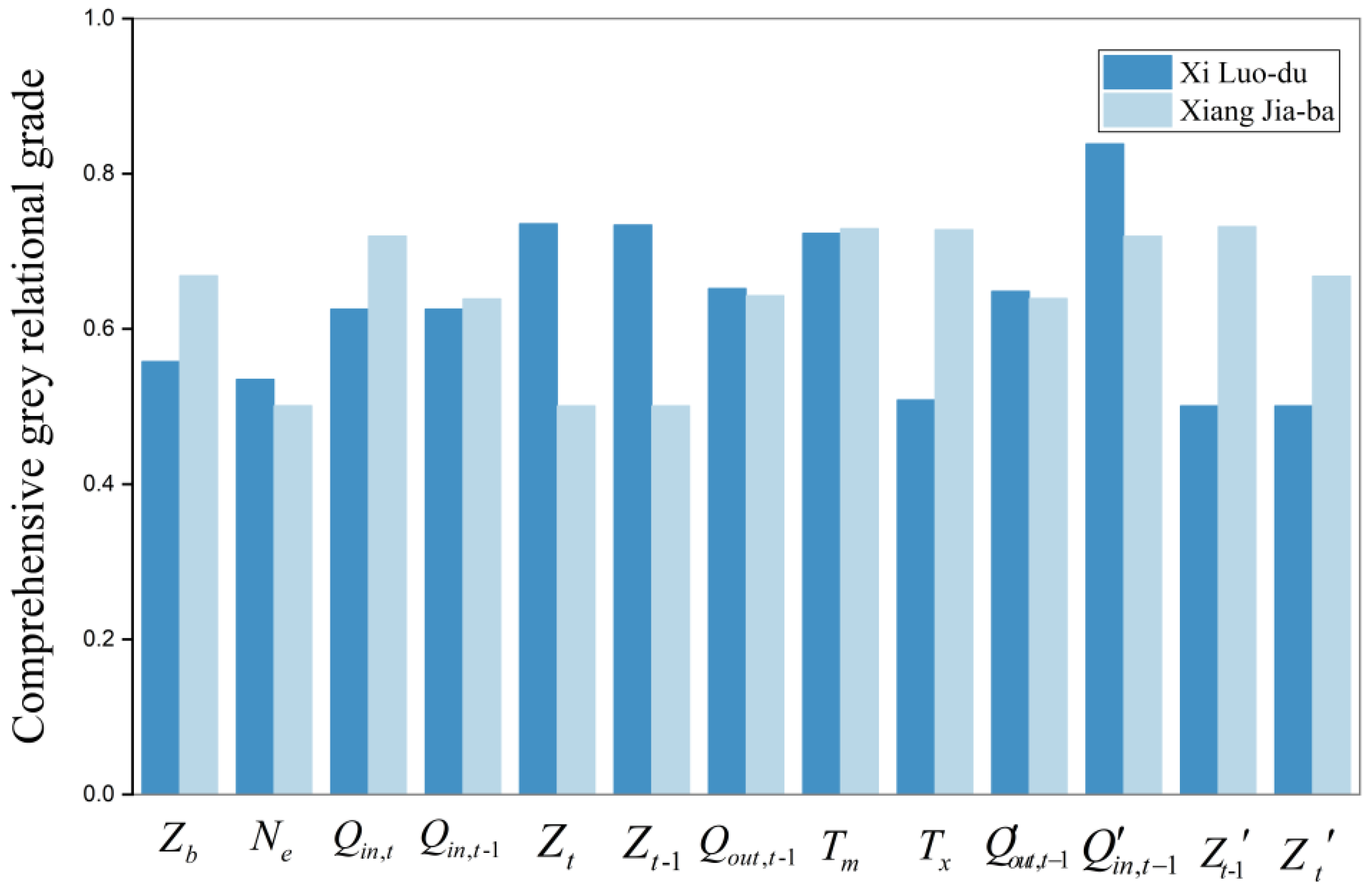
The decision variable of reservoir operation generally is chosen from among water discharge, storage capacity and power output. Due to the fact that they can be converted to each other, any one of them can be used as the decision variable and there is no difference. Compared the scheduling effect with the scheduling goal of the maximum generating capacity, this paper selects the power output as the decision variable. Specially, in order to improve the fitting efficiency of the cascade hydropower system operation rule, this paper adds relevant data of adjacent hydropower station into the input factors. Thus, the choice of correlation factor is: water level behind dam Z_b, expected output N_e, initial water level last time Z_t−1, initial water level this time Z_t, inflow last time Q_in,t−1, inflow this time Q_in,t, water discharge last time Q_out,t−1, the number of months T_m, the period number of months T_x (three periods in a month), water discharge last time in adjacent station $Q_{out,t-1}^{\prime }$, inflow last time in adjacent station $Q_{in,t-1}^{\prime }$, initial water level last time in adjacent station $Z_{t-1}^{\prime }$, and initial water level this time in adjacent station $Z_t^{\prime }$. The specific calculation results of grey relational grade are given in the

Table 2. The relational grade determined by GRA.

Reservoirs	Xi Luo-Du			Xiang Jia-Ba
Grey Relational Grade	Absolute	Relative	Comprehensive	Absolute	Relative	Comprehensive
Zb	0.61	0.50	0.56	0.83	0.50	0.67
Ne	0.57	0.50	0.53	0.50	0.50	0.50
Zt−1	0.96	0.51	0.73	0.50	0.50	0.50
Zt	0.96	0.51	0.74	0.50	0.50	0.50
Qin,t−1	0.73	0.52	0.63	0.72	0.56	0.64
Qin,t	0.73	0.52	0.63	0.77	0.66	0.72
Qout,t−1	0.79	0.51	0.65	0.78	0.51	0.64
Tm	0.94	0.51	0.72	0.96	0.50	0.73
Tx	0.52	0.50	0.51	0.96	0.50	0.73
${Q^{\prime }}_{out,t-1}$	0.78	0.51	0.65	0.77	0.51	0.64
${Q^{\prime }}_{in,t-1}$	0.78	0.89	0.84	0.77	0.66	0.72
$Z_{t-1}{}^{\prime }$	0.50	0.50	0.50	0.94	0.52	0.73
$Z_t{}^{\prime }$	0.50	0.50	0.50	0.82	0.52	0.67

. Figure 3 shows the comparison of different factors.

As shown in Table 2, the high correlation factors of the Xi Luo-du and Xiang Jia-ba reservoirs have significant differences. In the Xi Luo-du reservoir, there are four influencing factors whose comprehensive grey relational grade is above 0.7, which are initial water level last time, initial water level this time, the number of months and inflow last time in the adjacent station. In the Xiang Jia-ba reservoir, there are five influencing factors whose comprehensive grey relational grade is more than 0.7, which are inflow this time, the number of months, the period number of months, inflow last time at the adjacent station and initial water level last time at the adjacent station. Thus, the related factors of the adjacent station account for a large proportion, indicating that the data of the adjacent station also has a great contribution to the operation rule of a cascade hydropower system.

To investigate the relationship of the grey relational grade with the efficiency of operation rule derivation, this paper will divide the input vectors into three types according to the grey relational grade: (1) comprehensive grey relational grade is above 0.7 correlation factor for factors of significant correlation; (2) comprehensive grey relational grade is between 0.5 and 0.7 factor for factors of potential correlation; (3) comprehensive grey relational grade is around 0.5 for factors of no correlation. Then they are used as the input factor to make three different scheduling schemes, which fully shows the effectiveness of the proposed method in deriving reservoir operation rules and the rationality of factor selection.

5.2. Operating Rules Derivation and Results Discussion

In order to evaluate the effectiveness and rationality of the proposed method, the correlation factors were selected according to the comprehensive grey relational grades. Three schemes are proposed as follows: the first scheme adopts the significant correlation factor with the comprehensive grey relational grade above 0.7; based on the first scheme, the second scheme added potential correlation factors with comprehensive grey relational grade between 0.5 and 0.7; in the third scheme, all factors are adopted which includes factors of no correlation. The three schemes were trained and evaluated by regression analysis, and the results were revised according to the constraint conditions of output. The calculated results and regression evaluation are shown in

Table 3. The results of three schemes in regression analysis.

Reservoirs	Xi Luo-Du			Xiang Jia-Ba
Methods	GRA-SVM-1	GRA-SVM-2	GRA-SVM-3	GRA-SVM-1	GRA-SVM-2	GRA-SVM-3
R	0.918	0.961	0.953	0.990	0.994	0.992
RMSE	134.63	94.33	103.73	26.51	21.32	23.42
MAE	87.87	57.54	60.94	20.18	15.73	18.75

, while GRA-SVM-k denotes that the number of schemes is k.

As shown in Table 3, GRA-SVM-1 selects significant correlation factors for training and has already a good fitting accuracy. After adding potential correlation factor, the fitting accuracy of GRA-SVM-2 is slightly improved. Compared with GRA-SVM-1, R in GRA-SVM-2 obtains approximately 0.043 and 0.004 in two stations, respectively. However, considering that GRA-SVM-2 of the Xi Luo-du and Xiang Jia-ba reservoirs have six and five correlation factors, respectively, the enhancement of GRA-SVM-2 is not obvious. The fitting accuracy of GRA-SVM-3 is poorer than GRA-SVM-2, whose R was decreased by 0.008 and 0.002 in two stations, respectively. The results fully show that the fitting accuracy is slightly improved by adding potential correlation factors, and the increase of non-correlation factors has a negative effect.

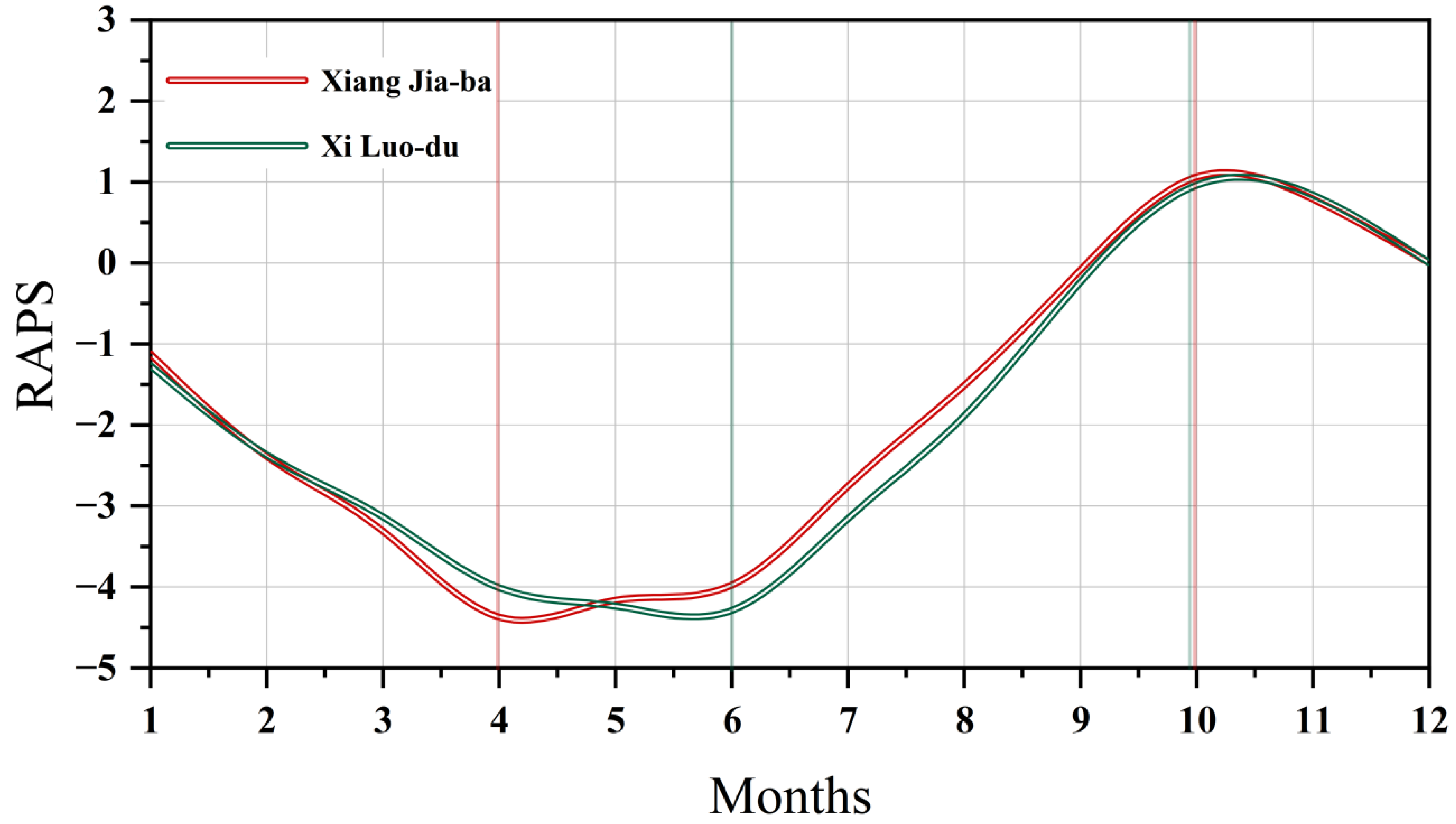
Unfortunately, small systematic changes in obtained time series are poorly visualized by statistical analysis. The RAPS analysis, based on the averaged data of GRA-SVM-2 in the Xi Luo-du and Xiang Jia-ba reservoirs, has defined three distinct periods throughout the year. Figure 4 shows the RAPS values for the average power output in the period between 2019 and 2020. The Xi Luo-du and Xiang Jia-ba reservoirs have the same visual determination of the highest “peak” in October, but not the same lowest “valley” in April and June, respectively. The difference is probably due to the different geographical positions of the two reservoirs. The sustained departure in the RAPS is the result that the average power output is continuously above-average in flood season, and continuously below-average in non-flood season. This, in fact, is the inflow changes with the season for the observed period.

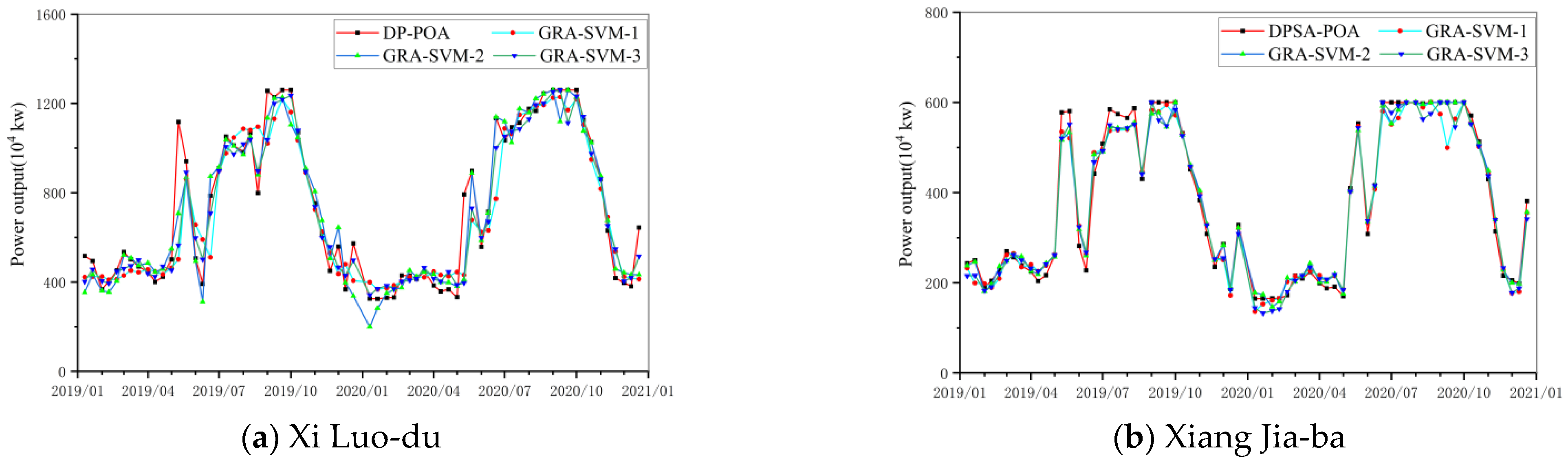
Figure 5 shows the comparison of regression evaluation in different methods. From Figure 5 and

Table 4. Comparison of operation results in different methods.

Methods	Conventional Operation	DP-POA	GRA-SVM-1		GRA-SVM-2		GRA-SVM-3
Assessment Index	Generation (108 kWh)	Generation (108 kWh)	Generation (108 kWh)	Gap (%)	Generation (108 kWh)	Gap (%)	Generation (108 kWh)	Gap (%)
Xi Luo-du	1115.46	1230.66	1183.43	3.84	1199.10	2.57	1192.19	3.13
Xiang Jia-ba	578.36	638.37	626.87	1.80	635.68	0.42	626.93	1.79

, the simulation effect is always good except the case of high output in flood season. The reason may be the situation of steep rise and fall in the flood season. Thus it is difficult to capture some of the peak values in the simulation, resulting in poor simulation effects near the peak values [25,38]. The peak value is constrained by the maximum output, which makes the simulation results closer to the deterministic optimization results but the total power generation lower. Besides, the regression evaluation results fully show that the power generation of the scheme with better regression effect is closer to the deterministic optimization results. To sum up, the GRA-SVM can provide satisfying scheduling results based on the deviated operation rule because the gap between our method and DP-POA is rather small, where the generation benefit is only 0.42% less than that produced from deterministic optimization.

6. Conclusions

In this paper, a novel operation rules derivation method based on support vector machine with grey relational analysis (GRA-SVM) is proposed for deriving the joint operation rules of cascaded hydropower reservoirs. Firstly, the GRA-SVM method uses the DP-POA methods to obtain deterministic optimization results, and then GPA is applied to quantify the influence of input vectors for making three different scheduling schemes. Two cascaded hydropower reservoirs in China (Xi Luo-du and Xiang Jia-ba) were selected as a case study, the following conclusions can be summarized as follows:

(1)

The simulation results indicate that the significant correlation factor and potential correlation factors can improve the fitting accuracy. For correlation factor, the larger the grey relational grade is, the better the fitting accuracy will be.

(2)

Among the three GRA-SVM schemes, GRA-SVM-2 has the best fitting accuracy and the absolute error of hydropower generation are 2.57 and 0.42, respectively. Therefore, in practical application, as many related factors (comprehensive grey relational grade is more than 0.5) should be selected as possible.

(3)

The GRA quantifies the importance of each correlation factor, which may as the input of the SVM model. Among the water conservancy between Xi Luo-du and Xiang Jia-ba considering the backwater effect, the relevant data of adjacent hydropower station plays an important role to improve accuracy.

References

- Feng, Z.-K.; Niu, W.-J.; Wang, W.-C.; Zhou, J.-Z.; Cheng, C.-T. A mixed integer linear programming model for unit commitment of thermal plants with peak shaving operation aspect in regional power grid lack of flexible hydropower energy. Energy 2019, 175, 618–629. [Google Scholar] [CrossRef]
- Ming, B.; Liu, P.; Guo, S.; Zhang, X.; Feng, M.; Wang, X. Optimizing utility-scale photovoltaic power generation for integration into a hydropower reservoir by incorporating long- and short-term operational decisions. Appl. Energy 2017, 204, 432–445. [Google Scholar] [CrossRef]
- Catalao, J.P.S.; Pousinho, H.M.I.; Mendes, V.M.F. Hydro energy systems management in Portugal: Profit-based evaluation of a mixed-integer nonlinear approach. Energy 2011, 36, 500–507. [Google Scholar] [CrossRef]
- Feng, Z.-K.; Niu, W.-J.; Cheng, C.-T.; Lund, J.R. Optimizing Hydropower Reservoirs Operation via an Orthogonal Progressive Optimality Algorithm. J. Water Resour. Plan. Manag. 2018, 144, 04018001. [Google Scholar] [CrossRef]
- Chang, J.-X.; Bai, T.; Huang, Q.; Yang, D.-W. Optimization of Water Resources Utilization by PSO-GA. Water Resour. Manag. 2013, 27, 3525–3540. [Google Scholar] [CrossRef]
- Yu, Y.; Wang, P.-F.; Wang, C.; Qian, J.; Hou, J. Combined Monthly Inflow Forecasting and Multiobjective Ecological Reservoir Operations Model: Case Study of the Three Gorges Reservoir. J. Water Resour. Plan. Manag. 2017, 143, 05017004. [Google Scholar] [CrossRef]
- Zhao, T.; Cai, X.; Lei, X.; Wang, H. Improved Dynamic Programming for Reservoir Operation Optimization with a Concave Objective Function. J. Water Resour. Plan. Manag. ASCE 2012, 138, 590–596. [Google Scholar] [CrossRef]
- Philbrick, C.R.; Kitanidis, P.K. Limitations of deterministic optimization applied to reservoir operations. J. Water Resour. Plan. Manag. 1999, 125, 135–142. [Google Scholar] [CrossRef]
- Madani, K. Hydropower licensing and climate change: Insights from cooperative game theory. Adv. Water Resour. 2011, 34, 174–183. [Google Scholar] [CrossRef]
- Wu, C.L.; Chau, K.W. Prediction of rainfall time series using modular soft computing methods. Eng. Appl. Artif. Intell. 2013, 26, 997–1007. [Google Scholar] [CrossRef] [Green Version]
- Young, G.K. Finding reservoir operating rules. J. Hydraul. Div. 1967, 93, 297–321. [Google Scholar] [CrossRef]
- Ji, C.; Su, X.; Zhou, T. Study on the optimal operating rules for cascade hydropower stations based on output allocation model. J. Hydroelectr. Eng. 2010, 30, 26–31. [Google Scholar]
- Yang, P.; Ng, T.L. Fuzzy Inference System for Robust Rule-Based Reservoir Operation under Nonstationary Inflows. J. Water Resour. Plan. Manag. 2017, 143, 04016084. [Google Scholar] [CrossRef]
- Bozorg-Haddad, O.; Aboutalebi, M.; Ashofteh, P.-S.; Loaiciga, H.A. Real-time reservoir operation using data mining techniques. Environ. Monit. Assess. 2018, 190, 594. [Google Scholar] [CrossRef]
- Chau, K.W. Particle swarm optimization training algorithm for ANNs in stage prediction of Shing Mun River. J. Hydrol. 2006, 329, 363–367. [Google Scholar] [CrossRef] [Green Version]
- Wang, W.-C.; Xu, D.-M.; Chau, K.-W.; Chen, S.-Y. Improved annual rainfall-runoff forecasting using PSO-SVM model based on EEMD. J. Hydroinform. 2013, 15, 1377–1390. [Google Scholar] [CrossRef]
- Hsu, C.W.; Lin, C.J. A simple decomposition method for support vector machines. Mach. Learn. 2002, 46, 291–314. [Google Scholar] [CrossRef] [Green Version]
- Cheng, C.-T.; Feng, Z.-K.; Niu, W.-J.; Liao, S.-L. Heuristic Methods for Reservoir Monthly Inflow Forecasting: A Case Study of Xinfengjiang Reservoir in Pearl River, China. Water 2015, 7, 4477–4495. [Google Scholar] [CrossRef]
- Ullah, K.; Garg, H.; Mahmood, T.; Jan, N.; Ali, Z. Correlation coefficients for T-spherical fuzzy sets and their applications in clustering and multi-attribute decision making. Soft Comput. 2020, 24, 1647–1659. [Google Scholar] [CrossRef]
- Zhu, Y.; Tian, D.; Yan, F. Effectiveness of Entropy Weight Method in Decision-Making. Math. Probl. Eng. 2020, 2020, 3564835. [Google Scholar] [CrossRef]
- Chan, J.W.K.; Tong, T.K.L. Multi-criteria material selections and end-of-life product strategy: Grey relational analysis approach. Mater. Des. 2007, 28, 1539–1546. [Google Scholar] [CrossRef]
- Kuo, Y.-Y.; Yang, T.-H.; Huang, G.-W. The use of grey relational analysis in solving multiple attribute decision-making problems. Comput. Ind. Eng. 2008, 55, 80–93. [Google Scholar] [CrossRef]
- Tosun, N. Determination of optimum parameters for multi-performance characteristics in drilling by using grey relational analysis. Int. J. Adv. Manuf. Technol. 2006, 28, 450–455. [Google Scholar] [CrossRef]
- Wei, G.-W. Gray relational analysis method for intuitionistic fuzzy multiple attribute decision making. Expert Syst. Appl. 2011, 38, 11671–11677. [Google Scholar] [CrossRef]
- Feng, Z.-K.; Niu, W.-J.; Cheng, X.; Wang, J.-Y.; Wang, S.; Song, Z.-G. An effective three-stage hybrid optimization method for source-network-load power generation of cascade hydropower reservoirs serving multiple interconnected power grids. J. Clean. Prod. 2020, 246, 119035. [Google Scholar] [CrossRef]
- Feng, Z.-K.; Niu, W.-J.; Wang, S.; Cheng, C.-T.; Jiang, Z.-Q.; Qin, H.; Liu, Y. Developing a successive linear programming model for head-sensitive hydropower system operation considering power shortage aspect. Energy 2018, 155, 252–261. [Google Scholar] [CrossRef]
- Niu, W.-J.; Feng, Z.-K.; Feng, B.-F.; Min, Y.-W.; Cheng, C.-T.; Zhou, J.-Z. Comparison of Multiple Linear Regression, Artificial Neural Network, Extreme Learning Machine, and Support Vector Machine in Deriving Operation Rule of Hydropower Reservoir. Water 2019, 11, 88. [Google Scholar] [CrossRef] [Green Version]
- Pan, Z.; Chen, L.; Teng, X. Research on joint flood control operation rule of parallel reservoir group based on aggregation-decomposition method. J. Hydrol. 2020, 590, 125479. [Google Scholar] [CrossRef]
- Dong, S. Multi class SVM algorithm with active learning for network traffic classification. Expert Syst. Appl. 2021, 176, 114885. [Google Scholar] [CrossRef]
- Geng, D.; Alkhachroum, A.; Melo Bicchi, M.A.; Jagid, J.R.; Cajigas, I.; Chen, Z.S. Deep learning for robust detection of interictal epileptiform discharges. J. Neural Eng. 2021, 18, 056015. [Google Scholar] [CrossRef] [PubMed]
- Deng, J. Control problems of grey systems. Syst. Control Lett. 1982, 1, 288–294. [Google Scholar]
- Garbrecht, J.; Fernandez, G.P. Visualization of trends and fluctuations in climatic records. J. Am. Water Resour. Assoc. 1994, 30, 297–306. [Google Scholar] [CrossRef]
- Bonacci, O.; Bonacci, D.; Roje-Bonacci, T. Different air temperature changes in continental and Mediterranean regions: A case study from two Croatian stations. Theor. Appl. Climatol. 2021, 145, 1333–1346. [Google Scholar] [CrossRef]
- Sajid, T.; Tanveer, S.; Sabir, Z.; Guirao, J.L.G. Impact of Activation Energy and Temperature-Dependent Heat Source/Sink on Maxwell-Sutterby Fluid. Math. Probl. Eng. 2020, 2020, 5251804. [Google Scholar]
- Markovinovic, D.; Kranjcic, N.; Durin, B.; Orsulic, O.B. Identifying the Dynamics of the Sea-Level Fluctuations in Croatia Using the RAPS Method. Symmetry 2021, 13, 289. [Google Scholar] [CrossRef]
- Qiu, H.; Chen, L.; Zhou, J.; He, Z.; Zhang, H. Risk analysis of water supply-hydropower generation-environment nexus in the cascade reservoir operation. J. Clean. Prod. 2021, 283, 124239. [Google Scholar] [CrossRef]
- Wang, Q.; Zhou, J.; Dai, L.; Huang, K.; Zha, G. Risk assessment of multireservoir joint flood control system under multiple uncertainties. J. Flood Risk Manag. 2021, e12740. [Google Scholar] [CrossRef]
- Wu, Y.; Fang, H.; Huang, L.; Ouyang, W. Changing runoff due to temperature and precipitation variations in the dammed Jinsha River. J. Hydrol. 2020, 582, 124500. [Google Scholar] [CrossRef]
Figure 1.
Location of the cascade reservoirs including the Xi Luo-du Reservoir and Xiang Jia-ba reservoir in the upper Yangtze River.
Figure 2.
Comparation of output process between conventional operating and deterministic optimization results.
Figure 3.
Grey relational grade between different correlation factors and decision variable.
Figure 4.
PAPS of obtained time series of power output.
Figure 5.
Comparison between deterministic optimization and three GRA-SVM schemes.