
A Comparison of In-Sample and Out-of-Sample Model Selection Approaches for Artificial Neural Network (ANN) Daily Streamflow Simulation

1
Department of Water Management & Hydrological Science, Texas A&M University, College Station, TX 77843, USA
2
Department of Biological & Agricultural Engineering, Texas A&M University, College Station, TX 77843, USA
*
Author to whom correspondence should be addressed.
Water 2021, 13(18), 2525; https://doi.org/10.3390/w13182525
Submission received: 5 August 2021
/
Revised: 6 September 2021
/
Accepted: 11 September 2021
/
Published: 15 September 2021
(This article belongs to the Section Hydrology)
Abstract
:Artificial Neural Networks (ANN) have been widely applied in hydrologic and water quality (H/WQ) modeling in the past three decades. Many studies have demonstrated an ANN’s capability to successfully estimate daily streamflow from meteorological data on the watershed level. One major challenge of ANN streamflow modeling is finding the optimal network structure with good generalization capability while ameliorating model overfitting. This study empirically examines two types of model selection approaches for simulating streamflow time series: the out-of-sample approach using blocked cross-validation (BlockedCV) and an in-sample approach that is based on Akaike’s information criterion (AIC) and Bayesian information criterion (BIC). A three-layer feed-forward neural network using a back-propagation algorithm is utilized to create the streamflow models in this study. The rainfall–streamflow relationship of two adjacent, small watersheds in the San Antonio region in south-central Texas are modeled on a daily time scale. The model selection results of the two approaches are compared, and some commonly used performance measures (PMs) are generated on the stand-alone testing datasets to evaluate the models selected by the two approaches. This study finds that, in general, the out-of-sample and in-sample approaches do not converge to the same model selection results, with AIC and BIC selecting simpler models than BlockedCV. The ANNs were found to have good performance in both study watersheds, with BlockedCV selected models having a Nash–Sutcliffe coefficient of efficiency (NSE) of 0.581 and 0.658, and AIC/BIC selected models having a poorer NSE of 0.574 and 0.310, for the two study watersheds. Overall, out-of-sample BlockedCV selected models with better predictive ability and is preferable to model streamflow time series.
1. Introduction
The estimation of streamflow time series on the watershed scale is of great importance in surface water hydrology. Accurate streamflow is the foundation of water resources planning and management, including river hydraulics modeling and engineering project design, water demand assessment and allocation, and water quality studies [1,2]. Data-driven methods have gained popularity in hydrologic and water quality (H/WQ) modeling in recent years due to their effectiveness in mapping connections between hydrologic inputs and outputs [3]. Among these methods, the artificial neural network (ANN) has proven to be an effective tool in water resources modeling [4,5].
An ANN is a “parallel-distributed processor” that resembles the biological neural network structure of the human brain. The ANN acquires knowledge or information from a learning process and stores that knowledge in interneuron links using a weighted matrix. The early concept of ANNs as a computational tool was formalized in the 1940s. It went through gradual development in the ensuing decades as computers become more accessible and computational efficiency grew [6]. ANN-based models hold some clear advantages over conventional conceptual models in H/WQ modeling. ANNs do not require a priori knowledge of the physical characteristics of the study watershed as model input, thus significantly reducing the procedures for model setup and simulation [7,8]. When sufficient data have been provided, ANN models have produced satisfactory results for streamflow forecasting, according to a review provided by Yaseen et al. [9]. However, some believe modeling hydrologic systems with ANNs without explaining the underlying physical processes is a significant drawback. For instance, the lack of capability to capture physical dynamics at the watershed level means that ANNs are not suitable for modeling streamflow under changing climate or land use conditions. In addition, the ANN’s predictive capability is often unreliable beyond the training data range due to the absence of physical explanation [9,10,11,12,13]. Worland et al. [3] further recommended that machine-learning models such as ANNs only be used for making predictions rather than gaining hydrological insights.
ANN application in hydrology began in the 1990s. Since then, many studies have applied ANNs in H/WQ modeling. Several studies have reported satisfactory results using ANNs for streamflow estimation. Karunanithi et al. [13] demonstrated successful streamflow prediction at the Huron River in Michigan using neural network models in an early study. The predicted flow closely matched the timing and magnitude of the actual flow. Ahmed and Sarma [14] used three data-driven models to generate synthetic streamflow for the Pagladia River in northeast India and concluded that the ANN-based model has the best performance. Birikundavyi et al. [15] compared an ANN to an autoregressive model to forecast daily streamflow in the Mistassibi River in northeastern Quebec. They obtained results showing that the ANN model outperformed the autoregressive model. Similarly, Hu et al. [16] showed an ANN-based model that simulated daily streamflow and annual reservoir inflow for two watersheds in northern China that outperformed an auto-regressive model. Humphrey et al. [5] coupled an ANN model and a conceptual rainfall–runoff model to produce a monthly streamflow forecast for a drainage network in southeast Australia. They reported that the hybrid model outperformed the original conceptual model, especially for high flow periods. Isik et al. [17] reported that accurate daily streamflow prediction was achieved using a hybrid model based on an ANN and the SCS (Soil Conservation Service, the US Department of Agriculture) curve number method. Kişi [18] compared four different ANN algorithms for streamflow forecasting, all of which reached satisfactory statistical results with correlation coefficients of all four models close to one. Rezaeianzadeh et al. [19] simulated daily watershed outflow at the Khosrow Shirin watershed in Iran, using an ANN and HEC-HMS, and concluded that the ANN model with a multi-layer perceptron was more efficient in forecasting daily streamflow.
Although the literature has demonstrated that ANN models can make satisfactory streamflow predictions, the ANN-based models often suffer from overfitting problems due to a relatively large number of parameters to be estimated compared with other statistical-based models [20]. Model overfitting often refers to ANNs fitting the in-sample data (training set) well but the out-of-sample data (testing set) poorly. Selecting the appropriate model structure is crucial for accurately simulating streamflow while ameliorating overfitting. Routinely, several ANN models are trained, and a model selection phase is applied to find the model with the best generalization capability [21]. Two main types of model selection approaches are often adopted for this purpose. The out-of-sample approach, based on cross-validation, divides the available data into training, validation, and testing sets. The in-sample approach relies on in-sample criterion calculated on the training dataset, most notably Akaike’s information criterion (AIC) and Bayesian information criterion (BIC), for deciding the models’ generalization capability [22]. Although it is generally accepted that the performance of statistical models should be assessed using out-of-sample tests rather than in-sample errors [23], the in-sample model selection approach has the clear advantage of utilizing all available data for modeling training while avoiding data splitting. Previous studies have discussed the benefits and disadvantages of the two approaches. Arlot and Celisse [24] argued that out-of-sample cross-validation is more applicable in many practical situations. Qi and Zhang [22] showed that the results of a few in-sample model selection criteria were not consistent with the out-of-sample performance for three economic time series. On the other hand, a study conducted by Shao [25] concluded that AIC and leave-one-out cross-validation (LOOCV) converge to the same model selection result. It is unclear how the out-of-sample and in-sample model selection approaches will perform on hydrological time series without actual experimentation. Additionally, as noted by Bergmeir and Benítez [26], the distinct nature of different time series can cause a model selection method to work well with a particular type of time series but show poor performance on others. Hence, it is yet to be evaluated if the model selection outcomes of these two approaches converge for a hydrological time series.
The main objectives of this study are: (1) to create ANN rainfall–streamflow models on the watershed level, (2) determine the optimal model structure of the ANNs using both in-sample and out-of-sample model selection approaches, (3) compare the model selection results of these two approaches, and (4) empirically investigate their efficacy in selecting the optimal neural network. The task is to be accomplished using two small watersheds in the San Antonio region of south-central Texas, one of which is dominated by a well-developed urban landscape. An agricultural landscape primarily covers the other. The streamflow simulations are to be conducted on a daily time step for the outflows of both watersheds. The following sections will describe the details of the models.
2. Materials and Methods
2.1. Study Area and Data Acquisition
The city of San Antonio is in the sub-tropic and semi-humid climate zone of south-central Texas. It has long hot summers and warm to cool winters. Snowfall has been reported historically, although it is rare. The San Antonio region is about 210 m above sea level and has an annual precipitation of around 770 mm [27]. Combining the rapidly growing total population and a decline of population density at its urban center, San Antonio is one of the fastest-growing metropolitan areas in the US [28,29].
This study selected two adjacent small watersheds in the San Antonio region for streamflow modeling (Figure 1). The headwaters of the San Antonio River Basin (HSARB, HUC10: 1210030102) are centered at 98.507° west longitude, 29.422° north latitude, and mainly cover the extent of central downtown San Antonio. HSARB has a drainage area of 395.84 km2, of which 81.66% is classified as developed urban area according to the 2011 National Land Cover Database (NLCD2011) land use land cover (LULC) classification [30]. The main waterway in the HSARB is the San Antonio River, which originates in the metropolitan area of San Antonio, flows southeast across downtown San Antonio and merges with the Medina River in the city’s southern suburbs. Thus, the most downstream point of the drainage basin is located at the southern tip of the HSARB. The streamflow close to the watershed outlet is measured by a USGS surface streamflow gauge (USGS 08178565). The Lower Medina River Basin (LMRB), centered at 98.698° west longitude, 29.319° north latitude, is located west of the San Antonio urban area and shares a short watershed boundary with HSARB. LMRB has a drainage area of 929.29 km2 and is much less developed in comparison to the HSARB. The dominant land cover types at LMRB are shrub, pasture, and cultivated crop, covering 25.97%, 15.72%, and 14.38% of the entire LMRB, respectively. The major waterway in LMRB is the Medina River, which flows southeast and merges into the San Antonio River at the outlet of LMRB. The streamflow measurement station closest to the watershed outlet is USGS gauge 08181500, which covers most of the drainage area of the LMRB, located about 7 km from the watershed outlet. The proximity in geographic locations of the two study watersheds helps to reduce uncertainties that may arise in model comparison, as the neighboring watersheds have similar climatology, geology, and hydrology.
Meteorological and hydrological data of the two watersheds were used to train the neural network models. The Parameter-elevation Regressions on Independent Slopes Model (PRISM) daily spatial climate dataset AN81d, produced by the PRISM Climate Group at Oregon State University [31], was used for meteorological inputs in this study. PRISM data are accessed using the Google Earth Engine (GEE), a cloud-based geospatial analysis platform that provides access to freely available geospatial data archives produced by multiple government agencies [32]. Polygon masks that cover each watershed are uploaded to the GEE server. The area-averaged daily precipitation and mean temperature are calculated and separately obtained for the two masked areas. The daily discharge observations for the gauges closest to the watershed outlets and their corresponding upstream gauges are obtained from the USGS surface water daily measurement [33].
2.2. ANN Model Description
The purpose of applying an ANN as a rainfall–streamflow model is to create a specific model structure that can capture the nonlinear relationships between the input precipitation and target streamflow. A multi-layer feed-forward neural network normally has one input layer, one output layer, and at least one hidden layer that connects the input and output layers. A three-layer feed-forward neural network using a back-propagation algorithm is often employed in hydrological modeling and is generally sufficient for streamflow and water quality simulations [8,10,34]. Each layer possesses at least one node (or neuron) for a standard three-layer feed-forward neural network, and each node is connected to all other nodes in its adjacent layers. The connection links between nodes contain associated weights and biases that represent their connection strength. At each node, a nonlinear transformation, often referred to as a transfer function, is applied to the net input of the node to calculate its corresponding output signal. The weights and biases are randomly initialized before training begins and updated using the back-propagation step in every training epoch [10]. The operation at a node can be defined using Equation (1),
where is the node’s output signal, is the transfer function, represents the weight vectors associated with the interneuron links, is the input vector, and is the bias [10].
ANN models use the back-propagation algorithm to update the weight and bias terms described in Equation (1). The back-propagation algorithm is one of the most popular algorithms for ANN training [10,35]. Back-propagation minimizes the network loss function, which is usually in the squared error form as described in Equation (2), using the gradient descent method [10],
where is the observation, is the corresponding ANN prediction, is the number of observations, and is the number of output nodes.
The loss computed from Equation (2) is propagated backward through the network to each node, and the weights are updated along the steepest descent of the loss function in every training epoch. The weight change of an epoch can be described with Equation (3) [10],
where and are weight increments between node and during the th and th epoch, is the loss function computed using Equation (2), and and are learning rate and momentum constant [10].
2.3. Model Selection Approaches
2.3.1. Blocked Cross-Validation
Traditionally, the out-of-sample model selection approach is more often used on ANN models [23]. Cross-validation is the simplest and most widely used method for estimating prediction error, according to Hastie et al. [36]. It directly uses the out-of-sample error for model selection. In H/WQ modeling, the cross-validation-based approach was applied in several previous studies [5,7,37,38,39,40,41]. The model cross-validation procedure splits the available data into three groups: training, validation, and testing. The training set is used for model training, during which the free parameters (i.e., interneuron weights and biases) are estimated for several ANN models with specific model structures. Following the training set, the prediction performance for the models is calculated on the hold-out validation set, and the model that has the best validation performance is selected. The testing set is an independent dataset used for stand-alone measurement of model generalization capability [10,13]. Nevertheless, Bergmeir and Benítez [26] stated that time series data are intrinsically ordered. Therefore, its time dependency and autocorrelation contradict the basic assumption of traditional cross-validation that the data are independent and identically distributed (i.i.d.). The authors have further suggested using blocks of data rather than resampling data randomly in each cross-validation iteration to avoid breaking the data dependency of the studied time series.
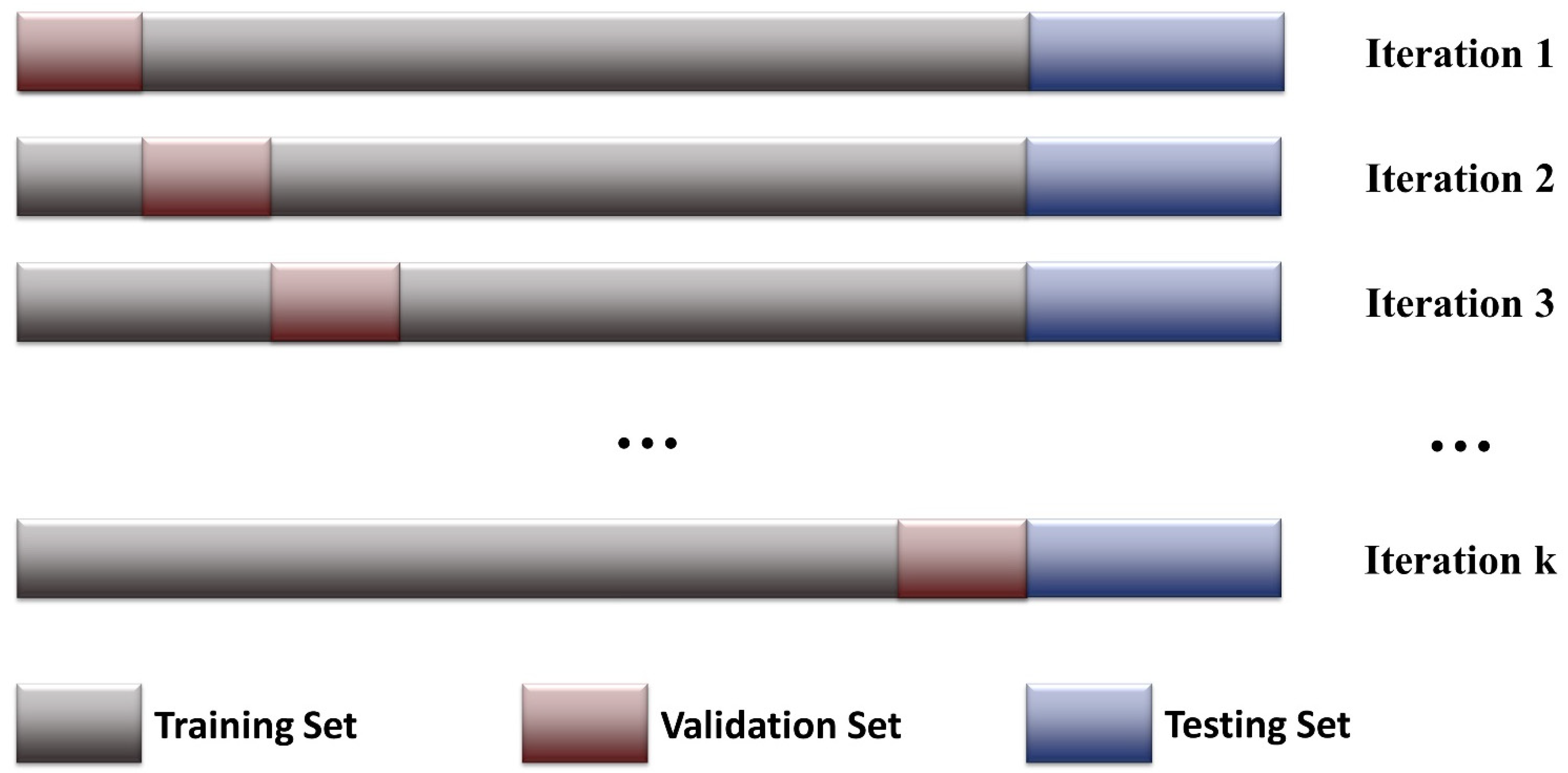
To address the issue that the streamflow time series usually has strong autocorrelation, this study applies blocked cross-validation (BlockedCV) as the out-of-sample model selection approach to be evaluated. Unlike the normal k-fold cross-validation that randomly samples training and validation data, the training/validation data split in BlockedCV maintains the data points’ sequential order by grouping them into several data blocks, and all data blocks are fixed throughout the cross-validation process (Figure 2).
Although the out-of-sample test performance is more often accepted as reliable for model selection, some of its limitations are noted in the literature. For example, James et al. [42] summarized from past studies that data splitting might significantly increase the variability of the estimates. As the partition of available data is usually carried out subjectively by the modelers, the performance results can be intensely dependent on where the data splitting takes place between training and validation sets and hence influence the outcome of the selected best model. Moreover, since statistical methods tend to perform better when trained with larger datasets, omitting part of the available data for model validation may compromise model training, especially when the size of the available dataset is small [26].
2.3.2. AIC and BIC
The in-sample model selection approach is based on the in-sample criterion calculated for the training dataset, which avoids data splitting and enables utilizing all available data for model training. This approach usually considers the in-sample estimation error and model complexity together in its various forms of equations. The size of estimated parameters is often added into the equations as a penalty term since a more complex model is more likely to cause model overfitting. Akaike’s information criterion (AIC) and the Bayesian information criterion (BIC) are two of the most widely used in-sample model selection criteria [22]. AIC and BIC are founded on information theory and are motivated by the need for balancing goodness-of-fit and model complexity [43]. Lower AIC and BIC values indicate a better model fit. Various forms of AIC and BIC can be found in the literature. This study uses the form proposed by Qi and Zhang [22]. One common form of AIC [44] is given in Equation (4):
where is the number of model parameters, and is the number of observations. is the maximum likelihood estimate of the variance of the residual term, expressed by Equation (5):
where is the observation, and is the model estimate at time .
BIC has a common format that resembles AIC. Although, it imposes a greater penalty for model complexity, which tends to give preference to simpler models [36]. BIC can be defined by Equation (6) as:
For linear models for which AIC and BIC were originally designed, represents the number of estimated parameters. For nonlinear and other complex models, is usually replaced by some measure of model complexity [36]. In a three-layer neural network model, the two critical uncertainties associated with the model structure are the number of the input vectors () and the number of hidden layer units (). Qi and Zhang [22] have proposed using to measure the model complexity of a three-layer feed-forward neural network, which this study adopts. One big limitation of the in-sample model selection approach is that the in-sample errors are likely to underestimate forecasting errors. Thus, using the best in-sample fit, the model selected may not make the best prediction of unseen time series [23].
2.4. Model Performance Measures
The performance of the models on the partitioned datasets is evaluated using three goodness-of-fit measures: the Nash–Sutcliffe coefficient of efficiency (NSE), percent bias (PBIAS), and root mean square error to observation standard deviation ratio (RSR). The NSE is a dimensionless index mainly used in H/WQ modeling; it is a normalized statistic determining the magnitude of residual variance compared to observed data variance [45]. The NSE is expressed in Equation (7) as:
where is the variable, obs and sim stand for observed and simulated, respectively. NSE ranges from −∞ to 1.0, with NSE = 1.0 representing the optimal fitting. A negative NSE value indicates that the mean observed value is a better fit than the simulated value [46,47,48].
The PBIAS measures the average tendency of simulated data to be larger or smaller than the observations. The model reaches optimal prediction with a PBIAS of 0.0, and smaller absolute PBIAS indicates a more accurate model prediction. In the following form, positive PBIAS values indicate that the model output overestimates the observation, while negative values indicate underestimation [48]. PBIAS is defined in Equation (8) as:
The RSR standardizes the root mean square error (RMSE) by dividing it by the standard observation deviation, which facilitates convenient performance evaluation. The RSR is a dimensionless index that ranges from 0 to a substantially large positive value, with the optimal value 0 indicating 0 residual variations and, therefore, perfect model fit [48]. The RSR is defined as:
Moriasi et al. [48] proposed performance evaluation criteria (PEC) corresponding to the above performance measures on a monthly time step. Since H/WQ models perform better at coarser time scales, Kalin et al. [49] developed relaxed performance qualitative ratings on NSE and PBIAS for finer time step models. This study simulates the streamflow on a daily time scale and adopts the performance evaluation criteria from several previous studies [48,49,50,51]. The PEC used in this study are summarized in Table 1.
2.5. ANN Models Setup
Determining the best input variable combinations is essential for successfully training an ANN model [52]. Previous research on ANN streamflow forecasting has mainly applied meteorological variables and discharge from the preceding time steps as model inputs [7,8,19,35,53,54]. This study proposes using the discharge measurements from an upstream gauge and meteorological variables as inputs for the ANN models. The proposed input combinations are summarized in Table 2. These five model prediction scenarios were applied to both study watersheds. The selected variables include daily precipitation (Pt), precipitation of the previous n days (Pt−n), daily mean air temperature (Tt), streamflow measurement from the upstream gauge stations (Qu, USGS 08178000, USGS 08180700), and total precipitation for the preceding n days (Pn). Precipitation and temperature were selected as inputs mainly because they are the most relevant meteorological variables for hydrological impact studies [55]. In addition, the total precipitation of previous time steps is included to represent the antecedent moisture condition in scenarios 4 and 5. The downstream discharge (Q, USGS 08178565, USGS 08181500) close to the watershed outlets are the training targets. The input combinations proposed here avoid using the streamflow of preceding time steps at the estimated site, which allows for application of the modeling approach in regions where streamflow observations are incomplete.
Input and output data for setting up the ANN models were obtained from the PRISM database and USGS publicly accessible data. While the PRISM daily spatial climate dataset has complete temporal coverage for the years starting from 1981, the USGS streamflow observations often have long durations of missing data. This study uses a decade-long daily time series for model input and output, the longest available consistent data for the two study watersheds. Simulations for the HSARB were run from 1 October 1987 to 30 September 1997, and for the LMRB, from 1 October 1997 to 30 September 2007. The first 70% of data are used for model training (in-sample approach) or training/validation (out-of-sample approach), and the remaining 30% of data are used as the stand-alone testing set.
The Cox and Stuart test [56] was applied to detect whether the precipitation and observed streamflow time series during the study period had a time-dependent trend. The decade-long time series of precipitation, upstream discharge, and target discharge were divided into thirds. The test compared whether the first third of the data was larger or smaller than the last third. As the last third of the time series covered the entire testing period, this test can be used to assess if the testing period data trended away from the training period.
The Cox and Stuart test results showed that in HSARB, the precipitation, upstream discharge, and target discharge all had extremely small p-values, approximately 0, which indicated a detectable trend in the 10-year time series. Hence, differences between the training and testing data exist in HSARB. Meanwhile, in LMRB, the precipitation data had a p-value close to 0, while the upstream discharge had a p-value of 0.939 and target discharge had a p-value of 0.028, which showed that if the p-value threshold of 1% is applied, the test failed to reject the null hypothesis that no monotonic trend exists in the discharge time series. This result suggested no significant difference between the training and testing discharge data in LMRB, while the precipitation pattern had altered during the study period. The more fluctuating discharge data in HSARB could cause relatively poor predictive outcomes in the testing period, while the stable discharge condition in LMRB is likely to induce better predictive performance in the testing period.
This study applied a three-layer feed-forward neural network with input/output layers and a single hidden layer. The logistic function is used as the transfer function for all hidden nodes, and the popular back-propagation algorithm is used to train the models. The maximum amount of training epoch was set as 200,000 to ensure training coverages, while the learning rate was set as 0.002. In addition to different configurations of input variables, the size of hidden layer units significantly affects the complexity of a neural network and its predictive capability. Unfortunately, there is no unified theory in the literature to determine the optimum number of hidden units [10]. In this study, the number of hidden units is varied from 1 to 10. Larger hidden layer sizes are excluded from the experimentation, since models with larger hidden layer sizes tend to overfit the training data [39].
Because hydrologic variables span different magnitudes, prior to their use in neural networks, they should be normalized to a common scale to aid in comparison [57,58]. In this study, the input and output variables are normalized on the range of 0 to 1 using the following equation:
where , , and denote the observed, minimum, and maximum values of the raw data, respectively, and denotes the normalized values. R software (R Foundation for Statistical Computing: Vienna, Austria) [59] was used for data processing and model simulations. The “neuralnet” package was used for training all the ANNs in this work.
3. Results and Discussion
The in and out of sample model selection approaches discussed in Section 2.3 were used to determine the best input combination and the optimum number of hidden layer units of each model scenario in Table 2. Therefore, two groups of models were created for every scenario, one for each approach. The first group of models applies the in-sample model selection criteria (AIC and BIC), splitting the data between training and testing sets as indicated earlier. The BlockedCV is applied to the second group of model scenarios. The first 70% of available data were partitioned into ten fixed blocks; then, ten training iterations were run using a loop structure with 1/10 of the data serving as the validation set in each iteration. The NSE calculated on the validation sets from all iterations is averaged to obtain the validation statistics used as the selection criterion of the BlockedCV. Moreover, all three performance measures discussed in Section 2.4 are calculated for the training, validation, and testing datasets to further evaluate the model generalization capability and compare the performance among different ANN models.
3.1. Optimum Hidden Layer Size Selection
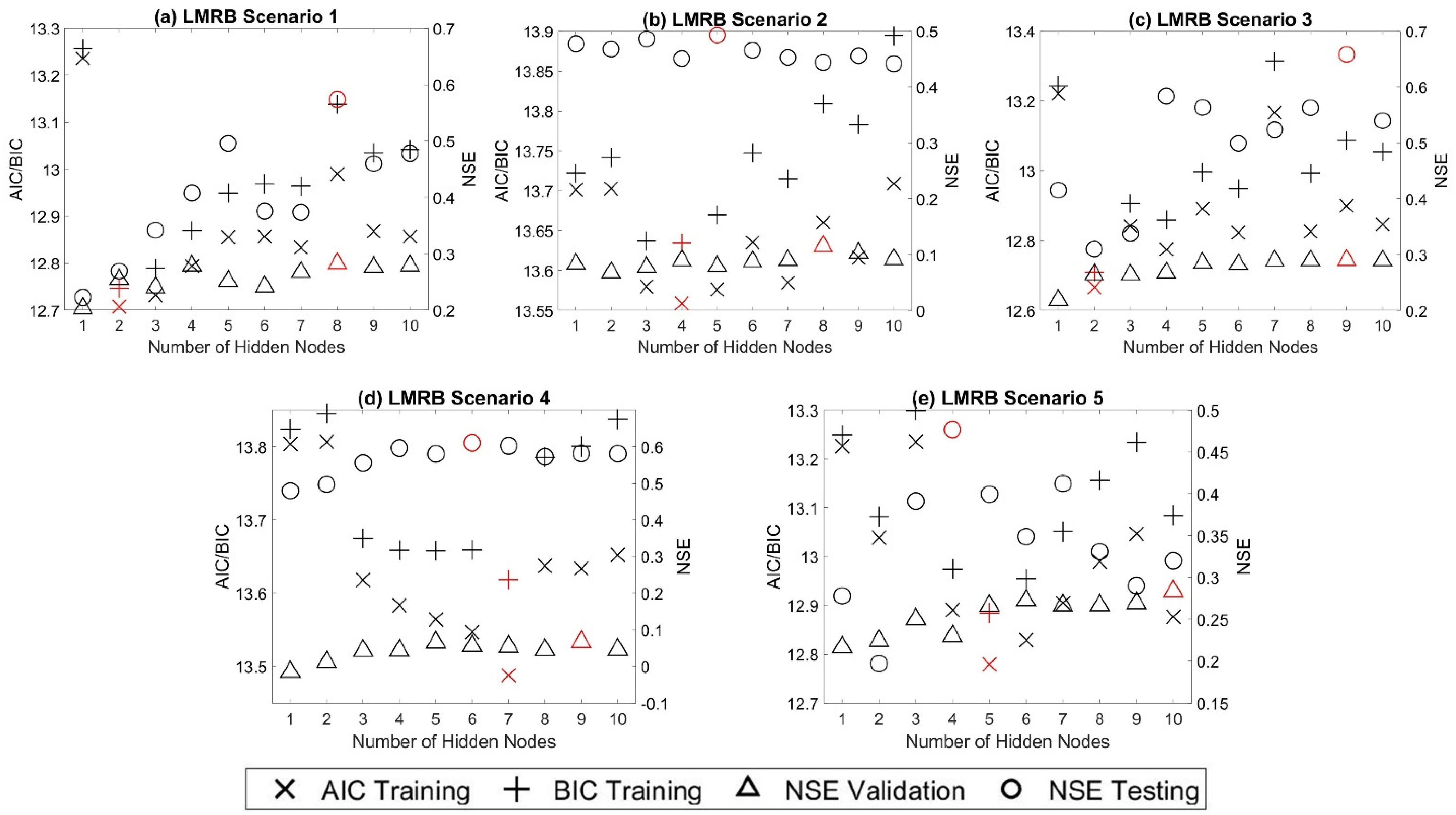
The AIC and BIC of the training dataset for the in-sample modeling group, the NSE of the validation dataset for the out-of-sample modeling group, and the NSE calculated on the stand-alone testing dataset are displayed in Figure 3 for the HSARB and Figure 4 for the LMRB. In Figure 3 and Figure 4, the AIC and BIC are measured using the left axis, while the NSE is measured using the right axis. From plots a−e of these two figures, no uniform trends are observed for the performance measures as the number of hidden nodes increases across the five prediction scenarios for both watersheds. The best performance measures of each scenario (i.e., the smallest AIC and BIC, the largest NSE) are highlighted in red. Among all ten prediction scenarios for the two watersheds, in seven out of ten scenarios the best AIC and BIC resulted from the same number of nodes in the hidden layer. In the other three scenarios, where the best results for AIC and BIC resulted from different nodes in the hidden layer, the BIC criteria resulted in fewer hidden nodes.
In all ten prediction scenarios, the best NSE in the validation data set did not select the same number of nodes in the hidden layer as AIC and BIC criteria, indicating that the out-of-sample BlockedCV approach does not converge to the same hidden nodes as the in-sample information criteria-based approach.
Both approaches’ hidden node structure selection results were also compared with the testing NSE for further verification. In only one out of ten prediction scenarios, scenario four of the HSARB, the use of AIC determined the hidden layer size, resulting in the best testing NSE value, and none occurred in those using BIC to determine optimum hidden layer size. However, three out of ten prediction scenarios, using BlockedCV to determine optimum hidden layer size, were consistent with the best testing NSE results. Using the testing NSE as an indicator of the predictive ability of the neural networks, from plots a−e of Figure 3 and Figure 4, none of the criteria used consistently found the optimum hidden layer size.
3.2. Statistical Summary of Model Performance
Table 3 presents the AIC selected optimum hidden layer size for each prediction scenario and the corresponding performance data of the urban HSARB watershed. Based on the criteria defined in Table 1, the training NSE and RSR for scenarios one, three, and five reached the “very good” level, and scenarios two and four produced “good” results. The training PBIAS for all five scenarios are numerically close and reached “very good” performance. The testing NSE for scenarios one, three, four, and five indicate “good” performance but only “satisfactory” performance for scenario two. All testing PBIAS values indicate “good” performance, and testing RSR has “satisfactory” to “good” performance. The testing PBIAS of scenarios two and four are better than that of scenarios one, three, and five. Table 4 presents the BlockedCV selected best models for the HSARB. Similar to the models selected using AIC, scenarios one, three, and five achieved better performance in training, validation, and testing datasets for NSE and RSR than scenarios two and four. They are generally in the range of “good” to “very good”. “Unsatisfactory” NSE and RSR performances were observed for the validation dataset of scenarios two and four. However, the PBIAS of scenarios two and four have achieved better performance in training and testing datasets than scenarios one, three, and five, which contradicts the performance rating from NSE and RSR.
Table 5 presents the AIC selected optimum hidden layer size for each prediction scenario and their corresponding performance data for the nonurban LMRB watershed. All three performance measures for the training dataset have “very good” performance. However, “unsatisfactory” testing NSE and RSR is observed for scenario one. Meanwhile, most of the testing NSE and RSR of scenarios two, three, and five only reach a “satisfactory” level. The exception occurs with scenario four, where the testing NSE and RSR have “good” performance. Results of the testing PBIAS appears to contradict the results from NSE and RSR again, where PBIAS for scenarios one, three, and five have better performance than that of scenarios two and four. Table 6 shows the BlockedCV selected best models for the LMRB. Overall, the performance measures for the training dataset reached the “very good” level, while the validation performances fall in the range of mostly “unsatisfactory”. The testing NSE and RSR show that scenarios one, three, and four have “good” performance, while scenarios two and five have “satisfactory” and “unsatisfactory” results. Performance patterns of PBIAS are identical to that of the AIC selected models, where scenarios one, three, and five have “very good” and scenarios two and four have worse PBIAS performance.
Taken together, in the HSARB, the testing NSE and RSR performance show that scenarios one, three, and five have better performance than scenarios two and four, which indicates that the inclusion of upstream discharge as one of the input variables improves the model performance, while in the LMRB, the testing NSE and RSR performance did not reveal the same pattern. More mixed statistical results are observed as scenarios two and four, in some cases, have better testing NSE performance than the other three scenarios. The reason for this is not apparent, but it may be caused by water allocation at the segment between the upstream gauge and the watershed outlet of the Lower Medina River. Moreover, contradictory testing results were found between the PBIAS and the other two performance measures in both the HSARB and LMRB, as shown in Table 3 to 6, which might indicate that the models capture the high flow periods significantly better than the low flows, as NSE and RSR give more weight to high values when compared with low values, because their error terms are squared [51].
Comparing the model selection results of AIC and BlockedCV of all prediction scenarios of the two study watersheds (Table 3, Table 4, Table 5 and Table 6), in all ten prediction scenarios the AIC and BlockedCV approaches selected different optimum hidden layer sizes, and in nine out of ten prediction scenarios the AIC approach selected a simpler hidden layer structure than BlockedCV, with the exception of scenario one of the HSARB. This result may be explained by the addition of a penalty term on the number of model parameters by AIC, whereas the NSE merely measures the deviation between paired observed and predicted values.
3.3. Best Model Structure
Table 7 summarizes the findings from Table 3, Table 4, Table 5 and Table 6 and presents the best model structure across all prediction scenarios, selected using different criteria. The notations in Table 7 are as follows, “Si-j” denotes scenario “i” with “j” hidden nodes. In the HSARB, the AIC and BIC both selected S3-6 as the best model, the BlockedCV selected model S5-7, and the NSE calculated from the testing dataset indicates that model S5-5 has the best predictive performance. The BlockedCV selected the scenario consistent with the testing NSE, although the same model was not chosen. In the LMRB, the AIC and BIC both selected S3-2 as the best model, while BlockedCV selected model S3-9, which agrees with the testing NSE performance. The final model selections at the two study watersheds show that BlockedCV achieves better selection results regarding the predictive model performance. However, it should be noted that limitations exist when using testing NSE as the indicator of the model’s predictive ability, since the model testing performance can be strongly affected by the subjective training/testing data partition, and very different testing NSE can occur when calculated from a different testing dataset.
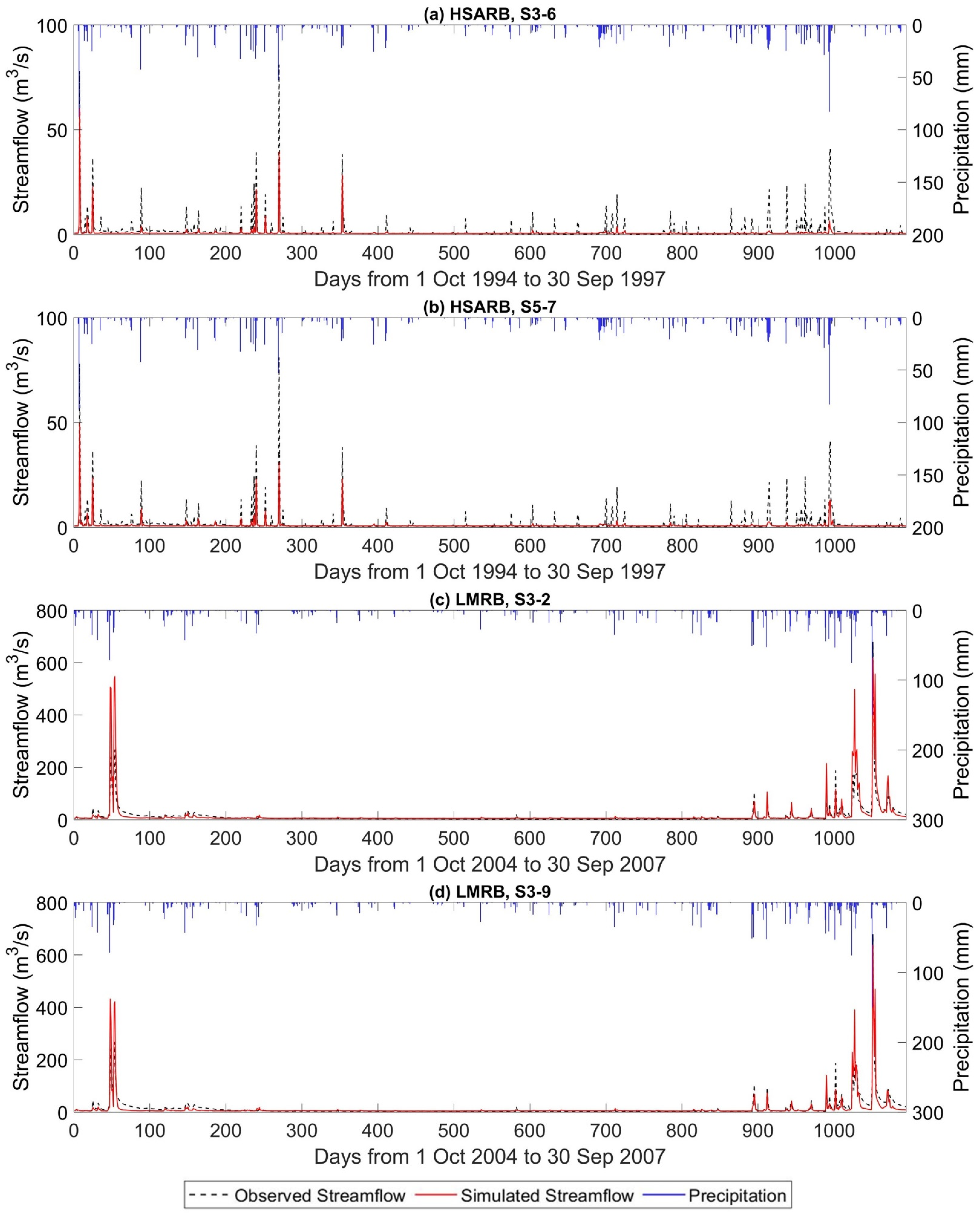
To better understand the difference between the models selected from different criteria and further assess their predictive performance, Figure 5 and Figure 6 present the testing phase streamflow time series and scatter plots for the best models selected by AIC, BIC, and BlockedCV. A closer inspection of the hydrographs (Figure 5) shows that the selected models can capture the timing of major peaks in both watersheds. However, the simulated and observed time series show apparent deviations in discharge magnitude for all models. For example, in the HSARB, both S3-6 and S5-7 underestimate the peak flows, whereas the fit of low flows is barely discernable due to the large vertical scales of the time series graphs. Conversely, both models S3-2 and S3-9 of the LMRB overestimated the peak flows. In the meantime, the time series graphs fail to provide valuable insights for the low flows as well.
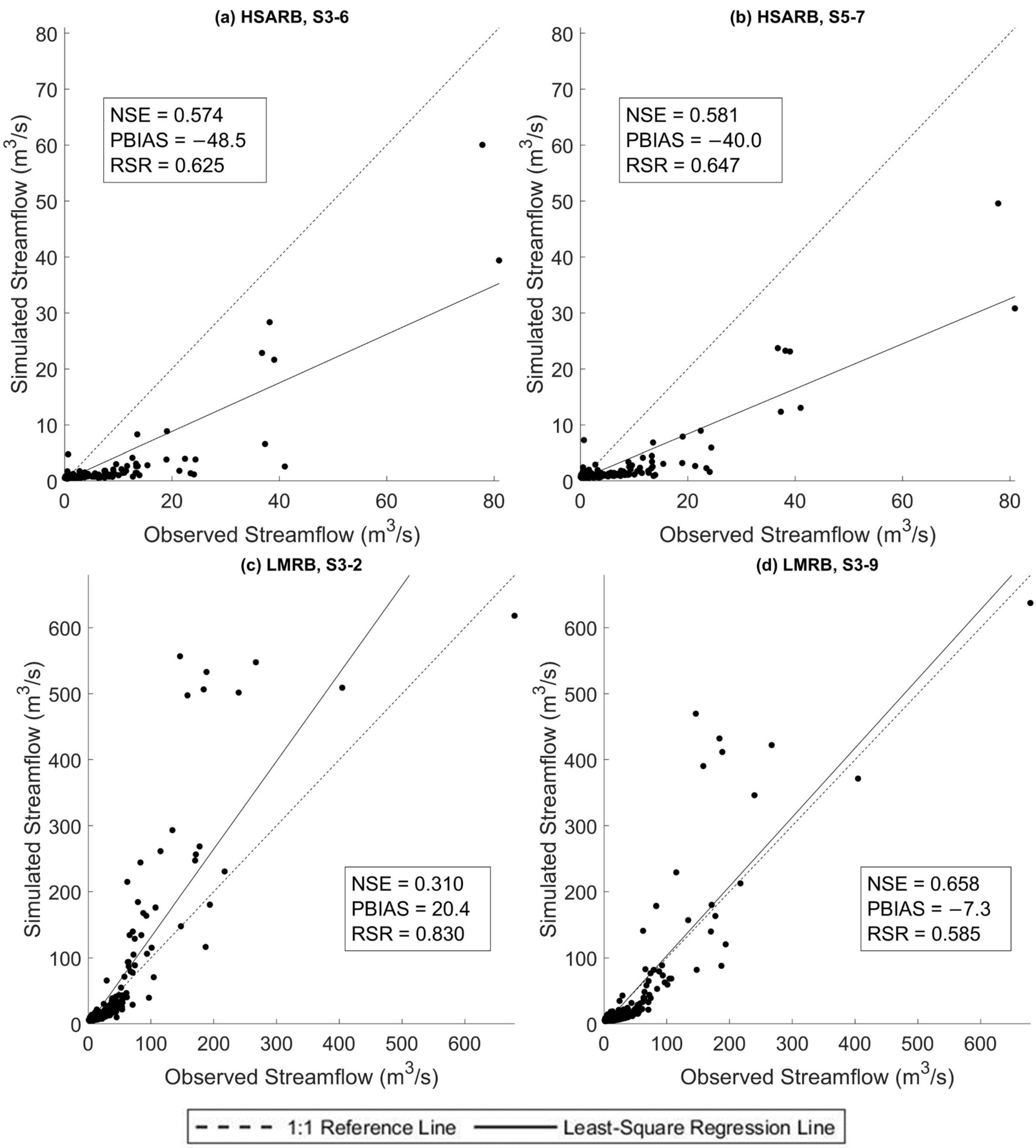
As noted by Moriasi et al. [51], although a time series plot is an effective graphical measure for evaluating event-specific prediction issues and allows the modeler to find possible temporal mismatches, it can become cluttered with too many data points. Hence, scatter plots should be applied for analyzing longer-duration datasets. Plots a,b of Figure 6 show the simulated against observed streamflow data of models S3-6 and S5-7 of the HSARB, and both plots suggest the models underestimate the observed streamflow with least-square regression lines that have slopes smaller than one. Meanwhile, the significant negative PBIAS values that were observed for both model S3-6 and S5-7 strengthen the graphic result that the ANN models in the HSARB underestimated streamflow. Plots c,d provide the scatter plots of models S3-2 and S3-9 of the LMRB. For model S3-2, the regression line has a slope greater than one and a positive PBIAS value, which indicates an apparent overestimation of streamflow. Much better performance is observed for model S3-9 of the LMRB, with a regression line that is the closest to the 1:1 reference line among the four models and a slight negative PBIAS value, which indicates the streamflow is slightly underestimated overall.
The testing phase performance results of the four selected models are displayed in Figure 6 as well. In the HSARB, the models selected from the two approaches have close performance results. More specifically, the BlockedCV selected model S5-7 obtained slightly better NSE and PBIAS and slightly worse RSR results than the AIC and BIC selected model S3-6. However, in the LMRB, all three performance measures indicate that the BlockedCV selected model, S3-9, has significantly better performance than the AIC and BIC selected model S3-2. In both study watersheds, the best models selected by the in-sample AIC and BIC criteria are simpler than the models selected by the out-of-sample BlockedCV approach. As mentioned in Section 3.2, the in-sample approach tends to select smaller hidden layer sizes than the out-of-sample approach. These results corroborate the ideas of Qi and Zhang [22], who suggested that the in-sample model selection criteria may over-penalize the model complexity and select models that underfit the data.
An interesting finding on the selected best models is that the model S3-9 of the LMRB has better performance in statistical and graphical measures than the model S5-7 of the HSARB. This result is contrary to the expectation that ANNs would have the better predictive ability in an urban watershed, where its dominant impervious surface causes more direct rainfall–runoff relation than in a nonurban watershed where the rainfall–runoff process is more complex. A possible explanation might be that the LMRB has a much higher average outflow volume than the HSARB (Figure 5 and Figure 6). Prior studies have noted that the ANN models produce better simulation results estimating high flows [5,7,53].
4. Summary and Conclusions
In this study, daily streamflow simulation models were developed for two small watersheds with distinctive land cover types in south-central Texas, using a three-layer feed-forward neural network. Five prediction scenarios using different combinations of meteorological and hydrological variables were considered, and for each prediction scenario a range of nodes in the hidden layer was evaluated. The results show that the best networks could produce “satisfactory” to “good” daily streamflow prediction performances for most of the considered input combinations. While plenty of studies have reported applying ANNs to H/WQ modeling, the model overfitting problem and model selection method for a hydrological time series simulation have not been adequately addressed.
This study empirically investigated two main approaches for selecting the best ANN rainfall–streamflow models: the in-sample approach using AIC and BIC as criteria and the out-of-sample approach using BlockedCV. The evidence from this study suggests that none of the proposed approaches consistently select the model that has the best testing dataset predictive ability based on the criteria of optimum hidden layer size. However, when considering selecting among predictive scenarios where model structure difference is more notable, it is found that BlockedCV is more capable of identifying the best predictive model. Furthermore, the AIC and BIC are also found to select a simpler model structure than BlockedCV. Overall, this study strengthens the idea that the in-sample model selection criteria may over-penalize model complexity and select models that underfit the data for modeling a streamflow time series. The final best models in both study watersheds selected through BlockedCV are found to have “good” performance on the testing data. However, a closer inspection of the scatter plots and corresponding PBIAS values indicates that the models can perform very differently on low and high flow data, especially in the LMRB. This finding is also supported by the counter-intuitive result that the largely rural LMRB has better model performance than the urban HSARB, which could be explained by the fact that the HSARB has a much smaller average outflow discharge than the LMRB. Further studies could assess the model selection criteria separately on different quantiles and magnitudes of the flow data while choosing watersheds with closer average flow volume for comparison.
Author Contributions
X.M. and P.K.S. contributed significantly to developing the methodology applied in this study. X.M. conducted the model simulations and wrote the original draft. X.M. and P.K.S. analyzed the results and revised the manuscript. All authors have read and agreed to the published version of the manuscript.
Funding
This research received no external funding.
Institutional Review Board Statement
Not applicable.
Informed Consent Statement
Not applicable.
Data Availability Statement
The data presented in this study are available on request from the corresponding author.
Acknowledgments
The first author was supported by the Texas A&M University Department of Water Management & Hydrological Science and the Department of Biological & Agricultural Engineering annual scholarship.
Conflicts of Interest
The authors declare no conflict of interest.
References
- Wurbs, R.A.; James, W.P. Water Resources Engineering; Prentice Hall: Upper Saddle River, NJ, USA, 2002. [Google Scholar]
- Fernandez, G.P.; Chescheir, G.M.; Skaggs, R.W.; Amatya, D.M. Development and testing of watershed-scale models for poorly drained soils. Trans. ASAE 2005, 48, 639–652. [Google Scholar] [CrossRef]
- Worland, S.C.; Steinschneider, S.; Asquith, W.; Knight, R.; Wieczorek, M. Prediction and Inference of Flow Duration Curves Using Multioutput Neural Networks. Water Resour. Res. 2019, 55, 6850–6868. [Google Scholar] [CrossRef] [Green Version]
- Maier, H.R.; Dandy, G.C. Neural networks for the prediction and forecasting of water resources variables: A review of modelling issues and applications. Environ. Model. Softw. 2000, 15, 101–124. [Google Scholar] [CrossRef]
- Humphrey, G.B.; Gibbs, M.S.; Dandy, G.C.; Maier, H.R. A hybrid approach to monthly streamflow forecasting: Integrating hydrological model outputs into a Bayesian artificial neural network. J. Hydrol. 2016, 540, 623–640. [Google Scholar] [CrossRef]
- Govindaraju, R.S.; Rao, A.R. Artificial Neural Networks in Hydrology; Springer Science & Business Media: Berlin/Heidelberg, Germany, 2013; Volume 36. [Google Scholar]
- Jimeno-Sáez, P.; Senent-Aparicio, J.; Pérez-Sánchez, J.; Pulido-Velazquez, D. A Comparison of SWAT and ANN models for daily runoff simulation in different climatic zones of peninsular Spain. Water 2018, 10, 192. [Google Scholar] [CrossRef] [Green Version]
- Minns, A.; Hall, M. Artificial neural networks as rainfall-runoff models. Hydrol. Sci. J. 1996, 41, 399–417. [Google Scholar] [CrossRef]
- Yaseen, Z.M.; El-Shafie, A.; Jaafar, O.; Afan, H.A.; Sayl, K.N. Artificial intelligence based models for stream-flow forecasting: 2000–2015. J. Hydrol. 2015, 530, 829–844. [Google Scholar] [CrossRef]
- ASCE. Artificial neural networks in hydrology. I: Preliminary concepts. J. Hydrol. Eng. 2000, 5, 115–123. [Google Scholar] [CrossRef]
- Ha, H.; Stenstrom, M.K. Identification of land use with water quality data in stormwater using a neural network. Water Res. 2003, 37, 4222–4230. [Google Scholar] [CrossRef]
- Jain, A.; Srinivasulu, S. Development of effective and efficient rainfall-runoff models using integration of deterministic, real-coded genetic algorithms and artificial neural network techniques. Water Resour. Res. 2004, 40. [Google Scholar] [CrossRef]
- Karunanithi, N.; Grenney, W.J.; Whitley, D.; Bovee, K. Neural networks for river flow prediction. J. Comput. Civ. Eng. 1994, 8, 201–220. [Google Scholar] [CrossRef]
- Ahmed, J.A.; Sarma, A.K. Artificial neural network model for synthetic streamflow generation. Water Resour. Manag. 2007, 21, 1015–1029. [Google Scholar] [CrossRef]
- Birikundavyi, S.; Labib, R.; Trung, H.; Rousselle, J. Performance of neural networks in daily streamflow forecasting. J. Hydrol. Eng. 2002, 7, 392–398. [Google Scholar] [CrossRef]
- Hu, T.; Lam, K.; Ng, S. River flow time series prediction with a range-dependent neural network. Hydrol. Sci. J. 2001, 46, 729–745. [Google Scholar] [CrossRef] [Green Version]
- Isik, S.; Kalin, L.; Schoonover, J.E.; Srivastava, P.; Lockaby, B.G. Modeling effects of changing land use/cover on daily streamflow: An artificial neural network and curve number based hybrid approach. J. Hydrol. 2013, 485, 103–112. [Google Scholar] [CrossRef]
- Kişi, Ö. Streamflow forecasting using different artificial neural network algorithms. J. Hydrol. Eng. 2007, 12, 532–539. [Google Scholar] [CrossRef]
- Rezaeianzadeh, M.; Stein, A.; Tabari, H.; Abghari, H.; Jalalkamali, N.; Hosseinipour, E.; Singh, V. Assessment of a conceptual hydrological model and artificial neural networks for daily outflows forecasting. Int. J. Environ. Sci. Technol. 2013, 10, 1181–1192. [Google Scholar] [CrossRef] [Green Version]
- Zhang, G.P.; Qi, M. Neural network forecasting for seasonal and trend time series. Eur. J. Oper. Res. 2005, 160, 501–514. [Google Scholar] [CrossRef]
- Donate, J.P.; Cortez, P.; SáNchez, G.G.; De Miguel, A.S. Time series forecasting using a weighted cross-validation evolutionary artificial neural network ensemble. Neurocomputing 2013, 109, 27–32. [Google Scholar] [CrossRef] [Green Version]
- Qi, M.; Zhang, G.P. An investigation of model selection criteria for neural network time series forecasting. Eur. J. Oper. Res. 2001, 132, 666–680. [Google Scholar] [CrossRef]
- Tashman, L.J. Out-of-sample tests of forecasting accuracy: An analysis and review. Int. J. Forecast. 2000, 16, 437–450. [Google Scholar] [CrossRef]
- Arlot, S.; Celisse, A. A survey of cross-validation procedures for model selection. Stat. Surv. 2010, 4, 40–79. [Google Scholar] [CrossRef]
- Shao, J. An asymptotic theory for linear model selection. Stat. Sin. 1997, 7, 221–242. [Google Scholar]
- Bergmeir, C.; Benítez, J.M. On the use of cross-validation for time series predictor evaluation. Inf. Sci. 2012, 191, 192–213. [Google Scholar] [CrossRef]
- Joseph, J.F.; Falcon, H.E.; Sharif, H.O. Hydrologic trends and correlations in south Texas River basins: 1950–2009. J. Hydrol. Eng. 2013, 18, 1653–1662. [Google Scholar] [CrossRef]
- Kreuter, U.P.; Harris, H.G.; Matlock, M.D.; Lacey, R.E. Change in ecosystem service values in the San Antonio area, Texas. Ecol. Econ. 2001, 39, 333–346. [Google Scholar] [CrossRef]
- Zhao, G.; Gao, H.; Cuo, L. Effects of urbanization and climate change on peak flows over the San Antonio River Basin, Texas. J. Hydrometeorol. 2016, 17, 2371–2389. [Google Scholar] [CrossRef]
- Yang, L.; Jin, S.; Danielson, P.; Homer, C.; Gass, L.; Bender, S.M.; Case, A.; Costello, C.; Dewitz, J.; Fry, J. A new generation of the United States National Land Cover Database: Requirements, research priorities, design, and implementation strategies. ISPRS J. Photogramm. Remote Sens. 2018, 146, 108–123. [Google Scholar] [CrossRef]
- Daly, C.; Halbleib, M.; Smith, J.I.; Gibson, W.P.; Doggett, M.K.; Taylor, G.H.; Curtis, J.; Pasteris, P.P. Physiographically sensitive mapping of climatological temperature and precipitation across the conterminous United States. Int. J. Climatol. 2008, 28, 2031–2064. [Google Scholar] [CrossRef]
- Gorelick, N.; Hancher, M.; Dixon, M.; Ilyushchenko, S.; Thau, D.; Moore, R. Google Earth Engine: Planetary-scale geospatial analysis for everyone. Remote Sens. Environ. 2017, 202, 18–27. [Google Scholar] [CrossRef]
- U.S. Geological Survey. National Water Information System Data Available on the World Wide Web (USGS Water Data for the Nation). Available online: https://waterdata.usgs.gov/nwis (accessed on 24 April 2020).
- Gupta, H.; Hsu, K.; Sorooshian, S. Effective and efficient modeling for streamflow forecasting. In Artificial Neural Networks in Hydrology; Springer: Berlin/Heidelberg, Germany, 2000; pp. 7–22. [Google Scholar]
- Zhang, B.; Govindaraju, R.S. Prediction of watershed runoff using Bayesian concepts and modular neural networks. Water Resour. Res. 2000, 36, 753–762. [Google Scholar] [CrossRef]
- Hastie, T.; Tibshirani, R.; Friedman, J. The Elements of Statistical Learning: Data Mining, Inference, and Prediction; Springer Science & Business Media: Berlin/Heidelberg, Germany, 2009. [Google Scholar]
- Srivastava, P.; McNair, J.N.; Johnson, T.E. Comparison of process-based and artificial neural network approaches for streamflow modeling in an agricultural watershed. J. Am. Water Resour. Assoc. 2006, 42, 545–563. [Google Scholar] [CrossRef]
- Amiri, B.; Sudheer, K.; Fohrer, N. Linkage between in-stream total phosphorus and land cover in Chugoku district, Japan: An ANN approach. J. Hydrol. Hydromech. 2012, 60, 33–44. [Google Scholar] [CrossRef] [Green Version]
- Gazzaz, N.M.; Yusoff, M.K.; Aris, A.Z.; Juahir, H.; Ramli, M.F. Artificial neural network modeling of the water quality index for Kinta River (Malaysia) using water quality variables as predictors. Mar. Pollut. Bull. 2012, 64, 2409–2420. [Google Scholar] [CrossRef] [PubMed]
- Kim, M.; Baek, S.; Ligaray, M.; Pyo, J.; Park, M.; Cho, K. Comparative studies of different imputation methods for recovering streamflow observation. Water 2015, 7, 6847–6860. [Google Scholar] [CrossRef] [Green Version]
- Maier, H.R.; Dandy, G.C. The use of artificial neural networks for the prediction of water quality parameters. Water Resour. Res. 1996, 32, 1013–1022. [Google Scholar] [CrossRef]
- James, G.; Witten, D.; Hastie, T.; Tibshirani, R. An introduction to Statistical Learning; Springer: Berlin/Heidelberg, Germany, 2013; Volume 112. [Google Scholar]
- Sheather, S. A Modern Approach to Regression with R; Springer Science & Business Media: Berlin/Heidelberg, Germany, 2009. [Google Scholar]
- Akaike, H. A new look at the statistical model identification. In Selected Papers of Hirotugu Akaike; Springer: Berlin/Heidelberg, Germany, 1974; pp. 215–222. [Google Scholar]
- Nash, J.E.; Sutcliffe, J.V. River flow forecasting through conceptual models part I—A discussion of principles. J. Hydrol. 1970, 10, 282–290. [Google Scholar] [CrossRef]
- Zhang, X.; Srinivasan, R.; Zhao, K.; Liew, M.V. Evaluation of global optimization algorithms for parameter calibration of a computationally intensive hydrologic model. Hydrol. Process. 2009, 23, 430–441. [Google Scholar] [CrossRef]
- Zhang, X.; Srinivasan, R.; Liew, M.V. On the use of multi-algorithm, genetically adaptive multi-objective method for multi-site calibration of the SWAT model. Hydrol. Process. 2010, 24, 955–969. [Google Scholar] [CrossRef]
- Moriasi, D.N.; Arnold, J.G.; Van Liew, M.W.; Bingner, R.L.; Harmel, R.D.; Veith, T.L. Model evaluation guidelines for systematic quantification of accuracy in watershed simulations. Trans. ASABE 2007, 50, 885–900. [Google Scholar] [CrossRef]
- Kalin, L.; Isik, S.; Schoonover, J.E.; Lockaby, B.G. Predicting water quality in unmonitored watersheds using artificial neural networks. J. Environ. Qual. 2010, 39, 1429–1440. [Google Scholar] [CrossRef] [PubMed]
- ASABE. Guidelines for Calibrating, Validating, and Evaluating Hydrologic and Water Quality (H/WQ) Models; ASABE: St. Joseph, MI, USA, 2017. [Google Scholar]
- Moriasi, D.N.; Gitau, M.W.; Pai, N.; Daggupati, P. Hydrologic and water quality models: Performance measures and evaluation criteria. Trans. ASABE 2015, 58, 1763–1785. [Google Scholar]
- Noori, N.; Kalin, L. Coupling SWAT and ANN models for enhanced daily streamflow prediction. J. Hydrol. 2016, 533, 141–151. [Google Scholar] [CrossRef]
- Demirel, M.C.; Venancio, A.; Kahya, E. Flow forecast by SWAT model and ANN in Pracana basin, Portugal. Adv. Eng. Softw. 2009, 40, 467–473. [Google Scholar] [CrossRef]
- Dorofki, M.; Elshafie, A.H.; Jaafar, O.; Karim, O.A.; Mastura, S. Comparison of artificial neural network transfer functions abilities to simulate extreme runoff data. Int. Proc. Chem. Biol. Environ. Eng. 2012, 33, 39–44. [Google Scholar]
- Maraun, D.; Wetterhall, F.; Ireson, A.; Chandler, R.; Kendon, E.; Widmann, M.; Brienen, S.; Rust, H.; Sauter, T.; Themeßl, M. Precipitation downscaling under climate change: Recent developments to bridge the gap between dynamical models and the end user. Rev. Geophys. 2010, 48. [Google Scholar] [CrossRef]
- Cox, D.R.; Stuart, A. Some quick sign tests for trend in location and dispersion. Biometrika 1955, 42, 80–95. [Google Scholar] [CrossRef] [Green Version]
- Sahoo, G.; Ray, C. Flow forecasting for a Hawaii stream using rating curves and neural networks. J. Hydrol. 2006, 317, 63–80. [Google Scholar] [CrossRef]
- Starrett, S.K.; Starrett, S.K.; Heier, T.; Su, Y.; Tuan, D.; Bandurraga, M.J.A.J.o.E.; Sciences, A. Filling in missing peak flow data using artificial neural networks. ARPN J. Eng. Appl. Sci. 2010, 5, 49–55. [Google Scholar]
- R Core Team. R: A Language and Environment for Statistical Computing; R Foundation for Statistical Computing: Vienna, Austria, 2019. [Google Scholar]
Figure 1.
Study Area, the headwaters San Antonio River Basin (HSARB), and the Lower Medina River Basin (LMRB) with NLCD LULC classification and USGS Stream Gages displayed.
Figure 1.
Study Area, the headwaters San Antonio River Basin (HSARB), and the Lower Medina River Basin (LMRB) with NLCD LULC classification and USGS Stream Gages displayed.

Figure 2.
Schematic diagram of the blocked cross-validation.

Figure 3.
Model statistical performance of prediction scenarios 1 through 5 for the HSARB watershed (a−e). The best performance measures of each scenario (i.e., the smallest AIC and BIC, the largest NSE) are highlighted in red.
Figure 3.
Model statistical performance of prediction scenarios 1 through 5 for the HSARB watershed (a−e). The best performance measures of each scenario (i.e., the smallest AIC and BIC, the largest NSE) are highlighted in red.

Figure 4.
Model statistical performance of prediction scenarios 1 through 5 for the LMRB watershed (a−e). The best performance measures of each scenario (i.e., the smallest AIC and BIC, the largest NSE) are highlighted in red.
Figure 4.
Model statistical performance of prediction scenarios 1 through 5 for the LMRB watershed (a−e). The best performance measures of each scenario (i.e., the smallest AIC and BIC, the largest NSE) are highlighted in red.

Figure 5.
Daily precipitation, observed, and simulated streamflow of testing phase for (a) HSARB, S3-6; (b) HSARB, S5-7; (c) LMRB S3-2; (d) LMRB S3-9.
Figure 5.
Daily precipitation, observed, and simulated streamflow of testing phase for (a) HSARB, S3-6; (b) HSARB, S5-7; (c) LMRB S3-2; (d) LMRB S3-9.

Figure 6.
Scatter plots of testing phase daily streamflow of (a) HSARB, S3-6; (b) HSARB, S5-7; (c) LMRB S3-2; (d) LMRB S3-9.
Figure 6.
Scatter plots of testing phase daily streamflow of (a) HSARB, S3-6; (b) HSARB, S5-7; (c) LMRB S3-2; (d) LMRB S3-9.


Table 1.
Model performance evaluation criteria.
| Performance Rating | NSE | PBIAS (%) | RSR |
|---|---|---|---|
| Very good | |||
| Good | |||
| Satisfactory | |||
| Unsatisfactory |
Table 2.
ANN model input combinations.
| Prediction Scenario | Input Combination | Output |
|---|---|---|
| 1 | Pt, Pt−1, Pt−2, Pt−3, Pt−4, Qu | Q |
| 2 | Pt, Pt−1, Pt−2, Pt−3, Pt−4, Tt | Q |
| 3 | Pt, Pt−1, Pt−2, Pt−3, Pt−4, Tt, Qu | Q |
| 4 | Pt, Pt−1, Pt−2, Pt−3, Pt−4, Pn | Q |
| 5 | Pt, Pt−1, Pt−2, Pt−3, Pt−4, Pn, Qu | Q |
Table 3.
AIC selected models with the optimum number of hidden nodes, HSARB.
| Scenario | Hidden Nodes | Training | Testing | ||||||
|---|---|---|---|---|---|---|---|---|---|
| AIC | BIC | NSE | PBIAS | RSR | NSE | PBIAS | RSR | ||
| 1 | 5 | 10.299 | 10.397 | 0.841 | 10.8 | 0.399 | 0.558 | −47.8 | 0.664 |
| 2 | 3 | 11.393 | 11.453 | 0.519 | 9.9 | 0.694 | 0.474 | −36.7 | 0.725 |
| 3 | 6 | 10.258 | 10.389 | 0.849 | 8.6 | 0.388 | 0.574 | −48.5 | 0.652 |
| 4 | 5 | 11.406 | 11.504 | 0.519 | 11.1 | 0.694 | 0.512 | −31.8 | 0.698 |
| 5 | 4 | 10.337 | 10.425 | 0.834 | 9.4 | 0.407 | 0.577 | −45.7 | 0.650 |
Table 4.
BlockedCV selected models with the optimum number of hidden nodes, HSARB.
| Scenario | Hidden Nodes | Training | Validation | Testing | ||||||
|---|---|---|---|---|---|---|---|---|---|---|
| NSE | PBIAS | RSR | NSE | PBIAS | RSR | NSE | PBIAS | RSR | ||
| 1 | 4 | 0.774 | 11.3 | 0.474 | 0.707 | 29.6 | 0.538 | 0.566 | −48.8 | 0.659 |
| 2 | 10 | 0.537 | 8.8 | 0.680 | −0.229 | 65.7 | 1.105 | 0.465 | −36.8 | 0.731 |
| 3 | 7 | 0.764 | 11.5 | 0.486 | 0.690 | 33.7 | 0.555 | 0.567 | −47.6 | 0.658 |
| 4 | 10 | 0.525 | 10.6 | 0.689 | −0.106 | 62.3 | 1.049 | 0.478 | −30.5 | 0.723 |
| 5 | 7 | 0.790 | 11.4 | 0.457 | 0.717 | 31.3 | 0.529 | 0.581 | −40.0 | 0.647 |
Table 5.
AIC selected models with the optimum number of hidden nodes, LMRB.
| Scenario | Hidden Nodes | Training | Testing | ||||||
|---|---|---|---|---|---|---|---|---|---|
| AIC | BIC | NSE | PBIAS | RSR | NSE | PBIAS | RSR | ||
| 1 | 2 | 12.707 | 12.746 | 0.920 | 16.2 | 0.282 | 0.269 | 18.8 | 0.854 |
| 2 | 4 | 13.559 | 13.634 | 0.816 | −10.8 | 0.429 | 0.451 | −58.6 | 0.741 |
| 3 | 2 | 12.666 | 12.710 | 0.924 | 15.2 | 0.276 | 0.310 | 20.4 | 0.830 |
| 4 | 7 | 13.488 | 13.618 | 0.831 | −15.2 | 0.411 | 0.603 | −47.9 | 0.630 |
| 5 | 5 | 12.779 | 12.884 | 0.916 | 10.4 | 0.289 | 0.400 | 4.6 | 0.775 |
Table 6.
BlockedCV selected models with the optimum number of hidden nodes, LMRB.
| Scenario | Hidden Nodes | Training | Validation | Testing | ||||||
|---|---|---|---|---|---|---|---|---|---|---|
| NSE | PBIAS | RSR | NSE | PBIAS | RSR | NSE | PBIAS | RSR | ||
| 1 | 8 | 0.920 | 14.0 | 0.283 | 0.282 | −35.0 | 0.845 | 0.574 | 3.5 | 0.653 |
| 2 | 8 | 0.817 | −11.9 | 0.427 | 0.115 | −53.0 | 0.939 | 0.444 | −61.5 | 0.745 |
| 3 | 9 | 0.916 | 16.6 | 0.290 | 0.290 | −32.8 | 0.841 | 0.658 | −7.3 | 0.585 |
| 4 | 9 | 0.817 | −11.7 | 0.427 | 0.066 | −54.6 | 0.964 | 0.582 | −48.7 | 0.647 |
| 5 | 10 | 0.916 | 13.8 | 0.289 | 0.283 | −35.2 | 0.845 | 0.320 | 11.6 | 0.824 |
Table 7.
Selected best model structure with different criteria.
| Study Watershed | Selection Criteria | Best Model | Study Watershed | Selection Criteria | Best Model |
|---|---|---|---|---|---|
| HSARB | AIC | S3-6 | LMRB | AIC | S3-2 |
| BIC | S3-6 | BIC | S3-2 | ||
| BlockedCV | S5-7 | BlockedCV | S3-9 | ||
| Predictive Performance | S5-5 | Predictive Performance | S3-9 |
Publisher’s Note: MDPI stays neutral with regard to jurisdictional claims in published maps and institutional affiliations. |
© 2021 by the authors. Licensee MDPI, Basel, Switzerland. This article is an open access article distributed under the terms and conditions of the Creative Commons Attribution (CC BY) license (https://creativecommons.org/licenses/by/4.0/).
Share and Cite
MDPI and ACS Style
Mei, X.; Smith, P.K. A Comparison of In-Sample and Out-of-Sample Model Selection Approaches for Artificial Neural Network (ANN) Daily Streamflow Simulation. Water 2021, 13, 2525. https://doi.org/10.3390/w13182525
AMA Style
Mei X, Smith PK. A Comparison of In-Sample and Out-of-Sample Model Selection Approaches for Artificial Neural Network (ANN) Daily Streamflow Simulation. Water. 2021; 13(18):2525. https://doi.org/10.3390/w13182525
Chicago/Turabian StyleMei, Xiaohan, and Patricia K. Smith. 2021. "A Comparison of In-Sample and Out-of-Sample Model Selection Approaches for Artificial Neural Network (ANN) Daily Streamflow Simulation" Water 13, no. 18: 2525. https://doi.org/10.3390/w13182525
Note that from the first issue of 2016, this journal uses article numbers instead of page numbers. See further details here.