
Characterization of Bias during Meteorological Drought Calculation in Time Series Out-of-Sample Validation


Department of Environment, University of the Aegean, 81100 Mytilene, Greece
*
Author to whom correspondence should be addressed.
Water 2021, 13(18), 2531; https://doi.org/10.3390/w13182531
Submission received: 3 August 2021
/
Revised: 9 September 2021
/
Accepted: 10 September 2021
/
Published: 15 September 2021
(This article belongs to the Special Issue Assessing Hydrological Drought in a Climate Change: Methods and Measures)
Abstract
:The standardized precipitation index (SPI) is used for characterizing and predicting meteorological droughts on a range of time scales. However, in forecasting applications, when SPI is computed on the entire available dataset, prior to model-validation, significant biases are introduced, especially under changing climatic conditions. In this paper, we investigate the theoretical and numerical implications that arise when SPI is computed under stationary and non-stationary probability distributions. We demonstrate that both the stationary SPI and non-stationary SPI (NSPI) lead to increased information leakage to the training set with increased scales, which significantly affects the characterization of drought severity. The analysis is performed across about 36,500 basins in Sweden, and indicates that the stationary SPI is unable to capture the increased rainfall trend during the last decades and leads to systematic underestimation of wet events in the training set, affecting up to 22% of the drought events. NSPI captures the non-stationary characteristics of accumulated rainfall; however, it introduces biases to the training data affecting 19% of the drought events. The variability of NSPI bias has also been observed along the country’s climatic gradient with regions in snow climates strongly being affected. The findings propose that drought assessments under changing climatic conditions can be significantly influenced by the potential misuse of both SPI and NSPI, inducing bias in the characterization of drought events in the training data.
1. Introduction
Droughts have significant environmental and socio-economic impacts comparable to other hazards, including floods, landslides, and earthquakes. In particular, the total economic damage of natural disasters during the 2003–2013 decade was estimated at USD 1.53 trillion [1], whilst the economic losses from droughts in Europe and the United Kingdom are expected to increase due to global warming between EUR 9.7 billion (under a +1.5 C warming) and EUR 17.3 billion per year (under a +3 C warming) [2]. Consequently, a variety of drought risk mitigation measures have been employed during the last decades in drought-sensitive sectors, including, for example, drought-resistant crops for agriculture, improved cooling techniques for health and early warning alerting systems for emergency management [2]. In addition, the Copernicus Emergency Management Service launched the European and Global Drought Observatories to improve preparedness by monitoring the occurrence and severity of droughts and forecasting the meteorological drought with a 3-month lead time [3].
The standardized precipitation index (SPI; [4]) has been widely used in early warning and climate services for the estimation of the onset, duration, and intensity of meteorological drought [5,6]. SPI expresses the accumulated precipitation over a specific period as a departure from the precipitation probability distribution and is very popular due to its simplicity; with only precipitation being required as input. It can be computed in different time scales (usually 3 to 24 months, indicated as SPI(3) to SPI(24), respectively) and can capture different aspects of the meteorological drought ranging from short- to long-term scales [7,8,9,10]. SPI(1) to SPI(3) address short accumulated periods and indicate relatively immediate precipitation responses such as reduction in soil moisture and snowpack. SPI(3) to SPI(12) address medium accumulation periods and indicate changes in seasonality of streamflow and reservoir storage [11]. For long accumulation periods, SPI(12) to SPI(48) are used to assess changes in slow responding fluxes, such as groundwater recharge.
SPI requires fitting a probability density function to the accumulated precipitation series (see Section in the Appendix A), with the Gamma distribution being the most popular as it is simple and can very well describe the accumulated precipitation at various scales [12,13]. However, the selection of a distribution may introduce bias to the index values by introducing over-/under-estimated drought events [14]. Alternatively, the Log-Normal, Normal [15], exponatiated Weibull [16], and the generalized extreme values (GEV) [17] distributions have been considered in many cases. In a changing climate where precipitation exhibits non-stationarity, traditional SPI calculation involves fitting the accumulated precipitation to a time-invariant probability density function, resulting to a trending SPI series that reflects the trend of accumulated precipitation [18]. To avoid this limitation, different versions of a non-stationary standardized precipitation index (NSPI) have been proposed using a time-varying probability density function that models precipitation under climate change. Russo et al. [19] modeled precipitation data with a linear trend in the scale parameter of the Gamma distribution, using generalized linear models on climate projections of global climate models. Wang et al. [20] developed a time-dependent SPI by fitting generalized additive models in location, scale, and shape (GAMLSS) to monitor regional droughts during the summer period in the Luanhe River basin in China. Results suggested that under non-stationarity in precipitation, the use of the traditional SPI does not lead to accurate drought classification.
Nevertheless, there are many studies where the stationary SPI has been used thoroughly to forecast meteorological drought at different time scales. Stochastic linear models, such as the autoregressive integrated moving average (ARIMA) and the seasonal autoregressive moving average (SARIMA) [21], have been used for SPI forecasting in different climatic domains [22,23,24,25]. Although these models address the non-stationary characteristics of drought, their ability to forecast non-linear components of the time series is limited. Methods such as the support vector regression (SVR) [26] and the artificial neural network (ANN) [27] have shown potential in drought forecasting applications due to their ability to capture non-linearities in the time series. The performance of these models is generally comparable, and hence both SVR and ANN have been recommended for forecasting applications [28,29].
Despite SPI’s popularity in drought forecasting applications, the effect of the estimation of the index during model-validation has not been addressed until now. SPI is very sensitive to the temporal characteristics of precipitation and hence when computed on precipitation records at different accumulation periods, SPI leads to values with numerical differences. This is mainly due to the difference of the underlying probability distribution of precipitation from one period to another which increases in the long-term scales of the index [30]. In most studies that focus on drought forecasting applications, SPI has been computed on the entire dataset, omitting any model-validation for time-series, and further use of the validation and test datasets to estimate the respective distribution parameters [29,31,32,33]. In this case, the observations of SPI in the training dataset share the same parameter estimates with the validation and test datasets. This approach violates the fundamental principles of model-validation as accessing future information leads to different characterization of drought events in the training set, potentially enabling fitted models to access future information while it is not present.
Here, we investigate and quantify the complications related to incorrect computation of SPI, particularly with respect to climate change and the corresponding rainfall variability. Imprecise estimation of SPI, results to systematic biases leading to changes in the classification of drought events.The biases should not be ignored as they are propagated in the building process of any forecasting model. Most studies treat SPI as a traditional univariate sequence of observations, omitting the temporal dependence of the index on historical and future records [34,35]. Therefore, we note that drought forecasting is not the goal of this study, and instead, we address the violated fundamental principles of model-validation and pose the following scientific questions: (1) Are there any differences between the densities of accumulated precipitation when SPI is calculated using the entire data, prior to model-validation? (2) Are there deviations in drought events when stationary or non-stationary drought indices are computed? (3) Is the bias sensitive to the SPI scale? and (4) How does the bias vary in space depending on the underlying climate? To address these questions, we: (a) investigate the incorrect computation of SPI, (b) quantify the bias introduced to the index data when the SPI is computed prior to model-validation, and (c) assess the bias along a climatic gradient.
The paper is organized as follows. Section 2 presents a theoretical overview of model-validation for drought forecasting applications. Section 3 presents the proposed methodology. Section 4 presents the results, followed by a discussion in Section 5. Finally, in Section 6 we present the conclusions. The methodologies provided to calculate SPI and NSPI are provided in the Appendix A.
2. Theoretical Overview
2.1. Data Separation in Model-Validation for Time Series Forecasting
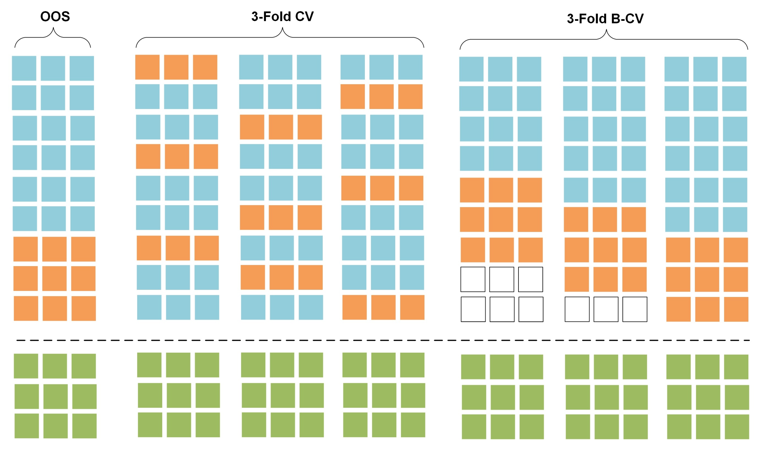
Two well-known model validation techniques are presented here; the out-of-sample (OOS) model-validation and the cross-validation (CV). OOS model-validation is the most common technique of data partitioning in traditional time series forecasting applications. The data are split into two different sets; the training set, which is used to train a model using a set of hyper-parameters and features, and the validation set, which is used to validate the model and it usually constitutes the last block of the series [36]. This approach preserves the temporal order of the series and copes with the dependency among observations (see Figure 1, OOS: train (blue), validation (orange)). Various extensions of the standard OOS validation approach have been introduced during the last years [37]; the fixed origin evaluation, within rolling-origin-recalibration evaluation, rolling-origin-update evaluation and rolling-window evaluation are some of the most important validation methods applied on individual series. However, using the last block of the series for model-validation does not always lead to a diverse validation error as the error reflects the characteristics of the series in the validation set, not present in the historical and future data [37].
CV is a statistical method that is used to evaluate the skill of regression and classification algorithms by measuring their performance on “unseen” datasets. It differs to the OOS validation method as the training and validation sets must cross-over in successive rounds, such that each data point has a chance of being validated. The k-fold cross validation is one of the most widely used approaches to assess the predictive performance of a model [38]. Here, the data are split into K roughly equal sized parts, while a model is fitted on the parts of the data, and the prediction error is evaluated on the Kth part. The prediction error is a combination of K individual predictive errors and is used to select the best model across a series of models trained using different hyper-parameters and features (see Figure 1, CV: train (blue), validation (orange)). In traditional time series forecasting, k-fold CV receives little attention due to the theoretical and practical implications that violate the temporal dependency of the series [37]. To avoid violations on the temporal dependence, the validation set needs to be chronologically placed after the training set [36]. Blocked-CV (B-CV) is a variation of the standard k-fold CV, where the data are not partitioned randomly but sequentially into K sets, preserving the temporal order of the series [37] (see Figure 1, train (blue), validation (orange)).
In both OOS and CV techniques, the test set should be kept in a vault (see Figure 1, test set is presented in yellow) and should be brought out at the end of the data analysis to perform model evaluation on unseen data (test error) as expected in real world applications [38].
In this study, we focus on the OOS model-validation method, since it is the key model-validation approach in drought forecasting applications [28], both for individual series analysis, regression and classification models. We denote the OOS model-validation function, , for time series forecasting tasks as follows:
Let be a vector of time series records with temporal dependence and length equal to M. Let also k: be an indexing function that indicates the training set and l: an indexing function that indicates the validation set such that . Denote the fitted function with the kth part of the data removed, and the function evaluated on the ith observation of the kth part of the data. Then the OOS model-validation estimate of the test error is defined as:
Given a set of models tuned by a parameter , denote the th model evaluated with the kth part of the data. Then, for this set of models we define:
The function provides an estimate of the test error and our goal is to find the tuning parameter that minimizes it. Let m: be an index that indicates the observations of the test set. The actual test error of the th model is given by:
2.2. Addressing the Effect of Bias during Model-Validation in Drought Forecasting Applications
Even though OOS model-validation and k-fold B-CV deal with the temporal characteristics of the time series, there are additional sources of bias that violate the model validation process when predicting SPI. As presented in several studies (among others, [32,39]), SPI is computed using the entire available dataset; this means that the associated probability distribution parameters are estimated using information from historical and future records. The SPI series is often non-stationary and the probability distribution of monthly precipitation changes over time. When the SPI records of the training set are influenced by the properties of the precipitation distribution in the validation and test sets then the model-validation estimate of the test error is biased as it accesses future information while it should not. In this paper, we address the source and the magnitude of bias introduced during model-validation by demonstrating three different versions of the index calculated on different subsets of the data. To do so, we formulate the model-validation function for each one of these cases.
Let be a time series of monthly precipitation records with length equal to M. Let also k: be an indexing function that indicates the training set, l: indicates the validation set and m: indicates the test set, respectively, such that . We denote by the SPI at scale s that is computed for three different subsets of the data:
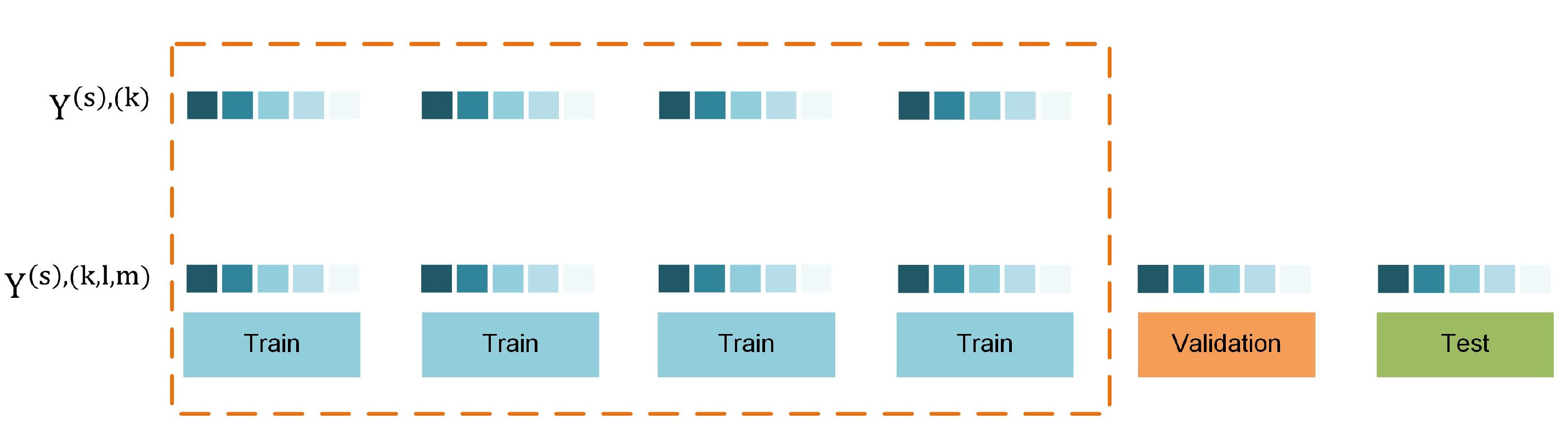
where being the different versions of SPI computed using the train , train and validation and train, validation and test sets, respectively (Figure 2). Consequently each version of the index is computed on data of different length. For each subset, a probability distribution function (e.g., Gamma, non-stationary Gamma) is fitted and its parameters are estimated to compute the SPI. Different lengths of data lead to different probability distribution functions [36] and subsequently to different SPI raw data, such that .
The model-validation function for each version of the SPI index is defined as follows:
where is the function evaluated on the validation set with index k and is the ith observation of the SPI index computed on the training set only (Equation (4)). The model-validation function of the SPI computed using the training and validation sets is given by:
where is the ith observation of the SPI. Equivalently, the model-validation function of the index computed on the training, validation, and test sets is as follows:
where is the ith observation of the index.
It is clear from the above definitions that different versions of SPI, with respect to data subsets, lead to different versions of the expected test error. The amount of bias introduced to the model-validation functions of Equations (8) and (9) is due to SPI’s dependency on the parameter estimates of future and historical precipitation records. This leads to information leakage through and . We call this information leakage of SPI introduced to the model-validation process in drought forecasting applications.
2.3. Estimating Bias during Model-Validation
The bias in SPI introduced from the data in the training set during model-validation is estimated by measuring the deviation between our baseline, (Equation (4)) and the SPI computed on the entire dataset, (Equation (6)). We employee different approaches that cover different aspects of the bias introduced to the distribution parameters in the training set: (1) the comparison between the distributions of accumulated precipitation that influence the estimation of drought in the training set, (2) the drought class transition approach that reflects potential changes in the characteristics of drought events, and (3) a set of statistical measures to quantify the deviation between the two versions of the index and generate insights when different scales are employed.
2.3.1. Comparison between the Distributions of Accumulated Precipitation
One of the main calculation steps of SPI, requires fitting a probability distribution function (e.g., Gamma, non-stationary Gamma) on the accumulated precipitation records for a given time scale. The parameters of the distribution are estimated using maximum likelihood and then the cumulative distribution is converted into a standard z-score (see Section in the Appendix A). When SPI is computed using the training, validation, and test data, then the probability distribution function is fitted on the entire data and this violates the fundamental principles of model-validation, described in Section 2.2. We compare the distribution parameter estimates between the two computational approaches of SPI, and , to conclude whether potential change in the accumulated precipitation introduces bias in the training data. We perform further analysis by comparing the densities of accumulated precipitation for individual months and stations and demonstrate our findings in Section 4.
2.3.2. Drought Class Transition
A drought class transition is defined as the change in the characterization of a drought event when SPI is computed using the entire available dataset , instead of the training set . By measuring drought class transitions , we aim at quantifying the magnitude of change in SPI classification with respect to the subsets used during model-validation (Figure 3). A transition from Moderately Wet when the is computed to Moderately Dry when the is instead computed suggests that the version of the SPI computed on the entire dataset incorporates bias to the training data by underestimating a wet event and classifying it as dry event.
2.3.3. Comparison between the Raw SPI Data
The mean absolute deviation (MAD) was used to quantify the amount of error introduced to the training data. MAD is a linear score that measures the average magnitude of the deviations from the mean:
where K is the total number of records in the training set, s is the scale of the SPI and are the index vectors for the training, validation and test sets, respectively.
3. Methodology
3.1. Data and Region of Interest
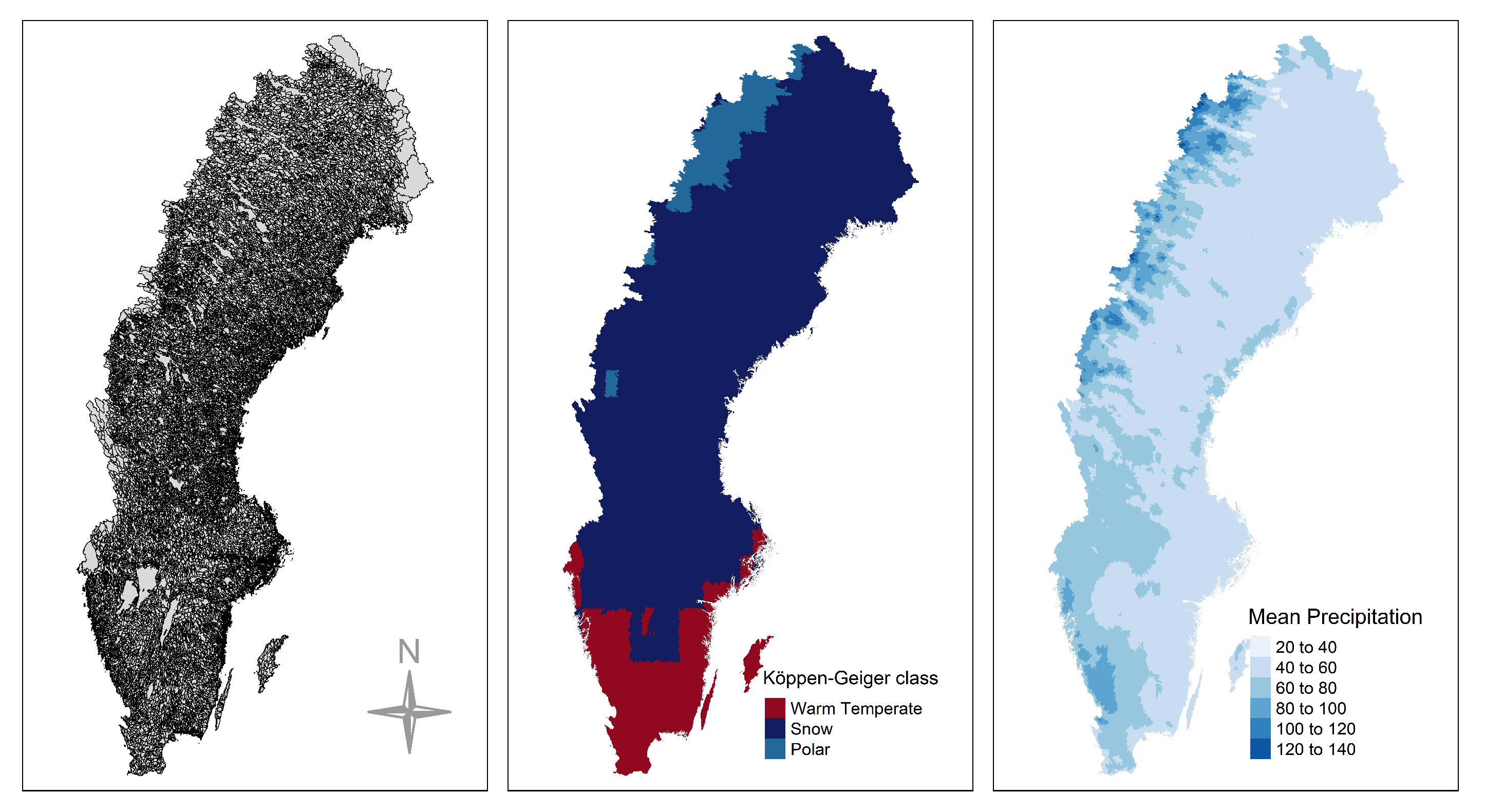
Sweden has a surface area of about 450,000 , with its climate being characterized by a strong spatial gradient and a seasonal pattern. Precipitation is high in the west (mountainous areas) and is gradually reduced eastwards. The climatic patterns over the country can be clustered into three regions according to the Köppen-Geiger climate classification system [40]; snow, polar, and warm temperate (Figure 4). Sweden receives precipitation between 500 and 800 mm/year; however in the southwestern part of the country precipitation ranges between 1000 and 1200 mm, whilst in mountainous areas in the north precipitation can reach up to 2000 mm. An extensive 58-years record of observed daily precipitation (1 January 1961 till 30 September 2018) over Sweden at 36,662 basins has been provided by the Swedish Meteorological and Hydrological Institute (SMHI) (see Figure 4). The precipitation is spatially interpolated from SMHI’s station network and elevation corrected to capture precipitation for hydrological applications at the basin scale [41]. This meteorological dataset is considered as state-of-the-art observation product in Sweden and has been used in various investigations, including seasonal forecasting and climate projections. These daily precipitation records were aggregated into monthly values, which were further used here.
3.2. Experimental Setup
A set of experiments were performed on the 36,662 basins using the available data to quantify the bias introduced to the training set. The analysis period is from January 1961 to September 2018 and each station consists of 693 monthly precipitation observations. At each location, the data were split into training (60%), validation (20%), and test (20%) sets using the OOS model-validation methodology described in Section 2.1. This ensures that the training set consists of at least 30 years of precipitation records to compute each version of SPI [4,42]. Two probability distribution functions were used: (1) the stationary Gamma, using maximum likelihood estimation, that leads to the computation of the traditional SPI (see Appendix A, Equations (A1)–(A7)), and (2) the non-stationary NS-Gamma (with time-varying location and scale parameters) that leads to the non-stationary SPI (NSPI) and is able to capture the increased precipitation trend during the last decades (see Appendix B). Additionally, different SPI scales were calculated (SPI(3), SPI(6), SPI(9), SPI(12), SPI(24)) to exploit potential relationships between the scale of the index and the level of bias introduced to the training set during model-validation. The two computational approaches of the SPI are employed; first, SPI is computed using only the training data, , and second, SPI is computed using the entire dataset (training, validation, and test), (see Figure 3). In our experiments, we treat as the baseline since it does not violate the fundamental assumptions of the OOS model-validation process eliminating information leakage. The analyses are performed in the training set to:
- Compare the densities of accumulated rainfall (see Section 2.3.1);
- Count the number of drought class transitions (see Section 2.3.2);
- Analyze the magnitude of the bias introduced at different SPI scales (see Section 2.3.3);
- Assess the variation of bias along Sweden’s climatic gradient. The error introduced to the model-validation is quantified based on one statistical metric; the mean absolute deviation (see Section 2.3.3).
Moreover, we showcase a set of experiments using data from a meteorological station the characteristics of which are presented in Table 1. It is clear that there is a change in the mean monthly precipitation between the two subsets.
4. Results
4.1. Comparison between the Distributions of Accumulated Precipitation
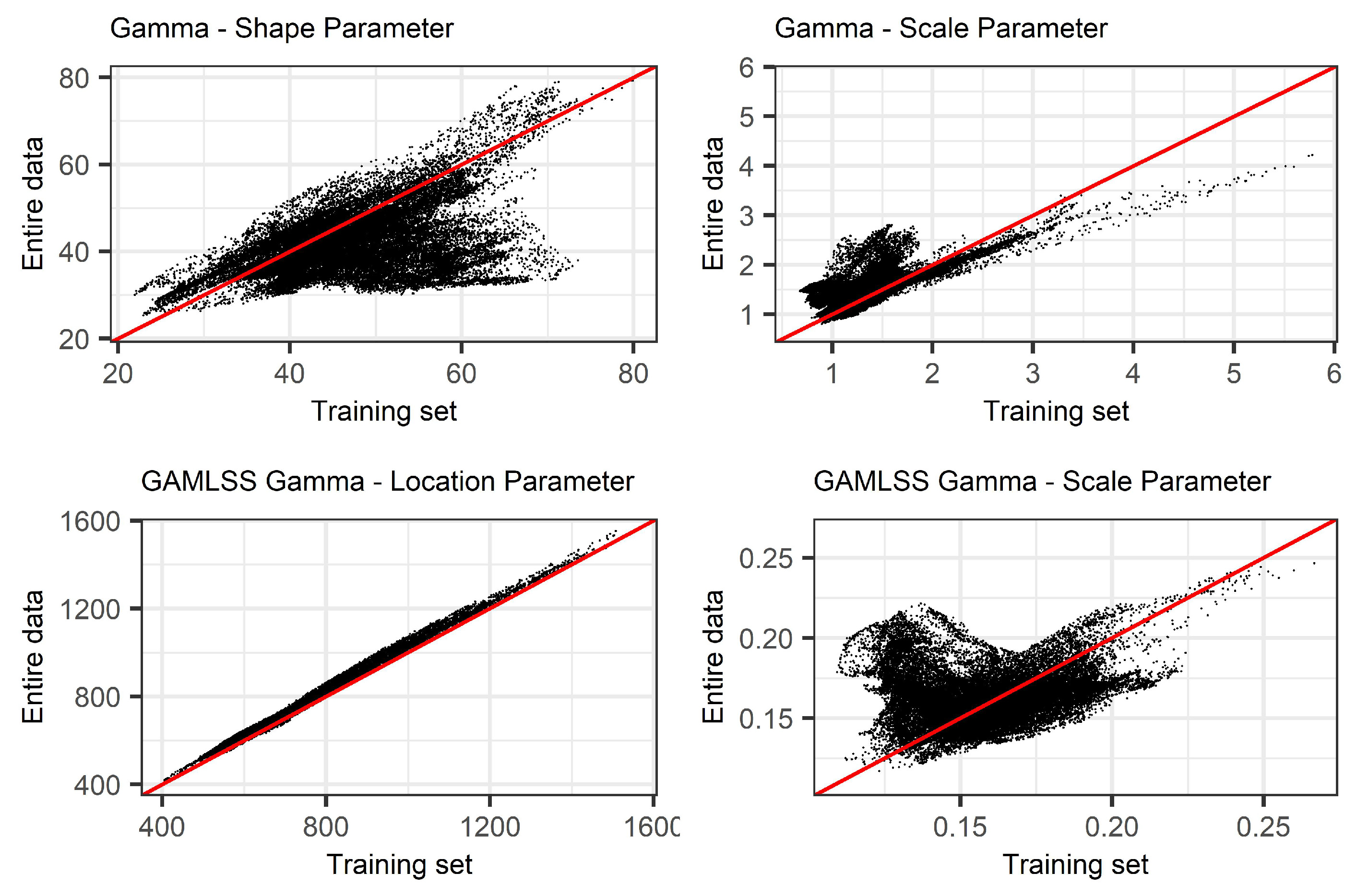
In Section 2.2, we provided the theoretical implications that arise during model-validation when SPI is computed using the entire data. Here, we identify the presence of bias by comparing the parameter estimates of Gamma and non-stationary Gamma distributions using two different subsets of the data and different scales of the index (SPI(3), SPI(6), SPI(9), SPI(12), and SPI(24)). Initially, we fitted the Gamma and non-stationary Gamma distributions on the accumulated precipitation records using the training data, and as a subsequent step, we fitted the same distributions using the training, validation, and test data. Figure 5, provides a graphical comparison of SPI(12) between the parameter estimates of (x-axis) and (y-axis) across the 36,662 basins.
As presented in Figure 5 (top), results show the deviation of the shape and scale parameter estimates from the diagonal. This is an indication of systematic bias in the training data when is compared to . The increased shape parameter in the training set, using , leads to more symmetric shapes (71.1% of the basins have increased shape parameter in the training data). Additionally, the increased scale parameter in the entire data, using , suggests that the distribution of accumulated precipitation has “heavier” tails and consequently higher variance compared to the Gamma distribution fitted on the training data, (76.2% of the basins have increased scale in the entire data). There are two main reasons behind the deviations observed in the parameter estimates: (1) the stationary SPI is time invariant; it uses a location specific Gamma distribution and results in a trending SPI that reflects the same trend as the increasing rainfall trend in Sweden during the last three decades; and (2) the rainfall trend is increasing even further in the validation and test data and this introduces even larger deviations between the parameter estimates of and . In the small scales of the index, the deviations between the parameter estimates present smaller deviations; this is mainly attributed to the short “memory” property of SPI that shares the same parameters with series of shorter length in the validation and test set (Figure 5).
Furthermore, the results from the implementation of NSPI indicate that the location and scale parameter estimates deviate from the diagonal as well (Figure 5, bottom). GAMLSS are able to estimate time-varying location and scale distribution parameters as a function of the increasing trend of accumulated precipitation. However, they are not able to capture the change in distribution of accumulated precipitation in the validation and test sets.
4.2. Drought Class Transitions
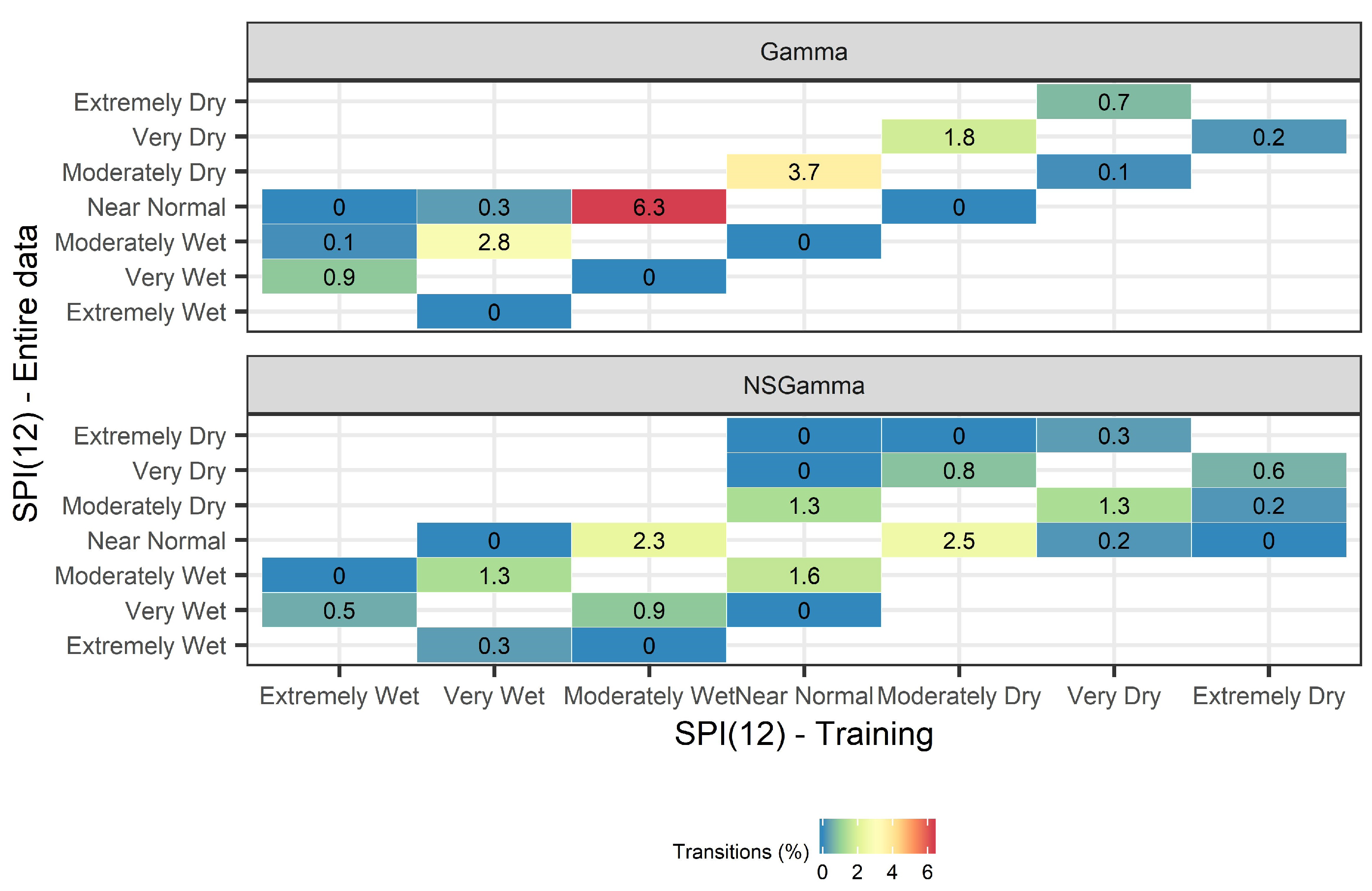
Here, we address the question “Are there drought class transitions in the training set?”. Both the Gamma and NSGamma probability densities were used at different SPI scales (i.e., SPI(3), SPI(6), SPI(9), SPI(12), and SPI(24)) to measure the number of drought classes that change state in the training set when the two different versions of SPI are computed ( versus ). Figure 6 presents the class-transitions in the training set, when either SPI(12) or NSPI(12) is computed using the two aforementioned approaches. The drought class transitions were computed for all 36,662 basins; each basin has available 693 monthly records, leading to 25,406,766 precipitation records in total that were analyzed for this experiment.
Results using both SPI and NSPI are subject to biases in the training data, leading to transitions of drought events when they are calculated using the entire dataset. The computation of a stationary SPI leads to a systematic underestimation of wet events when the index is computed using the entire dataset, i.e., . The most frequent transitions are from Moderately Wet to Near Normal (change at 6.3% of the SPI values, which are 931,968 out of 25,406,766 values) and from Near Normal to Moderately Dry (change at 3.7% of the SPI values). In addition, outliers are observed, where Very Dry events switch to Extremely Dry (change at 0.7% of the SPI values). This systematic change is associated to the increase in the mean monthly precipitation amount in the country during the last three decades, that is not captured through the stationary SPI calculation. This observed increase in precipitation is probably attributed to climate change [43], which is consequently propagated in the SPI estimation and therefore drives the SPI performance. These findings reflect the difference between the monthly precipitation distribution in the training set and the training, validation, and test set. The mean monthly precipitation across all 36,662 basins is equal to 59 mm in the training set (1961–1995) and 64 mm in the validation (1995–2007) and test sets (2007–2018). The systematic trends in drought class transitions (upper triangular in Figure 6) is caused by the stationary nature of SPI and the incorrect computation of index that uses the entire dataset.
NSPI leads to a systematic overestimation and underestimation of drought events in the training data when the index is computed using the entire dataset, i.e., . The most frequent transitions are from Moderately Dry to Near Normal (change at 2.5% of the NSPI values) and from Moderately Wet to Normal (change at 2.3% of the NSPI values) (see Figure 6 NSGamma). Although NSPI involves the calculation of time-varying location and scale distribution parameters in the training set, it is unable to capture the change in the distribution of accumulated precipitation in the validation and test sets, consequently leading to systematic change in the classification of drought events.
4.3. Comparison between the Raw SPI Data
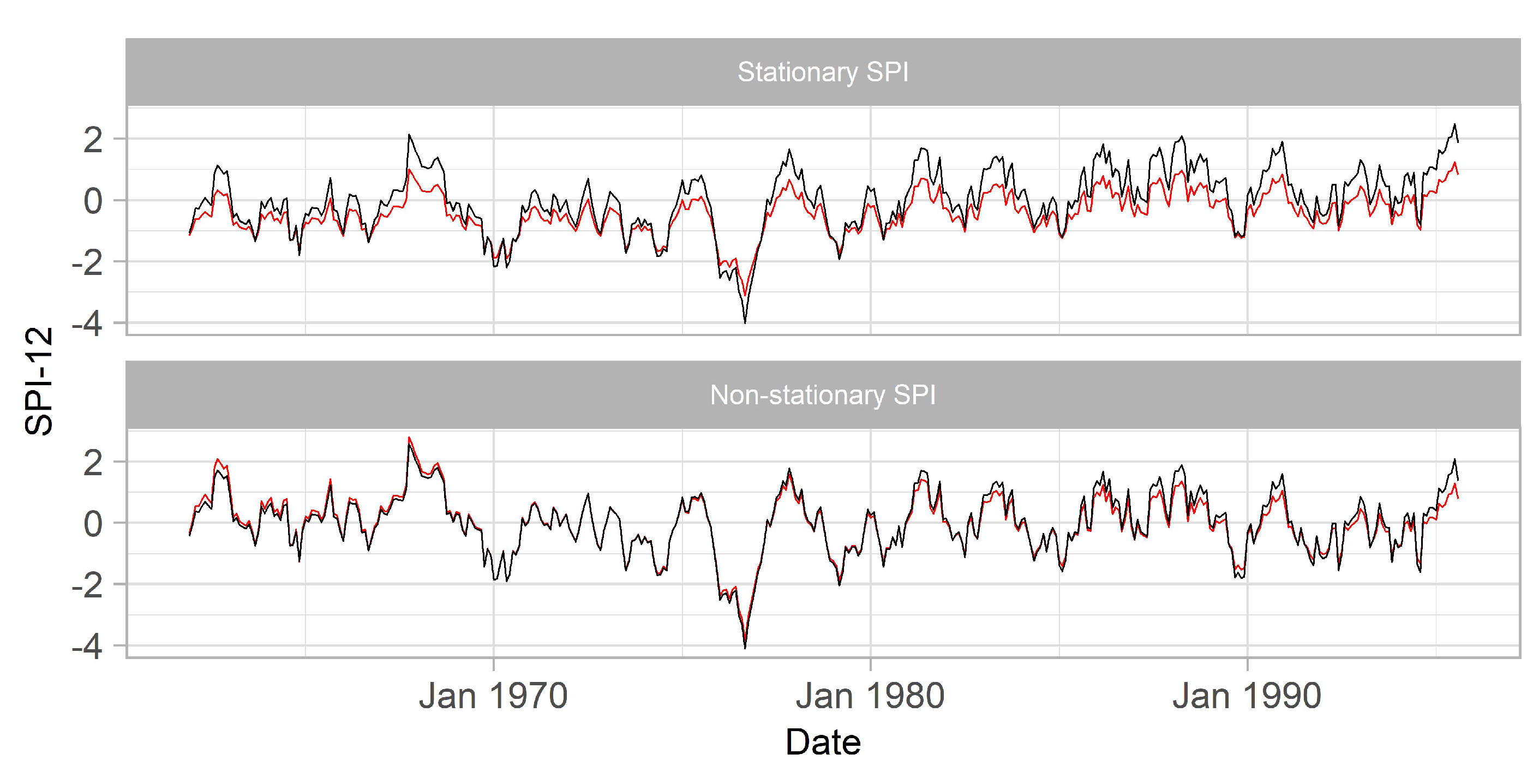
Further analysis on the SPI data provides more in depth diagnostics regarding the effect of the information leakage (bias) in the training set. In Figure 7, SPI and NSPI were calculated using the two computational approaches presented in Section 2.3 for the station S-3357. The stationary SPI, , shows systematically lower values in the training set compared to , consequently leading to more dry events than could have been predicted with the latter approach. This finding is associated to the observed change in the mean monthly precipitation in the validation and test sets which is equal to 94.2 mm, as opposed to to the mean monthly precipitation in the training set which is equal to 77.6 mm. NSPI generates biases of lower magnitude when is compared to (see Figure 7 bottom). This is mainly due to the property of NSPI to capture the increasing precipitation trend and incorporate it in the NSPI calculation, resulting to a trend-free index. The observed deviations between the two NSPI computational approaches are mainly due to the change in the distribution of accumulated precipitation in the validation and test sets that is not captured in the NSPI calculation.
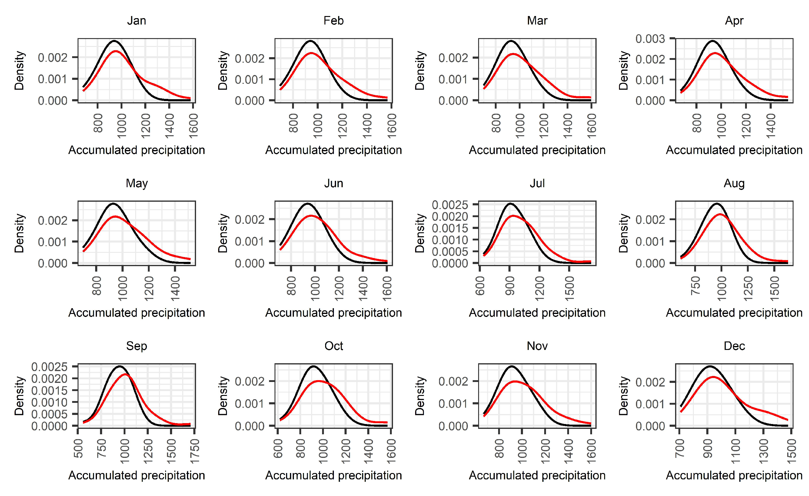
In addition, we investigated whether the observed changes in the raw SPI records for station S-3357 are associated to potential deviations between the distributions of accumulated precipitation in the training and the training, validation, and test sets. In Figure 8, we estimated the density of the 12-month accumulated precipitation for each month. It is clear from the results that the density estimation using the entire data is more skewed to the left compared to the density fitted on the training data, and this is an indication that the variance of accumulated precipitation in the train, validation, and test set is higher than for the entire data.
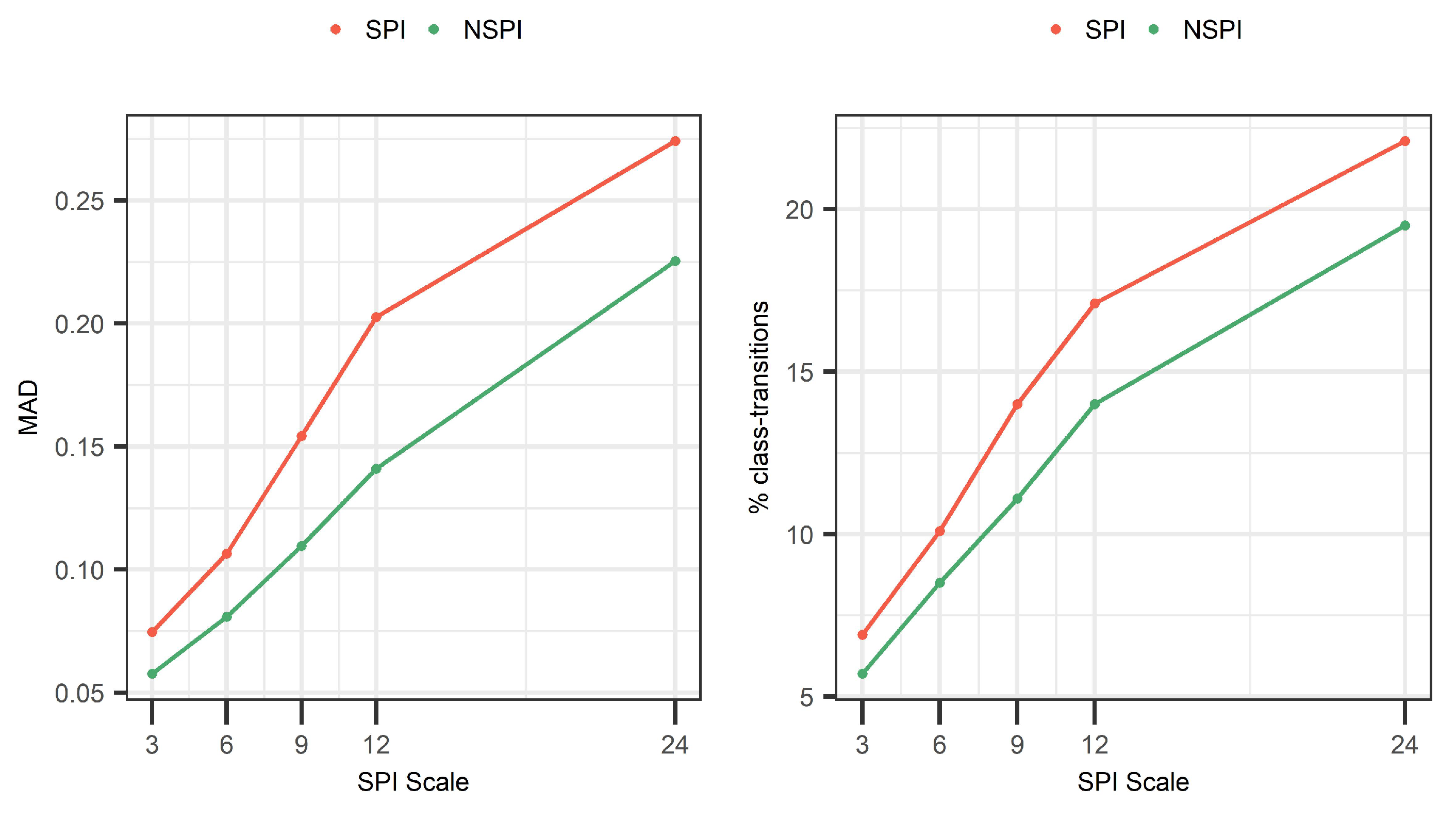
4.4. Sensitivity Analysis of the Bias at Different SPI Scales
We next address the question “Is the bias introduced to the training set sensitive to the SPI scale?” For this, we analyze the bias introduced to the training set at different SPI and NSPI scales (i.e., 3, 6, 9, 12, 24). Results show a positive correlation between the scale of the index and the information leakage in the training set (see Figure 9). In particular, results show that between 6.7% (for SPI(3)) and 22.1% (for SPI(24)) of the training records change drought class, corresponding to deviations (in terms of MAD) between 0.07 and 0.27. The same behavior is observed when different scales of NSPI are calculated, affecting between 5.7% (for NSPI(3)) and 19.3% (for NSPI(24)) of the training records corresponding to deviations (in terms of MAD) between 0.06 and 0.22. This observed dependency of the error to the (N)SPI scale is mainly attributed to the fact that in large scales, the index has long memory and accesses long sequences of the data in the validation and test sets. This finding is in agreement with the results of Wu et al. [30], where larger deviations between the probability density functions were observed in larger accumulated periods.
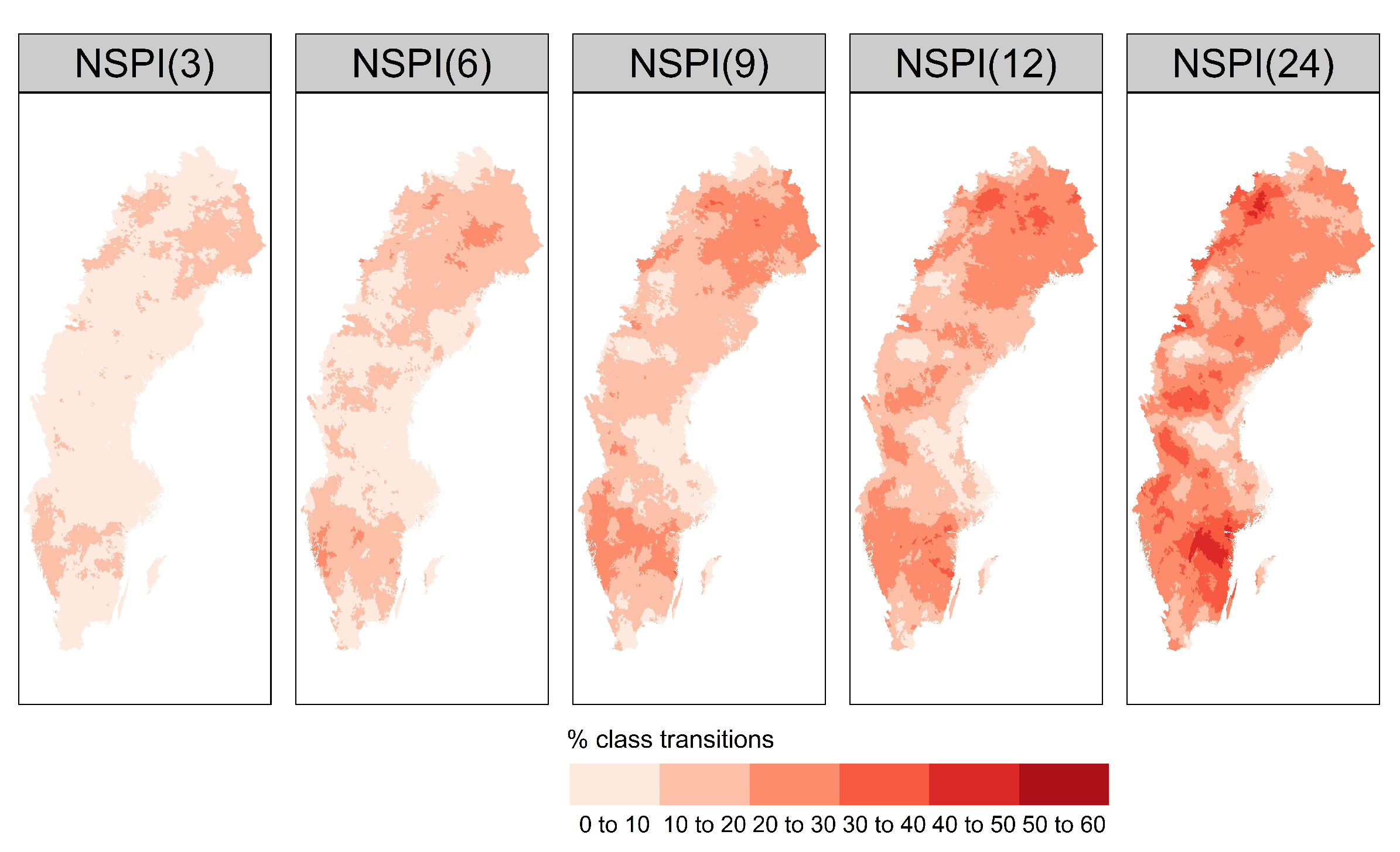
4.5. Bias along a Spatial Gradient
Here, we explore the potential relationship between the bias introduced to the training data and the regional climatic conditions. In this section, we computed the percentage of drought events that change class following the methodology described in Section 2.3.2, and generated the spatial distribution of drought class transitions across the country for different time scales of NSPI (see Figure 10). The percentage of drought class transitions increases with increased NSPI scale and affects up to almost 60% of drought events for certain stations in the southern (snow climate) and northwest part of the country. This result is strongly emphasised at scales NSPI(12) and NSPI(24).
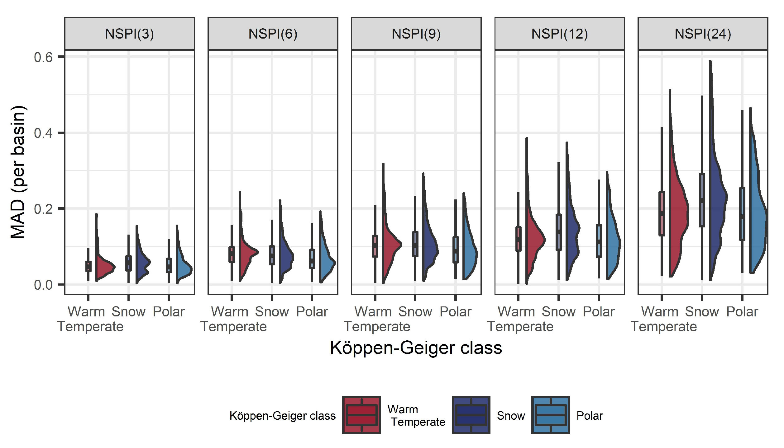
Additionally, the distribution of bias (in terms of MAD) for all 36,662 stations was computed for different time scales and under different climatic conditions. Results in Figure 11 show that the bias increases with increased NSPI scale, while larger deviations are observed in scales NSPI(12) and NSPI(24) and for the snow climatic conditions. This could be attributed to the increase in the mean monthly precipitation during the last decades, however, there might be additional factors, not explicitly addressed in this study, that influence the information leakage issue, such as the physiographic characteristics of the region that could possibly affect the drought spatial variability and its corresponding impacts [44,45].
5. Discussion
5.1. Generalization over a Stronger Spatial Gradient
The results here indicate that change in the climate can be a significant source of bias affecting the training data and, consequently, the learning algorithms that generate drought forecasts. The systematic increase in the mean monthly precipitation in Sweden during the last decades, leads the stationary SPI to underestimate wet events and overestimate dry events in the training set and this is mainly due to the difference in the parameter of the Gamma distribution during estimation (see Figure 5). Similarly, the change in the distribution of accumulated precipitation during the last decades, leads the non-stationary SPI to both overestimate and underestimate wet events. In Europe, the meteorological droughts are associated to decrease in precipitation, especially during the summer period. This precipitation reduction tends to be more severe in the Mediterranean countries that present a different drought regime compared to the rest of Europe [46,47]. Over the next decades, it is projected that temperature will increase more in Europe compared to the global average [48]. A large fraction of Europe is expected to face an increase in the mean temperature of more than 1 C both during winter and summer. With increased warming, winter precipitation is projected to increase with more frequent precipitation in North Eastern Europe, while in South Eastern Europe, precipitation during summer is expected to decrease.
Under these scenarios, there is a clear indication that the precipitation distribution will change over the next decades in Europe. The learning models that will be used to forecast future droughts will be influenced by the potential misuse of the drought indices and will induce bias in the prediction of future drought events. Based on the insights drawn here, it is expected that the bias in the North Eastern part of Europe will lead to overestimation of dry events in the training set, while in the South Eastern Europe it will lead to an underestimation of dry events, when the stationary SPI is employed. Equivalently, changes in the distribution of accumulated precipitation will lead to biases in the training set during NSPI calculation. To prevent this behavior from future drought forecasting applications, we highlight the need to introduce a drought forecasting framework that deals with these limitations and ensures model generalization capability, especially in areas with extreme climatic conditions, i.e., the Mediterranean.
5.2. Applicability Using Different Drought Indices
Although this study focuses on the identification of bias during model-validation using SPI and NSPI, the methodology is valid to other indices whose calculation is performed similarly. For instance, the standardized precipitation-evapotranspiration index (SPEI) [49] and the effective drought index (EDI) [50] have been used thoroughly to also describe the meteorological droughts [51,52]. Additionally, the Palmer severity drought index (PDSI) [53] and the combined drought indicator (CDI) developed by the European Drought Observatory of the Copernicus Emergency Management Service [54] have been used to characterize agricultural droughts [55,56]. Additionally, characterization of hydrological droughts using streamflow information plays a very important role in drought early warning systems, with the most common indices being the variable threshold (VT), the fixed threshold (FT) and the standardized streamflow index (SSI) [57]. The computation of those indices requires attention, particularly since such indices are widely used in climate services and their misuse could lead to incorrect characterization of drought events and incorrect identification of mitigation and adaptation measures.
6. Conclusions
Herein, we highlighted the importance of correct computation of SPI and NSPI in a drought forecasting setting, and demonstrated the theoretical and numerical implications when the index is computed on the entire dataset, which methodologically neglects model-validation. We quantified the bias introduced to the training set by conducting various experiments for different (N)SPI scales from 3 up to 24 months across 36,662 basins in Sweden. Two different computational approaches were compared. First, the SPI and NSPI were computed using the training data only (baseline) and second the SPI and NSPI were computed using the training validation and test data (entire dataset). The latter approach is the one that introduces bias in the training set, as it violates the fundamental principles of OOS model-validation. The main conclusions from this study are as follows:
- Climate change coupled with the computation of SPI prior to model-validation can be a significant source of bias in drought forecasting applications. In the case study presented, the increased precipitation during the last decades leads to changes in the distribution parameters of accumulated precipitation for different time scales of the stationary SPI. This phenomenon affects the estimation of drought in the training set and violates the fundamental principles of OOS model-validation;
- NSPI calculation using GAMLSS, involves the estimation of time-varying location and scale parameters of a Gamma distribution as a function of the increasing trend of accumulated precipitation over time. Although this property results to a trend-free index, still the misuse of the data, introduces biases to the training set;
- The bias introduced to the training data is larger when the stationary SPI is computed. This is mainly because SPI requires fitting the accumulated precipitation records to a time invariant probability density function that incorporates the increasing rainfall trend during SPI calculation. This property leads to a systematic underestimation of wet events in the training data consequently affecting future use of this data in forecasting applications;
- With increased SPI scale, the number of drought class transitions increases and affects up to 22.1% for SPI(24) and 19.3% for NSPI(24) of the available records. This finding is further supported by the MAD metric that indicates increased information leakage with larger SPI and NSPI scales. This is mainly due to the “memory” of the index to access longer sequences of future records during OOS model-validation, thus, leading to increased information leakage issue in the training data;
- The bias introduced due to the incorrect computation of NSPI has spatial dependence, especially in the large scales of the index. The regions affected most are located in the southern (snow climate) and northwest part of the Sweden that exhibit changes in the distribution of accumulated precipitation in the validation and test sets.
Taking into account the findings presented in this paper, we propose that many existing drought forecasting studies that focus on the prediction of SPI should not be applied to real world forecasting applications if the fundamental principles of OOS model-validation are violated. It is expected that the bias introduced to the training set can have a significant impact on the learning algorithms under the drought forecasting setting, especially in larger scales of the index and varying climatic conditions. Even though, the results presented are related to the climatic conditions of Sweden, they could be directly applied to other climatic regions that stronger changes in precipitation have been recorded, i.e., the Mediterranean. It is expected that the bias identified here would be substantial in such climates, and consequently significantly affect the drought predictions and corresponding decision-making.
Author Contributions
Conceptualization, K.M. and D.F.L.; methodology, K.M.; software, K.M.; validation, K.M.; formal analysis, K.M.; investigation, K.M. and D.F.L.; resources, K.M.; data curation, K.M.; writing—original draft preparation, K.M.; writing—review and editing, K.M. and D.F.L.; visualization, K.M.; supervision, D.F.L. All authors have read and agreed to the published version of the manuscript.
Funding
Not applicable.
Institutional Review Board Statement
Not applicable.
Informed Consent Statement
Not applicable.
Data Availability Statement
The meteorological data used for driving the investigation are available from the luftweb portal (https://luftweb.smhi.se, accessed on January 2020), and the vattenweb portal (https://www.smhi.se/data/hydrologi/vattenwebb, accessed on 1 January 2020). The code base of the experiments can be found in a Github repository: https://github.com/mammask/droughtBias, accessed on 9 September 2021.
Acknowledgments
The authors would like to thank Niclas Hjerdt and Ilias G. Pechlivanidis for giving permission to use the data in this investigation.
Conflicts of Interest
The authors declare no conflict of interest.
Appendix A. Stationary Standardized Precipitation Index
The standardized precipitation index (SPI), proposed by [4], defines and monitors drought events. Positive SPI values indicate wet conditions with greater than the median precipitation, while negative SPI values indicate dry conditions with lower than the median precipitation. Table A1 provides the classification of different SPI values.

Table A1.
SPI ranges for different meteorological conditions.
| SPI Values | Classification |
|---|---|
| Extremely Wet | |
| Very Wet | |
| Moderately Wet | |
| Near Normal | |
| Moderately Dry | |
| Very Dry | |
| Extremely Dry |
The computation of SPI requires fitting a probability distribution on monthly aggregated precipitation series at different time scales (e.g., 3, 6, 9, 12 months). Usually, the Gamma distribution fits best precipitation data and is given by the following expression:
for where is the shape parameter, is the scale parameter and x is the precipitation amount. The Gamma function is defined by the integral:
Fitting the Gamma distribution to the monthly precipitation records requires the estimation of the and parameters using maximum likelihood estimation [58].
where:
and n is the number of precipitation records. The resulting parameters are used to compute the cumulative probability of the observed precipitation records for a given period and time scale [58].
The Gamma distribution is undefined for since there may be no precipitation and by letting [58] the incomplete Gamma distribution is given by:
Appendix B. Non-Stationary Standardized Precipitation Index (NSPI)
In this study, we computed the non-stationary version of SPI (NSPI) using the GAMLSS framework introduced by Rigby and Stasinopoulos [59]. GAMLSS has been thoroughly used in the past to model non-stationary versions of drought indices [60,61]. It is a semi-parametric regression model, in which a parametric distribution assumption is required for the response variable, and the selected distribution’s parameters can vary as a function of explanatory variables or random effects. Within the GAMLSS framework, observations , for , where n is the length of the observations, are assumed to be independent and fitted to a probability density function , conditional on , where p is the number of distribution parameters at time t. Various distributions are supported by GAMLSS, including, highly skew or kurtotic continuous and discrete distributions. The distribution parameters , characterized as location, shape, and scale parameters are related to explanatory variables by monotonic link functions , , given by:
where and are vectors of length n, , is a parameter vector of length , is a fixed known design matrix of order , is a fixed known design matrix, and is a dimensional random variable. In Equation (A8), for , , are comprised of a parametric component (functions of explanatory variables) and additive components (random effects). If , the model is reduced to a fully parametric GAMLSS model.
Here, we computed NSPI by fitting a GAMLSS on the accumulated precipitation series using different time scales. The accumulated precipitation series were assumed to follow a two-parameter Gamma distribution with its location and scale parameters, linked to a linear trend that evolves over time, t. The following additive formulation was used in this study:
where and are the location and scale parameters of the Gamma distribution with the link functions and , respectively. is a matrix of covariates (in our case a linear trend that evolves over time) of order , , is a parameter vector of length , and represents the dependence function of the distribution parameters on the linear trend . Mathematically, NSPI is similar to SPI, because they have similar calculation steps, however, NSPI is based on a non-stationary Gamma with time-varying location and scale parameters.
Appendix C. Comparison of Distribution Parameters
Figure A1.
(top) Comparison between the stationary Gamma distribution parameter estimates (SPI); (bottom) Aggregated GAMLSS location and scale parameters of non-stationary Gamma (NSPI) of accumulated precipitation between (y-axis) and (x-axis) for 36,662 basins in Sweden during 1961–2018.
Figure A1.
(top) Comparison between the stationary Gamma distribution parameter estimates (SPI); (bottom) Aggregated GAMLSS location and scale parameters of non-stationary Gamma (NSPI) of accumulated precipitation between (y-axis) and (x-axis) for 36,662 basins in Sweden during 1961–2018.

References
- FAO. The Impact of Disasters on Agriculture and Food Security; Technical Report; Food and Agriculture Organization of the United Nations: Rome, Italy, 2015. [Google Scholar]
- Cammalleri, C.; Naumann, G.; Mentaschi, L.; Formetta, G.; Forzieri, G.; Gosling, S.; Bisselink, B.; De Roo, A.; Feyen, L. Global Warming and Drought Impacts in the EU; Joint Research Centre (JRC): Brussels, Belgium, 2020. [Google Scholar]
- Vogt, J.; Sepulcre, G.; Magni, D.; Valentini, L.; Singleton, A.; Micale, F.; Barbosa, P. The European Drought Observatory (EDO): Current State and Future Directions; EGU General Assembly: Vienna, Austria, 2013; p. EGU2013-7374. [Google Scholar]
- McKee, T.B.; Doesken, N.J.; Kleist, J. The relationship of drought frequency and duration to time scales. In Proceedings of the 8th Conference on Applied Climatology, Anaheim, CA, USA, 17–22 January 1993; Volume 17, pp. 179–183. [Google Scholar]
- Hao, Z.; AghaKouchak, A.; Nakhjiri, N.; Farahmand, A. Global integrated drought monitoring and prediction system. Sci. Data 2014, 1, 1–10. [Google Scholar] [CrossRef]
- Sutanto, S.J.; Van Lanen, H.A.; Wetterhall, F.; Llort, X. Potential of pan-european seasonal hydrometeorological drought forecasts obtained from a multihazard early warning system. Bull. Am. Meteorol. Soc. 2020, 101, E368–E393. [Google Scholar] [CrossRef] [Green Version]
- Tsakiris, G.; Vangelis, H. Towards a drought watch system based on spatial SPI. Water Resour. Manag. 2004, 18, 1–12. [Google Scholar] [CrossRef]
- Livada, I.; Assimakopoulos, V. Spatial and temporal analysis of drought in Greece using the Standardized Precipitation Index (SPI). Theor. Appl. Climatol. 2007, 89, 143–153. [Google Scholar] [CrossRef]
- Patel, N.R.; Chopra, P.; Dadhwal, V.K. Analyzing spatial patterns of meteorological drought using standardized precipitation index. Meteorol. Appl. 2007, 14, 329–336. [Google Scholar] [CrossRef]
- Karavitis, C.; Alexandris, S.; Tsesmelis, D.; Athanasopoulos, G. Application of the standardized precipitation index (SPI) in Greece. Water 2011, 3, 787–805. [Google Scholar] [CrossRef]
- Van Loon, A.F.; Tijdeman, E.; Wanders, N.; Van Lanen, H.J.; Teuling, A.; Uijlenhoet, R. How climate seasonality modifies drought duration and deficit. J. Geophys. Res. Atmos. 2014, 119, 4640–4656. [Google Scholar] [CrossRef]
- Guenang, G.M.; Kamga, F.M. Computation of the standardized precipitation index (SPI) and its use to assess drought occurrences in Cameroon over recent decades. J. Appl. Meteorol. Climatol. 2014, 53, 2310–2324. [Google Scholar] [CrossRef]
- Wang, H.; Chen, Y.; Pan, Y.; Chen, Z.; Ren, Z. Assessment of candidate distributions for SPI/SPEI and sensitivity of drought to climatic variables in China. Int. J. Climatol. 2019, 39, 4392–4412. [Google Scholar] [CrossRef]
- Stagge, J.H.; Tallaksen, L.M.; Gudmundsson, L.; Van Loon, A.F.; Stahl, K. Candidate distributions for climatological drought indices (SPI and SPEI). Int. J. Climatol. 2015, 35, 4027–4040. [Google Scholar] [CrossRef]
- Angelidis, P.; Maris, F.; Kotsovinos, N.; Hrissanthou, V. Computation of drought index SPI with alternative distribution functions. Water Resour. Manag. 2012, 26, 2453–2473. [Google Scholar] [CrossRef]
- Sienz, F.; Bothe, O.; Fraedrich, K. Monitoring and quantifying future climate projections of dryness and wetness extremes: SPI bias. Hydrol. Earth Syst. Sci. 2012, 16, 2143–2157. [Google Scholar] [CrossRef] [Green Version]
- Alam, N.; Raizada, A.; Jana, C.; Meshram, R.K.; Sharma, N. Statistical modeling of extreme drought occurrence in Bellary District of Eastern Karnataka. Proc. Natl. Acad. Sci. India Sect. B Biol. Sci. 2015, 85, 423–430. [Google Scholar] [CrossRef]
- Shiau, J.T. Effects of gamma-distribution variations on SPI-based stationary and nonstationary drought analyses. Water Resour. Manag. 2020, 34, 2081–2095. [Google Scholar] [CrossRef]
- Russo, S.; Dosio, A.; Sterl, A.; Barbosa, P.; Vogt, J. Projection of occurrence of extreme dry-wet years and seasons in Europe with stationary and nonstationary Standardized Precipitation Indices. J. Geophys. Res. Atmos. 2013, 118, 7628–7639. [Google Scholar] [CrossRef] [Green Version]
- Wang, Y.; Li, J.; Feng, P.; Hu, R. A time-dependent drought index for non-stationary precipitation series. Water Resour. Manag. 2015, 29, 5631–5647. [Google Scholar] [CrossRef]
- Box, G.; Jenkins, E.M. Time Series Analysis: Forecasting and Control; Holden-Day, Inc.: San Francisco, CA, USA, 1970. [Google Scholar]
- Mishra, A.K.; Desai, V.R. Drought forecasting using stochastic models. Stoch. Environ. Res. Risk Assess 2005, 19, 326–339. [Google Scholar] [CrossRef]
- Han, P.; Wang, P.; Tian, M.; Zhang, S.; Liu, J.; Zhu, D. Application of the ARIMA models in drought forecasting using the standardized precipitation index. IFIP Adv. Inf. Commun. Technol. 2013, 392, 352–358. [Google Scholar] [CrossRef] [Green Version]
- Yeh, H.F.; Hsu, H.L. Stochastic model for drought forecasting in the southern Taiwan basin. Water 2019, 11, 2041. [Google Scholar] [CrossRef] [Green Version]
- Sutanto, S.J.; Wetterhall, F.; Van Lanen, H.A. Hydrological drought forecasts outperform meteorological drought forecasts. Environ. Res. Lett. 2020, 15, 084010. [Google Scholar] [CrossRef]
- Vapnik, V.; Golowich, S.E.; Smola, A.J. Support Vector Method for Function Approximation, Regression Estimation and Signal Processing. In Proceedings of the NIPS’96 9th International Conference on Neural Information Processing Systems, Denver, CO, USA, 3–5 December 1996; MIT Press: Cambridge, MA, USA, 1996; pp. 281–287. [Google Scholar]
- McCulloch, W.; Pitts, W. A Logical Calculus of Ideas Immanent in Nervous Activity. Bull. Math. Biophys. 1943, 5, 115–133. [Google Scholar] [CrossRef]
- Belayneh, A.; Adamowski, J. Drought forecasting using new machine learning methods. J. Water Land Dev. 2013, 18, 3–12. [Google Scholar] [CrossRef]
- Mokhtarzad, M.; Eskandari, F.; Vanjani, N.J.; Arabasadi, A. Drought forecasting by ANN, ANFIS, and SVM and comparison of the models. Environ. Earth Sci. 2017, 76, 729. [Google Scholar] [CrossRef]
- Wu, H.; Hayes, M.J.; Wilhite, D.A.; Svoboda, M.D. The effect of the length of record on the standardized precipitation index calculation. Int. J. Climatol. 2005, 25, 505–520. [Google Scholar] [CrossRef] [Green Version]
- Rezaeian-Zadeh, M.; Tabari, H. MLP-based drought forecasting in different climatic regions. Theor. Appl. Climatol. 2012, 109, 407–414. [Google Scholar] [CrossRef]
- Belayneh, A.; Adamowski, J.; Khalil, B.; Ozga-Zielinski, B. Long-term SPI drought forecasting in the Awash River Basin in Ethiopia using wavelet neural network and wavelet support vector regression models. J. Hydrol. 2014, 508, 418–429. [Google Scholar] [CrossRef]
- Deo, R.C.; Kisi, O.; Singh, V.P. Drought forecasting in eastern Australia using multivariate adaptive regression spline, least square support vector machine and M5Tree model. Atmos. Res. 2017, 184, 149–175. [Google Scholar] [CrossRef] [Green Version]
- Yaseen, Z.M.; Ali, M.; Sharafati, A.; Al-Ansari, N.; Shahid, S. Forecasting standardized precipitation index using data intelligence models: Regional investigation of Bangladesh. Sci. Rep. 2021, 11, 1–25. [Google Scholar] [CrossRef]
- Rhee, J.; Im, J. Meteorological drought forecasting for ungauged areas based on machine learning: Using long-range climate forecast and remote sensing data. Agric. For. Meteorol. 2017, 237, 105–122. [Google Scholar] [CrossRef]
- Tashman, L.J. Out-of-sample tests of forecasting accuracy: An analysis and review. Int. J. Forecast. 2004, 16, 437–450. [Google Scholar] [CrossRef]
- Bergmeir, C.; Benitez, J.M. On the Use of Cross-validation for Time Series Predictor Evaluation. Inf. Sci. 2012, 191, 192–213. [Google Scholar] [CrossRef]
- Hastie, T.; Tibshirani, R.; Friedman, J. The Elements of Statistical Learning: Prediction, Inference and Data Mining, 2nd ed.; Springer: New York, NY, USA, 2009; pp. 241–260. [Google Scholar]
- Mishra, A.K.; Desai, V.R.; Singh, V.P. Drought forecasting using a hybrid stochastic and neural network model. Hydrol. Eng. ASCE 2007, 12, 626–638. [Google Scholar] [CrossRef]
- Kottek, M.; Grieser, J.; Beck, C.; Rudolf, B.; Rubel, F. World map of the Köppen-Geiger climate classification updated. Hydrol. Earth Syst. Sci 2006. [Google Scholar] [CrossRef]
- Girons Lopez, M.; Crochemore, L.; Pechlivanidis, I.G. Benchmarking an operational hydrological model for providing seasonal forecasts in Sweden. Hydrol. Earth Syst. Sci. 2021, 25, 1189–1209. [Google Scholar] [CrossRef]
- Guide, Svoboda, Hayes, and Wood; World Meteorological Organization: Geneva, Switzerland, 2012.
- Arheimer, B.; Lindström, G. Climate impact on floods: Changes in high flows in Sweden in the past and the future (1911–2100). Hydrol. Earth Syst. Sci. 2015, 19, 771–784. [Google Scholar] [CrossRef] [Green Version]
- Van Loon, A.; Van Huijgevoort, M.; Van Lanen, H. Evaluation of drought propagation in an ensemble mean of large-scale hydrological models. Hydrol. Earth Syst. Sci. 2012, 16, 4057–4078. [Google Scholar] [CrossRef] [Green Version]
- Van Loon, A.; Laaha, G. Hydrological drought severity explained by climate and catchment characteristics. J. Hydrol. 2015, 526, 3–14. [Google Scholar] [CrossRef] [Green Version]
- Blauhut, V.; Stahl, K.; Stagge, J.; Tallaksen, L.; De Stefano, L.; Vogt, J. Estimating drought risk across Europe from reported drought impacts, drought indices, and vulnerability factor. Hydrol. Earth Syst. Sci. 2016, 20, 2779–2800. [Google Scholar] [CrossRef] [Green Version]
- Hanel, M.; Rakovec, O.; Markonis, Y.; Maca, P.; Samaniego, L.; Kysely, J.; Kumar, R. Revisiting the recent European droughts from a long-term perspective. Sci. Rep. 2018, 8, 1–11. [Google Scholar] [CrossRef] [PubMed]
- Dosio, A. Mean and Extreme Climate in Europe under 1.5, 2, and 3 °C Global Warming; JRC PESETA IV Project—Task 1; Publications Office of the European Union: Luxembourg, 2020. [Google Scholar] [CrossRef]
- Vicente-Serrano, S.M.; Beguería, S.; Lopez-Moreno, J.I. A multiscalar drought index sensitive to global warming: The standardized precipitation evapotranspiration index. Water Resour. Manag. 2010, 23, 1696–1718. [Google Scholar] [CrossRef] [Green Version]
- Byun, H.R.; Wilhite, D.A. Objective quantification of drought severity and duration. J. Clim. 1999, 12, 2747–2756. [Google Scholar] [CrossRef]
- Beguería, S.; Vicente-Serrano, S.M.; Reig, F.; Latorre, B. Standardized precipitation evapotranspiration index (SPEI) revisited: Parameter fitting, evapotranspiration models, tools, datasets and drought monitoring. Int. J. Climatol. 2014, 34, 3001–3023. [Google Scholar] [CrossRef] [Green Version]
- Deo, R.C.; Byun, H.R.; Adamowski, J.F.; Begum, K. Application of effective drought index for quantification of meteorological drought events: A case study in Australia. Theor. Appl. Climatol. 2017, 128, 359–379. [Google Scholar] [CrossRef]
- Palmer, W.C. Meteorological Drought; US Department of Commerce, Weather Bureau: Silver Spring, MD, USA, 1965; Volume 30.
- Sepulcre-Canto, G.; Horion, S.; Singleton, A.; Carrao, H.; Vogt, J. Development of a Combined Drought Indicator to detect agricultural drought in Europe. Nat. Hazards Earth Syst. Sci. 2012, 12, 3519–3531. [Google Scholar] [CrossRef] [Green Version]
- Vicente-Serrano, S.M.; Beguería, S.; López-Moreno, J.I. Comment on “Characteristics and trends in various forms of the Palmer Drought Severity Index (PDSI) during 1900–2008” by Aiguo Dai. J. Geophys. Res. Atmos. 2011, 116. [Google Scholar] [CrossRef] [Green Version]
- Balint, Z.; Mutua, F.; Muchiri, P.; Omuto, C.T. Monitoring drought with the combined drought index in Kenya. In Developments in Earth Surface Processes; Elsevier: Amsterdam, The Netherlands, 2013; Volume 16, pp. 341–356. [Google Scholar]
- Sutanto, S.J.; Van Lanen, H.A. Streamflow drought: Implication of drought definitions and its application for drought forecasting. Hydrol. Earth Syst. Sci. Discuss. 2021, 25, 3991–4023. [Google Scholar] [CrossRef]
- Thom, H.C.S. A note on gamma distribution. Mon. Weather Rev. 1958, 86, 117–122. [Google Scholar] [CrossRef]
- Rigby, R.A.; Stasinopoulos, D.M. Generalized additive models for location, scale and shape. J. R. Stat. Soc. Ser. C (Appl. Stat.) 2005, 54, 507–554. [Google Scholar] [CrossRef] [Green Version]
- Villarini, G.; Smith, J.A.; Napolitano, F. Nonstationary modeling of a long record of rainfall and temperature over Rome. Adv. Water Resour. 2010, 33, 1256–1267. [Google Scholar] [CrossRef]
- Bazrafshan, J.; Hejabi, S. A non-stationary reconnaissance drought index (NRDI) for drought monitoring in a changing climate. Water Resour. Manag. 2018, 32, 2611–2624. [Google Scholar] [CrossRef]
Figure 1.
Conceptualization of data separation in model-validation. Training (blue), validation (orange) and test (green) datasets are shown for the OOS, 3-Fold CV and 3-Fold B-CV methods.
Figure 1.
Conceptualization of data separation in model-validation. Training (blue), validation (orange) and test (green) datasets are shown for the OOS, 3-Fold CV and 3-Fold B-CV methods.

Figure 2.
Calculation of the SPI using different subsets of the data within time series cross-validation.
Figure 2.
Calculation of the SPI using different subsets of the data within time series cross-validation.

Figure 3.
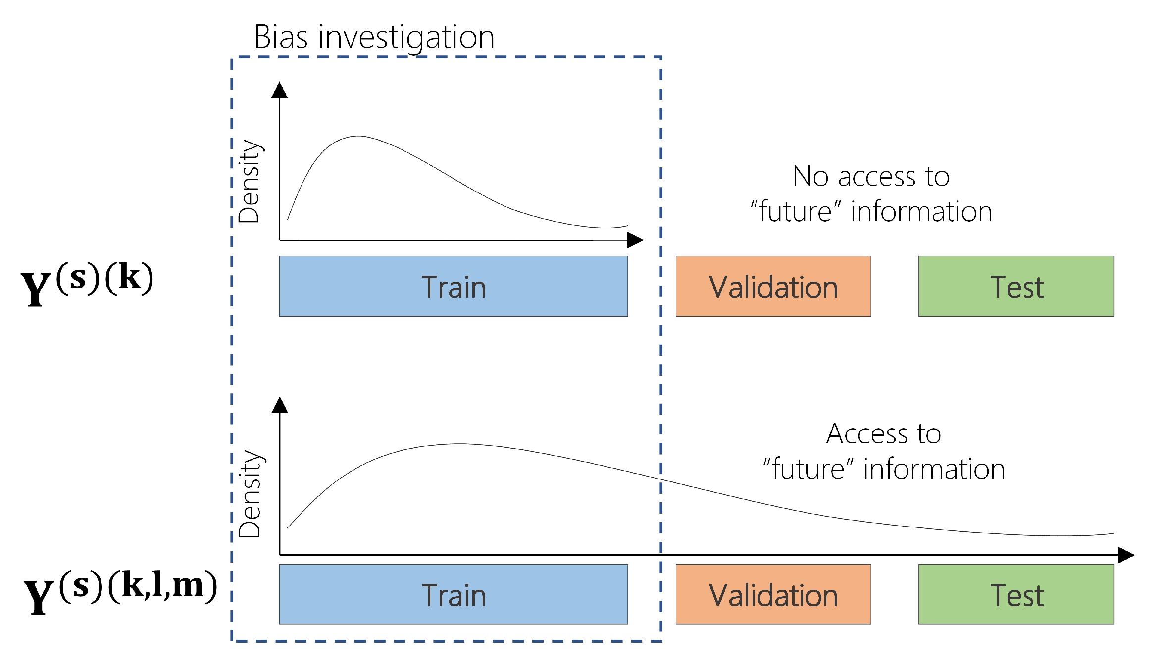
Two computational approaches of (N)SPI calculation. (top) (N)SPI calculation using the training set (), (bottom) (N)SPI calculation using the training, validation and test sets ().
Figure 3.
Two computational approaches of (N)SPI calculation. (top) (N)SPI calculation using the training set (), (bottom) (N)SPI calculation using the training, validation and test sets ().

Figure 4.
(left) Locations of precipitation stations used over Sweden. (center) Spatial distribution of the Köppen-Geiger climate classification system. (right) Mean monthly precipitation (mm) during the period 1961–2018.
Figure 4.
(left) Locations of precipitation stations used over Sweden. (center) Spatial distribution of the Köppen-Geiger climate classification system. (right) Mean monthly precipitation (mm) during the period 1961–2018.

Figure 5.
Comparison between the distribution parameter estimates of accumulated precipitation between (y-axis) and (x-axis) for 36,662 basins in Sweden during 1961–2018: (top) stationary SPI and (bottom) non-stationary SPI.
Figure 5.
Comparison between the distribution parameter estimates of accumulated precipitation between (y-axis) and (x-axis) for 36,662 basins in Sweden during 1961–2018: (top) stationary SPI and (bottom) non-stationary SPI.

Figure 6.
Transition of drought classes from (x-axis) to (y-axis) for 36,662 basins in Sweden during the period 1961–2018. Blue color leads to changes of lower magnitude while red color leads to changes of higher magnitude.
Figure 6.
Transition of drought classes from (x-axis) to (y-axis) for 36,662 basins in Sweden during the period 1961–2018. Blue color leads to changes of lower magnitude while red color leads to changes of higher magnitude.

Figure 7.
Comparison between (red) and (black) using Gamma and NSGamma probability density functions.
Figure 7.
Comparison between (red) and (black) using Gamma and NSGamma probability density functions.

Figure 8.
Comparison of the density estimates of the accumulated rainfall between (black) and (red).
Figure 8.
Comparison of the density estimates of the accumulated rainfall between (black) and (red).

Figure 9.
Mean absolute deviation (left), percentage of records with drought class transitions (right); for different scales of SPI and NSPI across Sweden.
Figure 9.
Mean absolute deviation (left), percentage of records with drought class transitions (right); for different scales of SPI and NSPI across Sweden.

Figure 10.
Percentage of drought class transitions for different scales of SPI, using the non-stationary Gamma distribution, across 36,662 basins.
Figure 10.
Percentage of drought class transitions for different scales of SPI, using the non-stationary Gamma distribution, across 36,662 basins.

Figure 11.
Distribution of the mean absolute deviation (MAD) between the NSPI computed on the training set only and the NSPI computed on the training, validation and test sets for different Köppen-Geiger climatic classes and 36,662 basins in Sweden during 1961–2018.
Figure 11.
Distribution of the mean absolute deviation (MAD) between the NSPI computed on the training set only and the NSPI computed on the training, validation and test sets for different Köppen-Geiger climatic classes and 36,662 basins in Sweden during 1961–2018.

Table 1.
S-3357 meteorological station.
| Station | Longitude | Latitude | Mean Monthly Rainfall (Train) | Mean Monthly Rainfall (Train, Valid, Test) |
|---|---|---|---|---|
| S-3357 | 67.37 | 22.28 | 77.6 mm | 84.2 mm |
Publisher’s Note: MDPI stays neutral with regard to jurisdictional claims in published maps and institutional affiliations. |
© 2021 by the authors. Licensee MDPI, Basel, Switzerland. This article is an open access article distributed under the terms and conditions of the Creative Commons Attribution (CC BY) license (https://creativecommons.org/licenses/by/4.0/).
Share and Cite
MDPI and ACS Style
Mammas, K.; Lekkas, D.F. Characterization of Bias during Meteorological Drought Calculation in Time Series Out-of-Sample Validation. Water 2021, 13, 2531. https://doi.org/10.3390/w13182531
AMA Style
Mammas K, Lekkas DF. Characterization of Bias during Meteorological Drought Calculation in Time Series Out-of-Sample Validation. Water. 2021; 13(18):2531. https://doi.org/10.3390/w13182531
Chicago/Turabian StyleMammas, Konstantinos, and Demetris F. Lekkas. 2021. "Characterization of Bias during Meteorological Drought Calculation in Time Series Out-of-Sample Validation" Water 13, no. 18: 2531. https://doi.org/10.3390/w13182531
Note that from the first issue of 2016, this journal uses article numbers instead of page numbers. See further details here.