
Numerical Simulations of 2D Hydraulic Jumps by a Parallel SPH Model


1
College of Ocean Engineering, Guangdong Ocean University, Zhanjiang 524088, China
2
School of Marine Engineering Equipment, Zhejiang Ocean University, Zhoushan 316022, China
3
Maritime College, Guangdong Ocean University, Zhanjiang 524088, China
4
State Key Laboratory of Coastal and Offshore Engineering, Dalian University of Technology, Dalian 116024, China
*
Author to whom correspondence should be addressed.
†
These authors contributed equally to this work and should be considered co-first authors.
Water 2021, 13(18), 2536; https://doi.org/10.3390/w13182536
Submission received: 6 July 2021
/
Revised: 23 August 2021
/
Accepted: 25 August 2021
/
Published: 16 September 2021
(This article belongs to the Section Hydraulics and Hydrodynamics)
Abstract
:Hydraulic jumps are a rapid transition from supercritical to subcritical flow and generally occur in rivers or spillways. Owing to the high energy dissipation rate, hydraulic jumps are widely applied as energy dissipators in hydraulic projects. To achieve efficient and accurate simulations of 2D hydraulic jumps in open channels, a parallel Weakly Compressible Smoothed Particle Hydrodynamics model (WCSPH) with Shepard Density filter was established in this study. The acceleration of the model was obtained by OpenMP to reduce execution time. To further reduce execution time, a suitable and efficient scheduling strategy was selected for the parallel numerical model by comparing parallel speed-ups under different scheduling strategies in OpenMP. Following this, two test cases of uniform flow in open channels and hydraulic jumps with different inflow conditions were investigated to validate the model. The comparison of the water depth and velocity fields between the numerical results and the analytical solution generally showed good agreement, although there was a minor discrepancy in conjugate water depths. The numerical results showed free surface undulation with decreasing amplitude, which is more consistent with physical reality, with a low inflow Froude number. Simultaneously, the Shepard filter was able to smooth the pressure fields of the hydraulic jumps with a high inflow Froude number. Moreover, the parallel speed-up was generally able to reach theoretical maximum acceleration by analyzing the performance of the model according to different particle numbers.
1. Introduction
A special hydraulic phenomenon, where the water depth in a short channel jumps sharply from less than the critical depth to greater than the critical depth, will occur when flow in an open channel transitions from subcritical to supercritical. This special hydraulic event is described as the phenomenon of hydraulic jumps. Hydraulic jumps often occur downstream of a sluice, dam, and/or steep groove. Since the consumption of mechanical energy can be massive during the strong friction and mixing of water in hydraulic jumps, hydraulic jumps are usually exploited to dissipate excess energy.
At present, most of the research on hydraulic jumps is based on Eulerian grid-based methods [1,2,3,4]. However, Level Set (LS) or Volume-of-Fluid (VOF) methods were necessary to capture the water surface in the Eulerian grid-based methods, due to the complexity of hydraulic jumps, such as large deformation and rapid change of flow filed. Sometimes, other specific treatments, such as refining the mesh near the bed or jump zone, and reducing the time step, were also needed to reproduce the characteristics of hydraulic jumps. These specific treatments make it difficult and inefficient to solve the Euler model. To overcome these difficulties in numerical simulations, meshless numerical methods have attracted more and more attention from researchers in recent years. Meshless methods are especially suitable for calculations with discontinuous or large deformation-free surfaces, since the calculation of governing equations is based upon a set of discrete particles that can move freely. As a representative meshless method, the Smoothed Particle Hydrodynamics method (SPH) has developed rapidly in recent years and has been widely used for important problems in computational fluid dynamics (CFD), including free surface flow, multiphase flow, wave, non-Newtonian fluid, and so on.
The SPH method has been employed to investigate hydraulic jumps. López, Jonsson, and Gu et al. [5,6,7] separately investigated the feasibility and capability of the SPH model in 2D hydraulic jumps on a flat as well as on a corrugated riverbed. Some inlet and outlet boundary algorithms for the SPH method were developed from the studies. In the SPH method, the boundary algorithms could enforce different upstream/downstream flow conditions and implemented the inlet and outlet boundary setting. The accuracy of the SPH model in computing hydraulic jumps was verified based on comparisons of water elevation, jump-toe position, jump depth, and the pressure on the basin bottom under different viscosity treatments. De Padova et al. [8] investigated three-dimensional undular hydraulic jumps in a large channel by means of an XSPH scheme. The flow separations were quantitatively and qualitatively reproduced at the toe of the oblique shock wave along the side walls and the trapezoidal shape of the wavefront.
Though the SPH model has great advantages and has been adopted in some hydraulic jump numerical studies, it is inefficient due to the calculation of neighboring particle search, numerical viscosity, and particles interaction. Thus, this paper focuses on the efficient simulations of hydraulic jumps with the meshless parallel SPH model. The parallel speed-up of the OpenMP-based parallel code is investigated by means of hydraulic jump test cases. The accuracy of the model is validated by comparing the numerical results of the flow velocity, the water level, and the conjugate depth with the analytical solutions.
2. Numerical Method
2.1. Equations
The governing equations are weakly compressible and viscous N–S (Navier–Stokes) equations. In the Lagrange coordinate system, the continuity equation and the N–S equation can be expressed as
where ρ represents the density, t represents the time; u is the velocity, p represents the pressure, r represents the position of a generic material point, g = (0, 0, −9.81) m/s2 is the gravitational acceleration, represents the viscous stress tensor, = 1000 kg/m3 represents the reference density, and c0 refers to the reference speed of sound. usually takes 10Umax, where Umax is the maximum wave speed for a simulation problem. The Mach number is 0.1 in the following simulations. The compression effect is O(M2). Therefore, the change of fluid density is not more than 1%.
Following the Lagrangian form, N–S equations [9] can be obtained by discretizing the governing equations using the SPH method:
where the sub-indexes, a and b, represent the a-th and b-th particles. Specifically, represents velocity difference; μ = ρυ represents the dynamic viscosity and takes 1.0 10−3 Ns/m2 for water, where υ refers to the kinematic viscosity of water; V = mρ is the volume of the particle, where m represents the particle mass; and refers to the smoothing kernel function at b-th particle caused by a-th particle.
A renormalized Gaussian smoothing kernel [10] is adopted in this model, and defined as:
where represents the particle distance; ; ; = 3h is the cut-off radius; and h = 4∆x/3 represents the smoothing length. The integration in time of the SPH governing equations adopts a two-stage symplectic method [11]. The time step is calculated by a variable time step algorithm and updated in each step.
2.2. Boundary Treatments
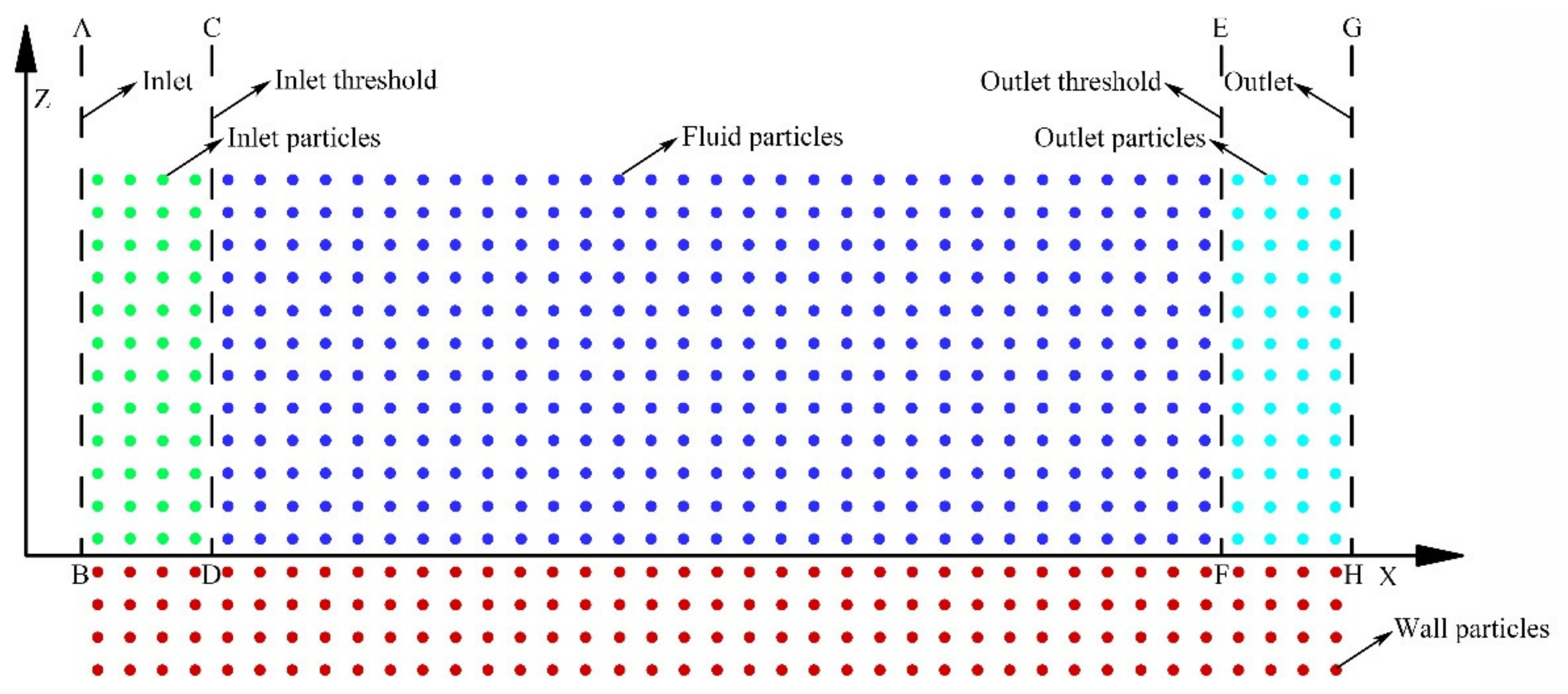
The layout of the computational domain is displayed in Figure 1. The boundary AB is the inlet boundary. The inlet threshold locates at boundary CD. The domain between AB and CD is the inlet boundary zone. The boundary EF is the outlet threshold. The outlet locates at boundary GH. The domain between EF and GH is the outlet boundary zone. The inlet/outlet boundaries are treated using inflow/outflow algorithms that were first developed by Federico et al. [9]. Initially, four-layer particles (Figure 1) are placed at the inlet (green particles) and outlet (light blue particles) boundary, respectively. Variables of the inlet particles are set to specific values. Following this, the inlet particles move forward based on the given velocity. Inlet particles transform into fluid particles when they enter the fluid domain. To maintain constant inlet particle numbers, new inlet particles are reproduced at upward of transformed inlet particles. As concerns the outlet boundary, it is possible to impose either free outflow conditions or specific outflow conditions (similar to inflow conditions). For free outflow conditions, fluid particles (blue particles) become outlet particles, and their variables are frozen when they flow across the outlet threshold EF. For specific outflow conditions, fluid particles become outlet particles and their variables are also frozen, with the exception of their velocity, which is artificially specified when they flow across the outlet threshold EF. Subsequently, the outlet particles move forward with the frozen velocity or specific velocity, until they flow out of the outlet boundary. For example, free outflow conditions were used in Section 3.2. Conversely, specific outflow conditions were used in Section 3.3 to form a subcritical outflow and obtain a hydraulic jump.
Solid wall boundaries are modeled using a fixed virtual particle technique [9,12]. Four-layer fixed wall particles (red particles) are constructed to represent the solid wall boundary (Figure 1). The positions of the wall particles remain unchanged during the simulation. However, the variables of wall particles, such as velocity, density, pressure, and so on, are obtained according to the mirror particles in the fluid domain by Moving Least Square interpolation. The mirroring of velocity for the slip and non-slip boundary is a little different. For the non-slip boundary, the tangential wall particles velocity is opposite to that of their mirror particles, while the magnitude is the same. However, the direction and magnitude of the tangential velocity are the same for the mirroring particles of the slip boundary. For the slip boundary, the tangential velocity magnitude and direction of the wall particles are equal to those of their mirroring particles. The normal wall particle velocity is of the same magnitude and opposite direction of mirroring particles for both boundary conditions.
2.3. Parallel Strategy
OpenMP is a parallel programming language for shared memory programming. The multithreading parallel of an existing programming language can be achieved by using the OpenMP to extend C language and Fortran languages. OpenMP can be accepted easily by programmers, with its unique portability, wide support of programming languages, and few APIs. The programming model of the OpenMP is based on the thread [13]. The functions of OpenMP are mainly implemented by compiling instructions. A compiler will recognize specific annotations, which contain certain semantics of the OpenMP, when the compiler compiles programs. In addition, the OpenMP can flexibly control the running of programs by changing the environment variables. For example, !$OMP PARALLEL is used to identify a parallel block in a Fortran program. A compiler will ignore these specific annotations as ordinary annotations if the compiler fails to recognize such semantics. Programmers can make full use of this property when they convert their serial program to a parallel program, so that the serial program can support parallel code without modifying the serial part of the code. With the above advantages, the OpenMP has attracted considerable attention from numerous researchers in recent years [13,14,15,16].
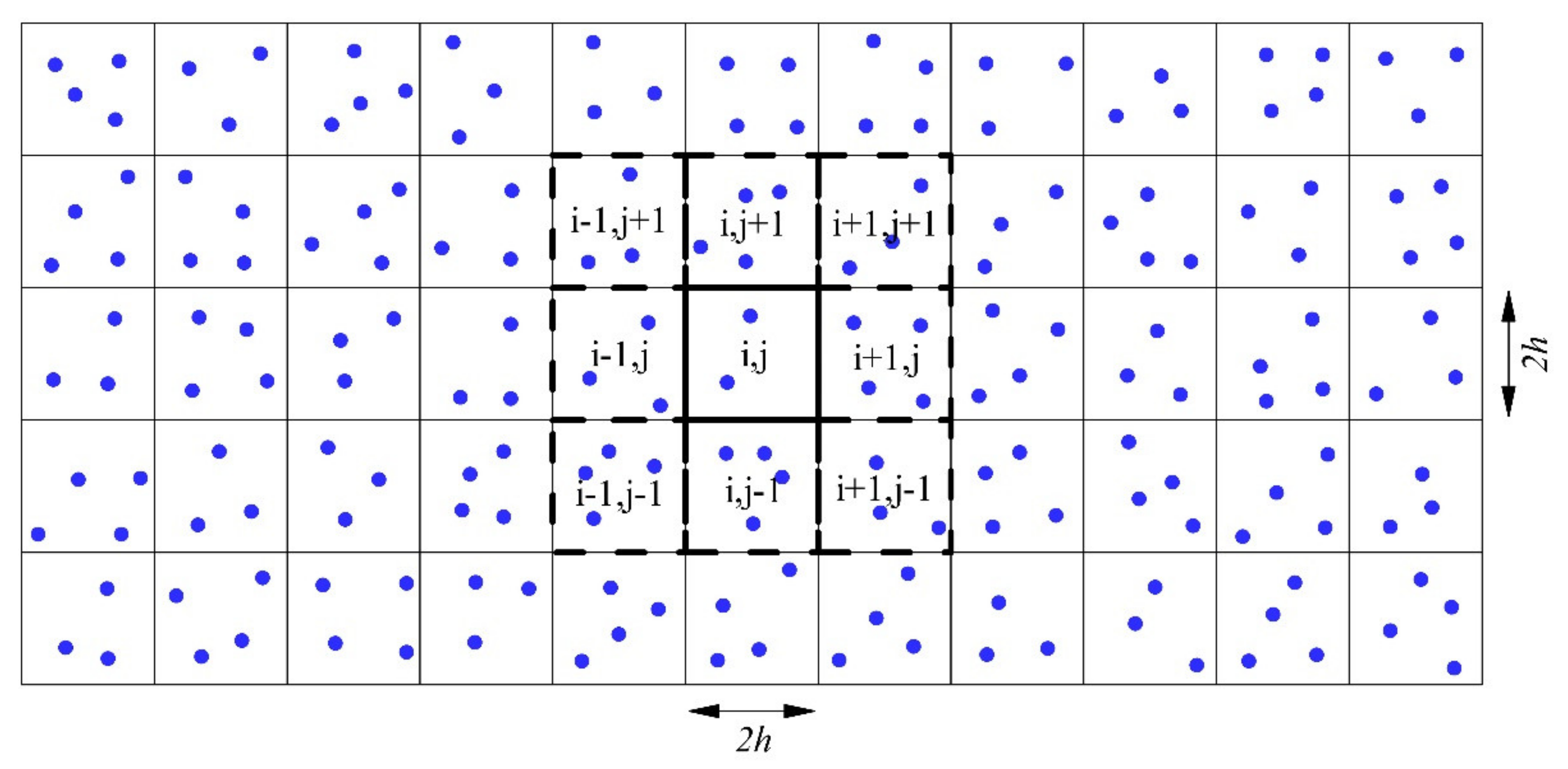
The SPH method explicitly solves ordinary differential equations, instead of solving traditional linear equations systems. The main time-consuming components are the loops of neighboring particle search and variable calculation. Therefore, the parallel strategy in this paper is to add OpenMP statements to time-consuming serial loops, causing these loops to be paralleled. In addition, a less time-consuming algorithm [13,17] is selected to search neighboring particles (Figure 2). This algorithm divides the computational domain into a series of square grids with a side length of 2h. Thus, it is possible for particles in each grid to interact only with those in an adjacent grid. Loss of time is greatly reduced compared with a direct search. Inlet and outlet particles are few, and generally do not number more than several hundred. Therefore, the loops for inlet and outlet particles are not paralleled, due to the less time-consuming procedure that may cause the loss of time of parallel code to be larger than that of the series code.
3. Numerical Test Cases
First, a performance analysis of the OpenMP parallel code was conducted to decide the parallel granularity. Then, two open channel flows were simulated to test the accuracy of the model. Finally, two test cases of hydraulic jumps with different Froude numbers were considered, to validate the accuracy of the model in computing the hydraulic jumps.
3.1. Performance Analysis on Environment Variables
Load balancing is one of the key factors affecting the performance of OpenMP multithreaded programs. According to the execution principle of OpenMP, waiting between threads in a parallel program, which will inevitably lead to the inefficiency of the parallel program, will be significantly longer if the load imbalance in OpenMP program cannot be effectively controlled. Static, dynamic, guided, and runtime are four main scheduling strategies in OpenMP [15]. Runtime scheduling was used to select one of the first three scheduling strategies based on the environment variable OMP_SCHEDULED in OpenMP. Therefore, runtime scheduling was not considered in the following calculations.
To the largest extent possible, all loop iterations were divided into blocks of the same size by Static scheduling. These iterations were divided equally if block size was not specified. n was assumed to be the total number of iterations. m was assumed to be the total number of threads in the parallel area. Subsequently, n/m iterations were assigned to every thread when the block size was the default. When the block size was set, successive iterations with the block size were assigned to each thread. Thus, the total workload was approximately divided into n/size blocks that were subsequently allocated to each thread in turn according to the rotation rule. An internal task queue was used by dynamic scheduling. A thread was allocated a certain number of iterations, specified by block size when it was available. When a thread completed its currently allocated block, the next block was taken from the head of the task queue. It should be noted that dynamic scheduling required additional overhead. Guided scheduling was similar to dynamic scheduling, to the extent that block size started large and subsequently decreased gradually. Therefore, guided scheduling was able to reduce the time to access queues for threads.
The parallel speed-up Rs is compared in Figure 3 for a hydraulic jump test case to test the efficiency of the parallel SPH code. In Figure 3, the coordinate x is the block size of the scheduling strategy. The coordinate y is the parallel speed-up Rs. The color of the line represents the scheduling strategy, where a red line is the result of a serial program. P1–P4 represent discrete particle numbers in the calculation domain. The parallel code runs on an Intel(R) Core (TM) i5 CPU with 2 cores, 4 threads, and a main frequency of 3.2 GHz. The total particle numbers are the sum of the boundary particles and the fluid particles at the initial time. These did not change much when the simulation became stable. The parallel speed-up was calculated as:
where tp represents the execution time of the parallel code while ts represents the execution time of the serial code.
In Figure 3, the parallel speed-up of serial code is 1.0, based on the parallel speed-up equation. The execution time is the average time of ten runs. Default scheduling achieves no acceleration, while it makes the parallel execution time greater than the serial execution time. The reason for this may be that all boundary particles are distributed to one core by default, due to the sequential iteration of fluid particles and boundary particles in the loop. Subsequently, the waiting time of the core dealing with boundary particles is long because the running time of the fluid particles is longer than that of the boundary particles. Ultimately, the parallel execution time is longer than the serial time due to an unbalanced load. The speed-up of the guided scheduling is not obvious and is relatively stable. The speed-up essentially did not change with block size, except as shown in Figure 3a. However, the speed-ups of static and dynamic scheduling re quite obvious. When particle numbers are less than 1 million, the parallel speed-up of static scheduling is higher than that of dynamic scheduling, while the opposite is true when particle numbers are greater than 1 million. All the maximum parallel speed-up of static scheduling was achieved at a block size of 10, except as shown in Figure 3c. For dynamic scheduling, the block size of the maximum parallel speed-up increased gradually from 20 to 100, as particle numbers increased. Therefore, static scheduling was selected and block size was set to 10, while a smaller particle number was considered for the 2D hydraulic jumps. These particle numbers are usually less than 0.2 million. At this point, the parallel speed-up could reach about 2.0.
3.2. Open Channel Flow
Two uniform laminar flow test cases of open channels [18] were simulated. The length of the numerical channel was 1.0 m. The slope was 0.04% for case 1 and 0.1% for case 2. The corresponding initial water depth h0 was 0.1 m and 0.2 m, respectively. To obtain laminar flow, the dynamic viscosity μ was set to 1.0 10−1 Ns/m2 for case 1 and 6.0 10−1 Ns/m2 for case 2, respectively. The Reynolds numbers of the two test cases were 200 and 100. The channel bed was the non-slip boundary. A uniform velocity that was calculated using the formula in [9] was given to the inlet particles. The outlet boundary was free outflow. To analyze the adequacy of the particles, Figure 4 compares the velocity profile between the numerical results with different particle spacing and analytical solutions. The numerical results with a particle spacing h/Δx = 20 show a good agreement with the analytical solutions. Therefore, the particle spacing should ensure that the particle numbers along the water depth are not less than 20.
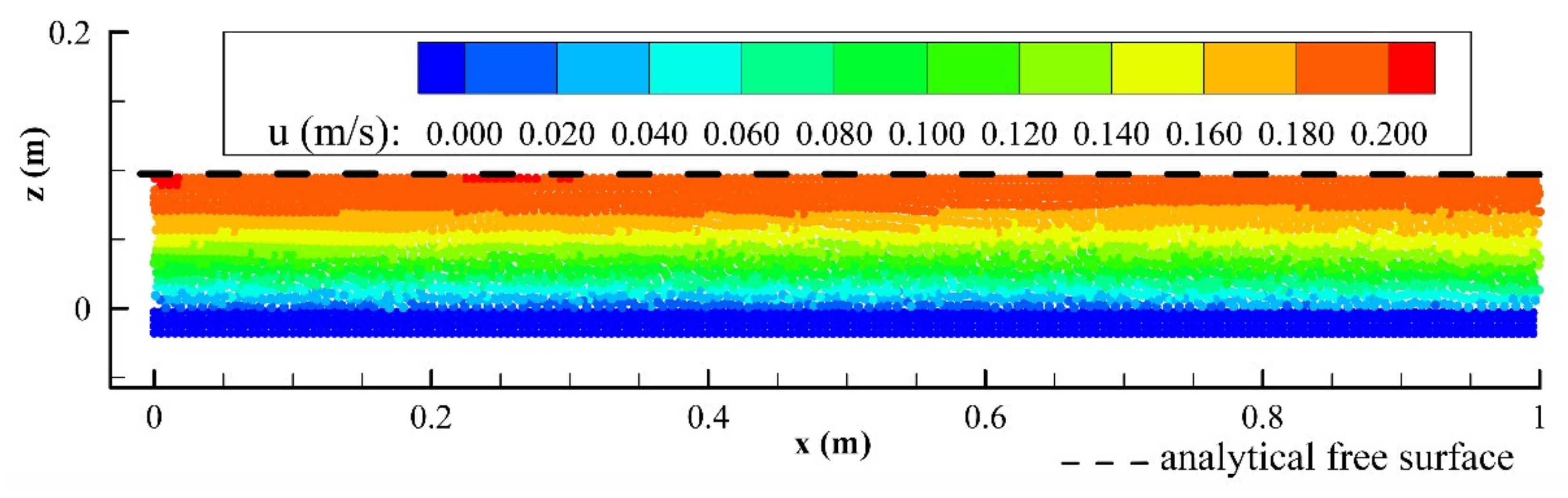
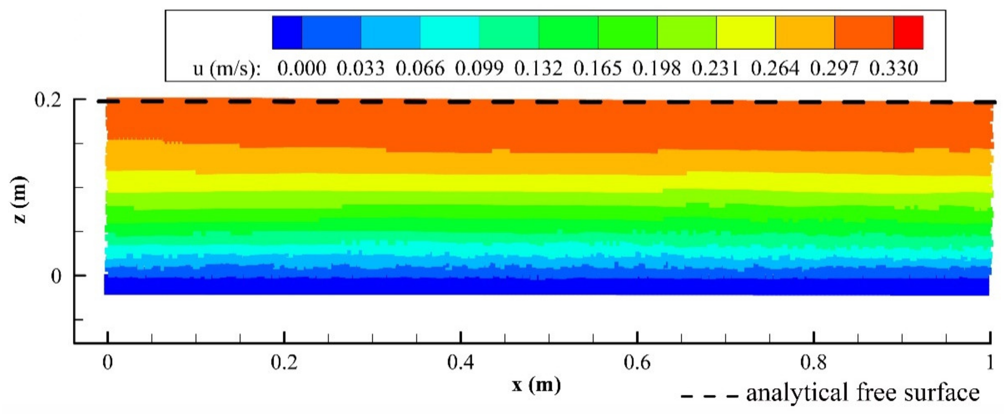
Figure 5 and Figure 6 show the stable velocity fields of case 1 and case 2, respectively. The channel length of 1.0 m does not include the development area of the outlet and inlet flow. The wall boundary particles are shown in these figures. The numerical results show a uniform distribution for the velocity. Meanwhile, the calculated water level in channels is consistent with the analytical free surface. Similar results of flow pattern were achieved by Federico et al. [9] and Tan et al. [18]. In addition, quite smooth pressure fields were also obtained. The results suggest that the influence of a Shepard filter on open channel flow is not obvious.
To analyze the numerical results quantitatively, comparisons of the velocity profiles between numerical results and analytical solutions of case 1 and 2 were made, as depicted in Figure 4. The numerical velocity profiles with h/Δx = 20 show good consistency with the analytical data. The numerical results of the velocity in Figure 4 are average values of a series of the cross-section in the calculation domain. The L2 errors between the analytical and numerical velocity are given in Table 1. The L2 errors with h/Δx = 20, which is less than or equal to 0.05, are quite small. This suggests that the present SPH model can accurately simulate the uniform laminar flow
where N is the simple numbers; and are the numerical result and the analytical solution at position i, respectively.
3.3. Hydraulic Jumps
To validate the model, two test cases of hydraulic jumps [9] were selected to compare the numerical conjugate water depths with the analytical data that were calculated by the conjugate depth formula for ideal fluid. The inflow Froude numbers were = 1.15 for case 1 and 1.88 for case 2. The corresponding types of hydraulic jumps were set to undular jump and full jump. For all the test cases, the inlet water depth h1 was always 0.01 m. The outlet conjugate water depths obtained from the analytical formula were 0.012 m and 0.022 m for case 1 and case 2, respectively. The length of the numerical horizontal flume was L = 40h1. The inlet boundary conditions were specific uniform velocity U1 and water depth h1. The outlet boundary conditions were specific uniform velocity U2. For the solid wall boundary, the slip boundary condition was adopted. The initial water level and velocity in the computational domain were specific uniform velocity U2 and water depth h1. The initial pressure and density were calculated based on the hydrostatic pressure hypothesis. For ideal fluid, the viscosity was ignored. Therefore, the model was extended to simulate the inviscid flow by replacing the dynamic viscosity with an artificial viscosity coefficient. This artificial viscosity was mainly adopted to keep stability of calculation. Here, a formula was used. Following the study of Federico et al. [9], α = 0.02 was taken. It was found that the pressure fields were noisy when the Fr1 was large. This noisiness of pressure fields was not found in Federico et al. [9], because only velocity fields of hydraulic jumps were provided, while pressure fields were not considered. Therefore, a Shepard filter was introduced into the model. To reduce loss of time, the Shepard filter was calculated every 30-time step, which proved to be sufficient [19]. The equation is where . The space between particles was 0.005 m. Total time of 16 s was simulated.
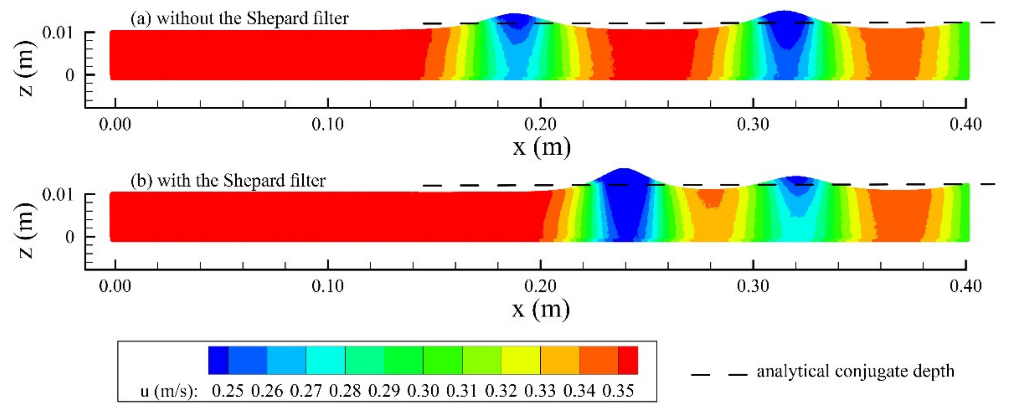
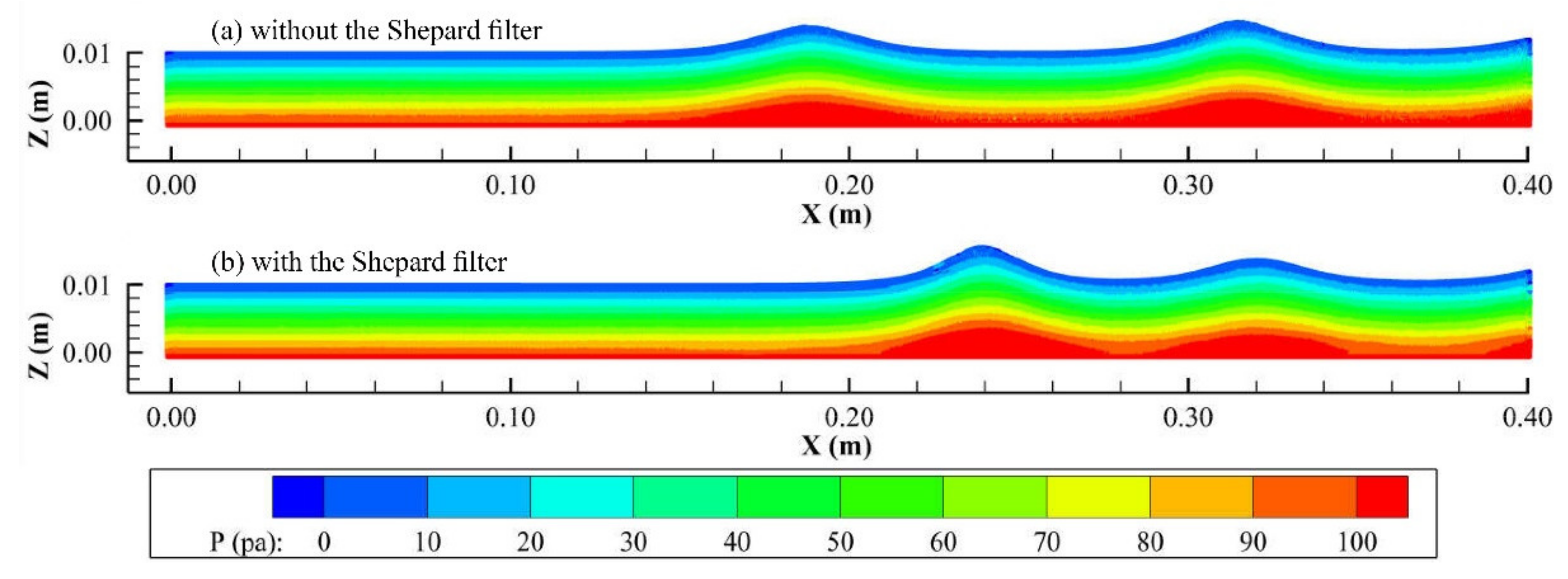
Figure 7 shows the velocity fields of case 1 at t = 15.96 s. This time instant was approximately identical to the time used in [9]. Figure 8 shows the pressure fields of case 1 at the same instantaneous time. The velocity fields without the Shepard filter yielded results that were similar to those of Federico et al. [9]. Both water depths at the outlet boundary with and without the filter displayed good consistency with the analytical conjugate depth. All the four wave crests showed an overprediction with the errors of 0.002 m, 0.0025 m, 0.0035 m, and 0.0015 m, respectively. For the calculated results without the Shepard filter, the first wave crest was slightly lower than the second one. This phenomenon does not coincide with the general characteristics of undular hydraulic jumps, which display free surface undulations of decreasing amplitude [8,20]. The results with the Shepard filter displayed a free surface undulation with decreasing amplitude. Comparing the results of Figure 7b with those of Figure 7a, the first crest with the filter is higher than the one without the filter, while the second crest is the opposite. In addition, the results with the Shepard filter display a shorter distance between the two crests than those without the Shepard filter. The pressure fields of case 1 at t = 15.96 s are shown in Figure 8. Both the field results with and without the Shepard filter show a uniform distribution of pressure. Thus, the Shepard filter does not obviously improve the pressure fields for a low Fr1.
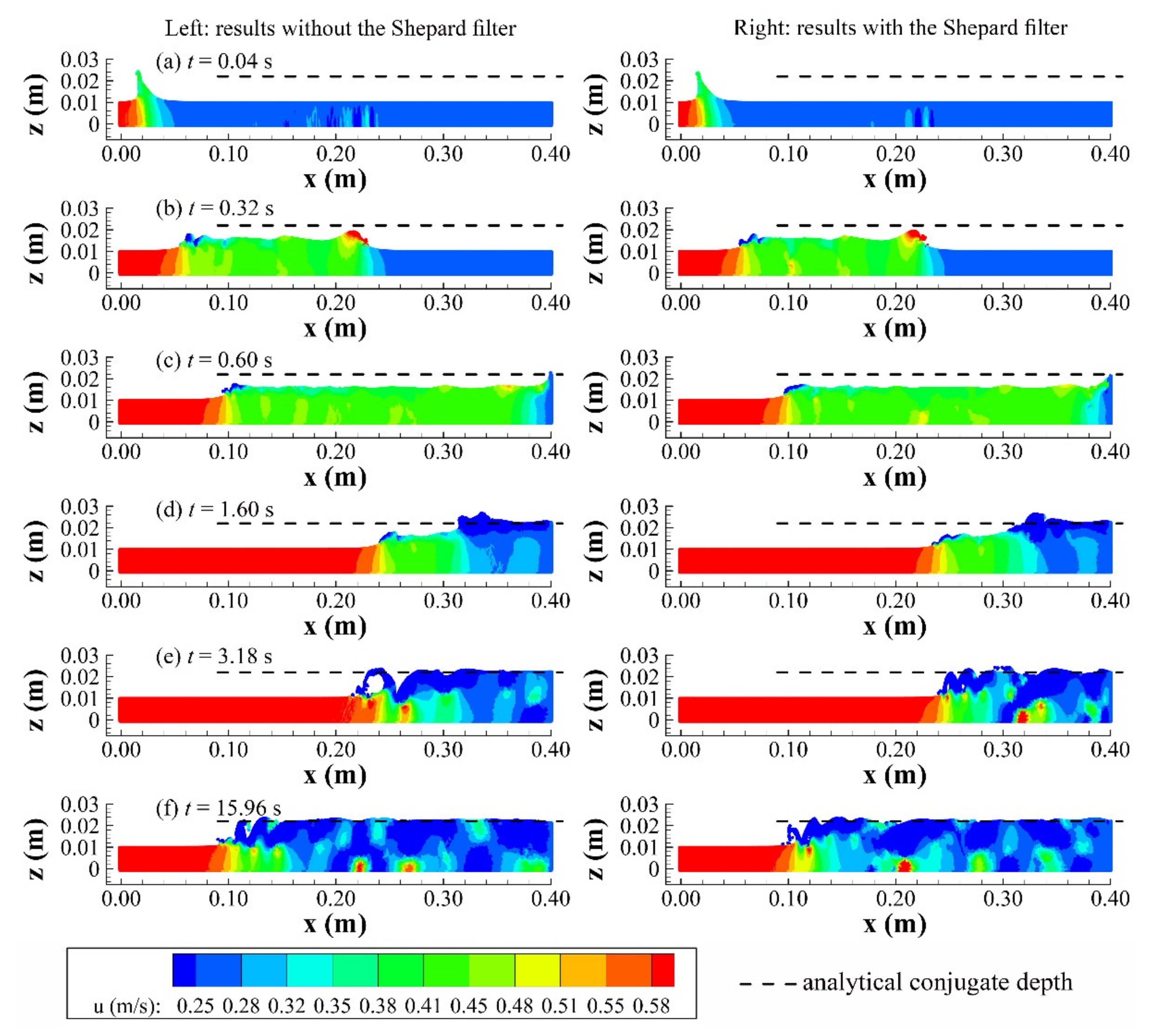
The velocity fields of case 2 at certain instantaneous times are shown in Figure 9. The flow patterns of the two sets of results with and without the filter are similar. The inflow with larger speed interacts with the initial slow flow and hydraulic jumps at t = 0.04 s. At t = 0.32 s, two shock waves are formed and propagate downstream with distinct velocities. Until t = 0.6 s, when the faster shock wave arrives at the outlet boundary and reflects upstream. The reflected wave merges with the slower shock wave and propagates continuously upstream at t = 1.6 s and 3.18 s. The flow fields essentially achieve dynamic stabilization when the jump toe oscillates around t = 0.1 m. In addition, the results with the filter show slightly smoother velocity fields in Figure 9. The calculated conjugate depth with the filter is more consistent with the analytical conjugate depth than that without the filter when the flow reaches a quasi-static state.
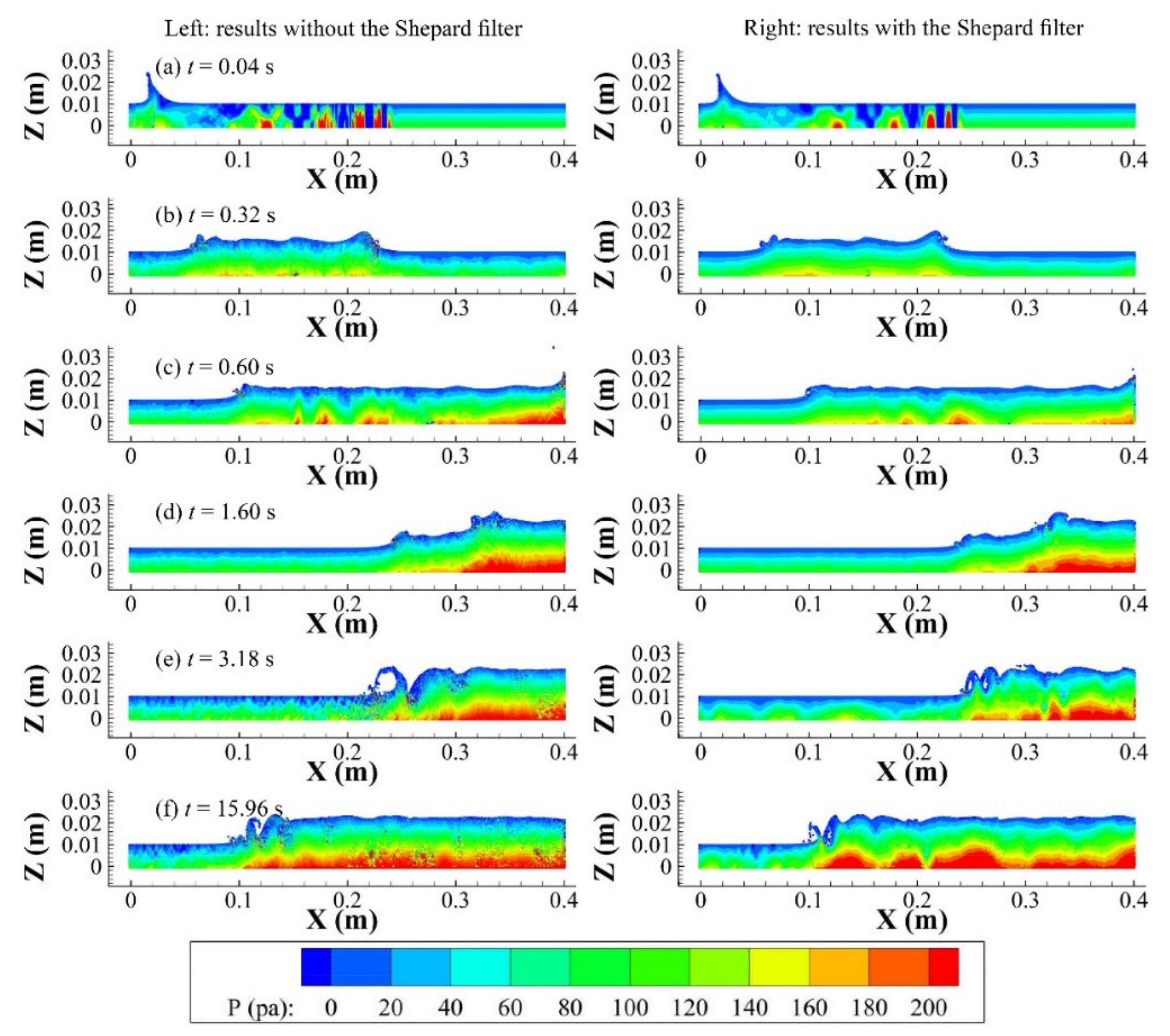
In Figure 10, pressure fields of case 2 are given. The pressure fields without the Shepard filter are noisy while the pressure fields with the Shepard filter exhibit much more uniform and smoother results during the entire simulation. Meanwhile, the pressure fields evolve into relatively uniform fields after a short time of about 0.32 s.
4. Conclusions
A parallel WCSPH model with Shepard density filter was established to efficiently and accurately reproduce 2D hydraulic jumps. The WCSPH model was accelerated by the OpenMP. To further reduce execution time, the performance of the OpenMP-based SPH code with different scheduling strategy was compared for the test case of hydraulic jumps. The comparison of the parallel speed-ups under different particle numbers shows that static scheduling in OpenMP has a higher acceleration on the serial code for the 2D hydraulic jumps. By calculating and analyzing the acceleration of static scheduling with different block sizes, static scheduling with a block size of 10 was adopted for the parallel code. To validate the accuracy of the model, two test cases of open channel uniform flows and hydraulic jumps were simulated. The calculated results of the fluid velocity and surface elevation showed very good consistency with the analytical data. Meanwhile, the numerical conjugate depths of the hydraulic jumps were consistent with the analytical data, which suggests that the model works well in calculating hydraulic jumps. The numerical conjugate depth with the Shepard filter is more nearly identical to the analytical conjugate depth than that without the filter when the flow reached quasi-static state. Furthermore, the velocity and pressure fields of the hydraulic jumps test cases show that the WCSPH model with Shepard density filter can smooth the pressure fields without an obvious effect on the velocity fields when the inflow Froude number is relatively large. In short, the present parallel SPH model can efficiently and accurately simulate open channel flow and hydraulic jumps.
Author Contributions
Formal analysis, J.L.; Investigation, J.L. and H.M.; Methodology, J.L. and B.J.; Software, S.J.; Supervision, X.P.; Validation, W.D.; Writing—original draft, J.L.; Writing—review and editing, H.M. and W.D. All authors have read and agreed to the published version of the manuscript.
Funding
This work was supported by the National Natural Science Foundation of China (Grant No. 52001071 and 52071090); the Youth Innovative Talent Project of the Guangdong Education Bureau (Grant No. 2019KQNCX045); the Doctor Initiate Projects of Guangdong Ocean University (Grant No. 060302072103); and “First Class” Provincial Financial Special Fund Construction Project of Guangdong (Grant No. 231419010).
Conflicts of Interest
The authors declare no conflict of interest.
References
- Azimi, H.; Shabanlou, S.; Kardar, S. Characteristics of Hydraulic Jump in U-Shaped Channels. Arab. J. Sci. Eng. 2017, 42, 3751–3760. [Google Scholar] [CrossRef]
- Babaali, H.; Shamsai, A.; Vosoughifar, H. Computational Modeling of the Hydraulic Jump in the Stilling Basin with Convergence Walls Using CFD Codes. Arab. J. Sci. Eng. 2015, 40, 381–395. [Google Scholar] [CrossRef] [Green Version]
- Gharangik, A.M.; Chaudhry, M.H. Numerical Simulation of Hydraulic Jump. J. Hydraul. Eng. 1991, 117, 1195–1211. [Google Scholar] [CrossRef]
- Unami, K.; Kawachi, T.; Munir Babar, M.; Itagaki, H. Estimation of diffusion and convection coefficients in an aerated hydraulic jump. Adv. Water Resour. 2000, 23, 475–481. [Google Scholar] [CrossRef]
- López, D.; Marivela, R.; Garrote, L. Smoothed particle hydrodynamics model applied to hydraulic structures: A hydraulic jump test case. J. Hydraul. Res. 2010, 48, 142–158. [Google Scholar] [CrossRef]
- Jonsson, P.; Jonsén, P.; Andreasson, P.; Lundström, T.S.; Hellström, J.G.I. Smoothed Particle Hydrodynamic Modelling of Hydraulic Jumps: Bulk Parameters and Free Surface Fluctuations. Engineering 2016, 8, 386–402. [Google Scholar] [CrossRef] [Green Version]
- Gu, S.; Ren, L.; Wang, X.; Xie, H.; Huang, Y.; Wei, J.; Shao, S. SPhysics simulation of experimental spillway hydraulics. Water 2017, 9, 973. [Google Scholar] [CrossRef] [Green Version]
- De Padova, D.; Mossa, M.; Sibilla, S.; Torti, E. 3D SPH modelling of hydraulic jump in a very large channel. J. Hydraul. Res. 2013, 51, 158–173. [Google Scholar] [CrossRef]
- Federico, I.; Marrone, S.; Colagrossi, A.; Aristodemo, F.; Antuono, M. Simulating 2D open-channel flows through an SPH model. Eur. J. Mech. 2012, 34, 35–46. [Google Scholar] [CrossRef]
- Molteni, D.; Colagrossi, A. A simple procedure to improve the pressure evaluation in hydrodynamic context using the SPH. Comput. Phys. Commun. 2009, 180, 861–872. [Google Scholar] [CrossRef]
- Altomare, C.; Crespo, A.J.C.; Domínguez, J.M.; Gómez-Gesteira, M.; Suzuki, T.; Verwaest, T. Applicability of Smoothed Particle Hydrodynamics for estimation of sea wave impact on coastal structures. Coast. Eng. 2015, 96, 1–12. [Google Scholar] [CrossRef]
- Marrone, S.; Antuono, M.A.G.D.; Colagrossi, A.; Colicchio, G.; Le Touzé, D.; Graziani, G. δ-SPH model for simulating violent impact flows. Comput. Methods Appl. Mech. Eng. 2011, 200, 1526–1542. [Google Scholar] [CrossRef]
- Yeylaghi, S.; Moa, B.; Oshkai, P.; Buckham, B.; Crawford, C. ISPH modelling of an oscillating wave surge converter using an OpenMP-based parallel approach. J. Ocean Eng. Mar. Energy 2016, 2, 301–312. [Google Scholar] [CrossRef] [Green Version]
- Ihmsen, M.; Akinci, N.; Becker, M.; Teschner, M. A parallel SPH implementation on multi-core CPUs. Comput. Graph. Forum 2011, 30, 99–112. [Google Scholar] [CrossRef]
- Zhang, S.; Xia, Z.; Yuan, R.; Jiang, X. Parallel computation of a dam-break flow model using OpenMP on a multi-core computer. J. Hydrol. 2014, 512, 126–133. [Google Scholar] [CrossRef]
- Crespo, A.J.C.; Domínguez, J.M.; Rogers, B.D.; Gómez-Gesteira, M.; Longshaw, S.; Canelas, R.; Vacondiod, R.; Barreiro, A.; García-Feal, O. DualSPHysics: Open-source parallel CFD solver based on Smoothed Particle Hydrodynamics (SPH). Comput. Phys. Commun. 2015, 187, 204–216. [Google Scholar] [CrossRef]
- Gomez-Gesteira, M.; Rogers, B.D.; Crespo, A.J.C.; Dalrymple, R.A.; Narayanaswamy, M.; Dominguez, J.M. SPHysics—Development of a free-surface fluid solver—Part 1: Theory and formulations. Comput. Geosci. 2012, 48, 289–299. [Google Scholar] [CrossRef]
- Tan, S.K.; Cheng, N.S.; Xie, Y.; Shao, S. Incompressible SPH simulation of open channel flow over smooth bed. J. Hydro-Environ. Res. 2015, 9, 340–353. [Google Scholar] [CrossRef] [Green Version]
- Gomez-Gesteira, M.; Crespo, A.J.C.; Rogers, B.D.; Dalrymple, R.A.; Dominguez, J.M.; Barreiro, A. SPHysics—Development of a free-surface fluid solver—Part 2: Efficiency and test cases. Comput. Geosci. 2012, 48, 300–307. [Google Scholar] [CrossRef]
- Chanson, H.; Montes, J.S. Characteristics of Undular Hydraulic Jumps: Experimental Apparatus and Flow Patterns. J. Hydraul. Eng. 1995, 121, 129–144. [Google Scholar] [CrossRef] [Green Version]
Figure 1.
Sketch of the computational domain.

Figure 2.
Sketch of the neighboring particles searching.

Figure 3.
Parallel speedup of the OpenMP.

Figure 4.
Comparisons of the velocity profiles between numerical results and analytical solutions.

Figure 5.
Velocity fields of case 1.

Figure 6.
Velocity fields of case 2.

Figure 7.
Velocity fields of case 1 at t = 15.96 s.

Figure 8.
Pressure fields of case 1 at t = 15.96 s.

Figure 9.
Velocity fields of case 2.

Figure 10.
Pressure fields of case 2.


Table 1.
L2 errors between the numerical and analytical velocity.
| Test Cases | Case 1 | Case 2 |
|---|---|---|
| h/Δx = 10 | 0.05 | 0.06 |
| h/Δx = 20 | 0.03 | 0.05 |
Publisher’s Note: MDPI stays neutral with regard to jurisdictional claims in published maps and institutional affiliations. |
© 2021 by the authors. Licensee MDPI, Basel, Switzerland. This article is an open access article distributed under the terms and conditions of the Creative Commons Attribution (CC BY) license (https://creativecommons.org/licenses/by/4.0/).
Share and Cite
MDPI and ACS Style
Lin, J.; Mao, H.; Ding, W.; Jia, B.; Pan, X.; Jin, S. Numerical Simulations of 2D Hydraulic Jumps by a Parallel SPH Model. Water 2021, 13, 2536. https://doi.org/10.3390/w13182536
AMA Style
Lin J, Mao H, Ding W, Jia B, Pan X, Jin S. Numerical Simulations of 2D Hydraulic Jumps by a Parallel SPH Model. Water. 2021; 13(18):2536. https://doi.org/10.3390/w13182536
Chicago/Turabian StyleLin, Jinbo, Hongfei Mao, Weiye Ding, Baozhu Jia, Xinxiang Pan, and Sheng Jin. 2021. "Numerical Simulations of 2D Hydraulic Jumps by a Parallel SPH Model" Water 13, no. 18: 2536. https://doi.org/10.3390/w13182536
Note that from the first issue of 2016, this journal uses article numbers instead of page numbers. See further details here.