Assessment of Ensemble Models for Groundwater Potential Modeling and Prediction in a Karst Watershed

Abstract

Due to numerous droughts in recent years, the amount of surface water in arid and semi-arid regions has decreased significantly, so reliance on groundwater to meet local and regional demands has increased. The Kabgian watershed is a karst watershed in southwestern Iran that provides a significant proportion of drinking and agriculture water supplies in the area. This study identified areas with karst groundwater potential using a combination of machine learning and statistical models, including entropy-SVM-LN, entropy-SVM-SG, and entropy-SVM-RBF. To do this, 384 karst springs were identified and mapped. Sixteen factors that are related to karst potential were identified from a review of the literature, and these were compiled for the study area. The 384 locations were randomly separated into two categories for training (269 location) and validation (115 location) datasets to be used in the modeling process. The ROC curve was used to evaluate the modeling results. The models used, in general, were good at determining the location of karst groundwater potential. The evaluation showed that the E-SVM-RBF model had an area under the curve of 0.92, indicating that it was most accurate estimator of groundwater potential among the ensemble models. Evaluation of the relative importance of each of the 16 factors revealed that land use, a vector ruggedness measure, curvature, and topography roughness index were the most important explainers of the presence of karst groundwater in the study area. It was also found that the factors affecting the presence of karst springs are significantly different from non-karst springs.

1. Introduction

In recent decades, reduced availability of water in alluvial sediments and the increasing demand for water has led to increased exploitation of groundwater in hard rock and calcareous geological formations. Due to their low salt content, hard rock formations yield water of good quality [1]. Such aquifers could help to provide water for drinking, agriculture, and industrial uses [2]. Limestone and dolomite formations can develop karst landscapes that contain fractures, voids, and conduits that can serve as aquifers. It is estimated that karst covers approximately 7–12% of the Earth’s continental surface [3]. Fifteen to 25% of the world’s population depends on karst formations for fresh water [4].

Surface water is scarce in karst regions, but groundwater is more common than in other areas. Fractures and cracks create hydraulic pathways through the rock [5]. The hydrogeological structure of aquifers in karst areas is unique [6]. The most prominent feature of these aquifers is the great variation in hydrodynamic properties. The study of aquifers to determine groundwater potential in karst regions can be very expensive due to the difficulty of using exploratory drilling and well monitoring to assess groundwater in heterogeneous formations [7,8]. The presence of springs are especially important indicators of groundwater in karst regions. According to Chrysik and Stanovich [9], springs can be indicators of the internal characteristics of an aquifer. The identification of groundwater in regions with artesian springs can be made easier and less expensive by using low-cost methods such as statistical and machine learning models.

Karst aquifer recharge depends on various natural factors such as climate, topography, vegetation, soil, and geology [2,10,11]. Choosing a suitable method for assessing water infiltration is often controversial. Geographic information systems (GISs) are powerful tools for classifying, analyzing, and retrieving information, and have been used to replace exploration and spatial experimentation in the field [12,13,14]. Saving time and money, the ability to perform complex spatial and non-spatial data analyses, and flexibility are features of GISs and these have made them attractive for groundwater study [15,16].

Various methods and models have been used to determine groundwater potential in specific landscapes. Multi-criteria decision-making methods (MCDMs), statistical methods, and hydrogeological and machine learning models are some of these approaches. Applications of data mining, machine learning, and statistical methods have been advancing in groundwater research. The most important algorithms that have been used include logistic regression (LR), artificial neural network (ANN) [17], random forest (RF) [18], frequency ratio (FR) [19], evidential belief function (EBF) [20], random subspace (RS) [21,22], neuro-fuzzy inference system (ANFIS) [23], and classification and regression tree (CRT) [18].

The following are some of the studies conducted in the field of groundwater potential mapping using machine learning and statistical models: Zabihi et al. (2015) mapped groundwater potential using the Shannon entropy and random forest models in the Bojnourd plain of North Khorasan. The results of receiver operating characteristic (ROC) assessments indicated that very good accuracy was achieved with the Shannon entropy model (85.55%), but the random forest results were great (95.76%). Comparing random forest to the Shannon entropy model revealed that certain classes of the distance to a river, lithology, land use, and elevation factors had the greatest impacts on the groundwater potential. Chen et al. (2018) examined the ensemble of evidence weighting with functional tree data-mining methods. Their results showed excellent performances by the data mining ensemble methods for predicting groundwater potential. They developed three new hybrid artificial intelligence (AI) models that combined modified RealAdaBoost (MRAB), bagging (BA), and rotating forest (RF) with functional tree (FT) to map groundwater potential in a basalt landscape in DakLak Province, Highland Centre, Vietnam. They used the locations of 130 groundwater wells and 12 topographic and geo-environmental factors to predict groundwater. The models’ performances were evaluated using area under the curve (AUC) and other metrics. The results showed that although all of the hybrid models increased the fit and accuracy of prediction, the MRAB-FT (AUC = 0.742) model performed better than RF-FT (AUC = 0.736), BA-FT (AUC = 0.714), and single FT (AUC = 0.674). The MRAB-FT model is a promising hybrid AI technique for groundwater prediction. Rahmati et al. (2020) used new approaches based on Gini-, entropy- and ratio-based classification trees to predict the spatial patterns of groundwater potential in the mountains of Iran. They used 362 springs and several geo-environmental and topo-hydrological factors (slope, aspect, elevation, topographic wetness index (TWI), distance from the fault, distance from the river, rainfall, land use, lithology, plan curvature, and topographic roughness index (TRI)) to predict groundwater. Their results showed that Gini (AUC = 0.865) produced the best results, followed by the entropy (AUC = 0.847) and ratio (AUC = 0.859) models. Lithology provided the greatest impact on groundwater presence. Another study used individual and ensemble machine learning models to predict groundwater potential. Random forest (RF), logistic regression (LR), decision tree (DT), and artificial neural networks (ANNs) were the tested. The locations of approximately 374 groundwater springs were determined and 24 factors were selected based on information gain. The 15 model combinations were ranked using the compound factor (CF) method. Based on the success rates, the ensemble models were the most effective for mapping groundwater potential in mountain aquifers. The most efficient model, based on AUC evaluation, was the RF-LR-DT-ANN ensemble. Prioritization ranking indicated that the best models were the RF-DT and RF-LR-DT ensembles. Machine learning and statistical models have been shown to produce accurate groundwater potential maps, so review and evaluation of other models may improve the accuracy of predictive mapping. They could also save time and money in the search for groundwater in karst regions.

Aquifers are important water resources in the study area, so identifying areas with hidden groundwater is critical. Groundwater has been studied extensively, but few studies have been conducted in regions of karst formations. This study aimed to identify groundwater in karst areas using new statistical and machine learning methods. Analysis of karst groundwater potential in the Kabgian watershed was performed using a new statistical and machine learning ensemble. The innovation of this research is that it combines the entropy statistical model with different kernels of the SVM model. This led to the creation of several hybrid models: Entropy-SVM-RBF, entropy-SVM-LN, and entropy-SVM-SIG. These ensembles have not been previously used to map groundwater potential in a karst setting.

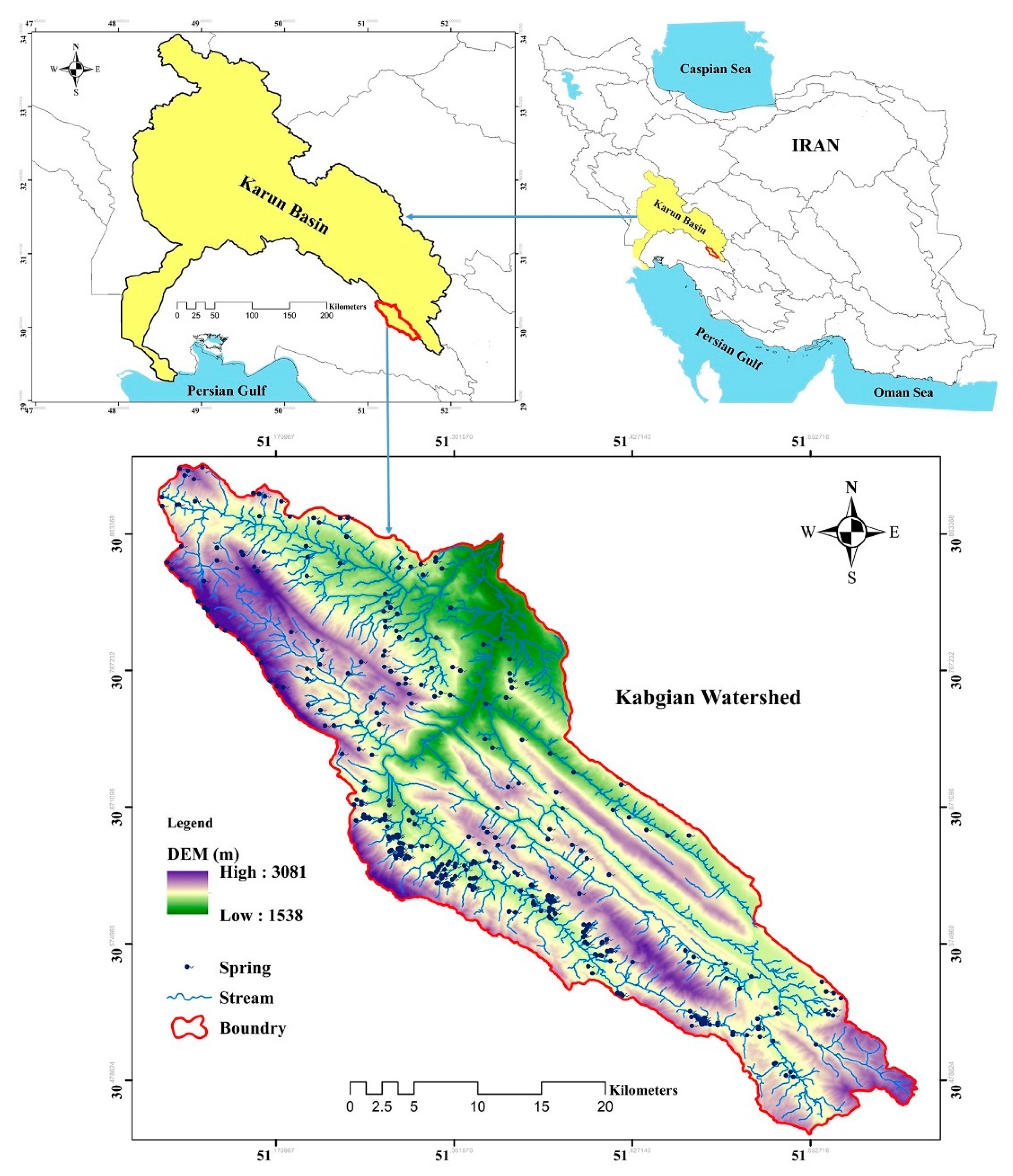
Description of the Study Area

The Kabgian watershed (defined by limits at 30°27′45.2″–30°54′40.1″ N, and 51°06′31.7″–51°37′14.1″ E). The watershed covers 873 km² and is located in the Karun basin in southwest Iran (Figure 1). The elevations range from 1538 to 3081 m. The mean annual precipitation is 787 mm and the mean annual air temperature is 13.5 °C (based on data from 1995 to 2019). More than 90% of annual rainfall occurs from November to May. Trees (particularly Quercus brantii), shrubs (Astragalus sp.), grass (Poaceae), and rocky outcrops cover the watershed. According to the 1:100,000 geological map prepared by the Geological Survey of Iran, the watershed’s geology was formed from the Mesozoic era to the present day. The lithology, oldest to newest, includes Neyriz, Sarvak, Gurpi, Pabdeh, Asmari, Gachsaran, Razak, Bakhtiari, and Quaternary formations (

Table 1. Lithological characteristics of the Kabgian watershed.

Age			Symbol	Lithology	Formation	Area		Karstification Potential
Era	Period	Epoch				ha	%
Cenozoic	Quaternary	-	Q	Alluvial sediments	Quaternary	10,282	11.77	No
	Tertiary	Pliocene	Bk	Conglomerate	Bakhtiari	1605	1.84	No
		Miocene	Ra	Marl and conglomerate	Razak	223	0.26	No
		Miocene	Gs	Gypsum/anhydrite, limestone, and marl	Gachsaran	15,164	17.36	Yes
		Oligomiocene	As	Limestone and dolomite	Asmari	43,339	49.63	Yes
		Paleocene	Pd	Marl	Pabdeh	9414	10.78	No
Mesozoic	Cretaceous	Campanian	Gu	Marl	Gurpi	1841	2.11	No
		Albian-Turonian	Sr	Limestone	Sarvak	5371	6.15	Yes
	Jurassic	Lias	Ne	Limestone and dolomite	Neyriz	87	0.1	Yes
Total						87,326	100	73.36%

). A large portion of the watershed is underlain by soluble formations of limestone, dolomite, and gypsum, thus the potential for karstification is high. More than 73% of the formations are karstic. Due to rainfall amounts, low average temperature, and the extent of karst, one can expect there to be significant groundwater in the watershed. Aquifers are, in fact, discharged by at least 384 springs.

2. Materials and Methods

2.1. Karst Groundwater Potential (KGP) Inventory Map

Karst aquifers do not have a typical volume. Their extent, geometry, and functioning can only be known through a study of karstification in their proximity. Unlike aquifers in porous matrices, the study and modeling of karst aquifers are complex [24]. Using modeling to determine groundwater potential has improved the ease of identification and exploitation of these features; this has been carried out most often in non-karst regions [25]. Karst groundwater potential mapping provides a way to integrate multiple data sources to delineate the areas that have greater groundwater potential [7]. Springs are the visible points of a karst system. The quantity and quality of their discharge water depends on the condition of the karst system. The presence of springs, therefore, is one of the most important indicators of an aquifer. Hence, a correlation between springs (the dependent variable) and environmental indicators (independent variables) hints at the potential spatial distribution of groundwater [26]. In this study, 384 active and inactive karst spring locations were obtained from Yasouj’s water resources department. Additionally, 384 non-springs were randomly generated in ArcGIS software. In order to model these points, they were divided into the two categories of validation (30%) and training (70%).

2.2. Factors Influencing Groundwater in Karst Regions (FIGKRs)

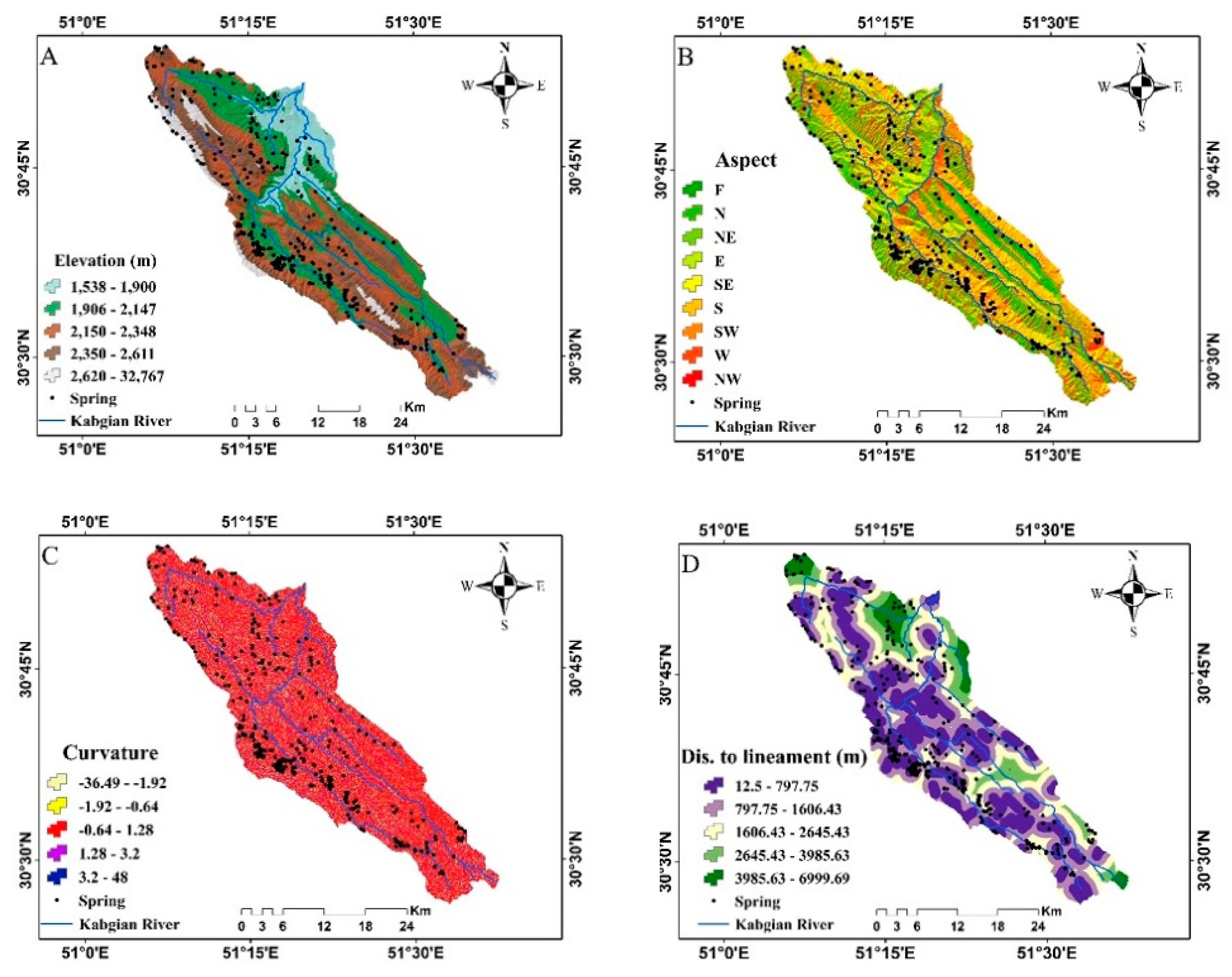
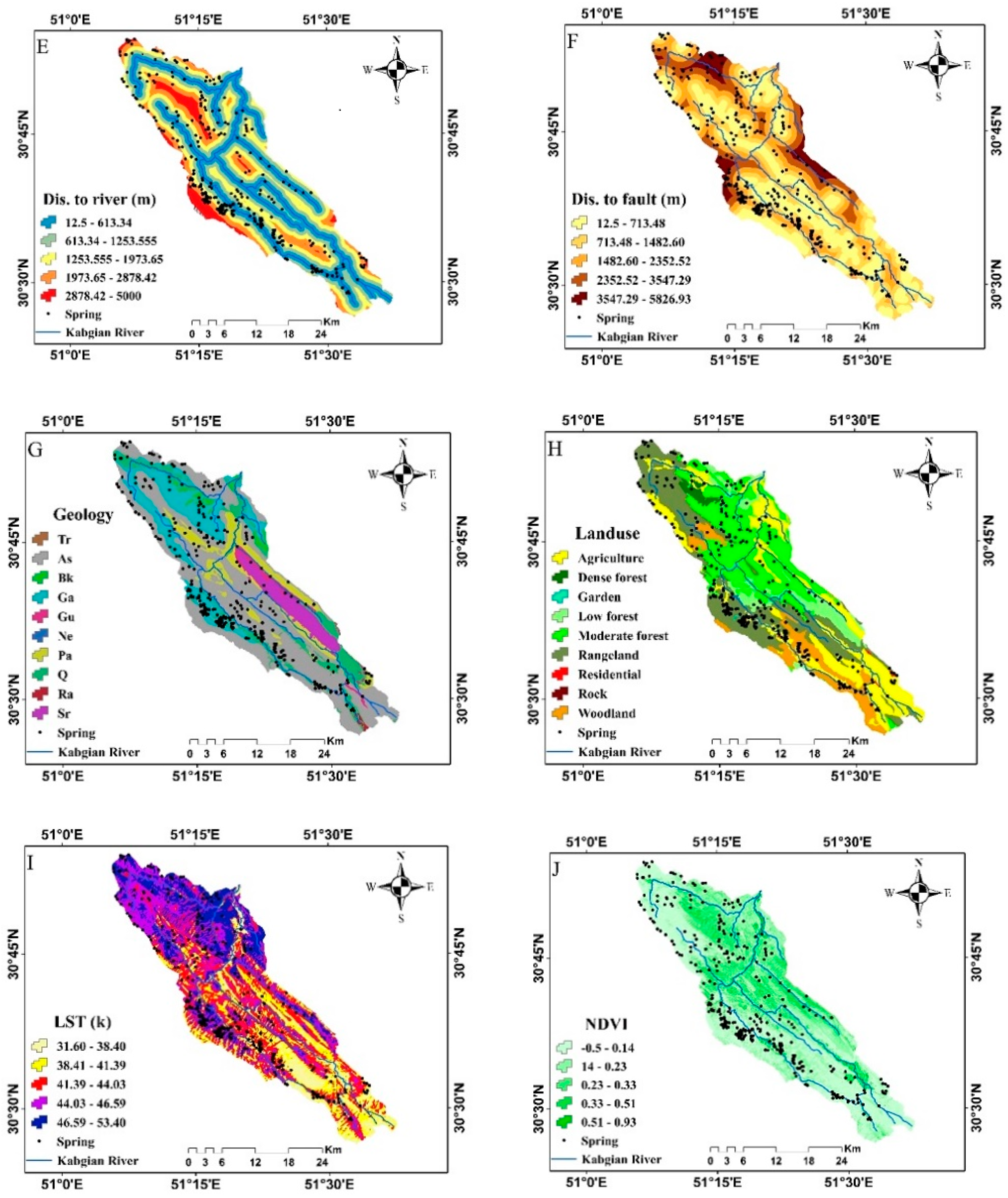
A number of characteristics can be associated with groundwater potential in a karst region. Based on a literature review and the conditions of the study area, 17 conditions—slope, aspect, elevation, topographic wetness index (TWI), land use, distance from the stream, distance from the fault, distance from the lineament, lithology, curvature, NDVI, rainfall, topography position index (TPI), topography roughness index (TRI), vector ruggedness measure (VRM), and land surface temperature (LST)—were identified as potential inputs into a predictive model [27,28,29]. These layers were prepared using ArcGIS 10.5, ENVI 5.3, Saga 3.2, Google Earth Pro software. Moreover, the base map for preparing most of this layer is a digital elevation model (DEM) with a spatial resolution of 12.5 m, which was downloaded from https://search.asf.alaska.edu/#/ (accessed on 15 January 2020). The impact of each of these factors on groundwater potential is briefly described below.

Different geological formations do not conduct water in the same way. Formation type and lithology of a formation affect many hydraulic properties such as permeability, hydraulic conductivity, and transferability [15]. Hydrological and geo-hydrological characteristics of each aquifer are among the most prominent aspects in an exploration for groundwater. Aside from rainfall, rivers are the other main recharger of aquifers [30]. Tectonic and structural factors such as faults and lineaments are also important factors affecting the infiltration of surface water and accumulation in substrate. Therefore, they are also positive recharge parameters [21,22,31]. Slope and elevation are two topographic factors that affect groundwater potential (Figure 2).

Slope aspect is also important for its effect on evaporation, soil moisture, and vegetation growth that may improve or inhibit infiltration [32,33]. Surface curvature affects runoff and infiltration as well. TWI also affects groundwater. It reflects the relationship between a slope and its surface moisture (Figure 2). The steeper the slope, the lower the moisture content [12,16]. It is calculated as shown in Equation (1):

TWI = ln (A_s/S),

(1)

where A_s is the watershed area and S is the slope percentage.

Land use and NDVI are other factors affecting recharge by influencing infiltration rates and water use and abstraction. Increasing vegetation density increases infiltration and decreasing vegetation promotes runoff [34,35]. To prepare the land use and NDVI maps of the study area, Landsat 8 satellite images and the OLI sensor were used. The land use map was downloaded using the 2019 image of the study area and processed in ENVI software. A Landsat image from 25 June 2019, which had the highest amount of vegetation, was used to prepare the NDVI map. Soil type and texture affect recharge tendencies (Figure 2). TPI represents the direction of flow based on the position of each pixel (or areal unit) relative to its surroundings and is calculated as shown in Equation (2):

$$\mathrm{TPI}=\frac{{\mathrm{E}}_{\mathrm{pixel}}}{{\mathrm{E}}_{\mathrm{surrounding}}}$$

(2)

where E_pixel is the elevation of the cell and E_surrounding is the mean elevation of the neighboring pixels. Low TPI values indicate less slope, which promotes infiltration [36], and high values indicate high slope and lower infiltration likelihood. TRI is another morphological factor affecting groundwater, and it is calculated as shown in Equation (3):

$$\mathrm{TRI}=\sqrt{Abs\left(ma{x}^2-mi{n}^2\right)}$$

(3)

where max and min are the largest and smallest values of cells in a rectangular neighborhood of nine adjacent elevation values [37].

2.3. The Ensemble Algorithms

2.3.1. Index of Entropy (IOE)

In information theory, entropy is the numerical measure of the amount of information or uncertainty in a random variable. More precisely, the entropy of a random variable is the average value (mathematical expectation) of the amount of information obtained from its observation. To use the IOE, a decision matrix must first be created [38,39]. The decision matrix contains information that entropy uses as a measure for evaluating and calculating the entropy matrix and the total weight of the factors. The values of W_j and H_i are the coefficients of spring potential. First, the existing information content of the decision matrix is calculated (Equation (4)):

$$P_{i,j }=\frac{r_{i,j}}{{{\displaystyle \sum }}_{i=1}^m{r}_{i,j}}$$

(4)

Then, E_j, the entropy value, is calculated (Equation (5)):

$$E_{j }=-K{{\displaystyle \sum }}_{i=1}^n{p}_{i,j}$$

(5)

where K is a constant and M is the number of springs. After creating the division matrix and obtaining E_j, the value of V_j is determined (Equation (6)):

$$V_j=1-E_j$$

(6)

where V_j is the degree of deviation of uncertainty. Then, the weight of all factors (W_j) is calculated (Equation (7)):

$$W_{j }=\frac{V_j}{{{\displaystyle \sum }}_{j=1}^m{V}_J}$$

(7)

2.3.2. Support Vector Machines (SVMs)

The original SVM algorithm was developed by Vladimir Vapnik in 1963 and was generalized to a nonlinear mode by Vapnik and Corinna Cortes in 1995 [40]. SVM is a supervised learning method for classification and regression. SVM performs well compared to older classification methods such as perceptron neural networks. The SVM classifier is based on linear classification of data, in which it chooses the line with the greatest margin of confidence. Solving the optimal line equation for data is carried out by quadratic programming (QP) methods, which are used for solving constrained problems [41].

To convert data, SVM uses a kernel trick technique to find the optimal boundary between outputs. In simple terms, it performs complex conversions and then determines how to separate the data based on defined tags or outputs. This model has been used widely for classification problems. Because its effectiveness for solving various problems, SVM’s popularity can be compared to the popularity of neural networks over the last decade. Other methods, such as decision trees, are not easily used for similar problems [3].

To map the groundwater potential, three SVM model kernels were used: Radial base function (RBF), sigmoid (SIG), and linear (LN). The mathematical representation of each is as follows:

$$RBF:k \left(x_i,y_i\right)=\left(-\gamma \parallel X_i-X_j\parallel \right),\gamma >0$$

(8)

$$Sigmoid: k \left(x_i,y_i\right)=\tan \mathrm{h}\left(\gamma X_i^T{X}_j+r\right)$$

(9)

$$Linear: k \left(x_i,y_i\right)=X_i^T{X}_j$$

(10)

where k (x_i, y_i) is the kernel function; $\gamma$ is the gamma term in the kernel function for the RBF and sigmoid kernels; r is the bias term in the sigmoid kernel; $\gamma$, d, and r are user-controlled parameters—their values can significantly increase the accuracies of SVM solutions.

2.3.3. Frequency Ratio (FR)

The frequency ratio (FR) is a method for spatial evaluation and understanding the relationships between dependent and independent variables, as in classified maps. The FR value indicates the probability of the presence of a phenomenon [42]. It determines the correlation between spring locations. A larger ratio in a class indicates that a specific factor is of greater importance or that the factor class is more influential on groundwater potential. In general, an FR value near 1 indicates that there is an average correlation between spring locations and the factors affecting it. Larger values indicate stronger correlations [10,43]. The FR value for a class is calculated as shown in Equation (11):

$$\mathrm{FR}=\frac{A/B}{C/D}$$

(11)

where A is the number of spring locations in the class, B is the total number of springs present in the study area, C is the number of pixels in the class, and D is the total number of pixels with the relevant factor (e.g., elevation).

2.3.4. Validation of Models

A tool that is useful for demonstration of the definitive, probabilistic, and predictive qualities of systems is the receiver operating characteristic curve (ROC). The area under the ROC (AUC) describes a system’s ability to predict predetermined occurrence and non-occurrence of events [22,44]. The ROC is used to reveal the sensitivity of a model to the percentage of unstable cells predicted correctly versus the percentage of unstable cells predicted relative to the total. This value expresses a model’s ability to correctly distinguish positive and negative observations in the validation data. High sensitivity indicates a high number of true predictions (true positives), and high specificity indicates a low number of false positives [10,45]. False- and true-positive rates are shown on an X and Y chart. X and Y are calculated as shown in Equations (12) and (13):

$$X=1-Specify=1-\left[\frac{TN}{\left(TN-FP\right)}\right]$$

(12)

$$Y=Sensitivity=\left[\frac{TN}{\left(TP-FN\right)}\right]$$

(13)

The quantitative–qualitative relationship between the AUC and the accuracy of the forecasting (which ranges from 0 to 1), is divided to five classes: Excellent (1–0.9), very good (0.9–0.8), good (0.8–0.7), moderate (0.7–0.6), and weak (0.6–0.5).

2.3.5. Variance Inflation Factor (VIF)

Multicollinearity indicates when an explanatory variable in a multiple regression has a linear relationship with one or more of the other variables. This suggests that a linear combination of two or more variables should be considered. When there is multicollinearity among the factors used in a model, the coefficients in the resulting model are invalid because the effect of each explanatory variables on the response variable simultaneously includes the effects of the other variables in the model [37,45,46]. The variance of regression coefficient estimators, therefore, is increased and model’s prediction reflects a larger potential for error. Thus, with small changes in the data input to a model, a regression’s coefficients can change dramatically [22]. In this research, as in previous studies [47,48], the two criteria of variance inflation factor (VIF) and tolerance (TOL) were used to investigate multicollinearity (Equations (14) and (15)).

$$VIF=1-R^2$$

(14)

$$TOL=\frac{1}{1-R^2}$$

(15)

3. Results

3.1. Multicollinearity Analysis

The independence of descriptive variables is particularly important for modeling. A multicollinearity test was used to investigate the effect of the independent variables on one another. The results showed that none of the factors used in this study had multicollinearity issues and all variables were independent of one another. Most of the VIF value was related to the slope (2.524) factor, and less of it to the aspect (0.052) factor (

Table 2. Multicollinearity analysis among FIGKRs.

Independent Variables	Coefficient	Std. Error	VIF
Aspect	0.000	0.071	1.052
Curvature	−0.030	0.084	1.157
Elevation	−0.082	0.121	1.545
Distance lineament	0.092	0.093	1.191
Distance to stream	0.440	0.094	1.419
Fault	0.048	0.088	1.169
Geology	−0.002	0.095	1.244
Land use	−0.011	0.078	1.268
LST	0.291	0.104	1.556
NDVI	0067	0.104	1.360
Rainfall	0.657	0.094	1.495
Slope	−0.320	0.20	2.524
TPI	0.468	0.127	1.475
TRI	0.576	0.251	1.429
TWI	0.075	0.125	1.677
VRM	0.063	0.194	1.10

).

3.2. Investigation of the Spatial Relationship between FIGKRs and Spring Locations

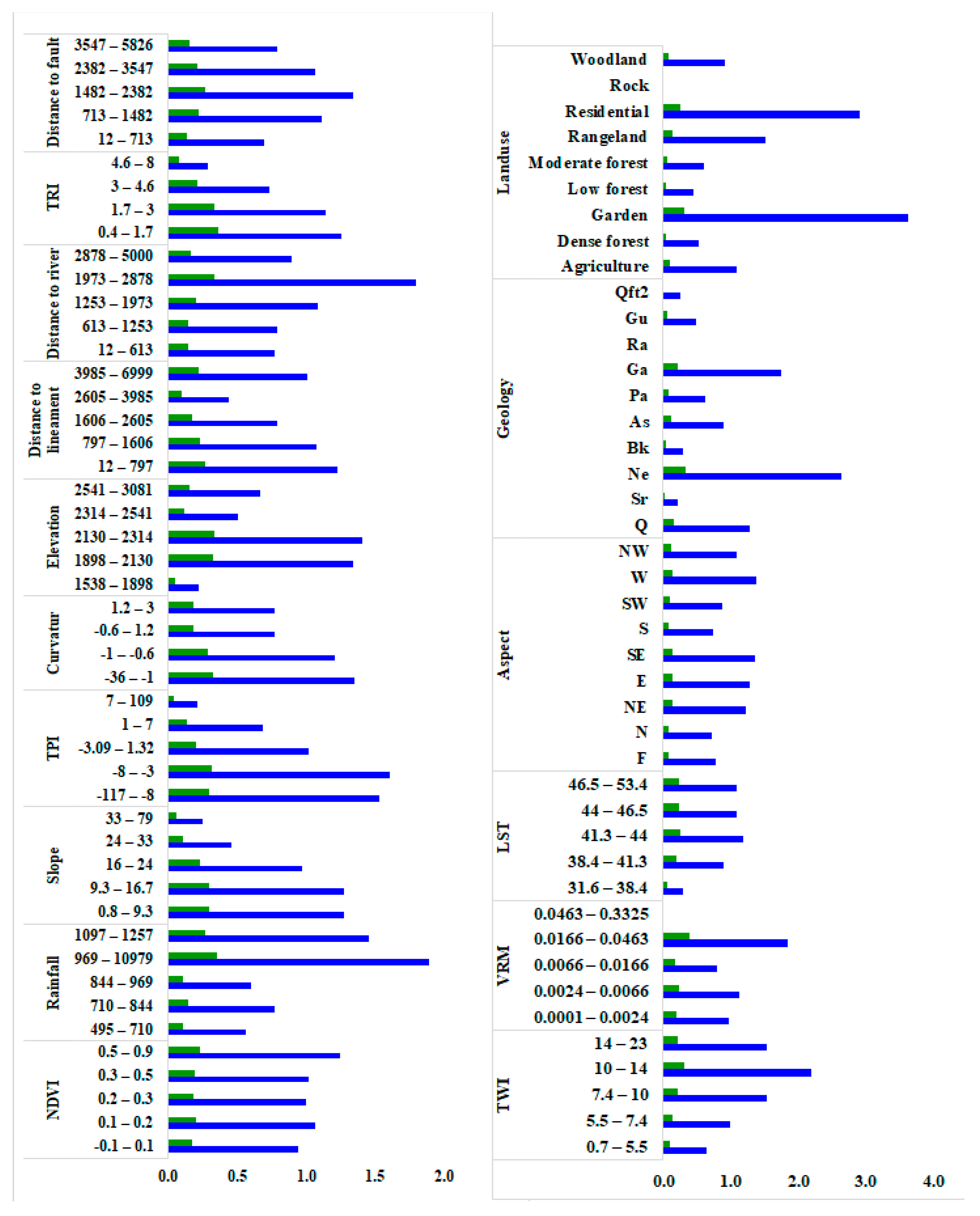
The set of spring locations of the calibration group was introduced as a dependent variable and the selected parameters (elevation classes, slope, etc.) were introduced as independent variables by the frequency ratio method. Using the frequency ratio technique, the probability of the presence of a spring in each class was calculated for all parameters. Comparative analyzes between the position of springs and environmental parameters affecting groundwater were performed using FR and entropy models, the results of which are shown in

Table 3. Spatial relationships between influence factors and spring locations.

Factor	Classes	Percentage of Domain	Percentage of Springs	FR	PD	Hj	Hjmax	Ij	Vj	W
NDVI	−0.15 to 0.14	44.17	41.67	0.94	0.18	2.3	2.3	0.003	0.003	0.002
	0.14–0.23	28.52	30.47	1.07	0.20
	0.23–0.33	17.21	17.19	1.00	0.19
	0.33–0.51	8.43	8.59	1.02	0.19
	0.51–0.93	1.67	2.08	1.24	0.24
Rainfall	495.95–710.25	13.89	7.81	0.56	0.11	2.1	2.3	0.074	0.078	0.049
	710.25–844.19	29.19	22.66	0.78	0.15
	844.19–969.20	25.28	15.10	0.60	0.11
	969.20–1097.19	19.46	36.72	1.89	0.36
	1097.19–1257.92	12.18	17.71	1.45	0.28
Slope	0.81–9.39	24.25	30.99	1.28	0.30	2.1	2.3	0.088	0.075	0.047
	9.39–16.73	27.10	34.64	1.28	0.30
	16.73–24.09	25.70	25.00	0.97	0.23
	24.09–33.41	17.69	8.07	0.46	0.11
	33.41–79.86	5.26	1.30	0.25	0.06
TPI	−117.17 to −8.40	5.12	7.81	1.53	0.30	2.1	2.3	0.097	0.098	0.061
	−8.40 to −3.09	19.76	31.77	1.61	0.32
	−3.09 to 1.32	37.99	38.54	1.01	0.20
	1.32–7.51	29.71	20.31	0.68	0.14
	7.51–109.20	7.43	1.56	0.21	0.04
Curvature	−36.48–−1.92	12.29	16.61	1.35	0.33	2.0	2.3	0.158	0.130	0.081
	−1.92 to −0.64	37.87	45.60	1.20	0.29
	−0.64 to 1.28	37.56	28.99	0.77	0.19
	1.28–3.2	11.39	8.79	0.77	0.19
	3.2–48	0.90	0.00	0.00	0.00
Elevation	1538–1898	11.81	2.60	0.22	0.05	2.1	2.3	0.106	0.088	0.055
	1898–2130	29.85	40.10	1.34	0.32
	2130–2314	29.19	41.15	1.41	0.34
	2314–2541	20.54	10.42	0.51	0.12
	2541–3081	8.62	5.73	0.66	0.16
Distance to lineament	12.5–797.75	33.97	41.67	1.23	0.27	2.3	2.3	0.031	0.028	0.017
	797.75–1606.43	29.96	32.29	1.08	0.24
	1606.43–2605.43	20.11	15.89	0.79	0.17
	2605.43–3985.63	10.54	4.69	0.44	0.10
	3985.63–6999.69	5.41	5.47	1.01	0.22
Distance to stream	12.5–613.64	30.51	23.70	0.78	0.15	2.2	2.3	0.035	0.038	0.023
	613.64–1253.555	27.31	21.61	0.79	0.15
	1253.55–1973.65	22.53	24.48	1.09	0.20
	1973.65–2878.42	14.10	25.26	1.79	0.34
	2878.42–5000	5.54	4.95	0.89	0.17
TRI	0.44–1.73	33.31	41.93	1.26	0.37	1.8	2.3	0.209	0.143	0.089
	1.73–3.08	33.09	37.76	1.14	0.33
	3.08–4.65	23.98	17.71	0.74	0.22
	4.65–8.02	8.97	2.60	0.29	0.08
	8.02–45.76	0.64	0.00	0.00	0.00
Fault	12.5–713.48	32.14	22.40	0.70	0.14	2.3	2.3	0.017	0.017	0.010
	713.48–1482.60	28.12	31.25	1.11	0.22
	1482.60–2382.52	20.82	27.86	1.34	0.27
	2382.52–3547.29	13.01	13.80	1.06	0.21
	3547.29–5826.93	5.92	4.69	0.79	0.16
TWI	0.73–5.54	41.61	27.08	0.65	0.09	2.2	2.3	0.047	0.065	0.040
	5.54–7.46	37.47	37.24	0.99	0.14
	7.46–10.17	13.42	20.57	1.53	0.22
	10.17–14.11	5.46	11.98	2.19	0.32
	14.11–23.11	2.04	3.13	1.54	0.22
VRM	0.0001–0.0024	73.17	70.83	0.97	0.20	1.9	2.3	0.172	0.164	0.102
	0.0024–0.0066	21.63	24.48	1.13	0.24
	0.0066–0.0166	4.59	3.65	0.79	0.17
	0.0166–0.0463	0.56	1.04	1.85	0.39
	0.0463–0.3325	0.05	0.00	0.00	0.00
LST	31.60–38.41	9.63	2.86	0.30	0.07	2.2	2.3	0.048	0.044	0.027
	38.41–41.39	18.70	16.67	0.89	0.20
	41.39–44.03	25.17	29.95	1.19	0.26
	44.03–46.59	27.41	29.69	1.08	0.24
	46.59–53.40	19.08	20.83	1.09	0.24
Aspect	Flat	13.75	10.68	0.78	0.08	2.8	3.2	0.128	0.134	0.084
	North	15.95	11.46	0.72	0.08
	Northeast	11.68	14.32	1.23	0.13
	East	9.13	11.72	1.28	0.14
	Southeast	10.47	14.32	1.37	0.14
	South	13.93	10.16	0.73	0.08
	Southwest	10.15	8.85	0.87	0.09
	West	7.32	10.16	1.39	0.15
	Northwest	7.63	8.33	1.09	0.12
Geology	Q	11.77	15.10	1.28	0.16	2.6	3.0	0.132	0.120	0.075
	Sr	6.15	1.30	0.21	0.03
	Ne	0.10	0.26	2.65	0.32
	Bk	1.84	0.52	0.28	0.03
	As	49.63	44.79	0.90	0.11
	Pa	10.78	6.77	0.63	0.08
	Ga	17.36	30.21	1.74	0.21
	Ra	0.26	0.00	0.00	0.00
	Gu	2.11	1.04	0.49	0.06
Land use	Agriculture	24.93	27.08	1.09	0.09	2.6	3.2	0.174	0.224	0.140
	Dense forest	1.49	0.78	0.52	0.05
	Garden	0.29	1.04	3.62	0.31
	Low forest	8.20	3.65	0.44	0.04
	Moderate forest	27.80	16.67	0.60	0.05
	Rangeland	27.37	41.41	1.51	0.13
	Residential	0.18	0.52	2.90	0.25
	Rock	0.00	0.00	0.00	0.00
	Woodland	9.74	8.85	0.91	0.08

and Figure 3. According to Table 3, the FR index values for the potential classes of each factor are shown in Figure 3. Then, the probability density (PD) and the final weight values of the entropy index of each factor were calculated based on FR.

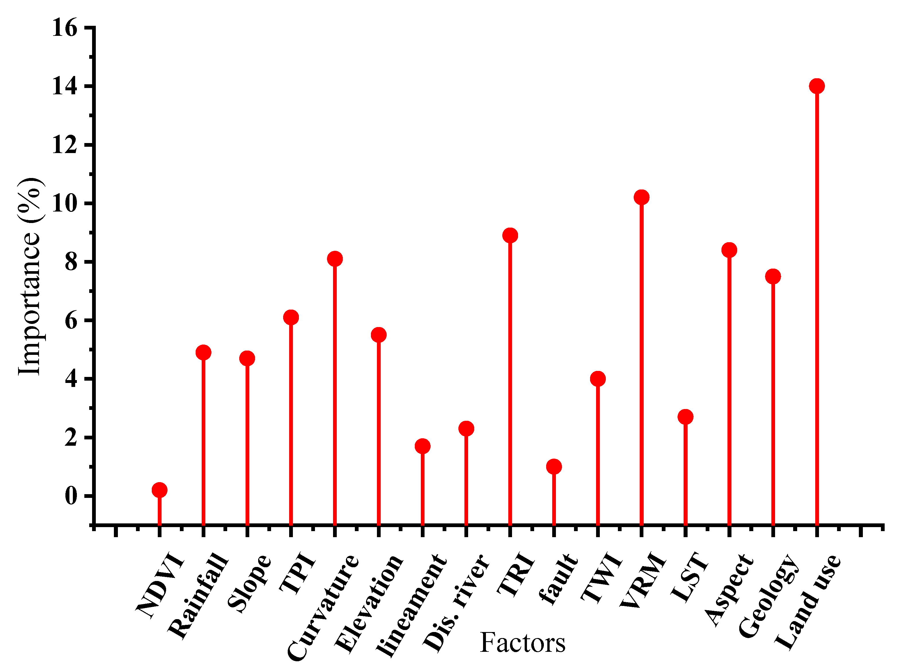
3.3. The Importance of FIGKRs

The variables that most influence the potential for springs (Figure 4) were land use, VRM, TRI, and aspect. NDVI, distance to nearest fault, LST, and distance to nearest stream were least important.

3.4. Karst Groundwater Potential Mapping (KGPM)

Karst groundwater potential was split into five classes (very low, low, moderate, high, and very high) using the natural break algorithm in ArcGIS 10.5 and then mapped (Figure 5).

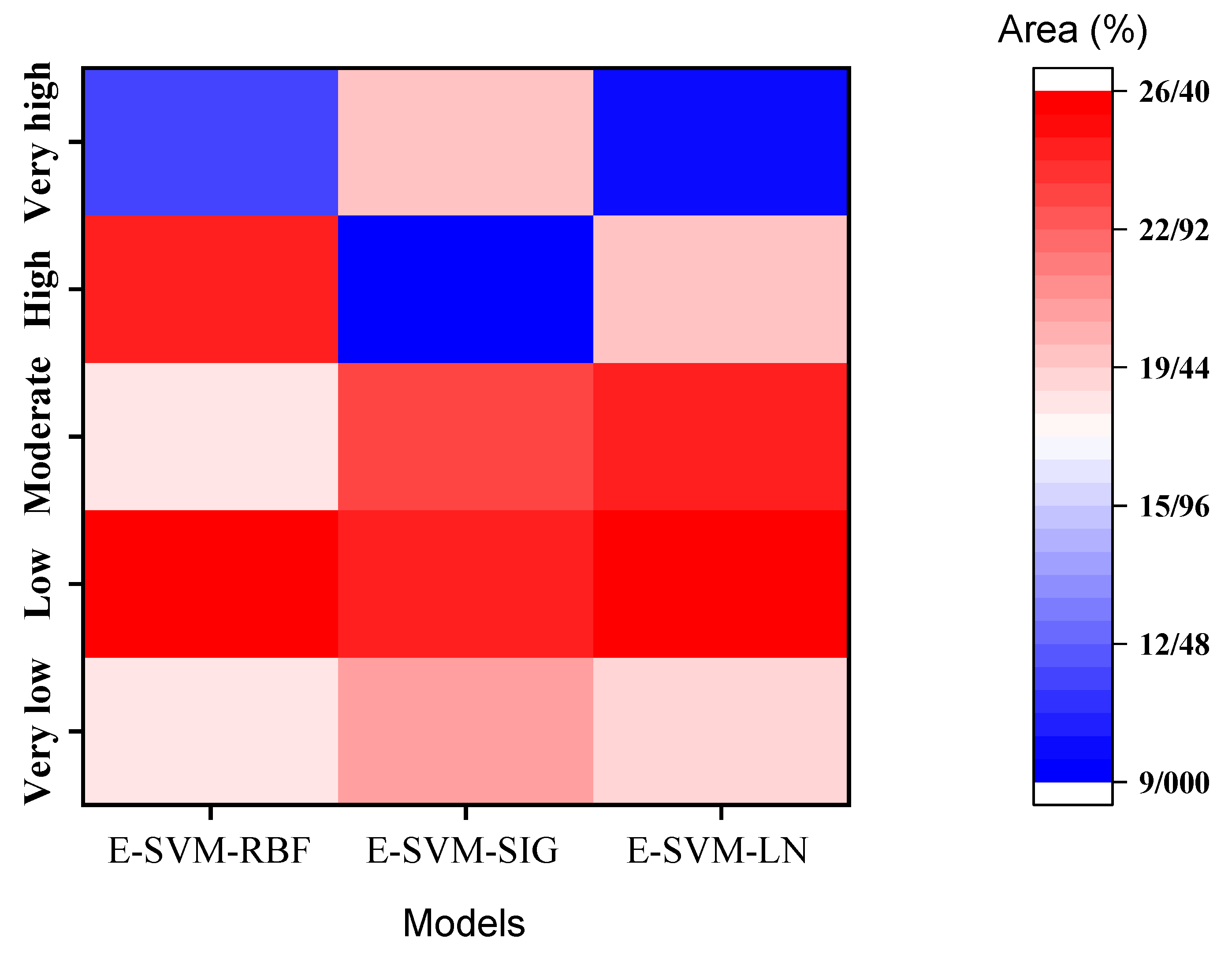
The results indicate that 11.6%, 20%, and 10% of the study area was classified as having very high potential by entropy-SVM-RBF, entropy-SVM-SIG, and entropy-SVM-LN (Figure 6). On the contrary, 18.5%, 21%, and 19% of the watershed was classified as having very low groundwater potential by the models (entropy-SVM-RBF, entropy-SVM-SIG, and entropy-SVM-LN).

3.5. Validation Analysis

The validation analysis showed that the entropy-SVM-RBF model (AUC = 0.911) was most accurate (Figure 7 and

Table 4. Statistical metrics used to evaluate the models’ performances.

	Models	AUC	SE	95% CI	PPV	NPV	Sensitivity	Specificity	Accuracy
Validating sample	E-SVM-RBF	0.911	0.0185	0.866–0.944	79.1	90.6	92.17	75.65	92.1
	E-SVM-SIG	0.820	0.0269	0.764–0.867	80.6	72.7	68.70	83.48	80.2
	E-SVM-LN	0.710	0.0330	0.647–0.768	65.8	67.3	68.70	64.35	68.4

). The standard error values of entropy-SVM-RBF were the smallest as well. The entropy-SVM-RBF produced the following metrics: SE = 0.0185, sensitivity = 92.17, specificity = 75.65, PPV = 79.1, NPV = 90.6, and accuracy = 92.1. This was the highest accuracy score among the models. Generally speaking, all three ensemble models achieved acceptable levels of accuracy for mapping karst groundwater potential. The results were validated both mathematically and empirically using of the field-determined locations of springs as truths. In fact, data-mining methods detect and match factors based on empirical evidence and this ultimately underpins predictions. Empirical data from field surveys and excavations (i.e., drilled wells) can also be used to validate modeling results after the fact.

4. Discussion

Karst formations may be the most important source for water supply in many parts of the world. A review of the literature showed that many studies have investigated groundwater potential using both machine learning and statistical models. Most of these studies focus on groundwater extracted from wells and rarely combine machine learning with statistical models to determine groundwater potential in watersheds in karst regions. This study determined karst groundwater potential using three new ensembles of statistical and machine learning algorithms—entropy-SVM-RBF, entropy-SVM-SIG and entropy-SVM-LN.

4.1. Machine Learning Algorithm Performance

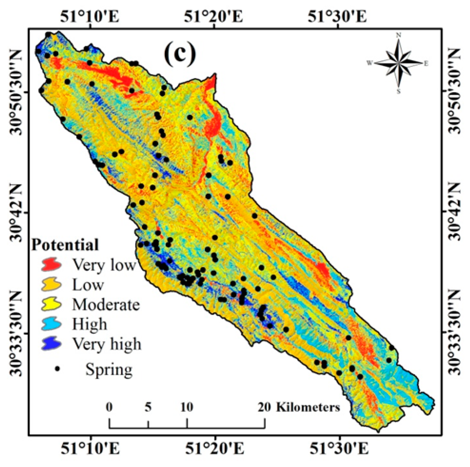
Analysis of spring potential classes showed that the areas of predicted lowest potential were largest and the areas of predicted highest potential were smallest for both the entropy-SVM-RBF and entropy-SVM-LN models. Moreover, geographically, the regions with the highest karst groundwater potential were predicted to be the southern and southeastern regions of the watershed. The results of the ROC analysis (Figure 7) indicated that the predictive performance of the entropy-SVM-RBF model was best and that it had the highest accuracy score at 0.911 as well. The entropy-SVM-SIG model’s accuracy was second best at 0.82, while entropy-SVM-LN had a 0.71 accuracy score. Examination of the assorted SVM kernels showed that their performances were affected by two variables—C and $\gamma$. These parameters were extracted using the grid-search technique. If the C and $\gamma$ variables were implemented using new optimization techniques, the performance of the kernels could be increased. Thus, it is recommended that future studies applying SVMs for groundwater potential prediction should use soft-computing optimization techniques to optimize the values of the kernel parameters. This demonstrates that use of SVM in combination with meta-heuristic algorithms and statistical models such as EBF and entropy can separately improve and enhance the prediction power and accuracy beyond the SVM, EBF, and entropy models. Abedini and Xu [49,50] also reported on the excellent results using SVM-RBF and SVM-entropy for other purposes. There was a significant difference between individual and ensemble models based on predictor performance. The average prediction rates based on AUC values revealed significant improvements. However, the results only pertain to these specific models; it is possible that the new ensembles could better predict groundwater potential map. It is suggested that the accuracy of other models be evaluated by other researchers. It would be better to compare other models in other studies and present their results.

4.2. Role of Factors in the Occurrence of Karst Springs

The relationships between the weights of the classes of the independent environmental factors and the Kabgian-dependent watershed springs variable were calculated (Table 3). The analysis of the importance of the factors affecting springs occurrence indicated that land use (14%) has the greatest impact on karst groundwater potential. This is followed by VRM (10%), TRI (9%), curvature (8%), aspect (8.5%), and geology (8%). As spring flow determines the type of land cover, land use determines the potential for groundwater. In that some land uses such as agriculture and residential development have extended into areas where springs previously existed, we can see the effect of land use on subsurface water. On the contrary, the extent and density of vegetation (especially where tree cover is limited) in many karst formations and in regions of high elevation can accentuate the influence of both land cover and land use.

A factor that has not often been used in previous studies and that was identified in this study as important is the VRM. This study revealed a greater importance of geological and geomorphological factors in the development and formation of karst springs. Unlike in non-karst regions, faults and lineaments have little influence on groundwater potential in karst zones. In fact, faulted and fractured areas in karst regions often serve as recharge zones, and springs are found at the outlet of aquifers. In past studies, factors such as faults and fault-related features have been identified as important for the creation of springs, but in this watershed, faults are apparently not very important. Moreover, in previous studies, the distance from the nearest river was also found to be important, but in this study, it was not. This contradicts the findings in other studies [34,51]. The lower importance of distance from a river is, in part, due to the hydrology of karst. Aquifers do not necessarily follow surface streams and rivers. In contrast, [30,31,32,33,34,35,36,37,38,39,40,41,42,43,44,45,46,47,48,49,50,51,52,53,54,55] identified land use and land cover, curvature, and lithology as most important to the formation and development of springs in this region of karst. Since the land surface temperature in areas near springs was expected to be cooler than those without springs due to the influence of flowing water on the surface temperature, we used an LST index. LST had a significance of only 3% on KGP, which was somewhat higher than distance from the nearest fault, distance from the nearest lineament, distance from the nearest river, and NDVI. NDVI had the least influence on KGP, perhaps due to the lack of contact between vegetation and aquifers in the region. Though karst aquifers are obviously saturated and have abundant water to support vegetation, they tend to be deep below the surface, beyond the root zones that absorb water for plants.

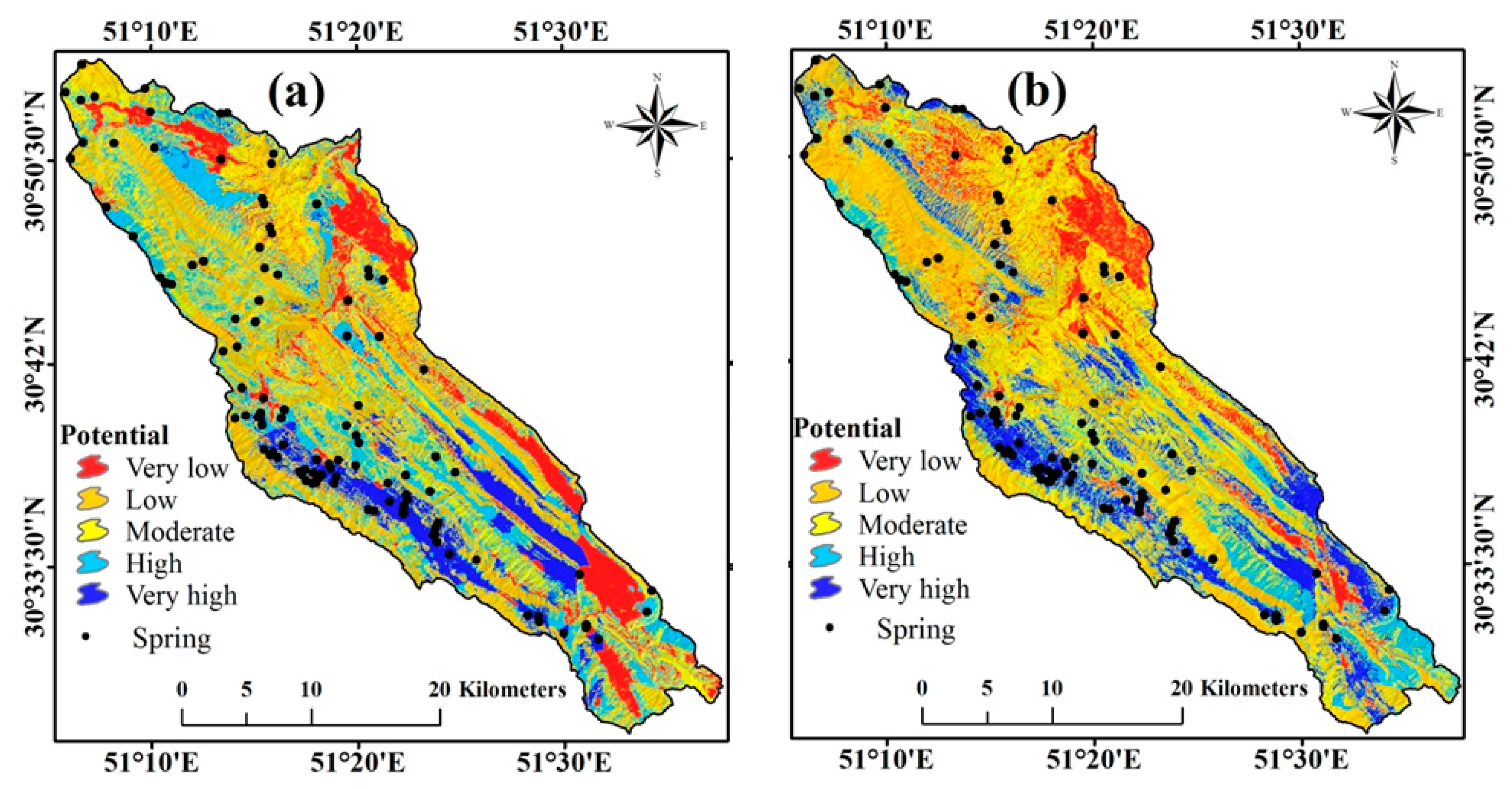
Various environmental factors affect the presence of springs in an area. Springs will appear at points where different conditions are suitable. In general, the higher the density of springs in an area, the better the environmental conditions for springs and vice versa. Therefore, the existence of only one spring does not represent appropriate conditions for spring development; numerous springs must be present for this to be the case. Individual springs are found in low-potential areas due to unknown and idiosyncratic conditions. It may be very difficult and expensive to determine these factors for the purpose of developing maps of spring potential. However, as shown in Figure 5, there are no springs in areas with very low potential (red areas). On the contrary, there are no springs in some areas with very high potential (blue areas); this state can be due to two reasons: A statistical gap and lack of accurate ground data related to spring distribution of springs, or the absence of specific conditions during a specific time frame that causes the absence or disappearance of springs. What is important in machine learning models is to locate these areas so that despite a lack of accurate information and data, it is still possible to map spring potential throughout the study area.

5. Conclusions

This study evaluated the ability of data-mining models to predict areas of groundwater potential in a karst region. Machine learning and statistical models were combined to create three models: Entropy-SVM-LN, entropy-SVM-SG, and entropy-SVM-RBF. Sixteen conditioning factors were measured to produce a database for the watershed, and 384 springs were used as locations of known aquifer presence. The predictions of the three models demonstrated that they were effective at determining the potential for groundwater throughout the watershed. The results showed that the factors that promote the presence of springs in the region are different from the factors that are known to predict the presence of springs in non-karst regions. Measures of precipitation and geologic formation may be the most important influences on spring formation in non-karst areas, but in karst regions, geomorphometric variables, such as VRM and TRI, and surface curvature are the most important factors influencing groundwater potential. Land use and land cover have significant relationships with groundwater in karst zones. Faults and lineaments serve as locations of recharge for aquifers in karst regions and springs may appear at great distances from them due to hydraulic slopes. These features in non-karst regions can indicate the locations of groundwater resources because flows through porous media with non-Darcy conditions are directly related to faults and lineaments. In karst regions, groundwater resources are unrelated to either LST indices that indicate hot or cold spots or NDVI. There are many models and algorithms that can be used to map groundwater potential, but this study compared individual and ensemble results of the entropy statistical model and SVM machine learning algorithms to map groundwater potential. The results only pertain to these specific models. It is possible that the new ensembles could better predict groundwater potential maps. It is suggested that the accuracy of other models be evaluated by other researchers. It would be better to compare other models in other studies and present those results. Finally, we suggest that geophysical field methods be used to validate results to accurately assess groundwater potential in the karst landscape of the study area.

References

- Kumar, A.; Pandey, A.C. Geoinformatics Based Groundwater Potential Assessment in Hard Rock Terrain of Ranchi Urban Environment, Jharkhand State (India) Using MCDM—AHP Techniques. Groundw. Sustain. Dev. 2016, 2, 27–41. [Google Scholar] [CrossRef]
- Amin, M.M.; Veith, T.L.; Collick, A.S.; Karsten, H.D.; Buda, A.R. Simulating Hydrological and Nonpoint Source Pollution Processes in a Karst Watershed: A Variable Source Area Hydrology Model Evaluation. Agric. Water Manag. 2017, 180, 212–223. [Google Scholar] [CrossRef] [Green Version]
- Chen, W.; Pourghasemi, H.R.; Naghibi, S.A. A Comparative Study of Landslide Susceptibility Maps Produced Using Support Vector Machine with Different Kernel Functions and Entropy Data Mining Models in China. Bull. Eng. Geol. Environ. 2018, 77, 647–664. [Google Scholar] [CrossRef]
- Stevanović, Z. Karst waters in potable water supply: A global scale overview. Environ. Earth Sci. 2019, 78, 1–12. [Google Scholar] [CrossRef]
- Andreo, B.; Vías, J.; Durán, J.J.; Jiménez, P.; López-Geta, J.A.; Carrasco, F. Methodology for Groundwater Recharge Assessment in Carbonate Aquifers: Application to Pilot Sites in Southern Spain. Hydrogeol. J. 2008, 16, 911–925. [Google Scholar] [CrossRef]
- De Giglio, O.; Caggiano, G.; Apollonio, F.; Marzella, A.; Brigida, S.; Ranieri, E.; Lucentini, L.; Uricchio, V.F.; Montagna, M.T. The aquifer recharge: An overview of the legislative and planning aspect. Ann Ig 2018, 30, 34–43. [Google Scholar] [PubMed]
- Jebreen, H.; Banning, A.; Wohnlich, S. Karst Groundwater Resources: Problems, Management, and Sustainability, an Example from a Carbonate Aquifer in Palestine. AGU Fall Meet. Abstr. 2018, 2018, H53L-1744. [Google Scholar]
- Stevanović, Z.; Marinović, V.; Krstajić, J. CC-PESTO: A Novel GIS-Based Method for Assessing the Vulnerability of Karst Groundwater Resources to the Effects of Climate Change. Hydrogeol. J. 2020, 29, 159–178. [Google Scholar] [CrossRef]
- Kresic, N. Groundwater Resources; McGraw-Hili: New York, NY, USA, 2009. [Google Scholar]
- Manap, M.A.; Nampak, H.; Pradhan, B.; Lee, S.; Sulaiman, W.N.A.; Ramli, M.F. Application of Probabilistic-Based Frequency Ratio Model in Groundwater Potential Mapping Using Remote Sensing Data and GIS. Arab. J. Geosci. 2014, 7, 711–724. [Google Scholar] [CrossRef]
- Reberski, J.L.; Rubinić, J.; Terzić, J.; Radišić, M. Climate Change Impacts on Groundwater Resources in the Coastal Karstic Adriatic Area: A Case Study from the Dinaric Karst. Nat. Resour. Res. 2020, 29, 1975–1988. [Google Scholar] [CrossRef]
- Avand, M.; Janizadeh, S.; Bui, D.T.; Pham, V.H.; Ngo, P.T.T.; Nhu, V.-H. A Tree-Based Intelligence Ensemble Approach for Spatial Prediction of Potential Groundwater. Int. J. Digit. Earth 2020, 13, 1408–1429. [Google Scholar] [CrossRef]
- Moradi, H.; Avand, M.T.; Janizadeh, S. Landslide Susceptibility Survey Using Modeling Methods. In Spatial Modeling in GIS and R for Earth and Environmental Sciences; Pourghasemi, H.R., Gokceoglu, C., Eds.; Elsevier: Amsterdam, The Netherlands, 2019; pp. 259–276. [Google Scholar]
- Pham, B.T.; Phong, T.V.; Avand, M.; Al-Ansari, N.; Singh, S.K.; Le, H.V.; Prakash, I. Improving Voting Feature Intervals for Spatial Prediction of Landslides. Math. Probl. Eng. 2020, 2020, 4310791. [Google Scholar] [CrossRef]
- Chowdhury, A.; Jha, M.K.; Chowdary, V.M. Delineation of Groundwater Recharge Zones and Identification of Artificial Recharge Sites in West Medinipur District, West Bengal, Using RS, GIS and MCDM Techniques. Environ. Earth Sci. 2010, 59, 1209–1222. [Google Scholar] [CrossRef]
- Abd Manap, M.; Sulaiman, W.N.A.; Ramli, M.F.; Pradhan, B.; Surip, N. A Knowledge-Driven GIS Modeling Technique for Groundwater Potential Mapping at the Upper Langat Basin, Malaysia. Arab. J. Geosci. 2013, 6, 1621–1637. [Google Scholar] [CrossRef]
- Lee, S.; Hong, S.M.; Jung, H.S. GIS-Based Groundwater Potential Mapping Using Artificial Neural Network and Support Vector Machine Models: The Case of Boryeong City in Korea. Geocarto Int. 2018, 33, 847–861. [Google Scholar] [CrossRef]
- Naghibi, S.A.; Pourghasemi, H.R.; Dixon, B. GIS-Based Groundwater Potential Mapping Using Boosted Regression Tree, Classification and Regression Tree, and Random Forest Machine Learning Models in Iran. Environ. Monit. Assess. 2016, 188, 44. [Google Scholar] [CrossRef] [PubMed]
- Guru, B.; Seshan, K.; Bera, S. Frequency Ratio Model for Groundwater Potential Mapping and Its Sustainable Management in Cold Desert, India. J. King Saud Univ.-Sci. 2017, 29, 333–347. [Google Scholar] [CrossRef] [Green Version]
- Kordestani, M.D.; Naghibi, S.A.; Hashemi, H.; Ahmadi, K.; Kalantar, B.; Pradhan, B. Groundwater Potential Mapping Using a Novel Data-Mining Ensemble Model. Hydrogeol. J. 2019, 27, 211–224. [Google Scholar] [CrossRef] [Green Version]
- Miraki, S.; Zanganeh, S.H.; Chapi, K.; Singh, V.P.; Shirzadi, A.; Shahabi, H.; Pham, B.T. Mapping Groundwater Potential Using a Novel Hybrid Intelligence Approach. Water Resour. Manag. 2019, 33, 281–302. [Google Scholar] [CrossRef]
- Nguyen, P.T.; Ha, D.H.; Avand, M.; Jaafari, A.; Nguyen, H.D.; Al-Ansari, N.; Van Phong, T.; Sharma, R.; Kumar, R.; Le, H.V.; et al. Soft Computing Ensemble Models Based on Logistic Regression for Groundwater Potential Mapping. Appl. Sci. 2020, 10, 2469. [Google Scholar] [CrossRef] [Green Version]
- Termeh, S.V.R.; Khosravi, K.; Sartaj, M.; Keesstra, S.D.; Tsai, F.T.C.; Dijksma, R.; Pham, B.T. Optimization of an Adaptive Neuro-Fuzzy Inference System for Groundwater Potential Mapping. Hydrogeol. J. 2019, 27, 2511–2534. [Google Scholar] [CrossRef]
- Gilli, E. Deep speleological salt contamination in Mediterranean karst aquifers: Perspectives for water supply. Environ. Earth Sci. 2015, 74, 101–113. [Google Scholar] [CrossRef]
- Díaz-Alcaide, S.; Martínez-Santos, P. Mapping fecal pollution in rural groundwater supplies by means of artificial intelligence classifiers. J. Hydrol. 2019, 577, 124006. [Google Scholar] [CrossRef]
- Rahmati, O.; Avand, M.; Yariyan, P.; Tiefenbacher, J.P.; Azareh, A.; Bui, D.T. Assessment of Gini, Entropy, and Ratio Based Classification Trees for Groundwater Potential Modeling and Prediction. Geocarto Int. 2020, 34, 1–18. [Google Scholar]
- Beverly, C.; Hocking, M. Predicting Groundwater Response Times and Catchment Impacts from Land Use Change. Australas. J. Water Resour. 2012, 16, 29–47. [Google Scholar] [CrossRef]
- Ozdemir, A. GIS-Based Groundwater Spring Potential Mapping in the Sultan Mountains (Konya, Turkey) Using Frequency Ratio, Weights of Evidence and Logistic Regression Methods and Their Comparison. J. Hydrol. 2011, 411, 290–308. [Google Scholar] [CrossRef]
- Pham, B.T.; Jaafari, A.; Prakash, I.; Singh, S.K.; Quoc, N.K.; Bui, D.T. Hybrid Computational Intelligence Models for Groundwater Potential Mapping. Catena 2019, 182, 104101. [Google Scholar] [CrossRef]
- Ozdemir, A. Using a Binary Logistic Regression Method and GIS for Evaluating and Mapping the Groundwater Spring Potential in the Sultan Mountains (Aksehir, Turkey). J. Hydrol. 2011, 405, 123–136. [Google Scholar] [CrossRef]
- Arulbalaji, P.; Padmalal, D.; Sreelash, K. GIS and AHP Techniques Based Delineation of Groundwater Potential Zones: A Case Study from Southern Western Ghats, India. Sci. Rep. 2019, 9, 1–17. [Google Scholar] [CrossRef]
- Dar, I.A.; Sankar, K.; Dar, M.A. Remote Sensing Technology and Geographic Information System Modeling: An Integrated Approach towards the Mapping of Groundwater Potential Zones in Hardrock Terrain, Mamundiyar Basin. J. Hydrol. 2010, 394, 285–295. [Google Scholar] [CrossRef]
- Naghibi, S.A.; Vafakhah, M.; Hashemi, H.; Pradhan, B.; Alavi, S.J. Groundwater Augmentation through the Site Selection of Floodwater Spreading Using a Data Mining Approach (Case Study: Mashhad Plain, Iran). Water 2018, 10, 1405. [Google Scholar] [CrossRef] [Green Version]
- Rahmati, O.; Naghibi, S.A.; Shahabi, H.; Bui, D.T.; Pradhan, B.; Azareh, A.; Rafiei-Sardooi, E.; Samani, A.N.; Melesse, A.M. Groundwater Spring Potential Modelling: Comprising the Capability and Robustness of Three Different Modeling Approaches. J. Hydrol. 2018, 565, 248–261. [Google Scholar] [CrossRef]
- Scanlon, B.R.; Reedy, R.C.; Stonestrom, D.A.; Prudic, D.E.; Dennehy, K.F. Impact of Land Use and Land Cover Change on Groundwater Recharge and Quality in the Southwestern US. Glob. Chang. Biol. 2005, 11, 1577–1593. [Google Scholar] [CrossRef]
- De Reu, J.; Bourgeois, J.; Bats, M.; Zwertvaegher, A.; Gelorini, V.; De Smedt, P.; Chu, W.; Antrop, M.; De Maeyer, P.; Finke, P.; et al. Application of the Topographic Position Index to Heterogeneous Landscapes. Geomorphology 2013, 186, 39–49. [Google Scholar] [CrossRef]
- Rizeei, H.M.; Pradhan, B.; Saharkhiz, M.A.; Lee, S. Groundwater Aquifer Potential Modeling Using an Ensemble Multi-Adoptive Boosting Logistic Regression Technique. J. Hydrol. 2019, 579, 124172. [Google Scholar] [CrossRef]
- Al-Abadi, A.M.; Shahid, S. A Comparison between Index of Entropy and Catastrophe Theory Methods for Mapping Groundwater Potential in an Arid Region. Environ. Monit. Assess. 2015, 187, 576. [Google Scholar] [CrossRef] [Green Version]
- Naghibi, S.A.; Pourghasemi, H.R.; Pourtaghi, Z.S.; Rezaei, A. Groundwater Qanat Potential Mapping Using Frequency Ratio and Shannon’s Entropy Models in the Moghan Watershed, Iran. Earth Sci. Inform. 2015, 8, 171–186. [Google Scholar] [CrossRef]
- Vapnik, V.; Guyon, I.; Hastie, T. Support Vector Machines. Mach. Learn. 1995, 20, 273–297. [Google Scholar]
- Chapelle, O.; Vapnik, V.; Bousquet, O.; Mukherjee, S. Choosing Multiple Parameters for Support Vector Machines. Mach. Learn. 2002, 46, 131–159. [Google Scholar] [CrossRef]
- Park, S.; Choi, C.; Kim, B.; Kim, J. Landslide Susceptibility Mapping Using Frequency Ratio, Analytic Hierarchy Process, Logistic Regression, and Artificial Neural Network Methods at the Inje Area, Korea. Environ. Earth Sci. 2013, 68, 1443–1464. [Google Scholar] [CrossRef]
- Razandi, Y.; Pourghasemi, H.R.; Neisani, N.S.; Rahmati, O. Application of Analytical Hierarchy Process, Frequency Ratio, and Certainty Factor Models for Groundwater Potential Mapping Using GIS. Earth Sci. Inform. 2015, 8, 867–883. [Google Scholar] [CrossRef]
- Pham, B.T.; Jaafari, A.; Avand, M.; Al-Ansari, N.; Dinh Du, T.; Yen, H.P.H.; Phong, T.V.; Nguyen, D.H.; Le, H.V.; Mafi-Gholami, D.; et al. Performance evaluation of machine learning methods for forest fire modeling and prediction. Symmetry 2020, 12, 1022. [Google Scholar] [CrossRef]
- Yousefi, S.; Pourghasemi, H.R.; Avand, M.; Janizadeh, S.; Tavangar, S.; Santosh, M. Assessment of Land Degradation Using Machine-Learning Techniques: A Case of Declining Rangelands. Land Degrad. Dev. 2020, 32, 1452–1466. [Google Scholar] [CrossRef]
- Yariyan, P.; Avand, M.; Abbaspour, R.A.; Torabi Haghighi, A.; Costache, R.; Ghorbanzadeh, O.; Janizadeh, S.; Blaschke, T. Flood susceptibility mapping using an improved analytic network process with statistical models. Geomatics. Nat. Hazards Risk 2020, 11, 2282–2314. [Google Scholar] [CrossRef]
- Avand, M.; Moradi, H.R.; Ramazanzadeh Lasboyee, M. Spatial Prediction of Future Flood Risk: An Approach to the Effects of Climate Change. Geosciences 2021, 11, 25. [Google Scholar] [CrossRef]
- Phong, T.V.; Pham, B.T.; Trinh, P.T.; Ly, H.B.; Vu, Q.H.; Ho, L.S.; Le, H.V.; Phong, L.H.; Avand, M.; Prakash, I. Groundwater Potential Mapping Using GIS-Based Hybrid Artificial Intelligence Methods. Groundwater 2021, 59, 745–760. [Google Scholar] [CrossRef]
- Abedini, M.; Ghasemian, B.; Shirzadi, A.; Bui, D.T. A Comparative Study of Support Vector Machine and Logistic Model Tree Classifiers for Shallow Landslide Susceptibility Modeling. Environ. Earth Sci. 2019, 78, 560. [Google Scholar] [CrossRef]
- Xu, F.; Peter, W.T. A Method Combining Refined Composite Multiscale Fuzzy Entropy with PSO-SVM for Roller Bearing Fault Diagnosis. J. Cent. South Univ. 2019, 26, 2404–2417. [Google Scholar] [CrossRef]
- Hou, E.; Wang, J.; Chen, W. A Comparative Study on Groundwater Spring Potential Analysis Based on Statistical Index, Index of Entropy and Certainty Factors Models. Geocarto Int. 2018, 33, 754–769. [Google Scholar] [CrossRef]
- Zelenakova, M.; Repel, A.; Vranayova, Z.; Kaposztasova, D.; Abd-Elhamid, H.F. Impact of land use changes on surface runoff in urban areas-Case study of Myslavsky Creek Basin in Slovakia. Acta Montan. Slovaca 2019, 24, 129–139. [Google Scholar]
- Zelenakova, M.; Hudakova, G.; Tometz, L.; Hlavata, H. Investigation of Rainwater Infiltration with Emphasis on Hydro-geological as well as Hydrological Conditions. In Proceedings of the 10th International Conference on Environmental Engineering. ICEE (10th ICEE), Vilnius Gediminas Technical University, Vilnius, Lithuania, 27–28 April 2017. [Google Scholar]
- Naghibi, S.A.; Dolatkordestani, M.; Rezaei, A.; Amouzegari, P.; Heravi, M.T.; Kalantar, B.; Pradhan, B. Application of Rotation Forest with Decision Trees as Base Classifier and a Novel Ensemble Model in Spatial Modeling of Groundwater Potential. Environ. Monit. Assess. 2019, 191, 1–20. [Google Scholar] [CrossRef] [PubMed]
- Naghibi, S.A.; Dashtpagerdi, M.M. Evaluation of Four Supervised Learning Methods for Groundwater Spring Potential Mapping in Khalkhal Region (Iran) Using GIS-Based Features. Hydrogeol. J. 2017, 25, 169–189. [Google Scholar] [CrossRef]
Figure 1.
Location of the Kabgian watershed in Iran.
Figure 2.
Factors influencing karst groundwater potential: (A) Elevation, (B) aspect, (C) curvature, (D) distance to lineament, (E) distance from stream, (F) distance to fault, (G) geology, (H) land use, (I) LST, (J) NDVI, (K) rainfall, (L) slope, (M) TWI, (N) TPI, (O) VTR, and (P) TRI.
Figure 3.
FR values for the FIGKR classes.
Figure 4.
Variable importance analysis.
Figure 5.
Karst groundwater potential maps generated by (a) entropy-SVM-RBF, (b) entropy-SVM-SIG, and (c) entropy-SVM-LN.
Figure 6.
Percentage of karst groundwater potential classes in the study area.
Figure 7.
Evaluation the accuracies of the models’ karst groundwater potential mapping using the ROC curve.