Improvement of Downstream Flow by Modifying SWAT Reservoir Operation Considering Irrigation Water and Environmental Flow from Agricultural Reservoirs in South Korea

Abstract

This study aims to develop a reservoir operation rule adding downstream environmental flow release (EFR) to the exclusive use of irrigation water supply (IWS) from agricultural reservoirs through canals to rice paddy areas. A reservoir operation option was added in the Soil and Water Assessment Tool (SWAT) to handle both EFR and IWS. For a 366.5 km² watershed including three agricultural reservoirs and a rice paddy irrigation area of 4744.7 ha, the SWAT was calibrated and validated using 21 years (1998–2018) of daily reservoir water levels and downstream flow data at Gongdo (GD) station. For reservoir water level and streamflow, the average root means square error (RMSE) ranged from 19.70 mm to 19.54 mm, and the coefficient of determination (R²) and Nash–Sutcliffe efficiency (NSE) had no effect on the improved SWAT. By applying the new reservoir option, the EFR amount for a day was controlled by keeping the reservoir water level up in order to ensure that the IWS was definitely satisfied in any case. The downstream mean wet streamflow (Q95) decreased to 5.70 m³/sec from 5.71 m³/sec and the mean minimum flow (Q355) increased to 1.05 m³/sec from 0.94 m³/sec. Through the development of a SWAT reservoir operation module that satisfies multiple water supply needs such as IWR and EFR, it is possible to manage agricultural water in the irrigation period and control the environmental flow in non-irrigation periods. This study provides useful information to evaluate and understand the future impacts of various changes in climate and environmental flows at other sites.

1. Introduction

Through industrial development, groundwater resources have been built in rural areas through new land development, groundwater use and river renovation, and this flow has changed water availability due to river regulation in more than half of the world’s rivers [1]. However, due to such development small and medium-sized streams face severe stream drying phenomena because of the distortion of the hydrological circulation system [2]. Agricultural reservoirs in small river basins located upstream of rural areas have been severely dried. The hydrological circulation process has been artificially cut off because of the priority placed on the supply of agricultural water. Environmental flow has been introduced to recover the hydrological cycle distorted by environmental changes such as urbanization, groundwater use, and river cover. Agricultural areas in South Korea have been exposed to severe conditions by long-term drought during the past decade, and the severely abnormal drought of 2013–2017 has resulted in water shortages and insufficient flow to maintain aquatic ecosystems. To mitigate the stream drying phenomena, including the water quantity and water quality of small and medium-sized streams, environmental flow release (EFR) is necessary.

Water can be allocated to environmental needs as an environmental flow with regulated patterns. Two major paradigms are well known for EFR regimes in altered rivers: (1) the natural flow regime and (2) the expected regime. In regions with high seasonal agricultural water demand, the release of EFR from the reservoirs to the lakes is a challenge when water is used for irrigation shortly after its release [3,4,5,6,7,8,9]. There are more than 200 methods used worldwide for the calculation of EFR, and these methodologies are divided into four broad categories: hydrological approaches, hydraulic rating, habitat simulation, and holistic methods [10,11]. However, available data for small and medium-sized streams are limited, and only rivers that are recognized for their importance such as national rivers and regional primary rivers are considered in South Korea. Therefore, an accurate calculation formula is not available, and most EFRs in small and medium-sized streams have a role as agricultural reservoirs [11,12,13].

In South Korea, 17,649 agricultural reservoirs have been developed to secure water for agricultural activities. The amount of agricultural water in South Korea is 15.2 billion m³, approximately 61% of the available water resources [12]. As of 2014, 80.8% of the paddy area was supplied by agricultural facilities, of which 59.9% was supplied by reservoirs [14]. In 2009, as the need for EFR increased, the Korea Rural Community Corporation (KRC) implemented an agricultural reservoir heightened embankment project to increase the capacity of 110 agricultural reservoirs located on middle and upper reaches. The agricultural reservoir heightened embankment project smoothly supplied irrigation water requirements (IWR) and stream maintenance in agricultural areas, and reinforced reservoirs vulnerable to disaster [12,14,15]. However, in order to supply EFR, the water level in the reservoir from mid-April to mid-May—which is the time of IWR for the following year—should be considered from the time when agricultural activities conclude. Therefore, it is necessary to build an operation rule for agricultural reservoirs that satisfies both IWR and EFR, unlike the existing rule [16].

Various studies in South Korea on water requirement operations have been performed using other models or by updating the HOMWRS (Hydrological Operation Model for Water Resources System) model, which was developed for single reservoir design [17,18,19,20]. Since the above model was developed individually, it is difficult for other researchers to link it and integrate information. Because of the advantage of using the semi-distributed runoff model, evaluation of various scenarios can be used, and research on the development of agricultural reservoir management and operation techniques is ongoing based on the SWAT model [21,22]. Cau and Paniconi [23] studied irrigation applications using optimum irrigation management, where the irrigation supply was specified by the water requirements of crops for SWAT. Piniewski et al. [24] assessed changes in the environmental flow regime of the reservoir system caused by climate change using SWAT and a continental model of water availability. Although these studies do not consider a combination of IWR and EFR, many studies have attempted to optimize reservoir operation by combining SWAT and a probabilistic algorithm [25,26,27]. Therefore, if a SWAT model capable of simulating IWR and EFR is developed, it can quickly establish the optimized reservoir operating rule accordingly.

In this study, the SWAT was improved to consider both the IWR and EFR of agricultural reservoirs simultaneously. The reservoir operation rules were estimated by considering the IWR and EFR in the agricultural reservoir according to the restricted water level. First, the SWAT was calibrated and validated, and the resulting difference of SWAT and improved SWAT was confirmed. Second, the reservoir storage rate change was investigated when considering IWR and EFR in the improved SWAT. Third, we tried to estimate the reservoir operation rules by checking the downstream flow rate change (Figure 1).

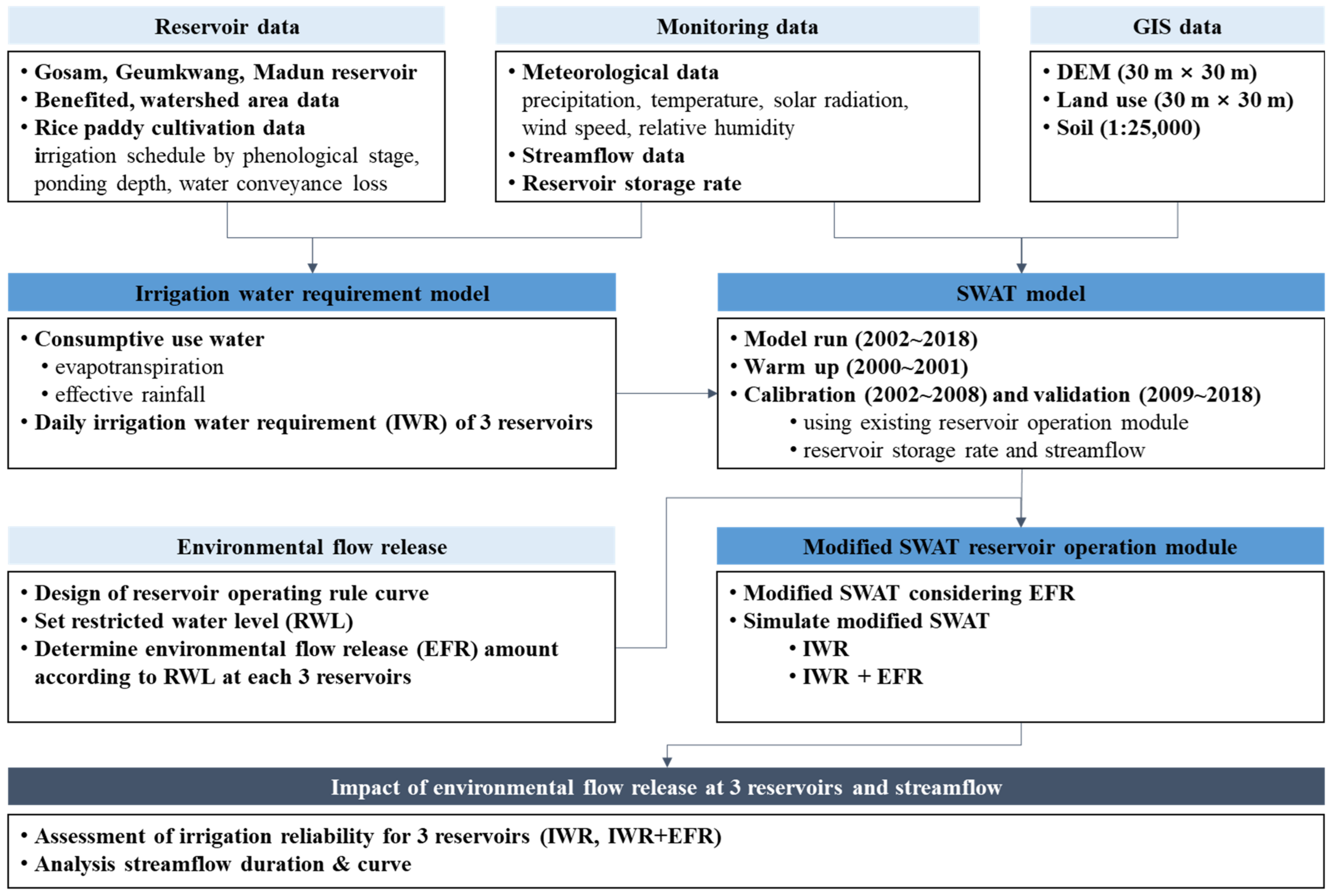
2. Irrigation Water and Environmental Flow Module Development

2.1. Irrigation Water Requirement Calculation of Paddy Rice

The irrigation water requirement model (IWRM) was developed to calculate the daily-basis IWR in rice paddy fields and use the input data for the improved SWAT reservoir module. The IWRM calculates the daily paddy rice consumption of water, and the reservoir release amount based on daily weather conditions, evapotranspiration, percolation with soil information, canal water delivery, and management of water loss. The model allows the management of irrigation scheduling for a determined ponding depth during the rice cultivation period. The model considers sufficient rainfall and evaluates the irrigation practices of farmers, and manages reservoir water levels in the case of normal and water deficit periods during drought with partial irrigation conditions.

The water balance method is used to calculate irrigation schedules in IWRM, which means that the incoming and outgoing (

Table A1. The input and output datasets of IWRM.

Data	Input	Output
Climatic	Location of weather station, Daily rainfall (mm), Daily air temperature (°C), Daily relative humidity (%), Daily sunshine hour (hr), Daily wind speed (m/s)	Reference ET (ET0, m3) Crop ET (ETc, m3) Consumptive water use (m3) Ponding depth (mm) Effective rainfall (m3) Net duty of water (m3) Gross duty of water (m3)
Crop (rice)	$\mathrm{Percent} \mathrm{area} \mathrm{of} \mathrm{rice} \mathrm{nursery} \mathrm{bed} (\%), \mathrm{Water} \mathrm{for} \mathrm{rice} \mathrm{seeding} \left(\mathrm{mm}\right), \mathrm{Water} \mathrm{for} \mathrm{rice} \mathrm{transplanting} \left(\mathrm{mm}\right), \mathrm{Crop} \mathrm{coefficient} \left(K_c\right)$ for ET, maximum and minimum ponding depths (mm)
Soil	Daily infiltration of paddy field (mm)
Irrigation	Irrigated area (ha), Irrigation schedule (seeding, planting, and harvesting dates), Water conveyance loss of irrigation canal (%), Water management loss of irrigation facilities (%)

) water flows from the rice paddy field are monitored. The calculation procedures used in IWRM are based on the Food and Agriculture Organization of the United Nations (FAO) publication of the Irrigation and Drainage Series, namely, No. 56 Crop Evapotranspiration-Guidelines for computing crop water requirements [28] and computer models for irrigation and drainage textbook [29].

To calculate crop evapotranspiration in paddy fields, the Penman–Monteith equation is used to calculate the reference evapotranspiration. The consumptive use estimation for irrigated crops is determined by the crop coefficient–reference ET procedure. Reference ET is computed for a hypothetical reference crop as in Equation (1)

$$E{T}_c=K_c\times E{T}_0$$

(1)

where ET_c is the crop evapotranspiration (mm/day), K_c is the crop coefficient, and ET_c is the reference evapotranspiration (mm/day). In this study, the paddy rice K_c value suggested by KRC (2017) was used.

Effective rainfall (ER) is the amount of available water from rainfall for crop growth, except for surface runoff loss. During irrigation seasons, ER depends on rainfall amount, rainfall intensity, topography, soil infiltration rate, soil moisture, water management practices, and other parameters [30]. Therefore, the water balance relationship can be considered for determining the actual water supply. A generalized water balance equation for a given period in a rice field is as follows:

$$P{D}_t=P{D}_{t-1}+I{R}_t+R{F}_t-E{T}_t+I{F}_t-S{R}_t$$

(2)

where t is the time (day), PD is the ponding water depth (mm) in the field, IR is the irrigated water (mm), RF is the rainfall (mm), IF is the soil infiltration (mm), and SR is the surface runoff in the paddy field outlet (mm). In Equation (2), the storage terms are not considered because the soil is nearly saturated during rice growth. Rainfall below 5 mm/day is considered ineffective rainfall [31]. The outlet height in the paddy field is 80 mm, and irrigation is supplied to control ponding water depth for each growth stage, as suggested by Jang et al. [32].

Consumptive water use is calculated as the sum of ET_c and IF considering the phenological stages of the rice paddy. Typically, rice is grown in South Korea from April to October using transplanting cultivation. Approximately 10% of the total paddy field area is directly seeded every year [29]. During the current irrigation period recommended by the KRC [33], transplantation is conducted from mid to late May over 10 days, and most farming is conducted from late May to mid-September during 110 days in the central region of South Korea.

Net irrigation water requirement (NIWR) is defined as the depth of water required to compensate for water loss through evapotranspiration of disease-free crops growing in large fields and to achieve full potential production for a given growing environment [34]. NIWR for paddy rice is formulated using the water balance concept in Equation (3) [35]:

$$NIWR=E{T}_c+IF+LR+MR+EFR$$

(3)

where LR is the leaching requirement (mm/day), and MR is the miscellaneous water requirement (mm/day) for germination, frost protection, blossom delay, wind erosion, and plant cooling. Additionally, the gross duty of irrigation water requirement (GIWR) can be obtained by dividing NIWR by water conveyance loss of irrigation canals and water management loss of irrigation facilities. The irrigation water requirement IWR used as the input data for SWAT was calculated by multiplying the GIWR by the irrigated area.

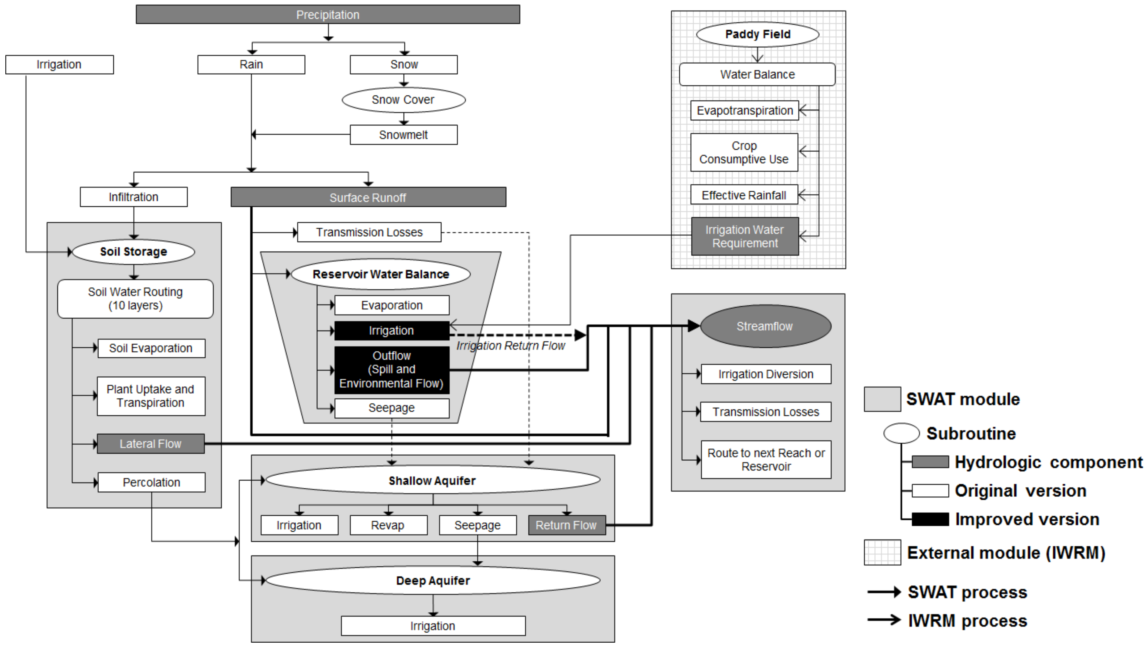
2.2. SWAT Modified Reservoir Operation Module

SWAT is continuous, long-term, distributed-parameter model designed to predict the effects of land management practices on hydrology, sediment, and contaminant transport in agricultural watersheds under varying soils, land use, and management conditions [25]. The SWAT model was adopted for the analysis of watershed hydrology, including agricultural reservoir operation. SWAT2009 version 488 with the ArcSWAT interface was used in this study. The water balance for reservoir, including inflow, outflow, surface rainfall, evaporation, seepage from the reservoir bottom, and diversions, is given by Equation (4):

$$V=V_{stored}+V_{flowin}-V_{flowout}+V_{pcp}-V_{evap}-V_{seep}$$

(4)

where V is the volume of water in the impoundment at the end of the day (m³), $V_{stored}$ is the volume of water stored in the water body at the beginning of the day (m³), $V_{flowin}$ is the volume of water entering the water body during the day (m³), $V_{pcp}$ is the volume of precipitation falling on the water body during the day (m³), $V_{evap}$ is the volume of water removed from the water body by evaporation during the day (m³), and $V_{seep}$ is the volume of water lost from the water body by seepage (m³).

In the case of an agricultural reservoir watershed, SWAT cannot evaluate the reservoir water supply to satisfy both IWR to downstream rice paddy areas via canal networks and EFR to downstream aquatic ecosystems by direct release from the reservoir. Moreover, the application of the original model to agricultural reservoir watersheds under existing irrigation practices is not possible because the excess irrigation flow is returned to the stream through the drainage canal system; that is, the irrigation return flow contributes to the streamflow at the outlet during the irrigation period. Therefore, the new option is added to the current reservoir simulation module of the SWAT to satisfy both the IWR and EFR within the typical reservoir water level operation rule. The SWAT can simulate the IWR and EFR with the reservoir inflow from the watershed by applying the new reservoir operation option in this study.

The outflow can be quantified using one of four different methods in the reservoir control module (IRESCO) of the original SWAT model [36]: measured daily outflow, measured monthly outflow, average annual release rate for an uncontrolled reservoir, and controlled outflow with target release. There is just one input option for lower and upper bound outflows in SWAT, even for multiple reservoirs in a watershed. Thus, the reservoir module was added to set different lower and upper bound outflows for each reservoir in a watershed, with different operation rules. The new reservoir simulation module (IRESCO = 4) contains four aspects: (1) simulation of auto-irrigation from SWAT coupled with IWR from IWRM, (2) application of Restriction Water Level (RWL) while supplying IWR and EFR, (3) inclusion of reservoir operation to determine the available release of EFR from the reservoir, and (4) consideration of return flow to streamflow. With the new module, the reservoir release is first filtered with the specified reference RWL, and the release amount of a day is shared for IWR and EFR. Figure 2 visualizes this concept.

When calculating the reservoir outflow from daily IWR and EFR (IRESCO = 4), the user must run the IWRM beforehand and provide the IWRM output as a file to reference the reservoir outflow daily. The volume of outflow from the reservoir during the irrigation period from the middle of April to the early period of September was then calculated:

$$V_{flowout}=V_{IWR} if waterlevel>DWL$$

(5)

where V_IWR is the daily IWR for the day during the irrigation period (m³), the water level is the calculated reservoir water level for the day (EL.m), and DWL is the dead water level (EL.m), which is the RWL for the irrigation water supply.

The volume of outflow from the reservoir during the non-irrigation period was then calculated:

$$V_{flowout}=q_{envflow}·\mathrm{86,400} if waterlevel>RW{L}_n$$

(6)

where q_envflow is the environmental flow for the day during the non-irrigation period (m³/s), RWL is the restricted water level (EL.m) for the environmental water supply (up to five layers can be set up by the user within the range from DWL to high water level (HWL)), and n is the RWL number from 1 to 5.

The user can specify the irrigation return flow. Irrigation return flow is the fraction of V_IWR, not the volume of water flowing out of the water body as V_flowout. Therefore, if the irrigation return flow fraction is specified, then the return flow for a given day is calculated as follows:

$$q_{IWRreturn}=\left(V_{IWR}·IW{R}_k\right)/\mathrm{86,400}$$

(7)

where $q_{IWRreturn}$ is the irrigation return flow for the day during the irrigation period (m³/s), and IWR is the fraction of V_IWR.

Table A2. List of added outgoing variables of the subroutine in the improved SWAT reservoir module (needed if IRESCO = 4).

Subroutine	Name	Unit	Definition
readres.f	RSVORD(:)	none	Number of water level measurement points
	RSVHWL(:)	EL.m	High water level
	RSVDWL(:)	EL.m	Dead water level
	RSVWL(:,:)	EL.m	Water level for each measurement point in relation curve between water level and storage capacity
	RSVST(:,:)	m3	Storage for each measurement point in relation curve between water level and storage (read in as 103 m3 and converted to m3)
	IRRTFF(:)	fraction	Irrigation return flow as a fraction of the irrigation water requirement volume (0–1)
	RSVRWL(:)	EL.m	Release restricted water level
	ENVFLOR(:)	m3	Environmental flow for each RWL (read in as m3/s and converted to m3)
res.f	RSVCWL(:)	EL.m	Calculated water level
	IWR	m3	Irrigation water requirement
	IRRTFO	m3/s	Irrigation return flow
	ENVFLOW	m3	Environmental flow

shows the list of additional variables for the two subroutines in the Fortran SWAT source files (readres.f and res.f); readres.f reads the data from the reservoir input file (*.res), and res.f routes water and sediment through reservoirs and computes evaporation and seepage from the reservoir. The improved SWAT model requires different input parameters (

Table A3. The input and output datasets of the improved SWAT reservoir module.

Data	Input (*.res)	Output (Output.rsv)
Reservoir characteristic	Relation curve between water level (EL.m) and storage capacity (103 m3) HWL and DWL (EL.m)	Water level on day (EL.m) Irrigation water requirement on day (m3) Irrigation return flow on day (m3/s) Environmental flow on day (m3)
Irrigation water	Beginning and ending dates of the irrigation period (mm/dd–mm/dd) Daily irrigation water requirement (103 m3) calculated by IWRM Irrigation return flow fraction (0~1)
Environmental flow	RWL (EL, m) (able to be set to five RWL) Environmental flow rate for each RWL

), including reservoir characteristics, irrigation water, and environmental flow.

First, the reservoir characteristics describe the relationship between the water level and storage capacity, which is used to interpolate the reservoir water level by calculated storage. Additionally, high (HWL) and dead (DWL) water levels are used to distinguish the water supply, if possible. For irrigation water supply, the user should define the beginning and end dates of the irrigation period. The remaining time is then defined as a non-irrigation period. The irrigation water supply from the reservoir and its return flow are calculated. Finally, to supply water for environmental flow, the user should determine the restricted water level (RWL) and its flow rate for each range (between DWL and HWL).

3. Evaluating the Model with the Anseong Watershed Dataset

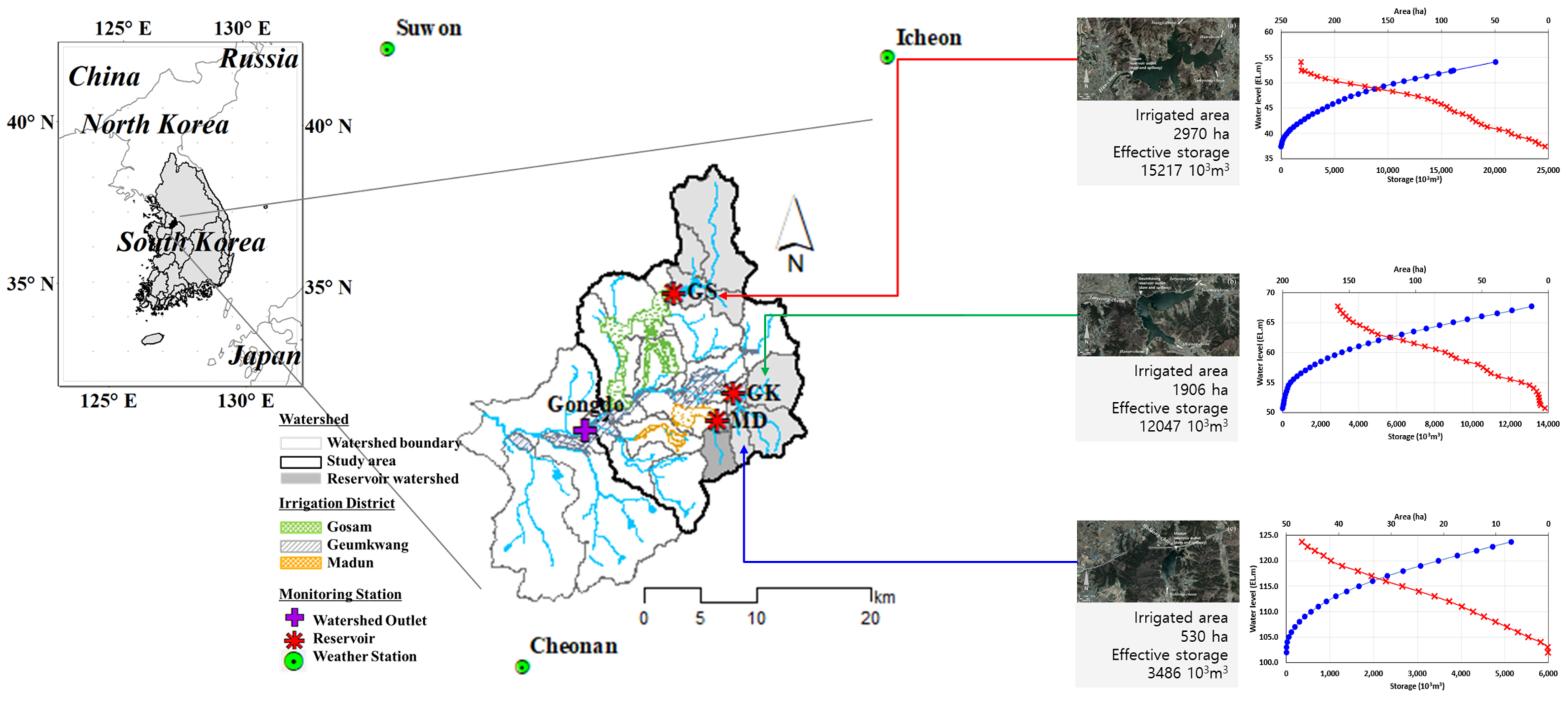
3.1. Study Watershed and Reservoirs

The Anseong watershed, in northwest South Korea within the latitude and longitude range of 127.1° to 127.3° E and 36.5° to 37.1° N, includes many agricultural reservoirs along the watershed’s main stream and tributaries. Figure 3 illustrates the watershed, which has a total area of 366.5 km². Agricultural reservoirs with less than 10 million m³ of storage capacity are the most widely distributed. Among the reservoirs, smaller reservoirs are managed by the local government, and the KRC manages the larger reservoirs. A total of 90 agricultural reservoirs in the watershed have a 41.9 million m³ storage capacity and provide irrigation water for 7264 ha in the benefiting area. The three largest reservoirs, Gosam (GS), Geumkwang (GK), and Madun (MD), located upstream of the watershed, have storage rates of 15.2, 12.0, and 3.5 million m³, respectively. These three reservoirs supply irrigation water for 50.9% (3696 ha) of the total benefiting area; the watershed outlet is Gongdo (GD) station, which has streamflow monitoring data. The characteristics of these reservoirs are shown in

Table 1. Specifications of three agricultural reservoirs.

Input Model	Parameter	Reservoir
		Gosam	Geumkwang	Madun
Area (ha)	Watershed area	7100	4830	1240
	Irrigated area	2970	1906	530
	Full water area	229.9	138.4	40.5
Storage (103 m3)	Gross storage	16,150	12,095	3496
	Effective storage	15,217	12,047	3486
	Dead storage	888	48	10
Water level (EL.m)	Full water level	54.1	67.7	120.8
	High water level	52.4	67.0	119.1
	Dead water level	40.8	51.5	102.0

.

3.2. Data Acquisition and Setup for Simulation

In order to estimate IWR, climatic, crop, soil, and irrigation data are required. Climatic data including daily precipitation (mm/day), minimum and maximum temperature (°C), mean wind speed (m/s), relative humidity (%), and sunshine hours (h) were collected by the Korea Meteorological Administration (KMA) at three weather stations (Suwon, Icheon, and Cheonan) over 21 years (1998–2018). Crop, soil, and irrigation data for each reservoir (GS, GK, and MD) were provided by KRC, and daily reservoir water level data for the same period as the climatic data were also collected. Data from the nearest meteorological station were included when simulating the irrigation water requirement for each reservoir.

Streamflow data required for SWAT calibration in GD was collected from Water Resources Management Information System (WAMIS). The 30 m DEM, land use, and soil map data from WAMIS for SWAT simulation were collected from Kim et al. [38].

4. Results and Discussion

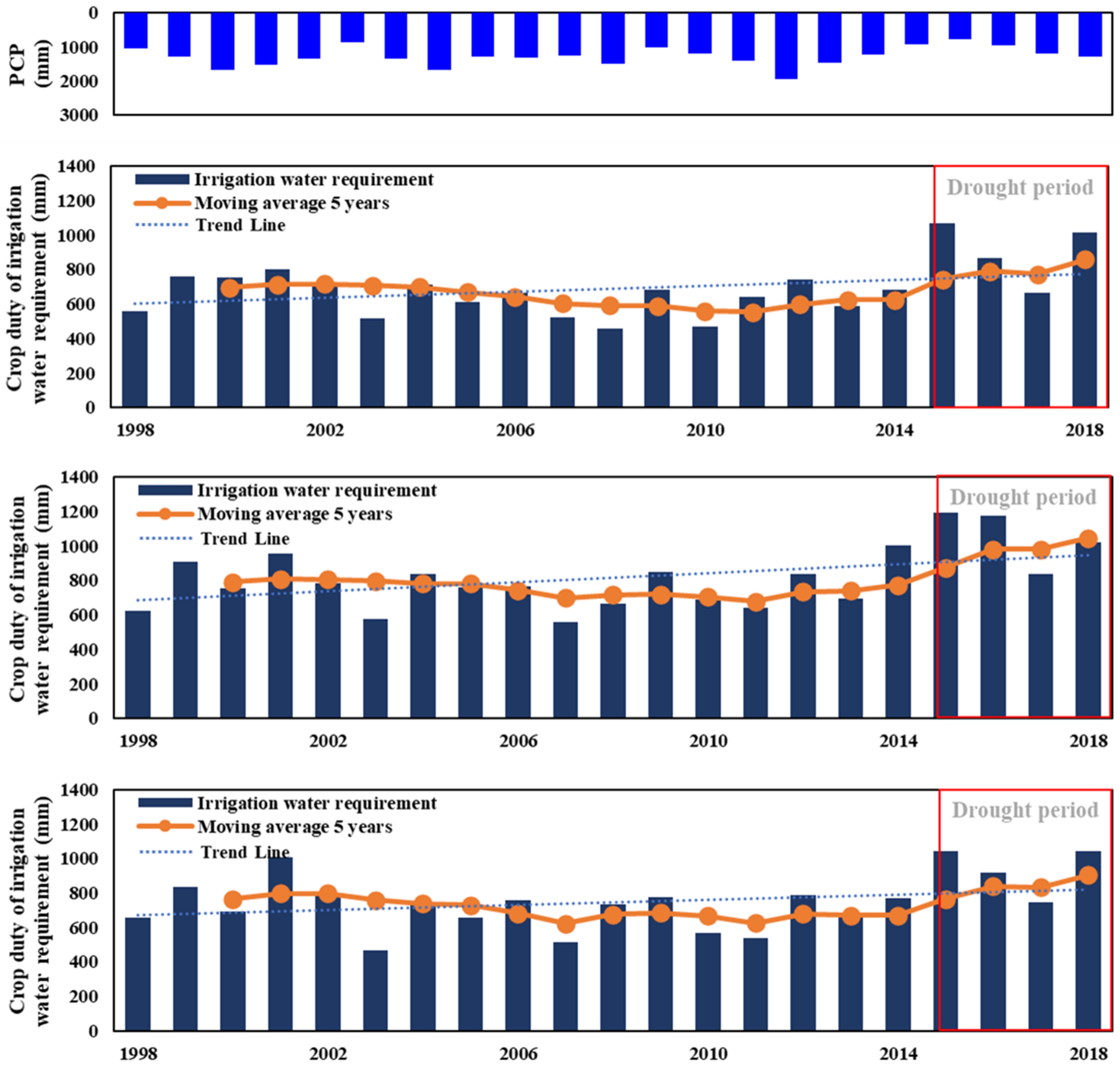
4.1. Irrigation Water Requirement of Reservoirs

The improved SWAT can input the IWR and EFR for each item when inputting reservoir release data. In the absence of observation data for IWR and EFR release, IWRM can be used to estimate the release according to the reservoir activity rules when inputting discharge data. To calculate the irrigation water requirement using the IWRM model, rice cultivation data such as irrigated area, irrigation schedule by phenological stages of paddy rice, ponding depth, and water conveyance loss are required.

Agricultural reservoirs are the critical source of water for the supply of irrigation water to paddy fields, and are mainly filled with precipitation during non-irrigation periods, which run from October to the end of March. Changes in meteorological and hydrological components such as precipitation, temperature, evapotranspiration, and watershed runoff will affect the demand for irrigation and agricultural water supply [39,40]. The effect of these non-irrigation treatments determines the water supply for irrigation.

The IWRM was calculated for 21 years (1998–2018) of daily IWS in three irrigated areas (GS, GK, MD). Figure 4 shows the annual GIWR calculated for the three irrigated areas, and

Table 2. The monthly mean IWRM results for the three irrigated areas during 1998–2018 (IWR: Irrigation water requirement, CUW: Consumptive use water, ET: Evapotranspiration, ER: Effective rainfall).

Unit: mm/month
IWRM Result	Apr	May	Jun	Jul	Aug	Sep	Total
Gosam reservoir
IWR	10.5	61.4	300.7	103.0	172.8	53.4	701.8
CUW	216.3	213.3	333.2	294.2	318.9	88.2	1464.1
- ET	50.6	137.4	142.1	124.0	130.7	36.5	621.2
- ER	32.4	98.1	70.1	204.0	167.7	41.4	613.7
Geumkwang reservoir
IWR	9.2	10.2	344.2	137.1	238.9	136.8	876.4
CUW	162.0	250.1	359.3	327.8	362.9	197.9	1659.9
- ET	15.6	142.1	145.6	128.2	126.1	64.0	621.6
- ER	14.7	86.6	84.0	218.1	171.7	88.5	663.4
Madun reservoir
IWR	7.8	6.4	255.4	95.9	160.7	97.3	623.5
CUW	156.0	197.3	319.0	278.3	317.3	169.3	1437.2
- ET	14.0	130.9	135.0	125.2	126.7	65.1	596.9
- ER	16.1	82.0	89.0	191.9	172.7	81.7	633.5

summarizes the monthly average IWR (m³/yr) for the three irrigated areas during 1998–2018. Among the three irrigated areas, the GIWR of the GK irrigated area is the largest, with an average value of 816.7 mm. On the other hand, the GIWR of the GS irrigated area is the lowest, with an average value of 691.6 mm. The average GIWR of the three irrigated areas was 754.1 mm, with an annual average precipitation of 1278.3 mm during 1998–2018. The calculated annual average IWR was calculated by multiplying the irrigated area (ha) and the GIWR (mm/yr) for the GS, GK, and MD irrigated areas, which were 20.5, 15.6, and 4.0 million m³/yr, respectively. The total annual amount of IWR in the study area was 40.1 million m³, which was the water requirement of the reservoirs in the area. The calculated daily IWR for each irrigated area was specified in the SWAT and improved SWAT as measured daily outflow data.

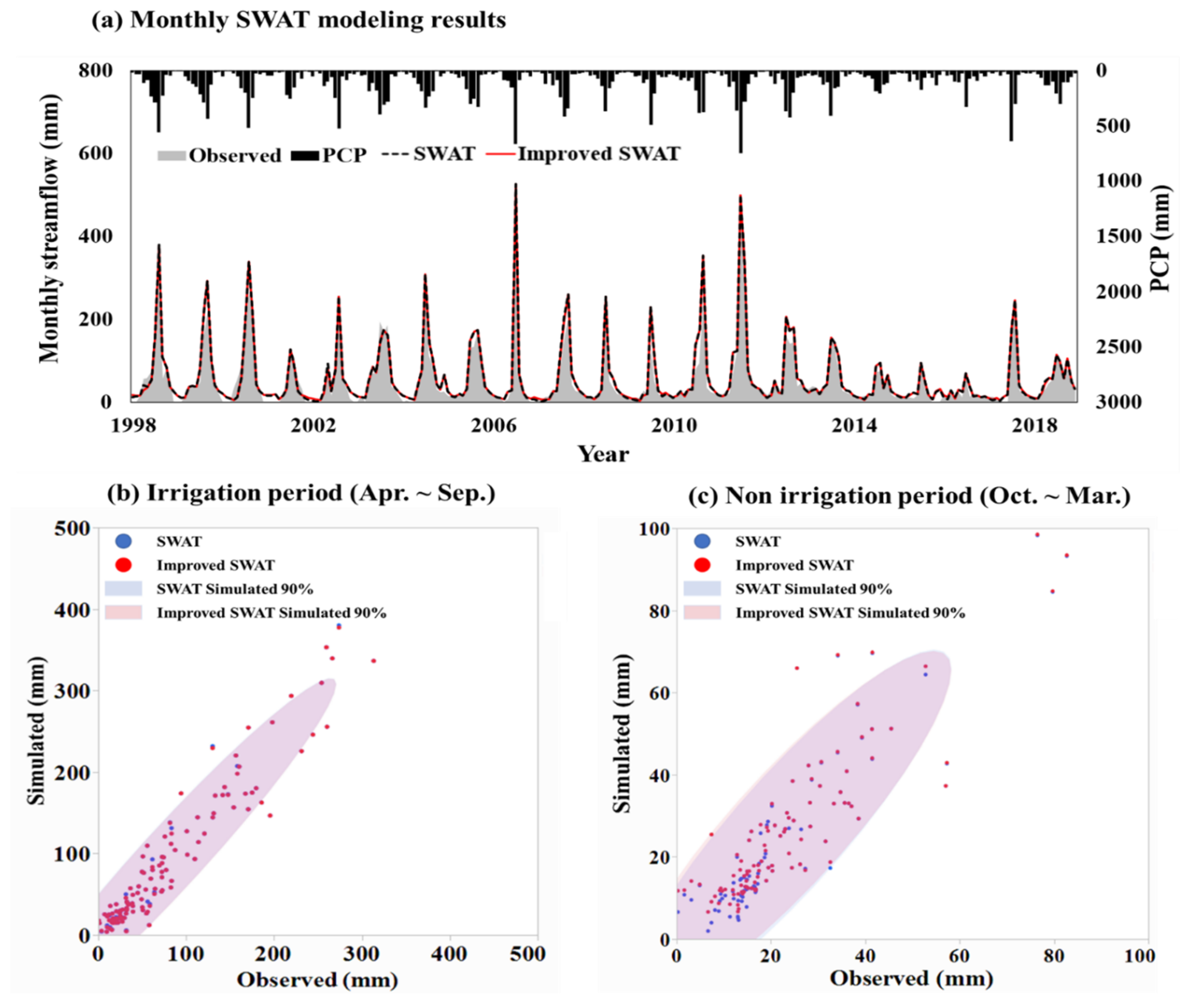
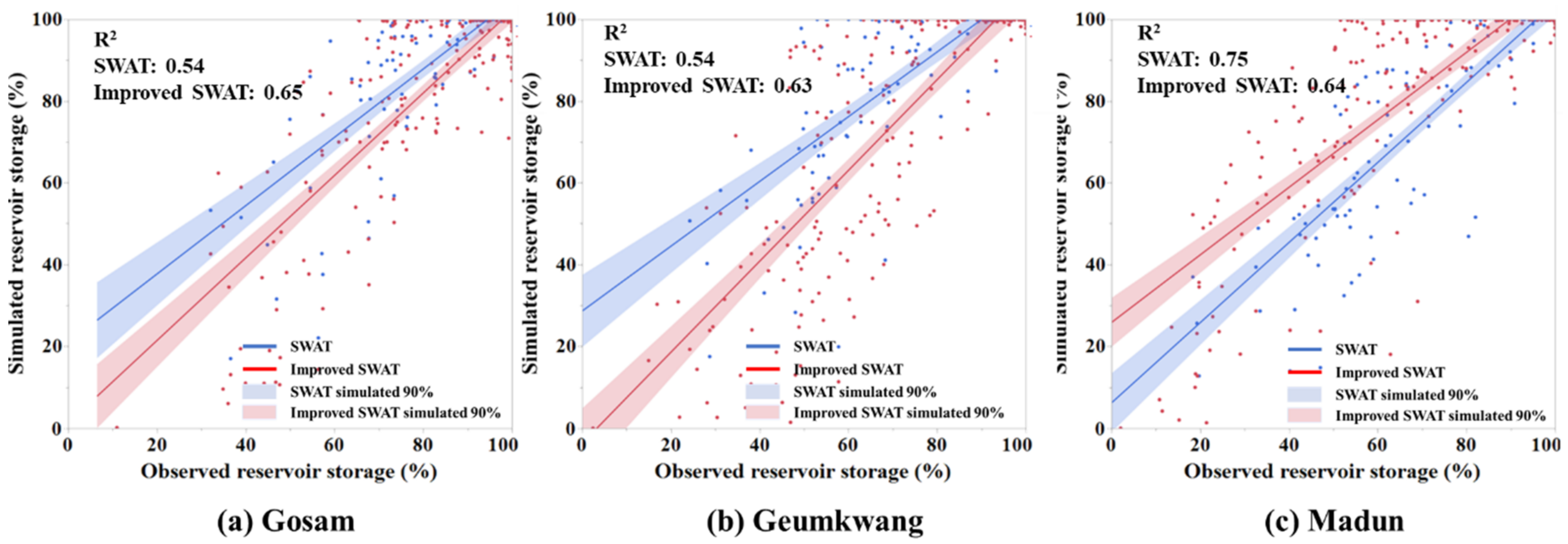
4.2. Improved SWAT Calibration and Validation Results

To compare the SWAT model and the Improved SWAT before environmental flow was applied, calibration was performed on the GD station with the same parameters and for the same period. The SWAT and improved SWAT models were set up for two years (1996–1997) and calibrated for seven years (1998–2005), and validated for 13 years (2006–2018) with daily streamflow data at GD station.

The model performance was quantitatively assessed by calculating the coefficient of determination (R²), Root-mean-square error (RMSE), and Nash-Sutcliffe model efficiency (NSE). R² ranges from 0 to 1, NSE ranges from −1 to 1, and that both coefficients are close to 1 indicates a perfect simulation with no divergence from observed data [41]. The standard deviation of the residual is represented as the error between the observed and simulated values by RMSE, an extensively used error index statistic [42].

Parameter estimation followed the determination of the simulation model parameters to be calibrated. Manual calibration and autocalibration are two approaches to parameter estimation [43]. Manual calibration is the most widely used approach for complex models, including the distributed type [44,45,46]. The improved SWAT was calibrated using a manual calibration process. A total of twelve parameters in four categories were selected for calibration: runoff (CH_N1 and CH_N2), evapotranspiration (ESCO), groundwater (GW_DELAY, ALPHA_BF, and GW_REVAP), snowmelt (SFTMP, SMTMP, and SNO50COV), and reservoir (RES_K, EVRSV, and IRRTFF). For the three reservoirs (GS, GK, and MD), calibration was performed including the reservoir parameters, and the watershed outlet in GD was calibrated for three categories and nine parameters, excluding the reservoir parameters. The initial and adjusted values of the calibrated parameters are listed in

Table A4. Calibrated IWRM and improved SWAT model parameters at three reservoirs and outlet points.

Parameter	Initial Value	Adjusted Value
		GS	GK	MD	GD (Outlet)
Runoff and evapotranspiration
ESCO	0.95	0.8	0.8	0.8	0.8
CH_N1/CH_N2	0.014	0.033	0.033	0.033	0.033/0.025
Groundwater
GW_DELAY (days)	31	80	80	80	55.75
ALPHA_BF (days)	0.048	0.5	0.6	0.5	0.37
GW_REVAP	0.02	0.2	0.2	0.2	0.2
Snowmelt
SFTMP (°C)	1	−1.3	−1.3	−1.3	−1.3
SMTMP (°C)	0.5	4.2	4.2	4.2	4.2
SNO50COV	0	0.47	0.47	0.47	0.47
Reservoir
RES_K (mm/hr)	0	0.2	0.3	0.3	-
EVRSV	0.6	0.5	0.6	0.6	-
IRRTFF	0	0.35	0.35	0.35	-

.

Table 3. Statistical summary of the improved SWAT results (Irrigation: ~Apr.–Sep., Non-irrigation: ~Oct.–Mar., Obs.: Observed, and Impv.S: Improved SWAT).

Periods	PCP (mm)	Streamflow (mm)			Evaluation Criteria
		Obs.	SWAT	Impv.S	R2		RMSE (mm/day)		NSE
					SWAT	Impv.S	SWAT	Impv.S	SWAT	Impv.S
Irrigation	1086.0	497.7	571.2	566.7	0.93	0.93	30.6	30.3	0.88	0.89
Non-irrigation	203.8	115.3	143.0	148.6	0.80	0.79	8.8	8.8	0.93	0.93
Total	1289.8	613.0	714.1	718.9	0.87	0.86	19.70	19.54	0.91	0.91

shows the statistical summary of the model calibration and validation, and Figure 5 shows comparisons of the observed and improved SWAT simulated streamflow. For the performance comparison of the two models, parametric calibration was performed based on the existing SWAT. The observed and simulated daily streamflow at the two locations matched reasonably well. The improved SWAT gave streamflow results for average R², RMSE, and NSE of 0.86, 19.54 mm/day, and 0.91, respectively, whereas SWAT gave 0.87, 19.70 mm, and 0.91, respectively.

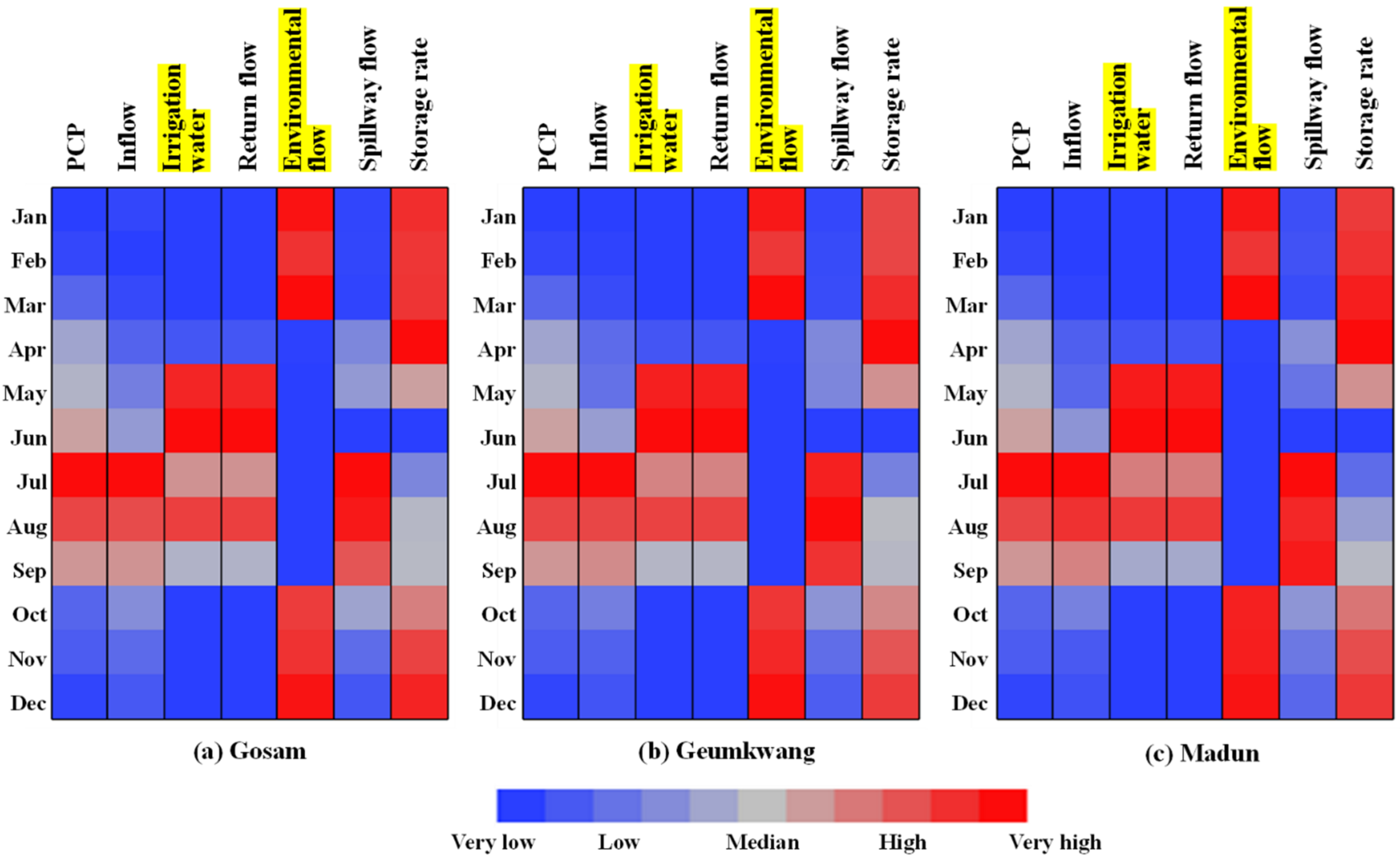
4.3. Improved SWAT Reservoir Operation

The improved SWAT can set the EFR based on the RWL. As conditions for releasing EFR in the non-irrigation season (October to April) in the Improved SWAT, RWL-1, RWL-2, and RWL-3 were set at 90%, 80%, and 70% of the effective reservoir storage, and the EFR amount was calculated according to each RWL by manual calibration. Figure 6 compares the observed and simulated SWAT and improved SWAT daily reservoir storage rate using only IWR at GS, GK, and MD reservoirs from 1998 to 2018 in the calibration and validation periods. Compared with SWAT, the R² of the improved SWAT significantly increased from 0.54, 0.54 to 0.65, 0.63, respectively, in the GS and GK reservoirs. However, the R² of the MD reservoir simulation results decreased by 0.75 to 0.64. This is because the MD Reservoir is smaller than the other two, and the actual release observations show that it provides less environmental water. As a result, the R² of the improvement SWAT with the EFR operation rules decreased. Nevertheless, the results demonstrate that the improved SWAT coupled with the IWRM modeling approach is reasonable to represent reservoir dynamics in the agricultural watershed.

Improved SWAT was proposed for multidisciplinary functions and the subsequent quantitative analysis of agricultural water. Figure 7 shows the basic reservoir rate derived from this study for the monthly reservoir activity law, with blue being relatively small and red being relatively high. Regarding the seasonal characteristics of Korea and the subsequent activity patterns of agricultural reservoirs, precipitation is concentrated in July and August, and irrigation water is commonly used in May and June. Environmental water in agricultural reservoirs has adequate storage capacity and the focus is on releasing it in winter rather than during the irrigation season. Improved SWAT provides a flexible water management schedule for paddy fields and systemizes the environmental use of agricultural water.

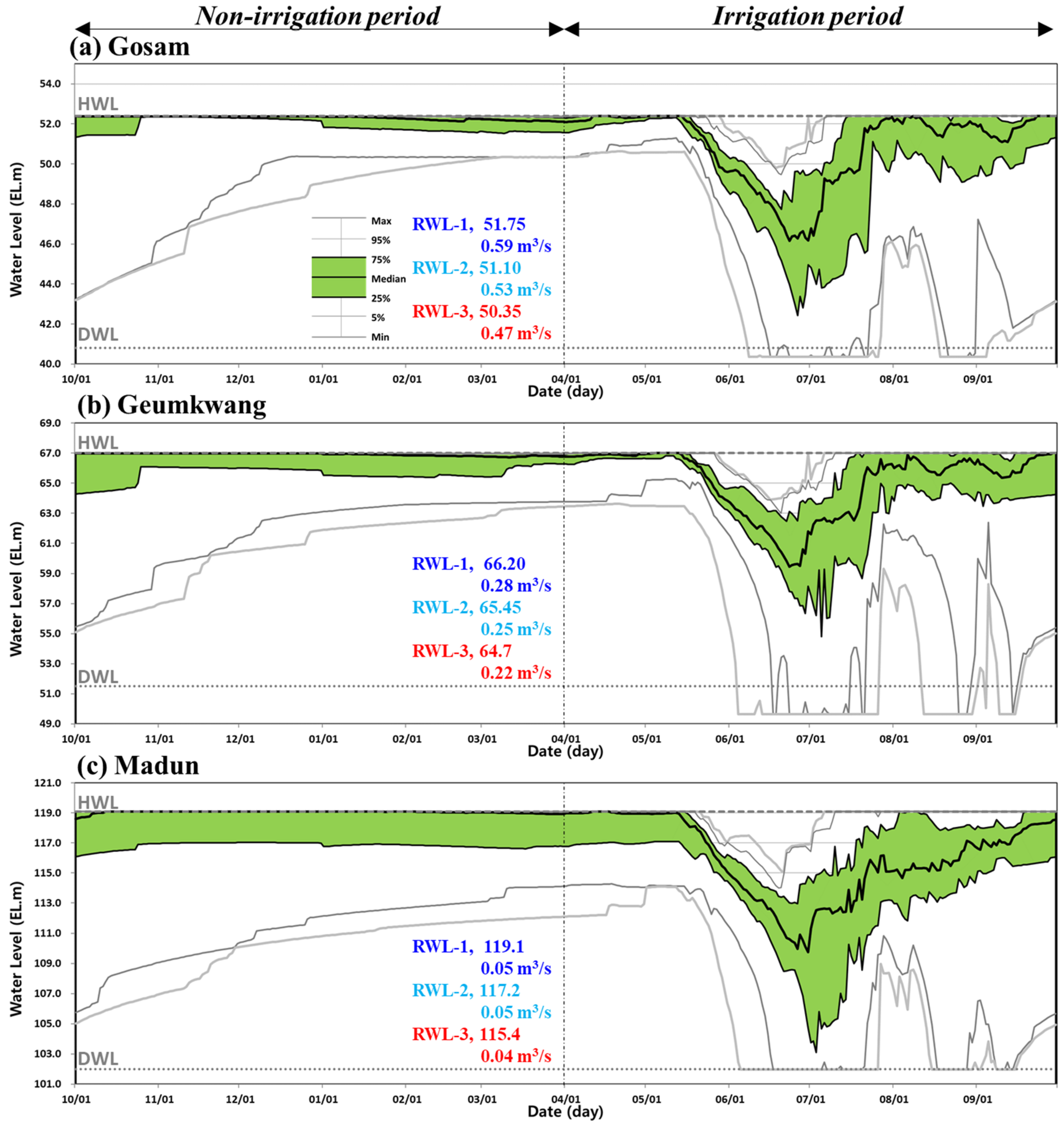
4.4. Streamflow Impact by Irrigation Water Supply and Environmental Flow Release

The improved SWAT reduced the R² efficiency compared to SWAT, but the RMSE and NSE were improved. This is because the resulting value of the improved SWAT is underestimated compared to SWAT, as shown in

Table 4. Alteration of the flow duration and coefficient of flow regime for selected years (CFR: coefficient of flow regime, Impv. S: improved SWAT, and Diff: difference between SWAT and improved SWAT).

Flow Duration		Streamflow (m3/s)					CFR
		Q10	Q95	Q185	Q275	Q355
Normal year	SWAT	52.35	5.71	3.35	1.85	0.94	55.69
	Impv.S	52.10	5.70	3.38	1.98	1.05	49.76
	Diff (%)	−0.49	−0.30	0.97	7.20	11.37	−10.65
Selected drought year (2001)	SWAT	16.27	3.16	2.17	1.45	0.66	24.75
	Impv.S	16.27	3.10	2.29	1.87	0.77	21.16
	Diff (%)	0.00	−1.93	5.49	29.19	16.96	−14.50
Selected flood year (2011)	SWAT	114.50	9.32	4.47	2.36	1.54	74.40
	Impv.S	114.50	9.28	4.45	2.36	1.57	73.07
	Diff (%)	0.00	−0.37	−0.43	0.08	1.82	−1.79

. Errors in low-flow predictions are attributed to uncertainties in quantifying the storage function of forest soils and in estimating the soil and groundwater parameters. Additionally, the efficiency of the non-irrigation period was different because environmental water could be considered during this period. However, it has been found that the efficiency of the irrigation period model is better than that of SWAT. This is because the pattern of the reservoir storage rate changed due to the release of ENF according to the restricted water level from October to April. In general, the model fits both the observed rise in streamflow and the recession reasonably well.

In Table 4, the flow duration at GD, such as flood flow (Q10), high flow (Q95), normal flow (Q185), low flow (Q275), and drought flow (Q355), were analyzed by comparison between SWAT and improved SWAT. The coefficient of flow regime (CFR) in the table is a flow duration coefficient, and the variability of the flow rate was compared by dividing flood flow by drought flow. In terms of precipitation, the years of flood and drought were selected as the year with the highest precipitation (1939.03 mm) and the year with the lowest precipitation (871.06 mm), respectively.

By considering the reservoir operating rule, Q10 and the normal year increased by −0.49% from 52.35 m³/s to 52.10 m³/s, and Q355 increased from 0.94 m³/s to 1.05 m³/s. Accordingly, the CFR decreased by −10.65% from 55.69 to 49.76. In the drought year, increased by 16.96% from 0.66 m³/s to 0.77 m³/s, and CFR also decreased −14.50%. Accordingly, it was found that the fluctuation of the flow was reduced through the reservoir operating rule according to the supply of EFR. On the other hand, in the normal year and the drought year, the difference reversed before Q185, whereas in the flood year, the difference was reversed after Q185. This result shows that the streamflow difference between flood year and drought year decreased from 0.88 m³/s to 0.80 m³/s, as the streamflow increased according to EFR supply even in drought year.

Although optimal water supply for EFR in each agricultural reservoir was calculated by trial and error, a genetic algorithm was used for the optimal operating policy, as in Anand et al. [47]; alternatively, the optimal reservoir operation rule can be developed by developing a module that can calculate hydroelectric power according to reservoir operation.

The operating rule curve was shown to divide periods of irrigation (1 April to 30 September) and non-irrigation (1 October to 31 March). Using the operating rule curve, the user may want to maintain flexible reservoir operations depending on weather conditions. The operating rule curve was presented as the percentile rank of the daily reservoir water level, based on the results of reservoir operation using weather data over 21 years (1998–2018). The water levels for each percentile were divided into three buffer sections representing drought (5~25%), normal (25~75%), and flood (75~95%) years to operate the agricultural reservoir with the operating rule curve [48]. Figure 8 shows the optimized operating rule curve for the GS, GK, and MD reservoirs.

Through the operating rule curve according to the operating rule for multiple water supply, it is possible to know the discharge amount for each RWL and the range of the minimum and maximum reservoir storage levels per day. The reason why the reservoir storage level in the irrigation period is greater than that in the non-irrigation period is that the spring drought occurs in ~April–May, and the use of irrigation water increases from June onwards after the ponding period begins. According to the presence or absence of rainfall, the change in reservoir storage levels during July was the largest.

Many challenges have been met by efforts to incorporate environmental flows. A system of prioritization among water uses involves many water allocation systems that either do not favor environmental flow conservation, or do not allow for ecological protection from high flow events [49]. Major progress in environmental flow management has been made in recent years because of various factors, including government dedication to environmental flow projects, increases in scientific expertise, and processes for evaluation which involve greater stakeholder collaboration and co-design. However, shared water resources also create tension between stakeholders because of different goals and objectives [50].

Attempts to measure agricultural losses related to habitat conservation have mainly focused on evaluating the effects of water distribution plans (in the sense of alternative agricultural and environmental policy scenarios) or on examining variations in crop yield losses [51,52]. In addition, EFR was calculated by introducing analysis and modeling methods such as the Hydroecological Integrity Assessment Process (HIP) and Ecological Limits of hydrologic alteration (ELOHA) [53,54]. However, the contradictory nature of water use means that one goal cannot be changed without degrading one or more other goals, especially in arid and semi-arid areas. These inconsistencies tend to be irreconcilable contradictions in semi-arid areas. Little attention has been paid to reducing the economic losses incurred by the maintenance of environmental flows by considering the seasonality of hydrological conditions and water requirements. Exploring these variables will enable us to obtain the best environmental flow management [55].

Improved SWAT, as a modification of the SWAT reservoir operation module, can also be used in other areas as it can automatically satisfy IWR and EFR at the same time by inputting the RLW and the corresponding discharge amount for each reservoir. In the future, it will be possible to evaluate EFR according to climate change scenarios and land use changes through the development of a module that automatically finds the amount of discharge that meets the RWL.

5. Conclusions

In this study, we attempted to assess the potential impact of agricultural water management in terms of reservoir operation and watershed hydrologic processes. The methods presented here were the developed IWRM and the improved SWAT model, based on a new operating rule curve for a multiple water supply (IWR and EFR).

IWRM calculates the amount of irrigation water requirement in an agricultural area, which is calculated as the discharge of the SWAT Reservoir. It was confirmed that the calibration results of SWAT and Improved SWAT applied only with IWR were R2 0.01, RMSE 0.16 mm/day, and NSE 0.00, showing no significant difference. In the Improved SWAT with IWR, the limiting level according to the low yield was set and the EFR for each limiting level was applied. R² increased from 0.54 and 0.54 to 0.65 and 0.63 in the GS and GK reservoirs, respectively, though not in the MD reservoirs with small watersheds, and improved SWAT confirmed the reservoir dynamics.

The flow regime was calculated to evaluate the effect of the reservoir’s river maintenance flow at GD station, a watershed outlet, and it was confirmed that Q355, a drought flow, increased by 11.37% in the normal year and 16.96% in the drought year. The improved SWAT reservoir simulation module for multiple water supply-related EFR in agricultural reservoirs was examined, including one of the most critical operating rule curves. This present study focuses on evaluating methods to provide adequate information to water managers and others.

Future research based on this study may include assessment of the water quality improvement of multiple water supplies in reservoirs, designing water requirements for paddy rice affected by climate change, and optimizing operation rule curves for agricultural reservoirs for environmental flow, flood (or drought) control, and aquatic activities under changed hydrological regimes. The literature includes individual details of climate change impacts and of adaptations for agricultural water management. Thus, there is a need to explore the use of various environmental change scenarios to produce better information. When combined with the framework in this study and further research, Improved SWAT will provide useful information for local decision makers and water managers in understanding and evaluating future climate change impacts on agricultural water resources, the environment, and water quality management in agricultural watersheds.

References

1. Nilsson, C.; Reidy, C.A.; Dynesius, M.; Revenga, C. Fragmentation and flow regulation of the world’s large river systems. J. Sci. 2005, 308, 405–408. [Google Scholar] [CrossRef] [Green Version]
2. Lee, J.W.; Lee, Y.G.; Woo, S.Y.; Kim, W.J.; Kim, S.J. Evaluation of water quality interaction by dam and weir operation using SWAT in the Nakdong River Basin of South Korea. Sustainability 2020, 12, 6845. [Google Scholar] [CrossRef]
3. Acreman, M.; Aldrick, J.; Binnie, C.; Black, A.; Cowx, I.; Dawson, H.; Dunbar, M.; Extence, C.; Hannaford, J.; Harby, A.; et al. Environmental flows from dams: The water framework directive. In Proceedings of the Institution of Civil Engineers-Engineering Sustainability; Thomas Telford, Ltd.: London, UK, 2009; pp. 13–22. [Google Scholar]
4. Acreman, M.; Angela, H.A.; Matthew, J.C.; Carol, C.; Neville, D.C.; Fiona, D.; Ian, O.; Carmel, A.P.; Michael, J.S.; William, Y. Environmental flows for natural, hybrid, and novel riverine ecosystems in a changing world. Front. Ecol. Environ. 2014, 12, 466–473. [Google Scholar] [CrossRef] [Green Version]
5. Alfredsen, K.; Harby, A.; Linnansaari, T.; Ugedal, O. Development of an inflow-controlled environmental flow regime for a Norwegian river. River Res. Appl. 2012, 28, 731–739. [Google Scholar] [CrossRef] [Green Version]
6. Haghighi, A.T.; Kløve, B. Design of environmental flow regimes to maintain lakes and wetlands in regions with high seasonal irrigation demand. Ecol. Eng. 2017, 100, 120–129. [Google Scholar] [CrossRef] [Green Version]
7. King, A.J.; Tonkin, Z.; Mahoney, J. Environmental flow enhances native fish spawning and recruitment in the Murray River, Australia. River Res. Appl. 2009, 25, 1205–1218. [Google Scholar] [CrossRef]
8. Lytle, D.A.; Poff, N.L. Adaptation to natural flow regimes. Trends Ecol. Evol. 2004, 19, 94–100. [Google Scholar] [CrossRef]
9. Poff, N.L.; Allan, D.; Bain, M.B.; Karr, J.R.; Prestegaard, K.L.; Richter, B.D.; Sparks, R.E.; Stromberg, J.C. The natural flow regime. BioScience 1997, 47, 769–784. [Google Scholar] [CrossRef]
10. Tharme, R.E. A global perspective on environmental flow assessment: Emerging trends in the development and application of environmental flow methodologies for rivers. River Res. Appl. 2003, 19, 397–441. [Google Scholar] [CrossRef]
11. Liu, J.; Liu, Q.; Yang, H. Assessing water scarcity by simultaneously considering environmental flow requirements, water quantity, and water quality. Ecol. Indic. 2016, 60, 434–441. [Google Scholar] [CrossRef] [Green Version]
12. MLTM. Water Vision 2020; Ministry of Land, Transportation and Maritime Affairs: Sejong, Korea, 2016. (In Korean)
13. Kim, S.M.; Park, Y.K.; Won, C.H.; Kim, M.H. Analysis of scenarios for environmental instream flow considering water quality in Saemangeum Watershed. J. Korean Soc. Eng. 2016, 38, 117–127. (In Korean) [Google Scholar] [CrossRef]
14. MFAFF. Statistical Yearbook of Land and Water Development for Agriculture; Ministry for Food, Agriculture, Forestry and Fisheries: Gwacheon, Korea, 2009. (In Korean)
15. KRC. The Project of Raising Embankment of Agricultural Reservoir; Korea Rural Community Corporation: Naju-si, Korea, 2011. (In Korean) [Google Scholar]
16. Park, J.Y.; Park, M.J.; Joh, H.K.; Shin, H.J.; Kwon, H.J.; Srinivasan, R.; Kim, S.J. Assessment of MIROC3.2 HiRes climate and CLUE-s land use change impacts on watershed hydrology using SWAT. Trans. ASABE 2011, 54, 1713–1724. [Google Scholar] [CrossRef]
17. Kim, S.J.; Kim, P.S.; Lim, C.Y. Behaviour analysis of irrigation reservoir using open water management program. J. Korean Soc. Agric. Eng. 2004, 46, 3–13. (In Korean) [Google Scholar]
18. Kim, S.J.; Park, K.C.; Park, H.S. Estimation of available permit water for large scale agricultural reservoirs in Youngsan River basin. J. Korean Soc. Agric. Eng. 2012, 54, 93–97. (In Korean) [Google Scholar]
19. Kim, P.S.; Kim, S.J. Development of storage management system for small dams. J. Korean Soc. Agric. Eng. 2005, 47, 15–25. (In Korean) [Google Scholar]
20. Lee, N.H.; Heo, Y.J. Reliability and applicability of weather forecasts for irrigation scheduling. J. Korean Soc. Agric. Engin. 1999, 41, 25–32. (In Korean) [Google Scholar]
21. Hatterman, F.; Krysanova, V.; Wechsung, F.; Wattenbach, M. Integrating groundwater dynamics in regional hydrological modelling. Environ. Model. Softw. 2004, 19, 1039–1051. [Google Scholar] [CrossRef]
22. Kannan, N.; Jeong, J.; Srinivasan, R. Hydrologic modeling of a canal-irrigated agricultural watershed with irrigation best management practices: Case study. J. Hydrol. Eng. 2011, 16, 746–757. [Google Scholar] [CrossRef] [Green Version]
23. Cau, P.; Paniconi, C. Assessment of alternative land management practices using hydrological simulation and a decision support tool: Arborea agricultural region, Sardinia. Hydrol. Earth Syst. Sci. 2007, 11, 1811–1823. [Google Scholar] [CrossRef] [Green Version]
24. Piniewski, M.; Cedric, L.R.; Acreman, M.C.; Okruszko, T.; Schneider, C. Effect of climate change on environmental flow indicators in the Narew Basin, Poland. J. Environ. Qual. 2014, 43, 155–167. [Google Scholar] [CrossRef] [PubMed] [Green Version]
25. Arnold, J.G.; Srinivasan, R.; Muttiah, R.S.; Williams, J.R. Large-area hydrologic modeling and assessment: Part I. Model development. J. Am. Water Resour. Assoc. 1998, 34, 73–89. [Google Scholar] [CrossRef]
26. Cai, X.; McKinney, D.C.; Lasdon, L.S. A framework for sustainability analysis in water resources management and application to the Syr Darya Basin. Water Resour. Res. 2002, 38, 1–14. [Google Scholar] [CrossRef]
27. Chang, L.C. Guiding rational reservoir flood operation using penalty-type genetic algorithm. J. Hydrol. 2008, 354, 65–74. [Google Scholar] [CrossRef]
28. Allen, R.G.; Pereira, L.S.; Raes, D.; Smith, M. Crop Evapotranspiration. Guidelines for Computing Crop Water Requirements; FAO Irrigation and Drainage Paper 56; FAO: Rome, Italy, 1998. [Google Scholar]
29. Chung, H.W.; Kim, S.J.; Kim, J.S.; Noh, J.K.; Park, K.U.; Son, J.K.; Yoon, K.S.; Lee, K.H.; Lee, N.H.; Chung, S.O.; et al. Irrigation and Drainage Engineering, 2nd ed.; Dongmyeong Publisher: Seoul, Korea, 2006. (In Korean) [Google Scholar]
30. Yoo, S.H.; Choi, J.Y.; Jang, M.W. Estimation of design water requirement using FAO Penman-Monteith and optimal probability distribution function in South Korea. Agric. Water Manag. 2008, 95, 845–853. [Google Scholar] [CrossRef]
31. Dastane, N.G. Effective Rainfall in Irrigated Agriculture; FAO Irrigation and Drainage. Paper, No. 25; Food and Agriculture Organization of the United Nations: Rome, Italy, 1978. [Google Scholar]
32. Jang, M.W.; Chung, H.W.; Choi, J.Y.; Park, K.W.; Bae, S.J. Development of a single reservoir agricultural drought evaluation model for paddy. J. Korean Soc. Agric. Eng. 2004, 46, 17–30. [Google Scholar]
33. KRC. A Study on Causative Factors of Drying Streams in Rural Area; Korea Rural Community Corporation: Naju-si, Korea, 2006. (In Korean) [Google Scholar]
34. Yoo, S.H.; Choi, J.Y.; Nam, W.H.; Hong, E.M. Analysis of design water requirement of paddy rice using frequency analysis affected by climate change in South Korea. Agric. Water Manag. 2012, 112, 33–42. [Google Scholar] [CrossRef]
35. Jensen, M.E.; Burman, R.D.; Allen, R.G. Evapotranspiration and Irrigation Water Requirements; ASCE Manual, No. 70; ASCE: New York, NY, USA, 1990. [Google Scholar]
36. Neitsch, S.L.; Arnold, J.G.; Kiniry, J.R.; Williams, J.R.; King, K.W. Soil and Water Assessment Tool: Theoretical Documentation; Version 2000. TWRI Report TR-191; Texas Water Resources Institute: College Station, TX, USA, 2002. [Google Scholar]
37. Park, J.Y. Improvement of SWAT Model for Agricultural Water Management Adapting Climate Change. Ph.D. Thesis, Konkuk University, Seoul, Korea, 2013. [Google Scholar]
38. Kim, D.R.; Lee, Y.G.; Lee, J.W.; Kim, S.J. Assessment of future climate and land use changes impact on hydrologic behavior in Anseong-cheon Gongdo urban-growing watershed. J. Korea Water Resour. Assoc. 2018, 51, 141–150. (In Korean) [Google Scholar]
39. Ashoften, P.S.; Haddad, O.B.; Mariño, M. Climate change impact on reservoir performance indexes in agricultural water supply. J. Irrig. Drain. Eng. 2013, 139, 85–97. [Google Scholar] [CrossRef]
40. Wu, Y.; Chen, J. Estimating irrigation water demand using an improved method and optimizing reservoir operation for water supply and hydropower generation: A case study of the Xinfengjiang Reservoir in southern China. Agricul. Water Manag. 2013, 116, 110–121. [Google Scholar] [CrossRef]
41. Nash, J.E.; Sutcliffe, J.V. River flow forecasting through conceptual models part I—A discussion of principles. J. Hydrol. 1970, 10, 282–290. [Google Scholar] [CrossRef]
42. Singh, J.; Knapp, H.V.; Arnold, J.G.; Demissie, M. Hydrological modeling of the Iroquois river watershed using HSPF and SWAT 1. JAWRA J. Am. Water Resour. Assoc. 2005, 41, 343–360. [Google Scholar] [CrossRef]
43. Muleta, M.K.; Nicklow, J.W. Sensitivity and uncertainty analysis coupled with automatic calibration for a distributed watershed model. J. Hydrol. 2005, 306, 127–145. [Google Scholar] [CrossRef] [Green Version]
44. Refsgaard, J.C. Parameterization, calibration and validation of distributes hydrologic models. J. Hydrol. 1997, 198, 69–97. [Google Scholar] [CrossRef]
45. Refsgaard, J.C.; Knudsen, J. Operational validation and intercomparison of different types of hydrologic models. Water Resour. Res. 1996, 32, 2189–2202. [Google Scholar] [CrossRef]
46. Senarath, S.U.S.; Ogden, F.L.; Downer, C.W.; Sharif, H.O. On the calibration and verification of two-dimensional, distributed, hortonian, continuous watershed models. Water Resour. Res. 2000, 36, 1495–1510. [Google Scholar] [CrossRef]
47. Kang, S.K.; Lee, D.R.; Moon, J.W.; Choi, S.J. Effects of dams and water use on flow regime alteration of the Geum River Basin. J. Korea Water Res. Assoc. 2010, 43, 325–336. (In Korean) [Google Scholar] [CrossRef] [Green Version]
48. Anand, J.; Gosain, A.K.; Kohsa, R. Optimisation of multipurpose reservoir operation by coupling soil and water assessment tool (SWAT) and algorithm for optimal operating policy (case study: Ganga River Basin). Sustainability 2018, 10, 1660. [Google Scholar] [CrossRef] [Green Version]
49. Richter, B.D. Re-thinking environmental flows: From allocations and reserves to sustainability boundaries. River Res. Appl. 2010, 26, 1052–1063. [Google Scholar] [CrossRef]
50. Farhadian, M.; Bozorg-Haddad, O.; Loáiciga, H.A. Fulfillment of river environmental flow: Applying Nash theory for quantitative-qualitative conflict resolution in reservoir operation. Water Environ. J. 2020, 35, 486–499. [Google Scholar] [CrossRef]
51. Farooq, N.; Gheewala, S.H. A review of two different methods for the estimation of water footprint of crops. Bull. Geol. Soc. Malays. 2019, 68, 85–90. [Google Scholar] [CrossRef] [Green Version]
52. Li, J.; Deng, W.; Zhang, J.F. Evaluating Mountain water scarcity on the county scale: A case study of Dongchuan District, Kunming, China. J. Mt. Sci. 2019, 16, 744–754. [Google Scholar] [CrossRef]
53. Pastor, A.V.; Ludwig, F.; Biemans, H.; Hoff, H.; Kabat, P. Accounting for environmental flow requirements in global water assessments. Hydrol. Earth Syst. Sci. 2014, 18, 5041–5059. [Google Scholar] [CrossRef] [Green Version]
54. Zeiger, S.J.; Hubbart, J.A. Assessing Environmental Flow Targets Using Pre-Settlement Land Cover: A SWAT Modeling Application. Water 2018, 10, 791. [Google Scholar] [CrossRef] [Green Version]
55. Pang, A.; Li, C.; Sun, T.; Yang, W.; Yang, Z. Trade-off analysis to determine environmental flows in a highly regulated watershed. Sci. Rep. 2018, 8, 14130. [Google Scholar] [CrossRef] [Green Version]
Figure 1. Flow chart of this study.
Water 13 02543 g001
Figure 2. The description of the model process by which the results of irrigation water supply are driven in SWAT [37].
Water 13 02543 g002
Figure 3. Map of Anseong watershed showing the sub-basins and the locations of the agricultural reservoirs.
Water 13 02543 g003
Figure 4. Annual gross duty of irrigation water for three reservoirs using IWRM from 1998 to 2018.
Water 13 02543 g004
Figure 5. Comparison of the observed and improved SWAT simulated streamflow. (a) monthly SWAT modeling results, (b) modeling results during irrigation period, and (c) modeling results during non irrigation period.
Water 13 02543 g005
Figure 6. Reservoir storage rate simulation results from the comparison of the observed SWAT and improved SWAT at the three reservoirs (a) Gosam reservoir, (b) Geumkwang reservoir, and (c) Madun reservoir.
Water 13 02543 g006
Figure 7. Heat map of agricultural reservoir release by month (a) Gosam reservoir, (b) Geumkwang reservoir, and (c) Madun reservoir.
Water 13 02543 g007
Figure 8. Operating rule curve of agricultural reservoir for multipurpose water supply (a) Gosam reservoir, (b) Geumkwang reservoir, and (c) Madun reservoir.
Water 13 02543 g008