Article

Exploring the Regulation Reliability of a Pumped Storage Power Plant in a Wind–Solar Hybrid Power Generation System

1
Powerchina Northwest Engineering Corporation Limited, Xi’an 710065, China
2
State Key Laboratory of Eco-Hydraulics in Northwest Arid Region, Xi’an University of Technology, Xi’an 710065, China
3
Key Laboratory of Agricultural Soil and Water Engineering in Arid and Semiarid Areas, Ministry of Education, Northwest A&F University, Yangling 712100, China
4
Institute of Water Resources and Hydropower Research, Northwest A&F University, Yangling 712100, China
5
School of Electric Power, North China University of Water Resources and Electric Power, Zhengzhou 450000, China
6
Center for Industrial Diagnostics and Fluid Dynamics (CDIF), Polytechnic University of Catalonia (UPC), Av. Diagonal 647, ETSEIB, 08028 Barcelona, Spain
*
Author to whom correspondence should be addressed.
Water 2021, 13(18), 2548; https://doi.org/10.3390/w13182548
Submission received: 7 August 2021 / Revised: 5 September 2021 / Accepted: 6 September 2021 / Published: 17 September 2021

Abstract

:
In the coming decades, the proportion of wind–solar energy in power system significantly increases, resulting to uncertainties of power fluctuation in abundant wind–solar energy regions. The flexibility operation of Pumped Storage Power Plants (PSPPs) has already been widely recognized to regulate wind–solar power fluctuations; however, less is known about the regulation reliability of the PSPP affected by them. It is a challenge, since various uncertainties exist during this regulation process. Here, a mathematical model with a solar–wind–hydro hybrid power generation system is adopted to investigate the regulation reliability of PSPP. The uncertainties and limitations of model parameters are considered during this process. Five regulation indexes, i.e., rise time, settling time, peak value, peak time and overshoot of the reactive power generator terminal voltage, guide vane opening and angular velocity, are extracted to evaluate the PSSP’s regulation quality. Finally, the PSPP reliability probability affected by parametric uncertainties is presented. The obtained results show that the inertia coefficient is the most sensitivity parameters for the settling time, peak value and peak time with sensitivity index 33.7%, 72.55% and 71.59%, respectively. The corresponding total contribution rate of the top 10 sensitive parameters are 74.45%, 93.45% and 87.15%, respectively. Despite some types of uncertainties not being considered, the results of this research are important for the regulation reliability evaluation of PSPPs in suppressing power fluctuations of wind and solar generation.

1. Introduction

Wind–Solar–Hydro (WSH) hybrid power stations in China are under construction to keep sustainable growth in the economies, for it is a widely acknowledged fact that the use of renewable energy sources plays an important role in achieving the Paris Agreement of 2015 [1]. The flexibility characteristics of PSPPs, such as flexible adjustment [2], rapidity and reliability [3], increase the utilization and the proportion of wind–solar power in the power system [4]. However, the intermittent and random characteristics of wind–solar power easily lead to low frequency oscillation of active power and fatigue failures of the guide vane in the regulation process. Moreover, the structure of the power system connected with large scales of wind–solar farms becomes more complex and its dynamic characteristics are affected by various uncertainties, such as climate uncertainty, load demand uncertainty, etc. [5]. These uncertainties bring a great burden on peak shaving and frequency modulation, posing a challenge for regulation reliability of PSPPs in suppressing power fluctuations of wind and solar generation.
Historically, studies of this challenge have been divided into three research directions, namely, complementary uncertainty, regulation performance, and reliability. As for complementarity uncertainty, Han et al., proposed a complementarity evaluation method for the WSH system by thoroughly examining the fluctuation of the independent and combined power generation, and the results showed that the best complementarity level is obtained by changing the proportion of wind and photovoltaic power [6]. François et al., pointed out that the uncertainty of the independent power generation is reduced by integrating the hydropower to the wind/solar mix, thus improving the complementary [7]. Cantao et al., applied the hydro–wind correlation maps to the representative hydropower plants of Brazilian basin, and concluded that the method is a useful tool to analyze the complementarity uncertainty and similarity [8]. With regard to regulation performance during the complementarity process, Tang et al., studied the regulation characteristics of pumped-storage plants integrated with wind power and estimated the regulation quality using time domain simulation [9]. Martinez-Lucas et al., took an isolated island with generation 100% wind and hydro as a research case to investigate the regulation performance with the commonly used PI controller adjusting rules. The results showed that the regulation performance is not good and it is improved by a new proposed adjustment [10]. Martinez-Lucas et al., used pumped storage hydro plants with a PI governor tuning criterion to regulate frequency of a wind–solar isolated system and evaluated the regulation performance of the La Palma power system [11]. Parida and Chatterjee proposed an energy conversion mechanism of a wind−solar hybrid system with an improved control strategy, and the strategy was verified to regulate the system stability well [12]. With respect to reliability, Qin et al., proposed the Monte Carlo method to evaluate the generation and transmission system reliability of the coupled large-scale wind and photovoltaic power, then verified the effectiveness of the method in reliability evaluation based on the IEEE system with two PV power stations and wind farms [13]. Hu et al., evaluated the reliability of a power system with wind power and energy storage, and demonstrated the influence of wind energy dispatch restrictions (WEDR), wind farm location, etc., on the reliability benefits. One of the results showed that the maximum reliability benefits occurs at WEDR around 6% system load [14]. Zheng et al., established a complex uncertainty model considering the cost uncertainty of renewable energy power generation, then further proposed an improved model of integrated resource strategic planning. Finally, reliability is discussed by applying this model to a case study in China [15]. Billinton and Karki established the wind power model using the wind data and evaluated the generating capacity using the Monte Carlo simulation approach [16]. Hashemi-Dezaki et al., studied the influence of direct cyber-power interdependencies (DCPIs) on the reliability of smart grid reliability with micro turbine−wind–solar distributed generations, and the results showed that the DCPIs impacts gradually increase with the distributed generation penetration increases [17]. Li et al., investigated the impact of wind speed types, price volatilities and wind turbine number on the reliability benefits, and the results showed that wind speed types have a significant influence on benefits in a small−scale wind system [18]. Reliability is directly related to the economy and security operation of power system. There are lots of published papers on the reliability of the wind farm, wind−solar system, wind−hydro system or solar−hybrid system, etc. However, related studies on the regulation reliability of a PSPP in a wind−solar hybrid power generation system are scarce. Therefore, it is of significance to study the regulation reliability of the PSPP in a WSH hybrid system.
Motivated by the above analyses, there are three advantages which make our study attractive compared with the prior work. First, a mathematical model with a solar−wind−hydro hybrid power generation system is adopted to investigate the regulation reliability of PSPP. Second, the uncertainties and limitations of the model parameters are investigated to quantify the effect of regulation reliability. Third, five regulation indexes, i.e., rise time, settling time, peak value, peak time and overshoot of the reactive power, generator terminal voltage, guide vane opening and angular velocity, are extracted to evaluate the PSSP’s regulation quality. Finally, the failure probabilities of power supply for the PSPP are calculated.
The rest of this study is structured as follows. The model of the wind−solar−hydro hybrid power generation system and the methods are presented in Section 2. Dynamic performances, uncertainty and sensitivity analysis are discussed in Section 3. The reliability analysis is studied in Section 4. Finally, conclusions are given in Section 5.

2. Model and Method

As shown in Figure 1, the hybrid solar–wind system with pumped storage system in this study is equipped with a Photovoltaic (PV) array, wind turbine, pumped storage power plant, an end-user (load) and a control station [19]. The mathematical model for each component of the hybrid system with pumped storage system is proposed in this section. Meanwhile, the uncertainty analysis and sensitivity analysis method are also described.

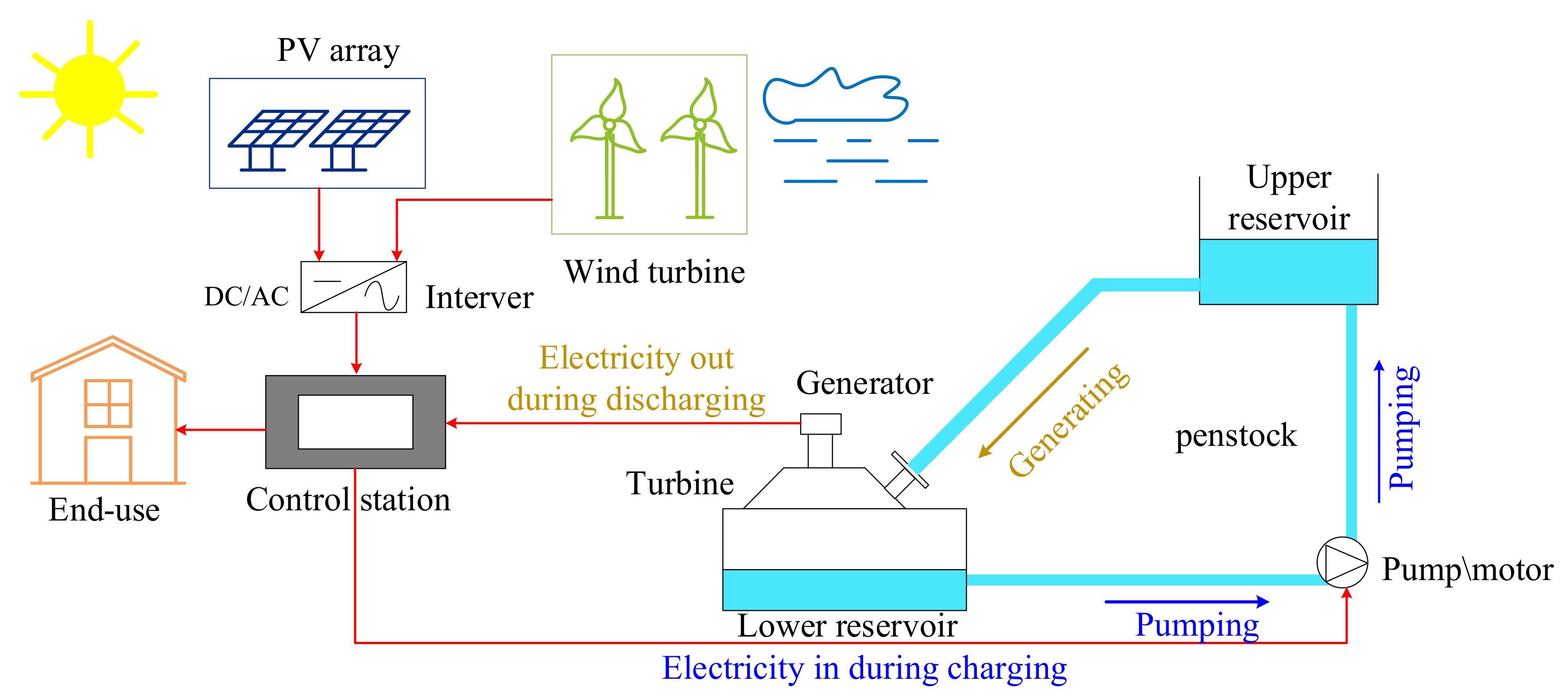
2.1. Model of the Pumped Storage Power Plant

2.1.1. Penstock

According to the IEEE group, the traveling wave transfer function between head and flow rate is written as [20]
h q = Z 0 q tanh ( T 0 s )
where T0 = L/α and Z0 = αQr/AigHr. hq is the relative value of head change caused by flow change. T0 is the elastic time of the equivalent penstock. α is the water hammer wave speed. L is the length of penstock. Z0 is the surge impedance in per unit of the equivalent penstock. Qr and Hr are the rated flow and head, respectively. Ai is the section dimension of the penstock. g is the acceleration of gravity. q represents the relative value of flow. s is the Laplace operator.
If we expand tanh(T0s) and omit the higher order term, then Equation (1) can be rewritten as [21]
h q ( s ) = Z 0 π 2 T 0 s + T 0 3 s 3 π 2 + 4 T 0 2 s 2 q ( s )

2.1.2. Hydraulic Speed Regulation System
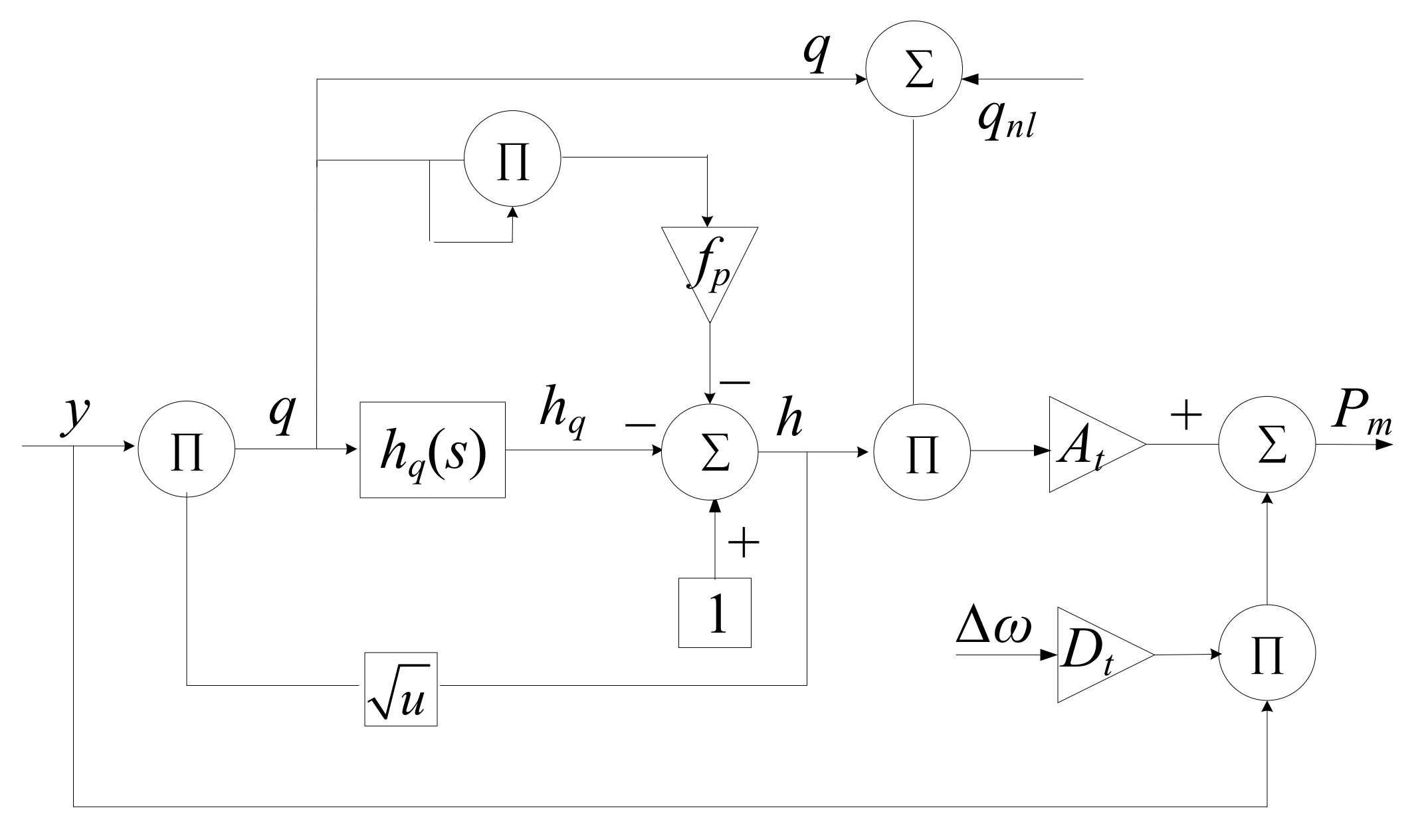
The servomotor is used to amplify the control signals and provide power to regulate the guide vane. The transfer function of the hydraulic servo system can be shown as [22]
G ( s ) = 1 1 + T y s
where Ty is the engager relay time constant.
A PID controller is commonly used. The transfer function of a PID can be expressed as [23]
G ( s ) = ( k p + k i s + k d s )
where kp, ki and kd denote the proportional, integral and differential adjustment coefficient, respectively.
Substituting Equation (4) into Equation (3), one can get
d y d t = 1 T y ( k p ω k i ω 0 δ k d d ω d t y )
where ω and δ are the relative value of the generator rotor speed and the relative value of the rotor angle, respectively. y is the relative value of the guide vane opening.

2.1.3. Turbine

The nonlinearity of the turbine has a great influence on the stability calculation of the power system. Thus, the nonlinear model is considered in this section. Due to the fact that the efficient of the turbine is not 100%, the algebra equation of the IEEE Working Group Model can be used to calculate the output of the turbine [20]:
p m = A t h ( q q n l ) D t y Δ ω
where pm stands for the power output of the hydro turbine per unit. At and qn1 denote the gain coefficient of the turbine and the no-loading flow per unit. Dt and Δω represent the mechanical damping coefficient of the hydro turbine and the difference of angular velocity, respectively.
The block diagram of the turbine is shown in Figure 2.

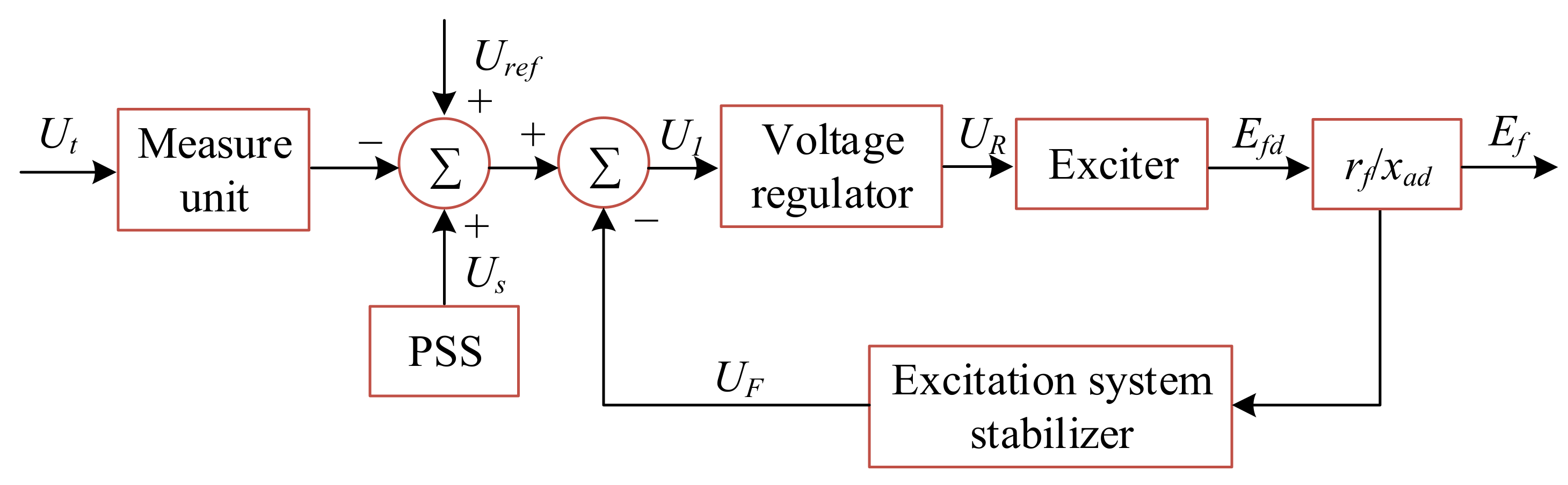
2.1.4. Excitation System
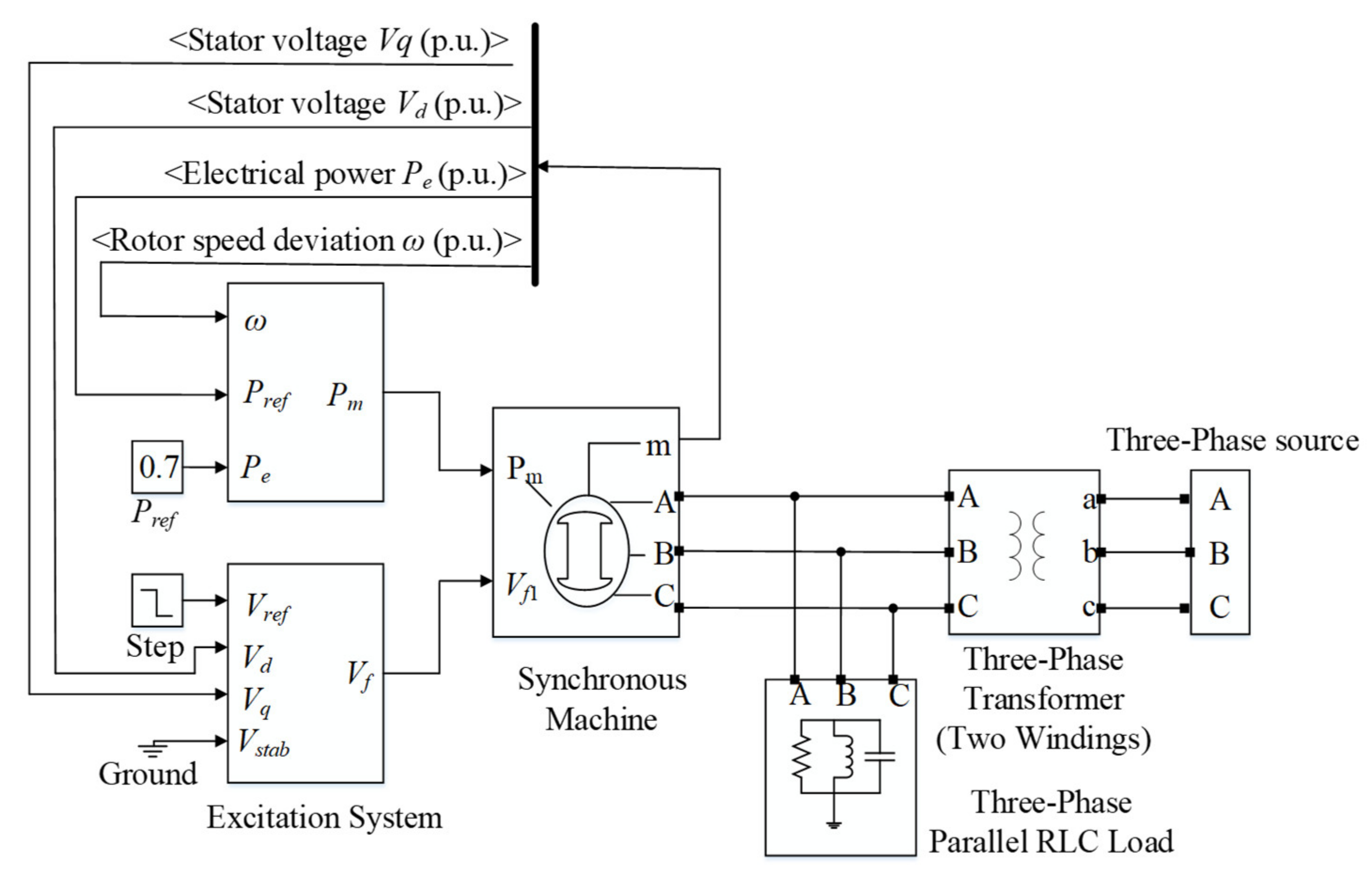
The stable operation of the power system is threatened due to the transient characteristics, such as sudden short-circuit faults [24]. The excitation system has the ability for additional damping to deal with these transients, which supplies a powerful guarantee for the safe and economical operation of the power system. Therefore, the excitation system is considered in this paper. A typical excitation system configuration is shown in Figure 3. The excitation system model of each unit is shown in Table 1.

2.1.5. Generator

A generator is the key component of the power system. First−order, three−order, five−order, and even seven-order generator models are commonly used to conduct research. However, it is a fact that the higher the model order, the higher the cost in terms of data requirements and calculation time [25]. Generally speaking, a third-order model has the advantage of simple structure and also considers the excitation system, which is widely used in dynamic analysis of the power system. Therefore, a third-order synchronous generator model is used in this paper, which is written as
d δ d t = ω B ( ω 1 ) d ω d t = 1 T j ( P m P G D t ( ω 1 ) ) d E q d t = ω B T d 0 X d X d E q + ω B T d 0 X d X d X d U s cos δ + ω B T d 0 E f
where δ, ω, and ωB are the rotor angle of the generator, the deviation of the relative angular speed and the nominal generator rotor speed, respectively. Pm and PG represent the hydro turbine output power and the generator magnetic power, respectively. Tj, Dt and T d 0 denote the inertia time constant of the generator, the generator damping coefficient and the generator time constant, respectively. Xd∑, X′d∑, Us and Ef stand for the d-axis synchronous reactance, the d-axis transient reactance, the bus voltage and the controller output, respectively.

2.1.6. Pumped Storage Power Plant Model

According to the above analysis, the block diagram of the pumped storage power plant model is shown as Figure 4. In Figure 4, a step disturbance is set to investigate the dynamic response of output variables of PSPP.

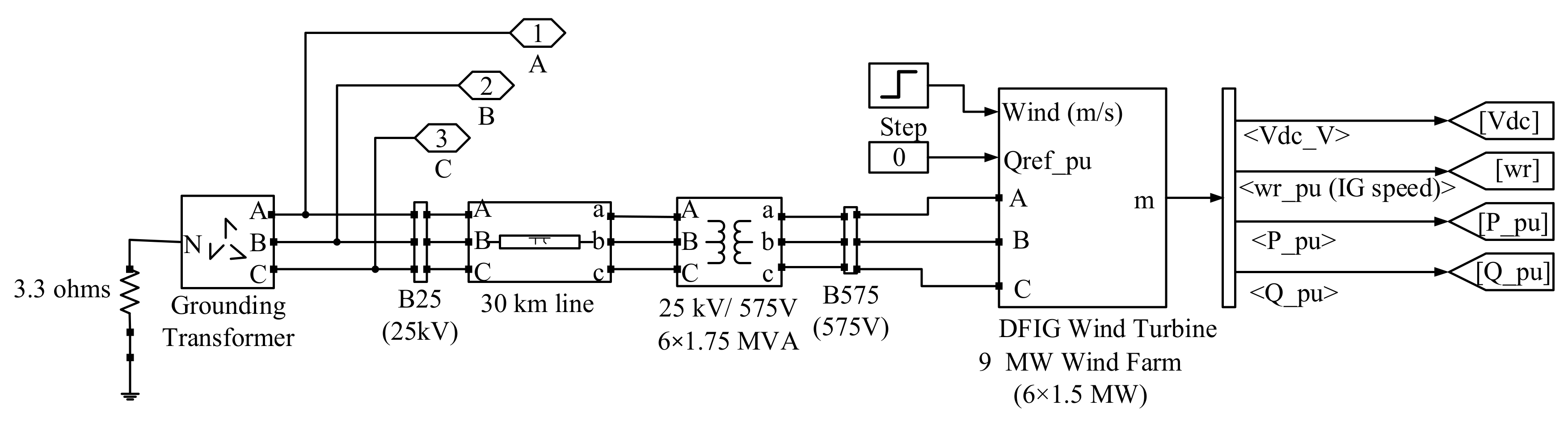
2.2. Wind Power Generation System (WPGS)

The wind power generation system consists of the wind turbine, drive train, generator, pitch blade servo system and AC–DC–AV converter. The Double Fed Induction Generator (DFIG) is widely used in the wind farm due to its excellent operating performance; that is, the WPGS with DFIG attains lower requirements for power converter capacity, and flexible regulation of active and reactive power. [26]. The DFIG is connected directly to the power grid of 50 Hz via its stator, while the rotor is connected to the power grid through a power converter. A wind turbine is a complex non-linear mechanical device [27], and it ensures the conversion of the wind energy into mechanical energy by coupling generator with wind turbine [28].
The power versus wind speed curves are written as [17]
P W T = 0 , 0 < v < v c i   or   v c o > v P r a t e d × ( A + B v + C v 2 ) , v c i < v < v r P r a t e d , v r < v < v c o
where PWT and Prated are the power output of a wind turbine and the rated electrical power, respectively. vci represents the cut−in wind speed. vr is the rated wind speed. vco stand for the cut−off wind speed. A, B and C are the intermediate variables, i.e.,
A = 1 ( v c i v r ) 2 [ v c i ( v c i + v r ) 4 v c i v r ( v c i v r 2 v r ) 3 ] ,
B = 1 ( v c i v r ) 2 [ 4 ( v c i + v r ) ( v c i + v r 2 v r ) 3 ( 3 v c i + v r ) ]  
and
C = 1 ( v c i v r ) 2 [ 2 4 ( 4 v c i + v r 2 v r ) 3 ] ,  
respectively.
Here, the wind farm cluster consists of 6 wind farms, each with a 1.5 MW wind turbine and a DFIGURE. It is connected to the external 25 KV AC grid through a 30 km and 25 KV transmission cable with the nominal power rating of 9 MW. The main purpose of this paper is to investigate the parameter uncertainty on the regulation performance of PSPP in a hybrid system. In order not to increase plant cost, the number of wind turbines and wind speed types remains unchanged. The WPGS model based on MATLAB/Simulink is shown in Figure 5.

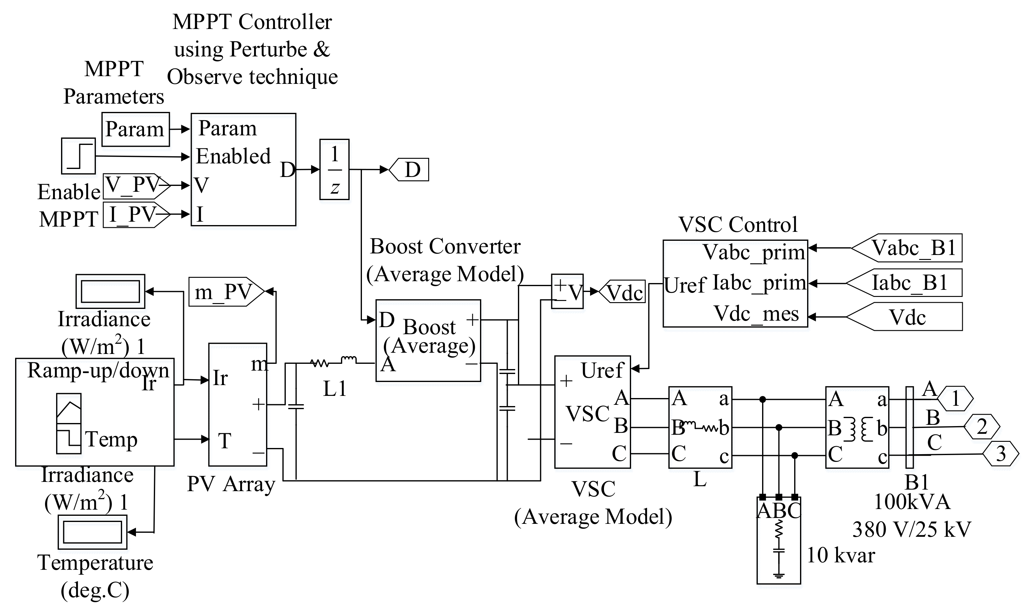
2.3. Photovoltaic Power Generation System (PPGS)

Being environmentally friendly, solar energy has become one of the most suitable renewable energies [29], which is used in various ways and has the potential to be an alternative to conventional energy resources [30]. The most common application form of solar energy is photovoltaic power generation (PPG) [31]. A typical solar photovoltaic generator system consists of solar panel, DC/DC and DC/AC converter and the associated control. The key specifications of the solar panels are presented in Table 2.
The relationship between the current and voltage of a PV cell is expressed as [19]
I = I p h I 0 ( e V + I R S V t 1 ) V + I R S R p
where Iph is the photo current. I0 is the diode saturation current. R′s is the series resistance. R′p is the shunt/parallel resistance. Vt is the diode thermal voltage.
The power output from a PV array is
P A = I A V A = N P I p h V A N P I 0 V A ( e 1 V t ( V A N s + I A N p R s ) 1 ) N P R p V A ( V A N s + i A N p R s )
where NS and Np are the number of PV cells in a series for the studied array and the number of PV module in parallel, respectively. PA, IA and VA are the power output, current and voltage of a PV array, respectively.
Due to the nonlinear photovoltaic cell array, the related controller is considered to maintain the photovoltaic power generation efficiency. Based on the above consideration, a generic model of PPGS developed in MATLAB/Simulink software is shown in Figure 6.

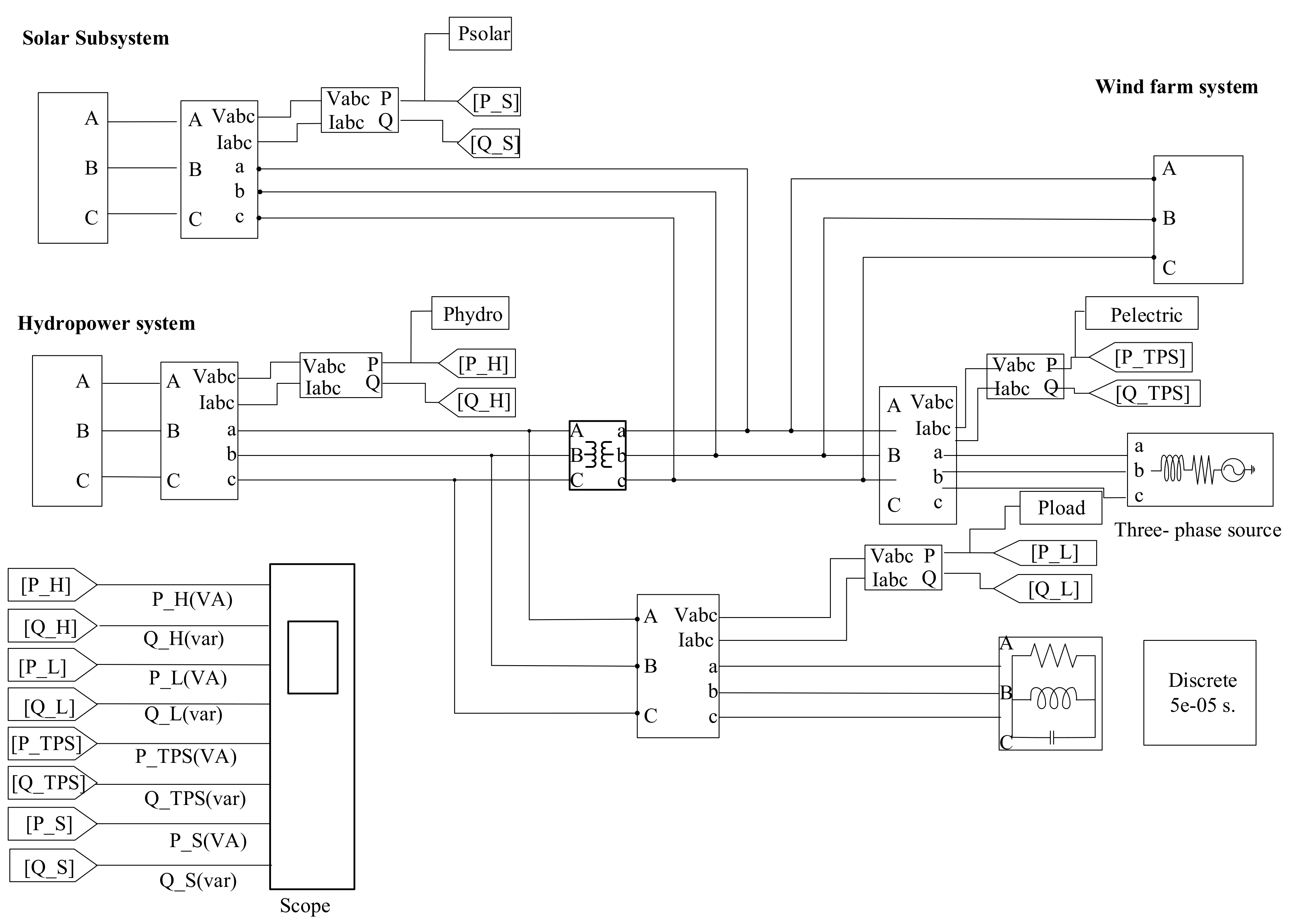
2.4. Model of the Wind−Solar−Hydro Hybrid System

According to the above analysis, the proposed WSH hybrid system schematic is demonstrated in Figure 7. Please see Ma et al., for more detailed information about the operating principle of the hybrid system [19].
This section supplies an interface to connect the wind, solar and hydro system model, which poses a potential reference to the multi−energy complementary system to better use clean energy.

2.5. Uncertainty Analysis

The mathematical model is crucial to simulate, study and predict the output of the WSH hybrid power generation system. The hybrid system model is complex, with nonlinear relations and many parameters. The important characteristic of these parameters is uncertainty, which has the ability to lead to the output uncertainty of the system [32]. Therefore, it is of importance to identify the relevance of these uncertainty parameters for the model.
One should note that uncertainty analysis often involves a larger number of parameters and data [33]. However, data of most parameters are generally very scarce and cannot be measured directly, which significantly affects the analysis results. Therefore, it is necessary to generate a large amount of random data within an acceptable range using a random sampling method. The Monte Carlo method has become a practical random sampling since it is simple, model-independent and generally applicable [32]. Please refer to Iooss and Le Gratiet (2019) for detailed information on the Monte Carlo method [34].

2.6. Sensitivity Analysis

The sensitivity analysis method is a valuable tool for building and using numerical simulation models [35]. It is used to study the influence of parameters uncertainty on the system output by setting the variation of model parameters in the corresponding design space [36]. Through sensitivity analysis, the model correction can set the parameters with low sensitivity to fixed values, and only calibrate the parameters that have great influence on the output variables, thus effectively simplifying the model, and improving the calibration accuracy of the model and saving time [37]. The first historical approach to sensitivity analysis is known as the local sensitivity where the effect of small input disturbance occurred around nominal values on the model output is studied [38]. To overcome the limitations of local methods (linearity and local variations), global sensitivity analysis considering the whole variation range of the inputs was developed in the late 1980s [35]. The extended Fourier amplitude sensitivity test (EFAST) is one of the most commonly used global sensitivity analysis methods, since it studies the influence of each parameter and the interaction of parameters on system output when multiple parameters change simultaneously [39]. Please see Xu et al., for detailed information about EFAST [40].

2.7. Reliability Analysis

Reliability analysis is usually performed when a structure is subject to uncertain influences [41]. The reliability, defined as the probability of the structure in a safe state, is
R = S p ( x ) d x = 1 F p ( x ) d x
where S and F′ represent the state domain and the failure domain, respectively. The surface separating S and F’ is called the failure surface or limit state surface. x represents the possible value of the uncertain component.
At present, the commonly used reliability calculation methods are the first-order reliability method (FORM), second-order reliability method (SORM), Monte Carlo method (MCS) and so on [42]. FORM is a popular one due to its simplicity, since only second moment information and the probability distribution type of the random variables are required to estimate the probability [43]. Based on the reliability indicators and checking points of the FORM, the SORM uses the second-order Taylor series expansion at the checking point to replace the original functional function, so as to improve the calculation accuracy of the FORM.

2.7.1. First-Order Reliability Method

The matrix formulation for a correlated normal of the Hasofer–Lind index (β) (also called first-order reliability index) can be expressed as [44]
β = min x F ( X μ ) T C 1 ( X μ )
where X stands for the vector representing the set of random variables xi. μ, C and F are the vector of mean values, the covariance matrix and the failure domain, respectively.
Low and Tang [45,46] presented an alternative interpretation of β based on the perspective of an expanding ellipsoid in the original space of the basic random variables, expressed as follows:
β = min x F x i - μ i N σ i N T R - 1 x i - μ i N σ i N
where [R] stands for the correlation matrix. μ i N denotes the equivalent normal mean. σ i N is the equivalent normal standard deviation of random variable xi.
Based on the reliability index, the probability of failure can be evaluated as follows
P f 1 φ β
where φ(β) refers to the cumulative distribution function of the standard normal variable. Pf is the probability of failure.

2.7.2. Second-Order Reliability Method

The SORM of the response surface g ˜ ( u ) = 0 is given by second-order Taylor series expansion at the design point u* in a standard normal U-space as [43]
g ˜ u α T u u * + 1 2 u u * T B u u *
where α = g ˜ u g ˜ u , B = 2 g ˜ u g ˜ u . α is the directional vector at the design point in U-space. B is the scaled second-order derivatives of g ˜ ( u ) at u*, known as the scaled Hessian matrix.
The symbols used in this paper are shown in Table 3.

3. Numerical Experiments

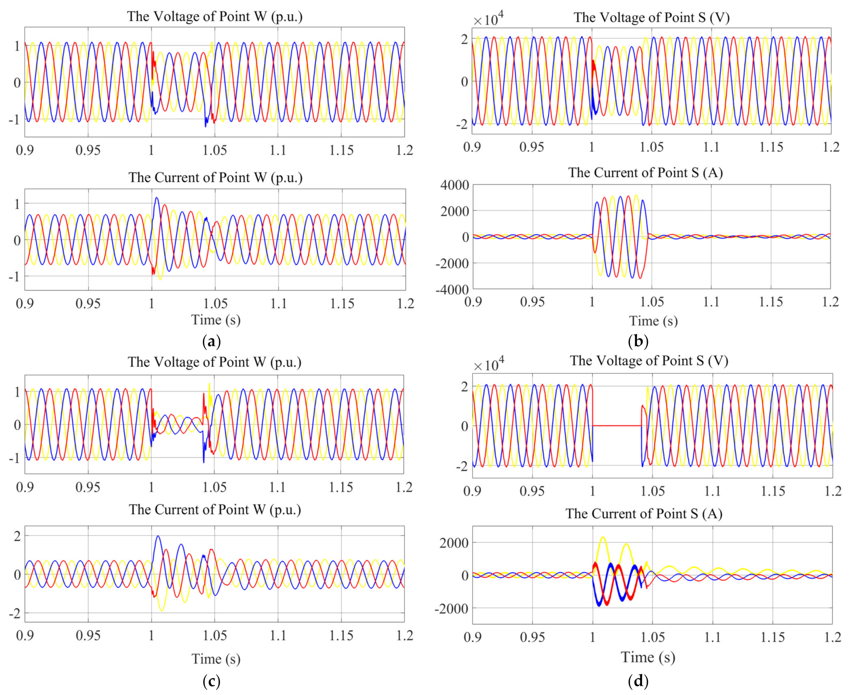
3.1. Dynamic Characteristics of WSH System in Steady and Fault States

In the hybrid power system model, two fault points, i.e., H and S, are set up at the output terminal of PSPP and infinite power supply to simulate the situation of the three−phase short circuit fault (TPSCF). The fault occurs at 1 s, is resected at 1.04 s, then the system gradually returns to normal operation. Meanwhile, the three−phase voltage and current of the output terminal of Wind Power Generation (WPG) (labeled as W) and grid-side (labeled as S) are measured, respectively. The corresponding numerical experiments are shown in Figure 8.
Figure 8a,b demonstrate the dynamic characteristics of a three-phase current and the voltage of points W and S with a three-phase short circuit fault of point H occurring at 1.0 s and being removed at 1.04 s, respectively. From Figure 8a,b, it can be seen that the three−phase voltage and current are in a stable periodic motion when t < 1 s. With TPSCF occurring, the three−phase voltage of points W and S decreases, while the three-phase current of points W and S increases. The three−phase voltage and current of each point return to normal values and finally reach a stable state after the fault is removed at t = 1.04 s. Figure 8c,d illustrate the dynamic characteristics of three−phase current and voltage of points W and S with a three−phase short circuit fault of point S occurring at 1.0 s and being cleared at 1.04 s, respectively. From Figure 8c,d, the three-phase voltage and current of each point spread in a stable periodic motion when t < 1 s. The three-phase voltage of points W and S decreases significantly, while the three-phase current of points W and S increases between t = 1 s and t = 1.04 s. Specially, the three−phase voltage of points W and S returns to its normal value and finally reaches a stable state after the TPSCF is removed. The three−phase current of points W and S transforms from the periodic motion to an undulant state during the TPSCF. It worth noting that one of the three−phase currents of point S is separated from the others during the TPSCF. After the TPSCF is removed, the three−phase current of point W rises to its normal value and finally reaches a stable state. However, one of the three−phase currents of point S is still separated from the others, while the others finally return to a stable state.
The above simulation results have proved that the established model is feasible which can be used to study the reliability analysis of the wind–solar–hydro hybrid power generation system in the following subsections.

3.2. Dynamic Performance Indexes (DPIs)

The response quality of the system under disturbance is usually measured by a dynamic performance index of the output variable. It is of practical significance to study the dynamic characteristics of the system by discussing the relationship between the DPIs and the system parameters. The commonly used DPIs are rise time (tr), settling time (ts), peak value (p), peak time (tp) and overshoot (Os), which are used to characterize the response rapidity and stability of the system. Please refer to Appendix A for more details about DPIs. The corresponding results of the DPIs with Ke and Ki changing are shown in Table 4 and Table 5.
Table 4 shows the statistics of the DPIs of the reactive power and generator terminal voltage with Ke and Ki changing. As for the DPIs of the reactive power, it can be seen that the difference in rise time between different Ke and Ki settings is relatively small compared with that of settling time. The peak value and peak time remain almost unchanged with Ke or Ki changing. Settling time increases with the increases of Ke with a fixed Ki, while rise time shows the opposite trend. The maximum and minimum of settling time are 1.39728 and 0.70833, respectively. It worth noting that Ki has little effect on the DPIs of the reactive power when Ke remains unchanged. With regard to the DPIs of the generator terminal voltage, Ke has influences on the rise time, settling time, peak value and overshoot with different degrees. Specifically, with the increases of Ke, the rise time and peak value decrease, the settling time and overshoot values increase, while the peak time remains unchanged. When Ke = 8, the settling time and overshoot reach the maximum 1.9153 and 2.46662, meaning that a larger Ke value results in a poor rapidity and stability of the system response. The best overall quality of regulation occurs in Ke = 6 which has a relatively smaller settling time and overshoot. In addition, there is little change in the rise time, settling time, peak value, peak time and overshoot with Ki changing, which means that Ki has almost no effect on the DPIs.
Table 5 displays the statistics of the DPIs of the guide vane opening and angular velocity with Ke and Ki changing. From Table 5, Ke and Ki have little influence on the rise time, settling time, peak value and peak time of the guide vane opening since the difference in each DPI result between different Ke and Ki settings is relatively small. However, the overshoot values of the guide vane opening decrease with the increases of Ke and Ki. The maximum and minimum of the overshoot of the guide vane opening are 189.362 and 181.57, occurring in simulation No. 16 and No. 12, respectively. That is to say that a smaller setting of Ke and Ki causes a slower governor movement, leading to a larger overshoot of the guide vane opening. The above results show that the different Ke and Ki settings have a significant influence on the regulation quality of the guide vane opening. As for the DPIs of the angular velocity, it can be seen that both Ke and Ki have almost no effect on rise time, peak value and peak time. The maximum of settling time occurs in simulation No. 16 where Ke = 6 and Ki = 0.1. In addition, the values of overshoot at Ke = 6 are larger than those at Ke = 7 and Ke = 8. This means that the greater Ke value is, the better the dynamic performance of the system is.

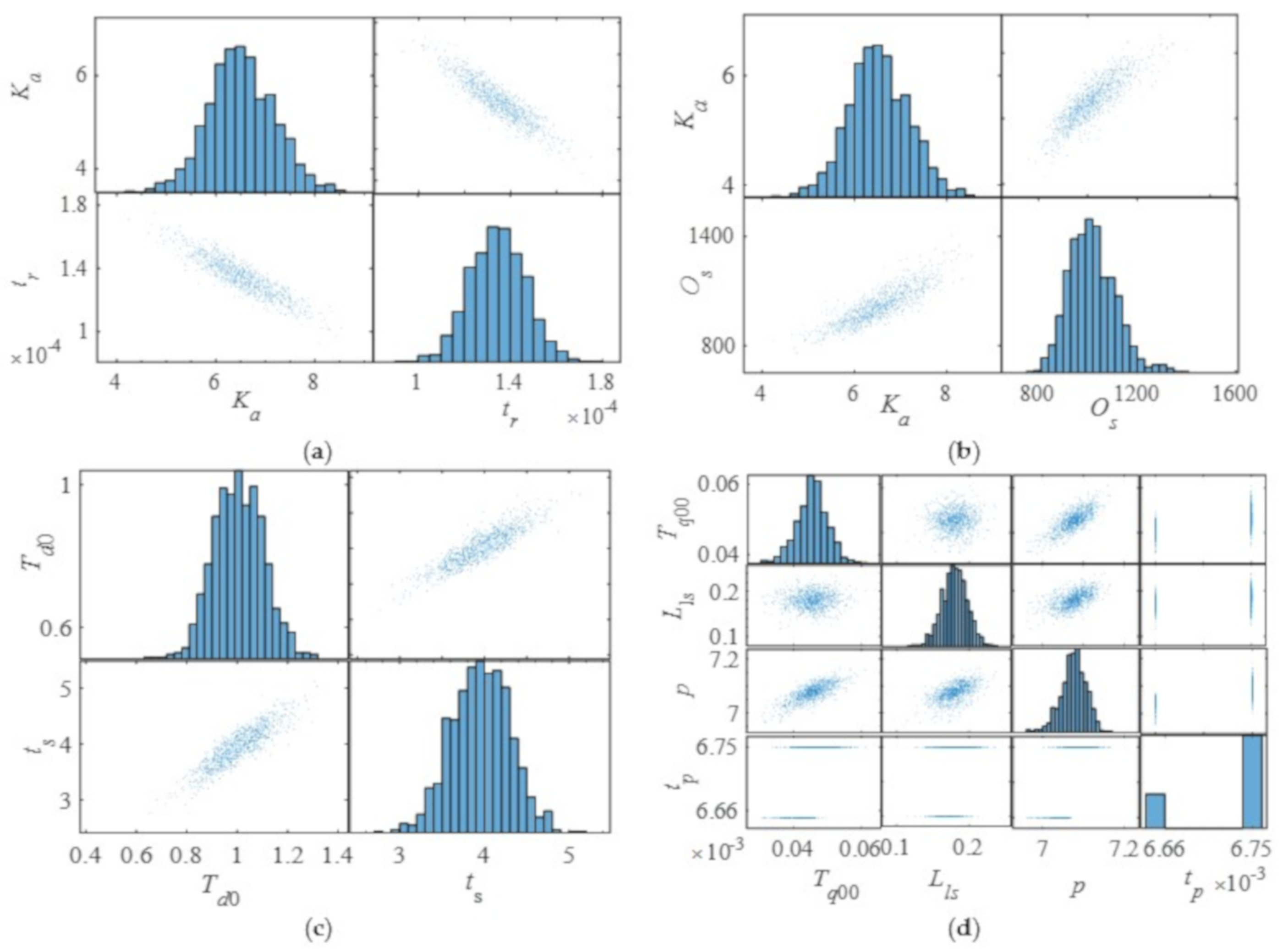
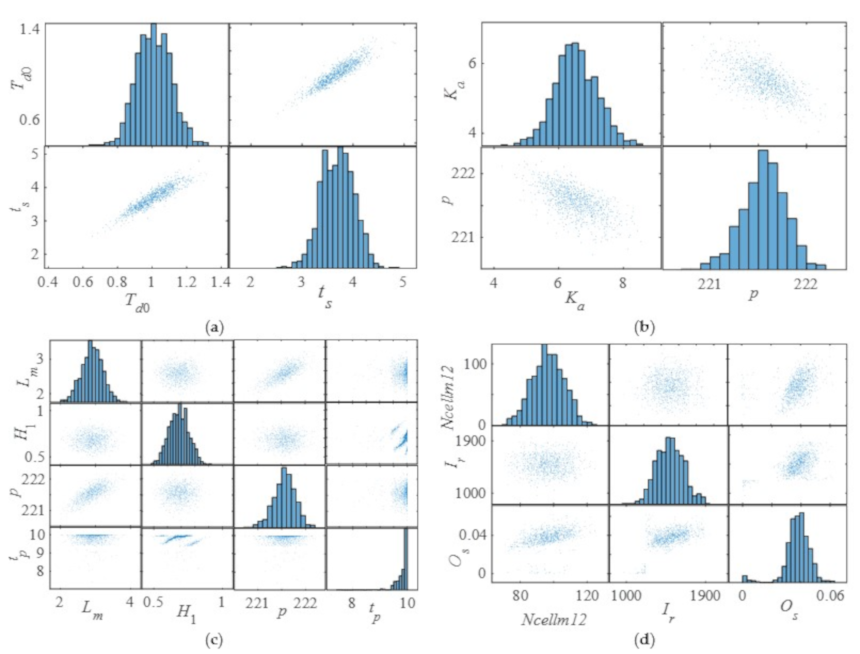
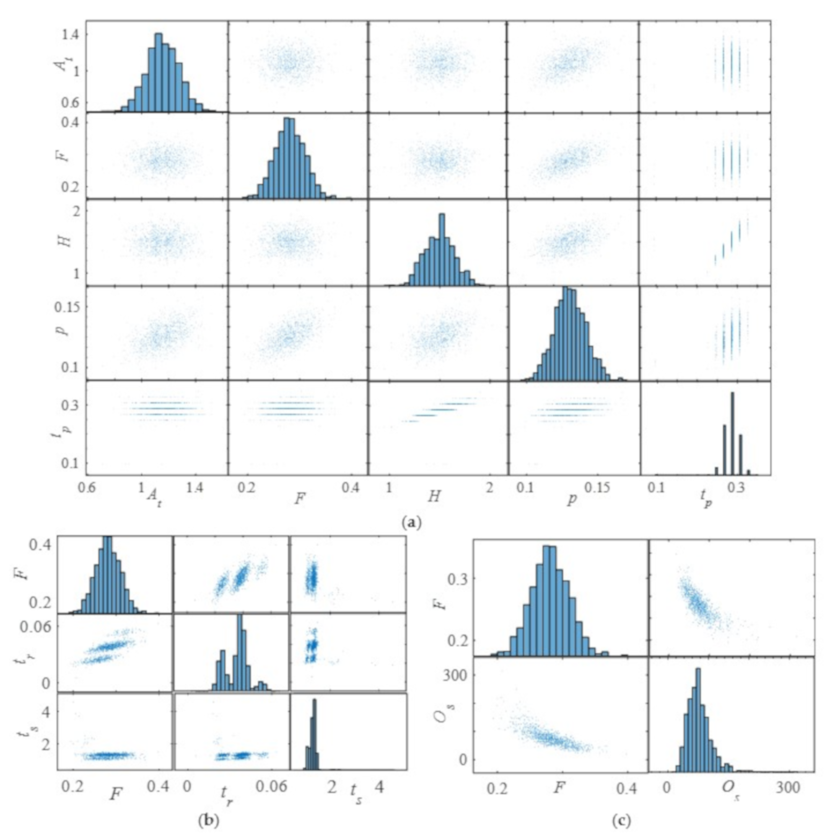
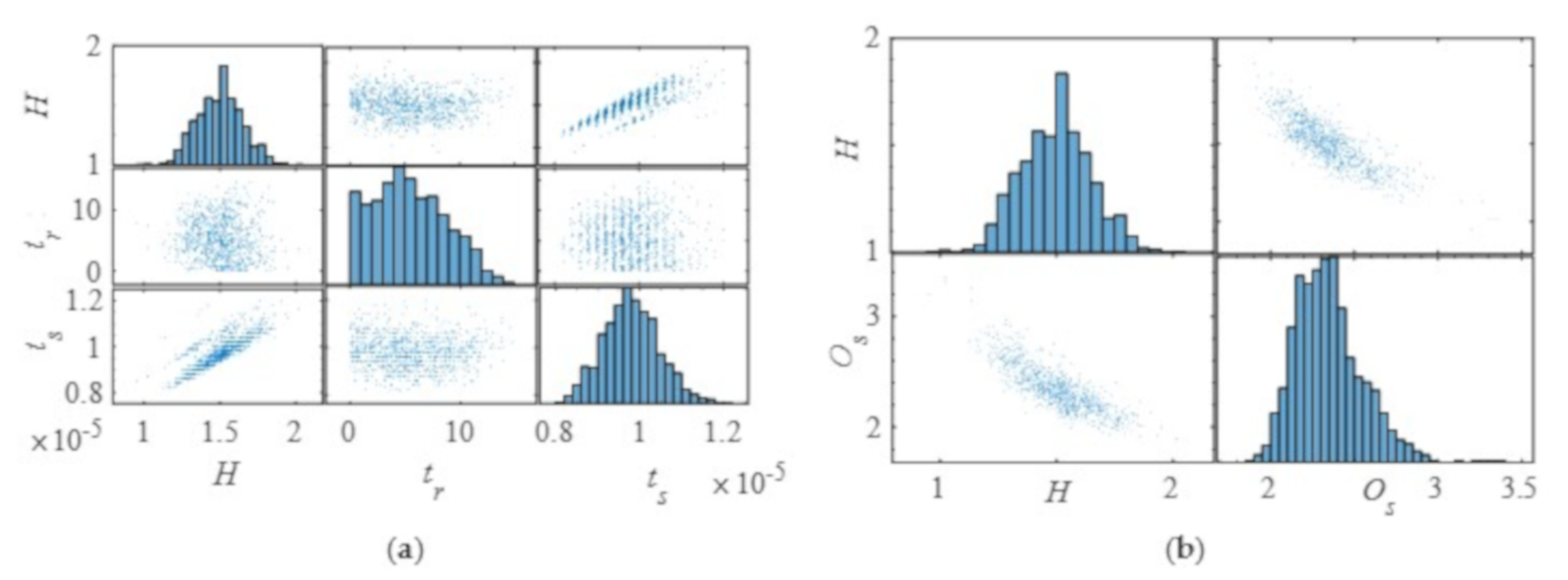
3.3. Uncertainty Analysis

In this section, the Monte Carlo method is used to analyze the influence of WSH parameters on the output of PSPP. The iteration step is 1000, and the initial values of Ke and Ki are 7 and 0.25, respectively. Other parameters are set to conform to the normal distribution as shown in Appendix B. For the sake of brevity, only the parameters with definite influence rules on the output of PSPP are given. Graphics on diagonal lines indicate that the values of system parameters are in accordance with the normal distribution. The corresponding numerical results are shown in Figure 9, Figure 10, Figure 11 and Figure 12.
Figure 9 demonstrates the influence of WSH system parameters on the DPIs of the reactive power of PSPP. More specifically, Figure 9a is the influence of Ka on the rise time. Figure 9b is the influence of Ka on the overshoot. Figure 9c is the influence of Td0 on the settling time. Figure 9d is the influence of Tq00 and L1s on the p and pt. From Figure 9a, the rise time decreases with the increases of Ka. The overshoot shows an opposite trend compared with that of the rise time; that is to say that the overshoot increases with Ka increasing as shown in Figure 9b. Figure 9c shows that the settling time increases with Td0 increasing. From Figure 9d, with the increases of Tq00 and Lls, the peak value increases. However, the value of the peak time is discontinuous, that is, it always equals 0.00666 or 0.00675 regardless of what the parameters are. The above results show that both parameters of PSPP and WPGS have a deterministic effect on the DPIs of reactive power, while PPGS parameters have no regular influence. In other words, WPGS has the ability to regularly affect the DPIs through the coupling effect of subsystems.
Figure 10 shows the influence of WSH system parameters on the DPIs of the generator terminal voltage of PSPP. Figure 10a is the influence of Td0 on the settling time. The changing trend of settling time is consistent with that of Td0, that is, the value of settling time increases with Td0 increasing. The changing trend of the peak value is decreasing as Ka increases in Figure 10b. Figure 10c shows the influence of Lm and H1 on the peak value and peak time. From Figure 10c, the peak value of the generator terminal voltage increases with Lm increasing. No matter how Lm and H1 change, the maximum peak time does not exceed 10. From Figure 10d, the value of overshoot rises due to the increases of Ncellm12 and Ir, indicating that the larger the capacity of photovoltaic power generation is, the greater the adverse effect on the voltage stability. From Figure 10a–d, parameters of WPGS, PSPP, and PPGS have regularity impacts on DPIs of the voltage. That is to say that WPGS and PPGS have a regular impact on the terminal voltage due to the coupling of subsystems.
Figure 11 presents the influence of parameters of WSH on the DPIs of the guide vane opening of PSPP. Figure 11a reveals the changing rules of peak value and peak time with At, F and H changing. The influence of At and F on the peak time are similar, that is, peak time presents a state of discontinuity strip-shaped on the vertical axis. The value of the peak time on each of the strip-shaped is constant. The increase of H leads to the increase of peak time, and the characteristics of peak time distribution are mainly strip-shaped on the vertical axis. The values are concentrated between 0.2 and 0.3. The peak value has a slight increasing trend with the increase of At, F and H. Figure 11b–d are the influence of F on the rise time and overshoot. From Figure 11b, F affects the value of rise time, and the distribution of rise time is concentrated between 0.02 and 0.05. Most of the settling time values are less than 1.5. Figure 11c shows that the value of overshoot decreases when the values of F increase. From the above analysis, it can be seen that the influence rule of different parameters is different due to parameter uncertainty. Meanwhile, only the uncertain parameters of PSPP show certainty influence on the DPIs of guide vane opening, which means that parameters of wind and solar subsystems have no regular influence on guide vane opening.
Figure 12 shows the influence of WSH parameters on the DPIs of the angular velocity of PSPP. Specifically, Figure 12a,b are the influence of H on the rise time, settling time and overshoot of angular velocity, respectively. The values of overshoot are decreasing gradually with H increasing, while the values of settling time are increasing gradually with the increases of H. The above results show that only uncertainty parameter H has a regular effect on the DPIs of the angular velocity of PSPP. In other words, WPGS and PPGS have no regular influence on the angular velocity compared with that of PSPP.
From the analysis of Figure 9, Figure 10, Figure 11 and Figure 12, different subsystems show different influence on the DPIs of PSPP output. It also can be obtained that the effects of PSPP parameters on each DPI have a certain regularity, while the influence degree of each PSPP parameter is different. This is due to the fact that system parameters are uncertain, and DPIs of this paper mainly depend on PSPP. The above results mean that to better maintain the regulation of PSPP, it is important to consider parameters’ uncertainty and the coupling effect of subsystems.
To reveal the response speed of the WSH system, the cumulative probability distribution of rise time and settling time are studied in the following contents. The sampling times are 1000 times. The corresponding numerical results are shown in Figure 13 and Figure 14.
Figure 13a–d shows the cumulative probability distribution for the rise time of reactive power, generator terminal voltage, guide vane opening and angular velocity, respectively. From Figure 13a, it can be seen that the cumulative probability of rise time of reactive power changes as an “S” curve. No matter what the system parameter values are, the cumulative probabilities are 1.273% and 98.61% with the value of the rise time less than 1.101 × 10⁻⁴ and 1.599 × 10⁻⁴. These phenomena mean that most of the rise time values are less than 1.599 × 10⁻⁴. From Figure 13b, the cumulative probability curve is relatively steep, indicating that the rise time value of the generator terminal voltage is comparatively centralized. The cumulative probability of rise time values less than 0.1406 is 99.34%, while the cumulative probability is almost equal to 0 with rise time value less than 0.08581. That is to say that the rise time value is in the range of 0.08581 and 0.1406. From Figure 13c, the cumulative probability is 99.62% when tr < 0.05674, and the cumulative probability is 0.4066% when tr < 0.01501. From Figure 13d, most of the values of rise time are less than 1.468 × 10⁻⁴, where the cumulative probability is 99.41%. Meanwhile, the slope of rise time cumulative probability of angular velocity curve changes smoothly compared with that of reactive power, generator terminal voltage and guide vane opening. The above phenomena show that there are great differences in the rise time of different output variables, especially reactive power and angular velocity. The cumulative probability curve in Figure 13b changes faster than those in other subgraphs.
Figure 14 shows the cumulative probability distribution for the settling time of the reactive power, generator terminal voltage, guide vane opening and angular velocity. It can be seen that all the cumulative probability curves are similar to “S”. The slope of the cumulative probability curve of the angular velocity is larger than that of the reactive power, generator terminal voltage, guide vane opening; that is, the settling time distribution of angular velocity is relatively concentrated. Specifically, when ts < 1, the cumulative probability of angular velocity is larger than that of reactive power, generator terminal voltage and guide vane opening. When ts < 1, the cumulative probabilities of reactive power, generator terminal voltage, guide vane opening and angular velocity are 0, 0, 0.3797% and 66.58%, respectively. When ts < 2, the cumulative probabilities of reactive power, generator terminal voltage, guide vane opening and angular velocity are 0, 0, 99.83% and 100%, respectively. When ts < 4, the cumulative probabilities of reactive power, generator terminal voltage, guide vane opening and angular velocity are 54.91%, 82.48%, 100% and 100%, respectively. From the comparative results, the possible value of the settling time of the guide vane opening and angular velocity are larger than that of reactive power and generator terminal voltage in the case of large probability. The cumulative probability distribution of reactive power, generator terminal voltage, guide vane opening and angular velocity is significantly different from each other.
From Figure 13 and Figure 14, for the same DPI, the cumulative probability distributions of different output variables are significantly different from each other. This is because system parameters have different influences on system output as discussed in Section 3.3. Regarding different DPIs, the cumulative probability distributions of the same output variable are also different. In general, the settling time is larger than the rising time. This is due to the fact that the rise time is the time required for the response curve to reach the steady value for the first time, while the settling time is the time when the error between the unit step response and the steady value reaches the accepted value. In other words, the combination of Figure 13 and Figure 14 can more clearly reflect the response speed of the system after disturbance.

3.4. Sensitivity Analysis

The sensitivity of model parameters often leads to the uncertainty of the model simulation. Therefore, finding out the sensitive parameters is significant to study the influence of effective parameters on the model output variables. Here, the Extended Fourier Amplitude Sensitivity Test (EFAST) method is used to study the sensitivity. The change law of system parameters is set to normal distribution as shown in Appendix B. The Monte Carlo method is selected for parameter random sampling, and the sampling times are 1000 times. The corresponding results are shown in Figure 15, Figure 16, Figure 17, Figure 18 and Figure 19 and Table 6.
Figure 15 shows the sensitivity index of parameters of the rise time of angular velocity. Specifically, Figure 15a,b display the sensitivity index of 25 parameters and the top 10 parameters of rise time of the angular velocity, respectively. From Figure 15a, the 25 parameters have different effects on the angular velocity. To visualize the sensitivity scenarios, the top 10 sensitive parameters are plotted in Figure 15b, where these parameters have a relatively large impact on the rise time. The numerical results are shown in Table 6. From Figure 15b and Table 6, T0 has the strongest impacts on the rise time of the angular velocity with sensitivity index 56.99%, followed by H1 (9.298%), Ir (2.859%), Dt (2.719%), Tq00 (2.144%), Ncellm12 (1.878%), bp (1.51%), Kd (1.507%), T (1.478%) and qnl (1.388%). The total contribution rate of the top 10 sensitive parameters is 81.77%, meaning that these parameters have a direct effect on the rise time of angular velocity and the most significant factors affecting the rise time are identified through sensitivity analysis. The contribution rate of other parameters is less than 1.3%, indicating that the sensitivity of interaction among these parameters is small and the parameters are independent. In addition, it is worth noting that the second and the third sensitivity parameters are H1 and Ir coming from WPGS and PPGS, respectively. These phenomena mean that these parameters have the ability to indirectly influence the angular velocity of PSPP by interacting with other parameters.
Figure 16 demonstrates the sensitivity index of parameters of the settling time of angular velocity. From Figure 16a, it can be seen that different system parameters affect the settling time to a different degree. There are 10 sensitive parameters that have a relatively greater influence on settling time, as shown in Figure 16b and Table 6. Specifically, H has the greatest influence on settling time with sensitivity index 33.7%. The others are Tq00 (22.29%), At (4.851%), F (3.619%), Kp (1.829%), H1 (1.674%), Rr (1.671%), F1 (1.645%), Ka (1.596%) and Rs (1.57%). The total contribution rate of the top 10 sensitive parameters is 74.45%, meaning that the most significant factors affecting the output are studied and identified through sensitivity. Therefore, the influence of the top 10 sensitive parameters on the settling time should be fully considered in the numerical simulation of the WSH hybrid system. The sensitivity index of other parameters is less than 1.6%, indicating that the sensitivity of interaction among these parameters is small and the parameters are independent.
Figure 17 shows the influence degree of parameters on the peak value of the angular velocity. Figure 17a shows the impact of 25 parameters on the peak value of the angular velocity. The top 10 sensitive parameters that have a relatively larger influence on the peak value are shown in Figure 17b. The corresponding results including the sensitivity index and the sensitivity ranking are shown in Table 6. From Figure 17b and Table 6, the most sensitive parameter is H with a contribution rate 72.55%, indicating that the H value directly determines the peak value of the angular velocity. Therefore, more attention should be paid to H to main the system stability. The second one is At with a sensitivity index 5.44%, followed by F, Tq00, qnl, Ka, Rs, Td00, H1 and Kp with sensitivity index 2.693%, 2.663%, 2.073%, 2.053%, 1.779%, 1.581%, 1.333% and 1.286%, respectively. The total contribution rate of the top 10 sensitive parameters to the peak value is 93.45%, which indicates that these parameters have a significant influence on the peak value of the angular velocity.
Figure 18 displays the contribution rate of different parameters on the uncertainty of peak time of the angular velocity. Figure 18a is the main effect of the 25 parameters on the peak time of the angular velocity. Figure 18b shows the top 10 sensitive parameters that have a greater impact on the peak time. Rankings of the top 10 sensitive parameters are shown in Table 6. From Figure 18b and Table 6, the sensitivity ranking is H, T0, Ncellm12, Tq00, Lls, Ka, T, Rs, Ir and At. The corresponding sensitivity indexes are 71.59%, 2.355%, 2.231%, 1.988%, 1.844%, 1.681%, 1.444%, 1.422%, 1.318% and 1.28%, respectively. The total contribution rate of the top 10 sensitive parameters is 87.15%, that is, the top 10 sensitive parameters have a significant influence on the peak time of the angular velocity. In other words, the influence of different parameters on peak time varies greatly. The Ncellm12 is the third sensitivity parameter coming from PPGS, indicating that the parameter of PPGS has the ability to indirectly affect the angular velocity by interacting with other parameters. In addition, H has the greatest impact on the peak time consistent with that of peak value and settling time, indicating that the most sensitive parameters of these DPIs are consistent.
Figure 19a,b describe the main effects of 25 parameters and the top 10 sensitive parameters on the overshoot of the angular velocity, respectively. The top 10 sensitive parameters are T0, qnl, Rs, Lm, Ncellm12, H1, Kd, fp, Ir and H, respectively. The sensitivity results are shown in Table 6. From Table 6, the maximum sensitivity index is 3.177% coming from T0, and the minimum sensitivity index is 1.328% coming from H. It also can be seen that the total contribution rate of the top 10 sensitive parameters is 17.764%. It is worth noting that the sensitivity index value is relatively small compared with that of rise time, settling time, peak value and peak time. This phenomenon means that although many factors affect the overshoot of angular velocity, the difference of influence degree is small.
From Figure 15, Figure 16, Figure 17, Figure 18 and Figure 19 and Table 6, it is concluded that the sensitivity degree of different DPIs to system parameters is obviously different. This phenomenon means that even the same parameter has a different effect on the response speed and response stability of the system. Moreover, parameters of WPGS and PPGS have a significant influence on DPIs, indicating that these parameters have the ability to indirectly affect the angular velocity of PSPP by interacting with other parameters.

4. Reliability Analysis

The regulation reliability of WSH hybrid power generation system is directly related to the balance between the power supply and demand. Therefore, it is of great significance to study regulation reliability to maintain the safe and economic operation of the power system. In this section, we study the influence of the system parameters on the output of the WSH system. Here, the peak value of angular velocity is selected as an example, and the number of simulations is 2000.
Figure 20 is the distribution of the peak value of angular velocity. From Figure 20, the abscissa represents the peak value of angular velocity, which is distributed between 0.017 and 0.034. The ordinate stands for the number of corresponding peaks. It is clear that the peak value of angular velocity approaches the normal distribution well. Most of the peak values are in the range of 0.022 and 0.024, and the values on both sides are relatively small. Here, the peak value greater than 0.028 is defined as failure range. According to this definition, some values in Figure 20 are in the failure range, and the probability of this part is called the failure probability. To avoid the peak value falling in the failure range, the system parameters should be adjusted based on the results of uncertainty analysis and sensitivity analysis to meet the steady state operation. In addition, the cumulative probability diagram is plotted in Figure 21 to obtain the failure probability.
Figure 21 demonstrates the cumulative probability of the peak value of the angular velocity. The blue solid line is the cumulative probability curve for the peak value, and the red dashed line is the 95% confidence bounds. From Figure 21, it can be seen that the blue solid line is within the 95% confidence bounds, meaning that the simulation results are proved to be reliable. In addition, the cumulative probability of the peak value less than 0.028 is 97.5%, that is, the reliability probability of the power supply is 97.5%. In other words, the probability that the primary objective ensuring the balance between supply and demand cannot be satisfied is 2.5%, meaning that consumers cannot receive the electricity they need. This case may overburden the power system, cause widespread power blackout and finally pose a threat to the safe and economic operation of the power system.

5. Conclusions

To investigate the regulation reliability of PSPP in a multi-energy power system, a wind-solar-hydro hybrid power system model is established. Based on the established model, uncertainty and sensitivity analysis of system parameters were carried out using the Monte Carlo method and EFAST. Finally, the regulation reliability of the pumped storage power plant in a WSH hybrid power generation system was also discussed. The main results are as follows:
(1)
The influence rules of the model parameters on the WSH hybrid system are obtained from the uncertainty analysis. Parameters of the wind, solar and hydro subsystem show the different influence on DPIs of the PSPP output due to parameters uncertainty. Both PSPP and WPGS parameters have a deterministic effect on the DPIs of reactive power, while the influence of PPGS has no regularity. The uncertain parameters of WPGS, PSPP and PPGS have regularity influence on the DPIs of the generator terminal voltage. Only PSPP parameters show certainty influence on the DPIs of the guide vane opening and angular velocity. The results also mean that the coupling effect of subsystems has the ability to affect the DPIs of PSPP in a certain case.
(2)
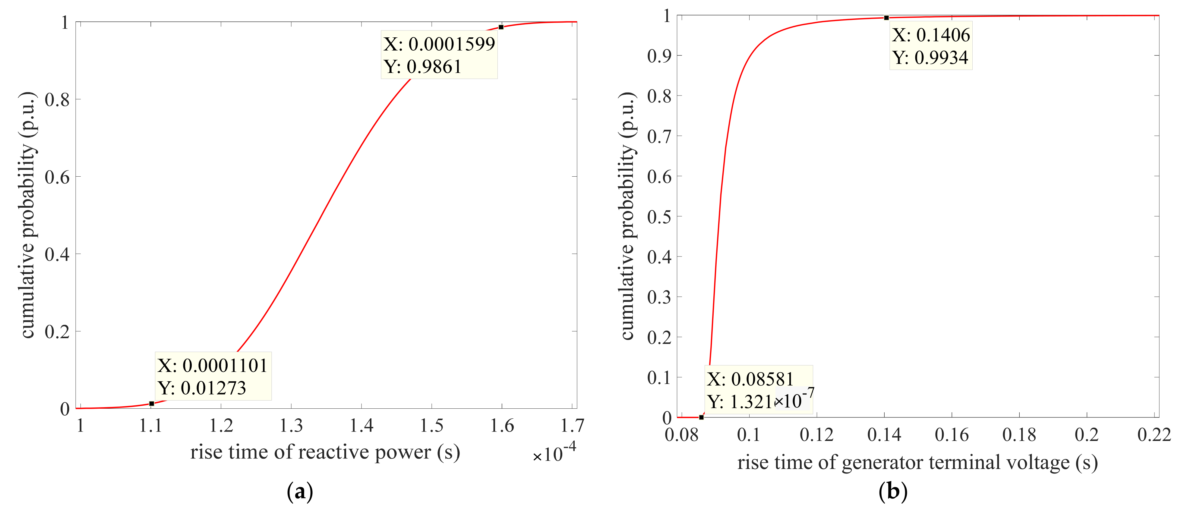
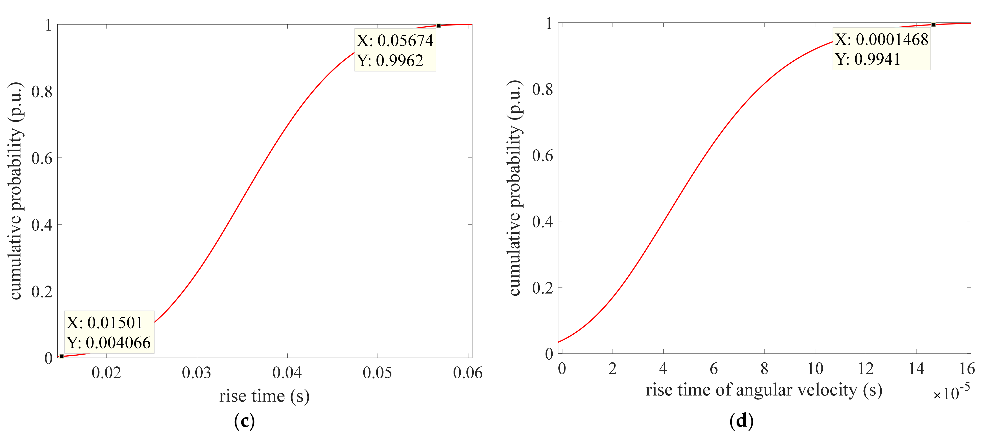
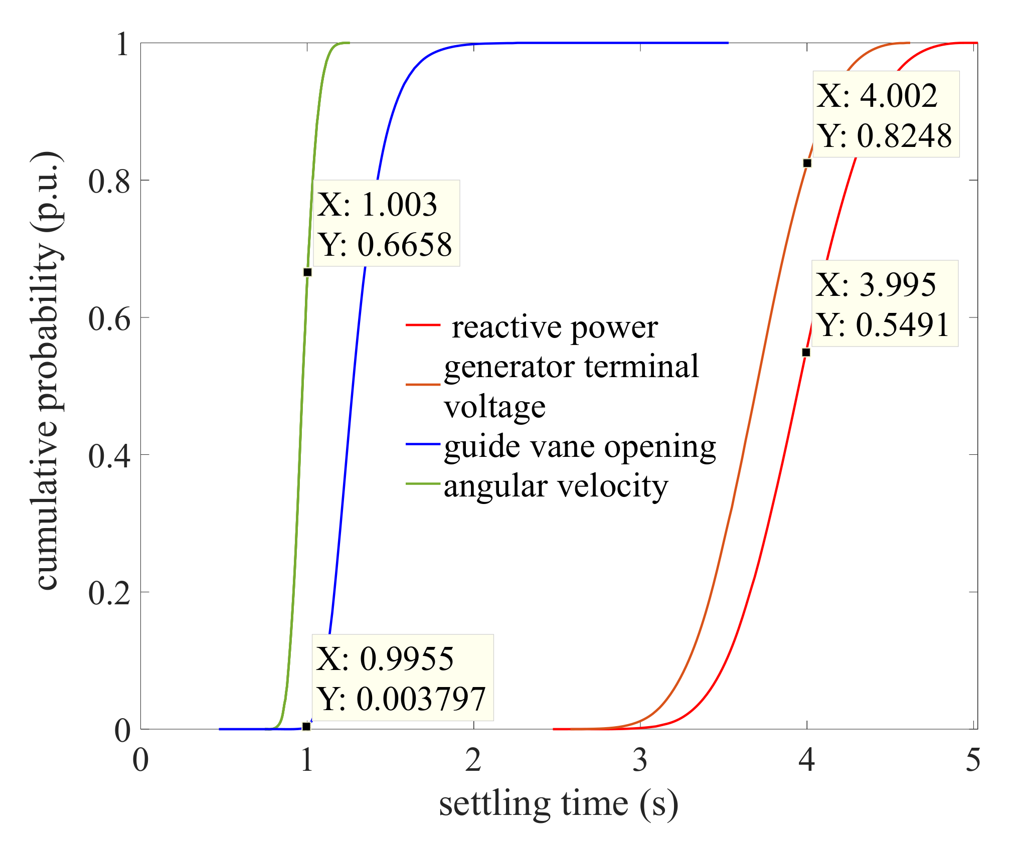
For the same DPI, the cumulative probability distributions of different output variables are significantly different from each other. Regarding different DPIs, the cumulative probability distributions of the same output variable are also different. In general, the settling time is larger than rising time.
(3)
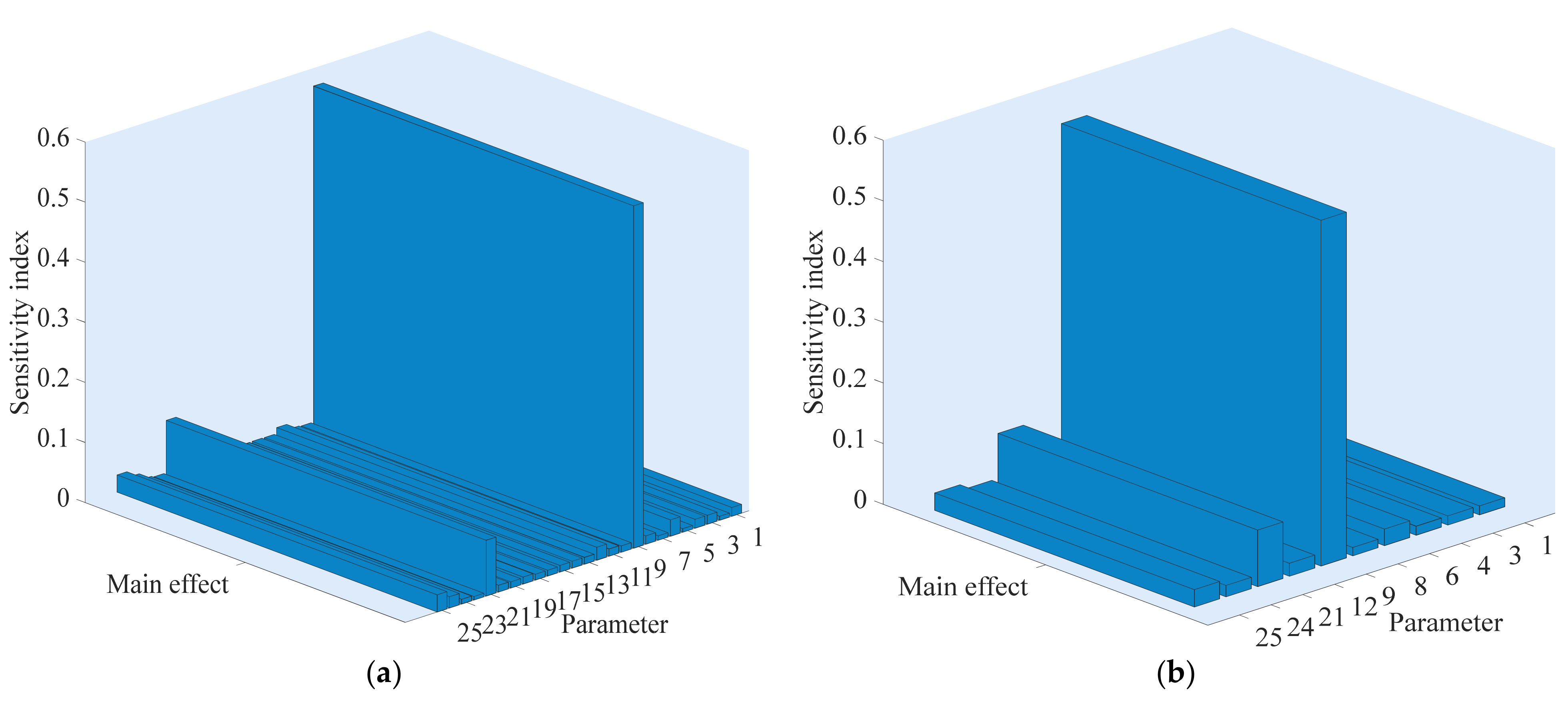
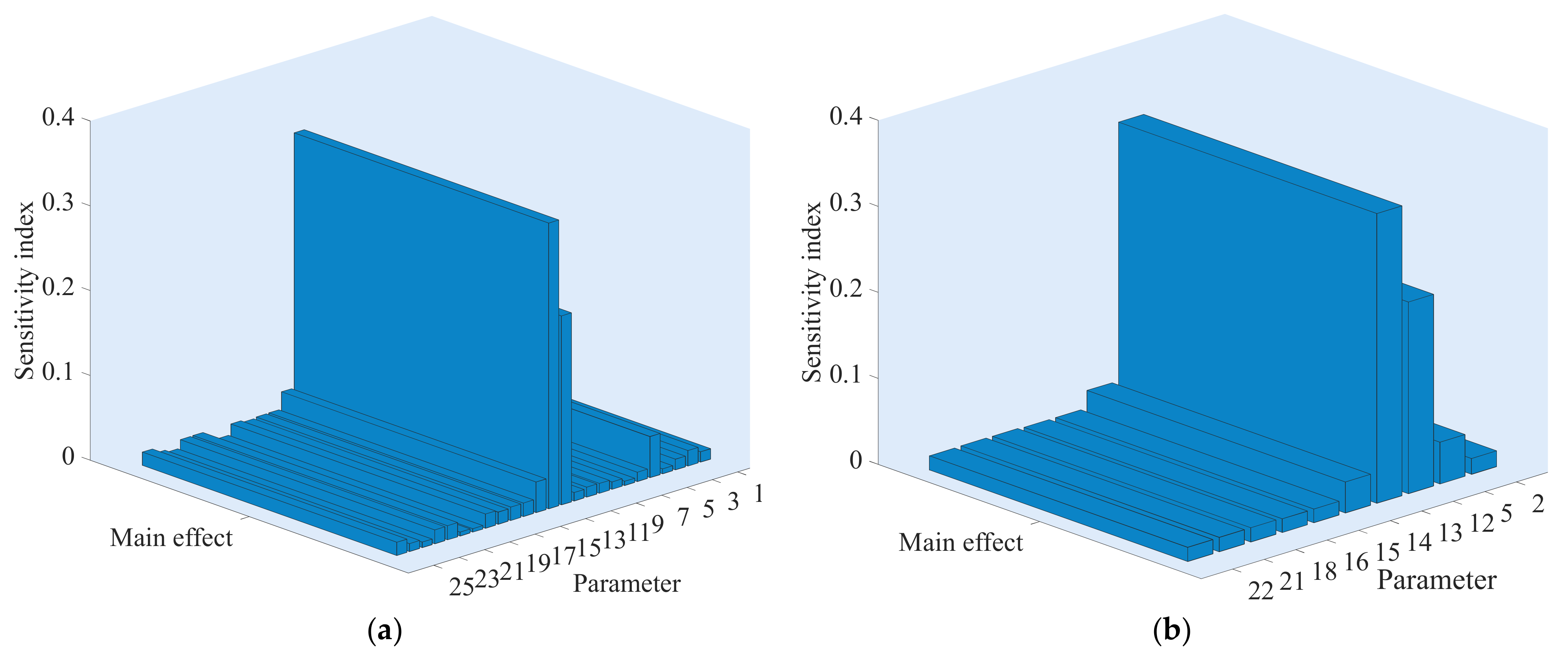
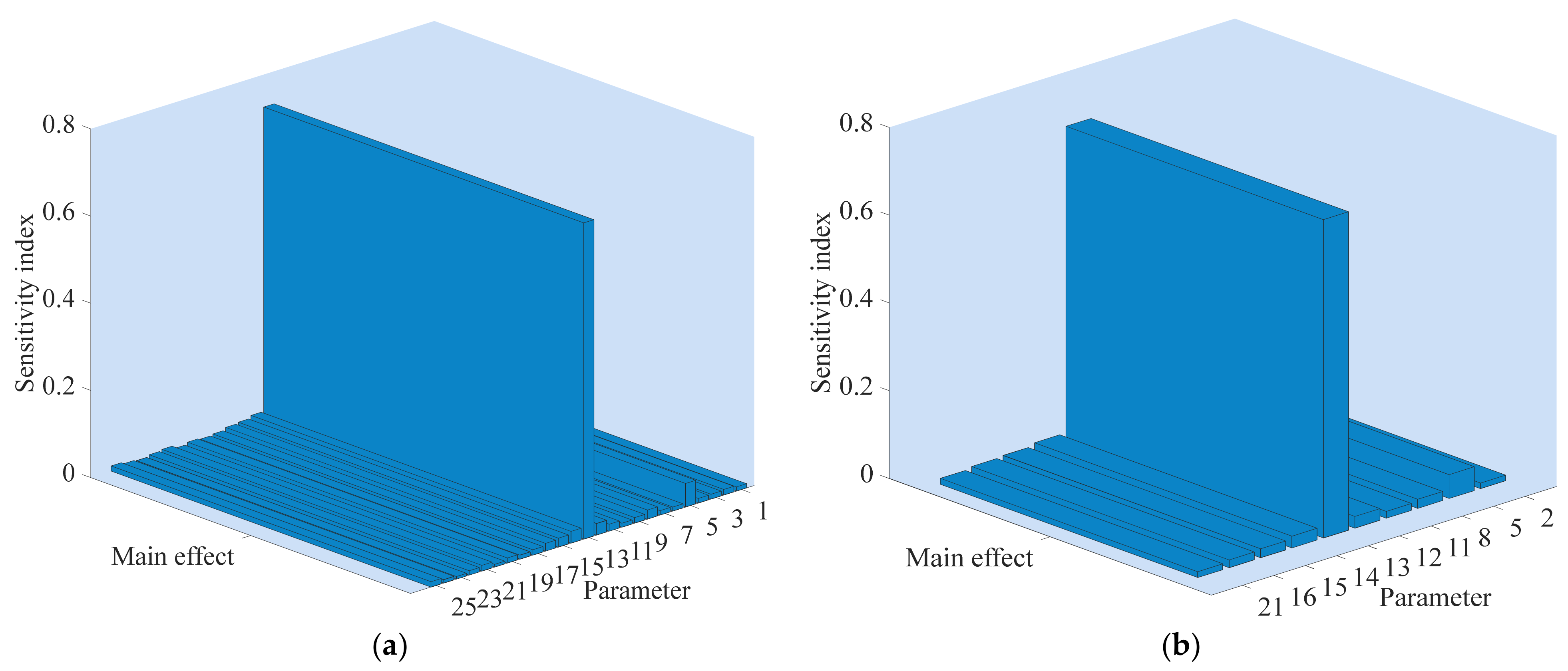
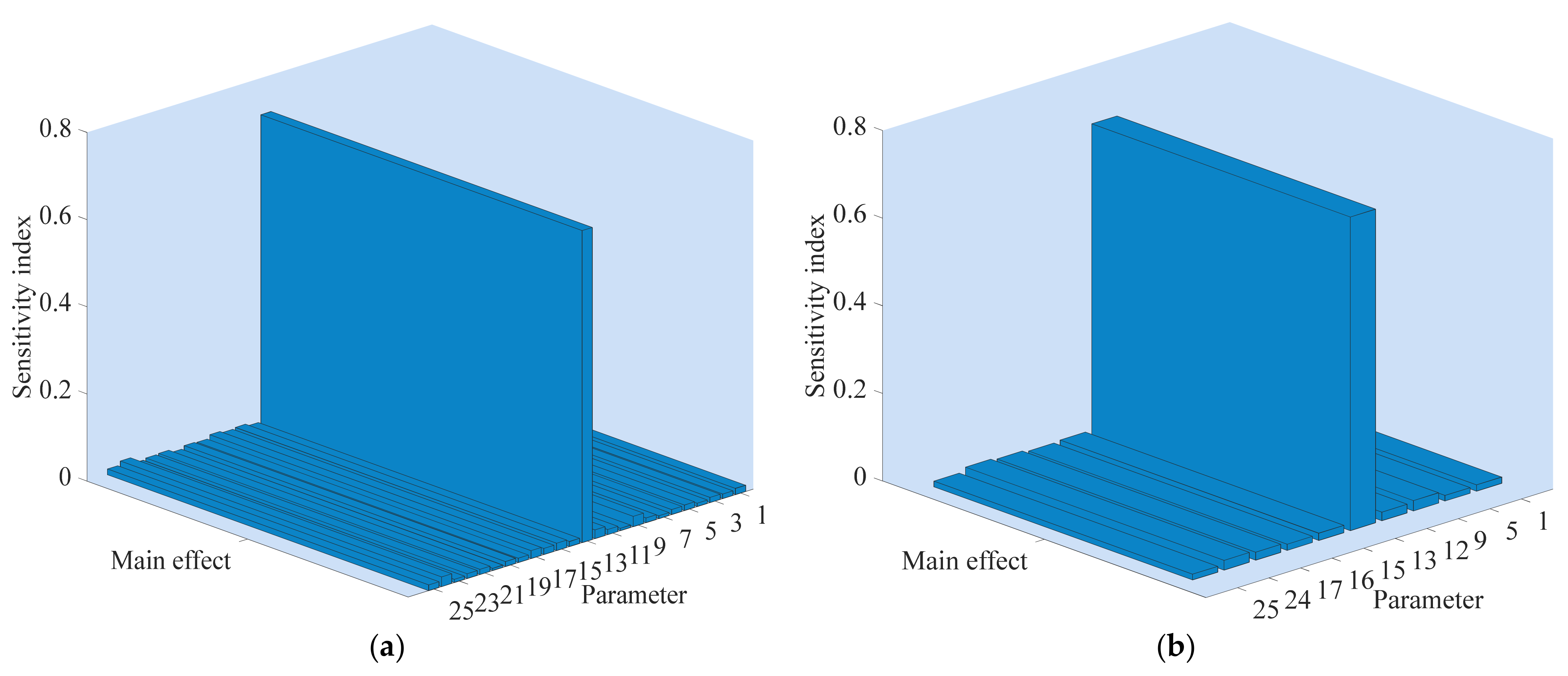
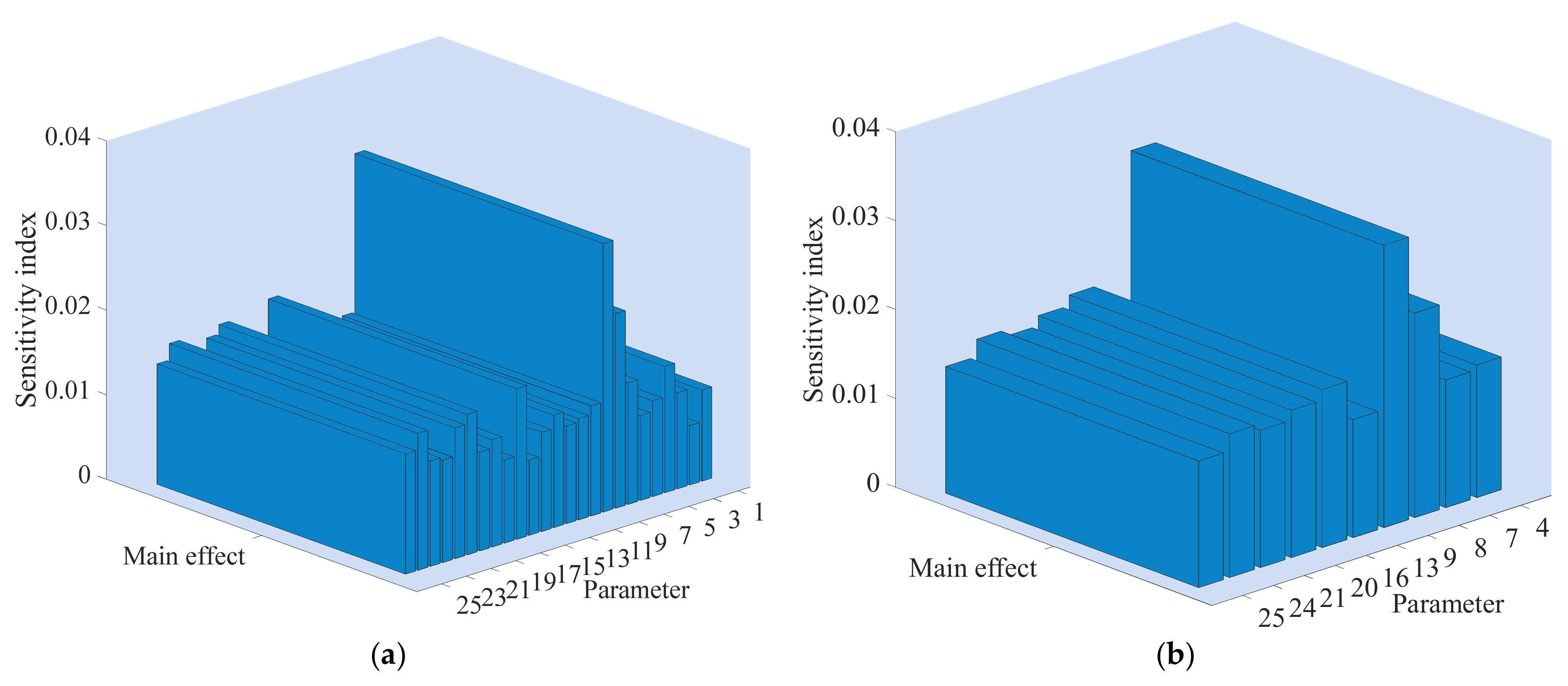
The sensitivity degree of different DPIs to system parameters is obviously different, and even the same parameter has a different effect on the response speed and response stability of the angular velocity. The total contribution rate of the top 10 sensitive parameters on the rise time, settling time, peak value, peak time and overshoot of the angular velocity is 81.77%, 74.45%, 72.55%, 87.15% and 17.764%, respectively. Meanwhile, parameters of WPGS and PPGS have the ability to indirectly affect the angular velocity of PSPP by interacting with other parameters.
(4)
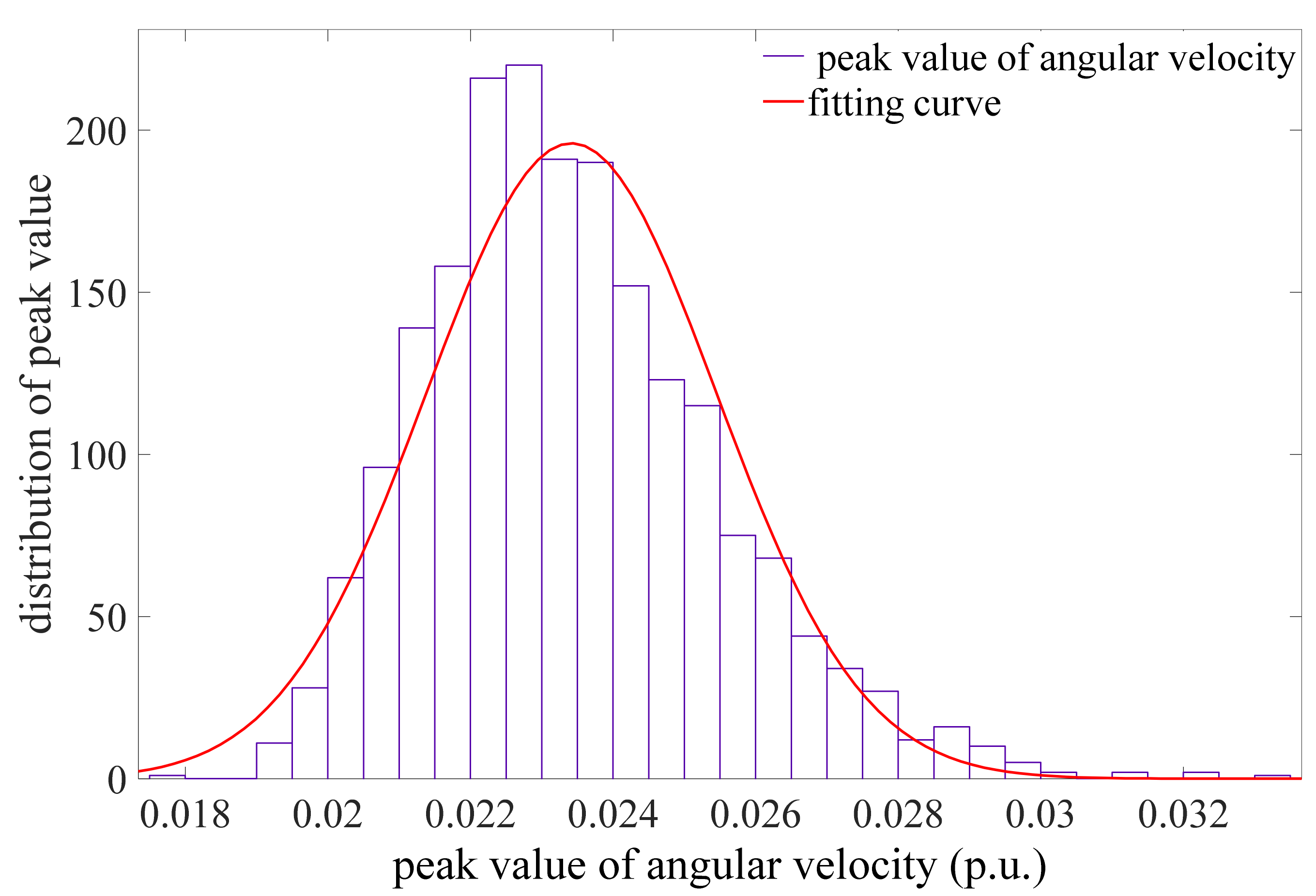
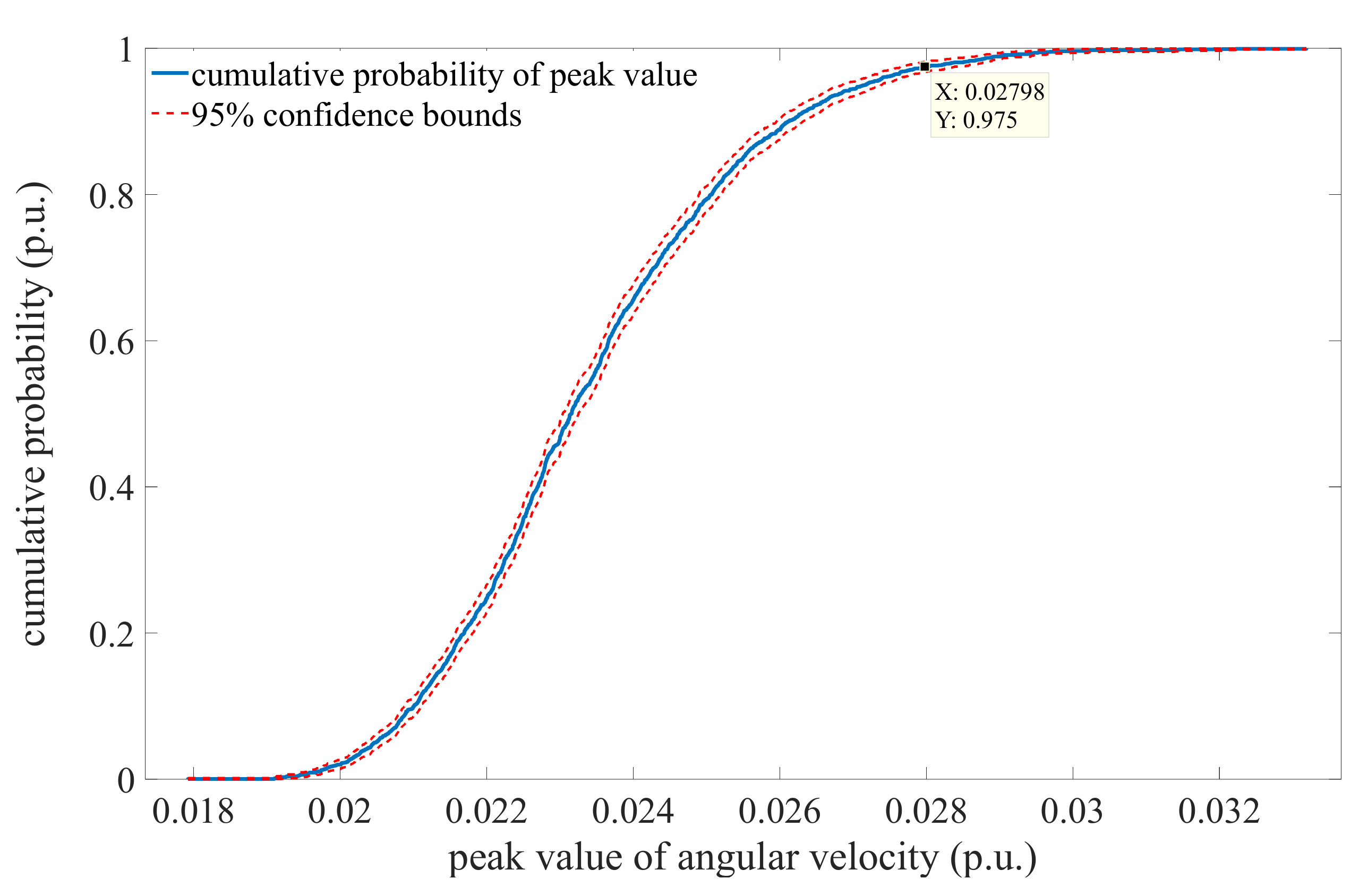
The peak value of angular velocity is distributed between 0.017 and 0.034. Most of the peak value of the angular velocity is in the range of 0.022 to 0.024, and the values on both sides are relatively small. There is a 2.5% probability that the system cannot meet the requirements of operation reliability, which may have a bad impact on the corresponding equipment or even threaten the normal operation of the system.
This paper takes parameters uncertainty into account to investigate the regulation characteristics of PSPP in a WSH hybrid power system. Only reactive power, generator terminal voltage, guide vane opening and angular velocity are considered as the research objects. In the future work, similar studies can be conducted to investigate the influence of parameters on other output variables associated with the wind, solar or hydro subsystem.

Author Contributions

Conceptualization, B.X. and J.Z. (Jingjing Zhang); methodology, B.X.; software, B.X.; validation, B.X. and M.E.; formal analysis, B.X. and J.Z. (Jingjing Zhang); investigation, M.E. and E.E.; resources, D.C.; data curation, D.C.; writing—original draft preparation, B.X. and J.Z. (Jingjing Zhang); writing—review and editing, B.X., J.Z. (Jingjing Zhang) and J.Z. (Junzhi Zhang); visualization, M.E. and E.E.; supervision, D.C.; project administration, D.C.; funding acquisition, B.X. All authors have read and agreed to the published version of the manuscript.

Funding

This research was funded by Beibei Xu of the Chinese Universities Scientific Fund, grant number 2452020210; Beibei Xu of the Open Research Fund Program of State Key Laboratory of Eco-hydraulics in the Northwest Arid Region, Xi’an University of Technology, grant number K4020121034; Beibei Xu of the Postdoctoral fund of Powerchina Northwest Engineering Corporation Limited, grant number kjb2021xz05. The APC was funded by Postdoctoral fund of Powerchina Northwest Engineering Corporation Limited, grant number kjb2021xz05.

Acknowledgments

This work was supported by the Chinese Universities Scientific Fund (Grant No. 2452020210); Open Research Fund Program of State Key Laboratory of Eco-hydraulics in the Northwest Arid Region, Xi’an University of Technology, (Grant No. K4020121034); Postdoctoral fund of Powerchina Northwest Engineering Corporation Limited (Grant No. kjb2021xz05).

Conflicts of Interest

The authors declare no conflict of interest.

Appendix A

Table A1. Dynamic performance indexes of system under unit step response.
Dynamic Performance Indexes of System under Unit Step Response
Water 13 02548 i001
DPIsEquationsSymbol and physical meaning
tr t r = π arctan 1 ξ 2 ξ ω d ξ: the damping ratio
ωd: the damped oscillation frequency, ωd = ωn(1 − ξ2)1/2
ts t s = 4 ξ ω n , Δ = 2 % 3 ξ ω n , Δ = 5 % ωn: the underdamped oscillation frequency
Δ: the error band
tp t p = π ω d ωd: the damped oscillation frequency, ωd= ωn(1−ξ2)1/2
os o s = e ξ π 1 ξ 2 × 100 % ξ: the damping ratio
p------------

Appendix B

Table A2. The basic characteristics of the parameters of the WSH hybrid system.
No.ParameterPhysical MeaningUnitMeanVarianceDistribution
1Ttransfer function parameterp.u.101Normal
2Kpproportional adjustment coefficientp.u.1.60.16Normal
3bpadjustment coefficientp.u.0.010.001Normal
4Kddifferential adjustment coefficients20.2Normal
5Atturbine gainp.u.1.15340.11534Normal
6Dtdamping factorp.u.50.5Normal
7fphead loss coefficientsp.u.0.00280.00028Normal
8qnlno-load flow deviationp.u.0.150.015Normal
9T0transfer function parameterp.u.0.470.047Normal
10Td0transient time constant of d-axis in short circuitp.u.1.010.101Normal
11Td00super transient time constant of d-axis in short circuitp.u.0.0450.0045Normal
12Tq00super transient time constant of q-axis in short circuitp.u.0.0450.0045Normal
13Hinertia coefficientp.u.1.50.15Normal
14Ffriction factorp.u.0.280.028Normal
15Karegulator gainp.u.6.50.65Normal
16Rsstator resistancep.u.0.0230.0023Normal
17Llsstator inductancep.u.0.180.018Normal
18Rrrotor resistancep.u.0.0160.0016Normal
19Llrrotor inductancep.u.0.160.016Normal
20Lmmagnetizing inductancep.u.2.90.29Normal
21H1wind inertia constantp.u.0.6850.0685Normal
22F1wind friction factorp.u.0.210.021Normal
23WSwind speedm/s202Normal
24Ncellm12number of photorefractive array unitsp.u.969.6Normal
25Irintensity of illuminationw/m21500150Normal

References

  1. Rosa, C.D.C.S.; Costa, K.A.; Christo, E.D.; Bertahone, P.B. Complementarity of hydro, photovoltaic, and wind power in Rio de Janeiro state. Sustainability 2017, 9, 1130. [Google Scholar]
  2. Hou, J.J.; Li, C.S.; Guo, W.C.; Fu, W.L. Optimal successive start-up strategy of two hydraulic coupling pumped storage units based on multi-objective control. Int. J. Electr. Power Energy Syst. 2019, 111, 398–410. [Google Scholar] [CrossRef]
  3. Yang, W.J.; Yang, J.D. Advantage of variable-speed pumped storage plants for mitigating wind power variations: Integrated modelling and performance assessment. Appl. Energy 2019, 237, 720–732. [Google Scholar] [CrossRef]
  4. Sarasua, J.I.; Perez-Diaz, J.I.; Wilhelmi, J.R.; Sanchez-Fernandez, J.A. Dynamic response and governor tuning of a long penstock pumped-storage hydropower plant equipped with a pump-turbine and a doubly fed induction generator. Energy Convers. Manag. 2015, 106, 151–164. [Google Scholar] [CrossRef]
  5. Xu, B.B.; Chen, D.Y.; Venkateshkumar, M.; Xiao, Y.; Yue, Y.; Xing, Y.Q.; Li, P.Q. Modeling a pumped storage hydropower integrated to a hybrid power system with solar-wind power and its stability analysis. Appl. Energy 2019, 248, 446–462. [Google Scholar] [CrossRef]
  6. Han, S.; Zhang, L.N.; Liu, Y.Q.; Zhang, H.; Yan, J.; Li, L.; Lei, X.H.; Wang, X. Quantitative evaluation method for the complementarity of wind-solar-hydro power and optimization of wind-solar ratio. Appl. Energy 2019, 236, 973–984. [Google Scholar] [CrossRef]
  7. François, B.; Hingray, B.; Raynaud, D.; Borga, M.; Creutin, J.D. Increasing climate-related-energy penetration by integrating run-of-the river hydropower to wind/solar mix. Renew. Energy 2016, 87, 686–696. [Google Scholar] [CrossRef]
  8. Cantao, M.P.; Bessa, M.R.; Bettega, R.; Detzel, D.H.M.; Lima, J.M. Evaluation of hydro-wind complementarity in the Brazilian territory by means of correlation maps. Renew. Energy 2017, 101, 1215–1225. [Google Scholar] [CrossRef]
  9. Tang, R.B.; Yang, J.D.; Yang, W.J.; Zou, J.; Lai, X. Dynamic regulation characteristics of pumped-storage plants with two generating units sharing common conduits and busbar for balancing variable renewable energy. Renew. Energy 2019, 135, 1064–1077. [Google Scholar] [CrossRef]
  10. Martinez-Lucas, G.; Sarasua, J.I.; Sanchez-Fernandez, J.A.; Wilhelmi, J.R. Power-frequency control of hydropower plants with long penstocks in isolated systems with wind generation. Renew. Energy 2015, 83, 245–255. [Google Scholar] [CrossRef] [Green Version]
  11. Martinez-Lucas, G.; Sarasua, J.I.; Sanchez-Fernandez, J.A.; Wilhelmi, J.R. Frequency control support of a wind-solar isolated system by a hydropower plant with long tail-race tunnel. Renew. Energy 2016, 90, 362–376. [Google Scholar] [CrossRef] [Green Version]
  12. Parida, A.; Chatterjee, D. An improved control scheme for grid connected doubly fed induction generator considering wind-solar hybrid system. Int. J. Electr. Power Energy Syst. 2016, 77, 112–122. [Google Scholar] [CrossRef]
  13. Qin, Z.L.; Li, W.Y.; Xiong, X.F. Incorporating multiple correlations among wind speeds, photovoltaic powers and bus loads in composite system reliability evaluation. Appl. Energy 2013, 110, 285–294. [Google Scholar] [CrossRef]
  14. Hu, P.; Karki, R.; Billinton, R. Reliability evaluation of generating systems containing wind power and energy storage. IET Gener. Transm. Distrib. 2009, 3, 783–791. [Google Scholar] [CrossRef]
  15. Zheng, Y.N.; Ren, D.M.; Guo, Z.Y.; Hu, Z.G.; Wen, Q. Research on integrated resource strategic planning based on complex uncertainty simulation with case study of China. Energy 2019, 180, 772–786. [Google Scholar] [CrossRef]
  16. Billinton, R.; Karki, R. Incorporating wind power in generating system reliability evaluation. Int. J. Syst. Assur. Eng. Manag. 2010, 1, 120–128. [Google Scholar] [CrossRef]
  17. Hashemi-Dezaki, H.; Askarian-Abyaneh, H.; Haeri-Khiavi, H. Impacts of direct cyber-power interdependencies on smart grid reliability under various penetration levels of microturbine/wind/solar distributed generations. IET Gener. Transm. Distrib. 2016, 10, 928–937. [Google Scholar] [CrossRef]
  18. Li, H.H.; Mahmud, M.A.; Arzaghi, E.; Abbassi, R.; Chen, D.Y.; Xu, B.B. Assessments of economic benefits for hydro-wind power systems: Development of advanced model and quantitative method for reducing the power wastage. J. Clean Prod. 2020, 277, 123823. [Google Scholar] [CrossRef]
  19. Ma, T.; Yang, H.; Lu, L.; Peng, J. Technical feasibility study on a standalone hybrid solar-wind system with pumped hydro storage for a remote island in Hong Kong. Renew. Energy 2014, 69, 7–15. [Google Scholar] [CrossRef]
  20. IEEE Group. Hydraulic turbine and turbine control models for system dynamic studies. IEEE Trans. Power Syst. 1992, 7, 167–179. [Google Scholar] [CrossRef]
  21. Zeng, Y.; Guo, Y.K.; Zhang, L.X.; Xu, T.M.; Dong, H.K. Nonlinear hydro turbine model having a surge tank. Math. Comput. Model. Dyn. Syst. 2013, 19, 12–28. [Google Scholar] [CrossRef] [Green Version]
  22. Wei, S.P. Simulation of Hydraulic Turbine Regulating System, 1st ed.; Huazhong University of Science & Technology Press: Wuhan, China, 2011. (In Chinese) [Google Scholar]
  23. Zhang, H.; Chen, D.Y.; Xu, B.B.; Wang, F.F. Nonlinear modeling and dynamic analysis of hydro-turbine governing system in the process of load rejection transient. Energy Conv. Manag. 2015, 90, 128–137. [Google Scholar] [CrossRef]
  24. Roy, T.K.; Mahmud, M.A.; Oo, A.M.T. Robust adaptive backstepping excitation controller design for higher-order models of synchronous generators in multimachine power systems. IEEE Trans. Power Syst. 2019, 34, 40–51. [Google Scholar] [CrossRef]
  25. Xu, B.B.; Zhang, J.J.; Egusquiza, M.; Chen, D.Y.; Li, F.; Behrens, P.; Egusquiza, E. A review of dynamic models and stability analysis for a hydro-turbine governing system. Renew. Sustain. Energy Rev. 2021, 144, 110880. [Google Scholar] [CrossRef]
  26. Karakasis, N.; Tsioumas, E.; Jabbour, N.; Bazzi, A.M.; Mademlis, C. Optimal efficiency control in a wind system with doubly fed induction generator. IEEE Trans. Power Electron. 2019, 34, 356–368. [Google Scholar] [CrossRef]
  27. Coral-Enriquez, H.; Cortes-Romero, J.; Dorado-Rojas, S.A. Rejection of varying-frequency periodic load disturbances in wind-turbines through active disturbance rejection-based control. Renew. Energy 2019, 141, 217–235. [Google Scholar] [CrossRef]
  28. Bedoud, K.; Rhif, A.; Bahi, T.; Merabet, H. Study of a double fed induction generator using matrix converter: Case of wind energy conversion system. Int. J. Hydrog. Energy 2018, 43, 11432–11441. [Google Scholar] [CrossRef]
  29. Ranjbaran, P.; Yousefi, H.; Gharehpetian, G.B.; Astaraei, F.R. A review on floating photovoltaic (FPV) power generation units. Renew. Sustain. Energy Rev. 2019, 110, 332–347. [Google Scholar] [CrossRef]
  30. Ram, J.P.; Babu, T.S.; Rajasekar, N. A comprehensive review on solar PV maximum power point tracking techniques. Renew. Sustain. Energy Rev. 2017, 67, 826–847. [Google Scholar] [CrossRef]
  31. Kumari, P.A.; Geethanjali, P. Parameter estimation for photovoltaic system under normal and partial shading conditions: A survey. Renew. Sustain. Energy Rev. 2018, 84, 1–11. [Google Scholar] [CrossRef]
  32. Patelli, E.; Pradlwarter, H.J.; Schueller, G.I. Global sensitivity of structural variability by random sampling. Comput. Phys. Commun. 2010, 181, 2072–2081. [Google Scholar] [CrossRef] [Green Version]
  33. Pradlwarter, H.J. Relative importance of uncertain structural parameters, part I: Algorithm. Comput. Mech. 2007, 40, 627–635. [Google Scholar] [CrossRef]
  34. Iooss, B.; Le Gratiet, L. Uncertainty and sensitivity analysis of functional risk curves based on Gaussian processes. Reliab. Eng. Syst. Saf. 2019, 187, 58–66. [Google Scholar] [CrossRef] [Green Version]
  35. Saltelli, A.; Chan, K.; Scott, E.M. Sensitivity Analysis; Wiley Series in Probability and Statistics; Wiley: New York, NY, USA, 2000. [Google Scholar]
  36. Sudret, B. Global sensitivity analysis using polynomial chaos expansions. Reliab. Eng. Syst. Saf. 2008, 93, 964–979. [Google Scholar] [CrossRef]
  37. Klepper, O. Multivariate aspects of model uncertainty analysis: Tools for sensitivity analysis and calibration. Ecol. Model. 1997, 101, 1–13. [Google Scholar] [CrossRef]
  38. Iooss, B.; Lemaitre, P. A review on global sensitivity analysis methods. Oper. Res. Comput. Sci. Interfaces 2015, 59, 101–122. [Google Scholar]
  39. Xu, B.B.; Chen, D.Y.; Zhang, X.L.; Alireza, R. Parametric uncertainty in affecting transient characteristics of multi-parallel hydropower systems in the successive load rejection. Int. J. Electr. Power Energy Syst. 2019, 106, 444–454. [Google Scholar] [CrossRef]
  40. Xu, B.B.; Chen, D.Y.; Patelli, E.; Shen, H.J.; Park, J.H. Mathematical model and parametric uncertainty analysis of a hydraulic generating system. Renew. Energy 2019, 136, 1217–1230. [Google Scholar] [CrossRef] [Green Version]
  41. Cai, G.Q.; Elishakoff, I. Refined second-order reliability analysis. Struct. Saf. 1994, 14, 267–276. [Google Scholar] [CrossRef]
  42. Zhao, H.B.; Ru, Z.L.; Chang, X.; Li, S.J. Reliability analysis using chaotic particle swarm optimization. Qual. Reliab. Eng. Int. 2015, 31, 1537–1552. [Google Scholar] [CrossRef]
  43. Lü, Q.; Sun, H.Y.; Low, B.K. Reliability analysis of ground-support interaction in circular tunnels using the response surface method. Int. J. Rock Mech. Min. Sci. 2011, 48, 1329–1343. [Google Scholar] [CrossRef]
  44. Hasofer, A.M.; Lind, N.C. Exact and invariant second moment code format. J. Eng. Mech. Div. 1974, 100, 111–121. [Google Scholar] [CrossRef]
  45. Low, B.K.; Tang, W.H. Reliability analysis of reinforced embankments on soft ground. Can. Geotech. J. 1997, 34, 672–685. [Google Scholar] [CrossRef]
  46. Low, B.K.; Tang, W.H. Efficient reliability evaluation using spreadsheet. J. Eng. Mech. 1997, 123, 749–752. [Google Scholar] [CrossRef]
Figure 1. A hybrid solar-wind system with pumped storage system.
Water 13 02548 g001
Figure 2. The block diagram of the hydro turbine. At is the hydro-turbine gain. h and q are the deviation of the water head and flow of the hydro turbine, respectively. fp is the head loss coefficient pm is the relative value of the output mechanical power. qn1 is the no-load flow deviation. Δω is the deviation value of the angular velocity of the unit. Dt is the damping factor. hfc is the relative value of the pipe friction head loss. y is the guide vane opening. hq denotes the variation of the water head of the hydro turbine caused by the flow change of the penstock.
Water 13 02548 g002
Figure 3. A typical excitation system configuration. Ut is the generator terminal voltage. Uref is the reference voltage. UR is the output of the voltage regulator. Ef is the excitation voltage. rf is the excitation winding resistance of generator. xad is the inductance coefficient of the d-axis armature reaction. Uf is the output of the excitation system stabilizer. Us is the output of the power system stabilizer. PSS stands for the power system stabilizer.
Water 13 02548 g003
Figure 4. Model of the pumped storage power plant. Vd and Vq are the stator voltage of the d-axis and q-axis, respectively. Pe, Pm and Pref represent the electrical power, the power output of the hydro turbine per unit and the reference output, respectively. Vref, Vstab and Vf are the reference value of the stator terminal voltage, the voltage connected to a power system stabilizer and the field voltage, respectively. A, B and C stand for the stator voltage input/output terminal. a, b and c denote the winding rotor output voltage terminal. dw is the rotor speed deviation.
Water 13 02548 g004
Figure 5. The block diagram of the wind power generation system.
Water 13 02548 g005
Figure 6. The block diagram of the photovoltaic power generation system.
Water 13 02548 g006
Figure 7. The block diagram of the WSH hybrid system.
Water 13 02548 g007
Figure 8. Dynamic characteristics of voltage and current with three−phase short circuit fault of point H occurring as 1.0 s and cleared at 1.04 s. (a) Dynamic characteristics of voltage and current of point W with three−phase short circuit fault of point H occurring at 1.0 s and cleared at 1.04 s. (b) Dynamic characteristics of voltage and current of point S with three−phase short circuit fault of point H occurring at 1.0 s and cleared at 1.04 s. (c) Dynamic characteristics of voltage and current of point W with three−phase short circuit fault of point S occurring at 1.0 s and cleared at 1.04 s. (d) Dynamic characteristics of voltage and current of point S with three−phase short circuit fault of point S occurring at 1.0 s and cleared at 1.04 s.
Water 13 02548 g008
Figure 9. The influence of the wind−solar−hydro system parameters on the DPIs of the reactive power of PSPP. (a) The influence of Ka on the rise time. (b) The influence of Ka on the overshoot. (c) The influence of Td0 on the settling time. (d) The influence of Tq00 and L1s on the peak value and peak time.
Water 13 02548 g009
Figure 10. The influence of the wind−solar−hydro system parameters on the DPIs of the generator terminal voltage of PSPP. (a) The influence of Td0 on the settling time. (b) The influence of Ka on the peak value. (c) The influence of Lm and H1 on the peak value and peak time. (d) The influence of Ncellm12 and Ir on the overshoot.
Water 13 02548 g010
Figure 11. The influence of the wind−solar−hydro system parameters on the DPIs of the guide vane opening of PSPP. (a) The influence of At, F and H on the peak value and peak time. (b) The influence of F on the rise time and settling time. (c) The influence of F on the overshoot.
Water 13 02548 g011
Figure 12. The influence of the wind−solar−hydro system parameters on the DPIs of the angular velocity of PSPP. (a) The influence of H on the settling time. (b) The influence of H on the overshoot.
Water 13 02548 g012
Figure 13. The cumulative probability of the rise time. (a) The cumulative probability of the rise time of the reactive power; (b) The cumulative probability of the rise time of the generator terminal voltage; (c) The cumulative probability of the rise time of the guide vane opening; (d) The cumulative probability of the rise time of the angular velocity.
Water 13 02548 g013aWater 13 02548 g013b
Figure 14. The cumulative probability of the settling time of the reactive power, generator terminal voltage, guide vane opening and angular velocity, respectively.
Water 13 02548 g014
Figure 15. The sensitivity index of parameters of the rise time of the angular velocity. (a) The sensitivity index of 25 parameters; (b) The sensitivity index of the top 10 parameters. The numbers 1 to 25 represent symbols T, Kp, bp, Kd, At, Dt, fp, qnl, T0, Td0, Td00, Tq00, H, F, Ka, Rs, Lls, Rr, Llr, Lm, H1, F1, WS, Ncellm12 and Ir, respectively. For the physical meaning and definitions of these parameters, see Appendix B.
Water 13 02548 g015
Figure 16. The sensitivity index of parameters of the settling time of the angular velocity. (a) The sensitivity index of 25 parameters; (b) The sensitivity index of the top 10 parameters. The numbers 1 to 25 represent symbols T, Kp, bp, Kd, At, Dt, fp, qnl, T0, Td0, Td00, Tq00, H, F, Ka, Rs, Lls, Rr, Llr, Lm, H1, F1, WS, Ncellm12 and Ir, respectively. For the physical meaning and definitions of these parameters, see Appendix B.
Water 13 02548 g016
Figure 17. The sensitivity index of parameters of the peak value of the angular velocity. (a) The sensitivity index of 25 parameters; (b) The sensitivity index of the top 10 parameters. The numbers 1 to 25 represent symbols T, Kp, bp, Kd, At, Dt, fp, qnl, T0, Td0, Td00, Tq00, H, F, Ka, Rs, Lls, Rr, Llr, Lm, H1, F1, WS, Ncellm12 and Ir, respectively. For the physical meaning and definitions of these parameters, see Appendix B.
Water 13 02548 g017
Figure 18. The sensitivity index of parameters of the peak time of the angular velocity. (a) The sensitivity index of 25 parameters; (b) The sensitivity index of the top 10 parameters. The numbers 1 to 25 represent symbols T, Kp, bp, Kd, At, Dt, fp, qnl, T0, Td0, Td00, Tq00, H, F, Ka, Rs, Lls, Rr, Llr, Lm, H1, F1, WS, Ncellm12 and Ir, respectively. For the physical meaning and definitions of these parameters, see Appendix B.
Water 13 02548 g018
Figure 19. The sensitivity index of parameters of the overshoot of the angular velocity. (a) The sensitivity index of 25 parameters; (b) The sensitivity index of the top 10 parameters. The numbers 1 to 25 represent symbols T, Kp, bp, Kd, At, Dt, fp, qnl, T0, Td0, Td00, Tq00, H, F, Ka, Rs, Lls, Rr, Llr, Lm, H1, F1, WS, Ncellm12 and Ir, respectively. For the physical meaning and definitions of these parameters, see Appendix B.
Water 13 02548 g019
Figure 20. Distribution of the peak value of the angular velocity.
Water 13 02548 g020
Figure 21. The cumulative probability of the peak value of the angular velocity.
Water 13 02548 g021
Table 1. The excitation system model of each unit.
UnitEquationParameter
Measure unit G M ( s ) = 1 T r s + 1 Tr: the time constant of the measure unit
s: the Laplace operator
Voltage regulator Water 13 02548 i002Tb, Tc: the time constants used to model equivalent time constants inherent
Ka: the regulator gain
Ta: the regulator time constant
UR: the output of the voltage regulator
Ut: the generator terminal voltage
UR,max, UR,min: the limitation of the voltage
Exciter G E ( s ) = 1 T e s + K e Te: the exciter time constant
Ke: the exciter gain
Excitation system stabilizer G E S S ( s ) = K f 1 + T f s Kf: the gain of the excitation system stabilizer
Tf: the time constant of the excitation system stabilizer
Table 2. Key specifications of the solar panel.
SymbolCharacteristicsValue
Vocthe open circuit voltage64.2 V
Vmpthe optimum operating voltage54.7 V
Iscthe short circuit current5.96 A
Impthe optimum operating current5.58 A
NCellmthe number of photorefractive array units96
betathe temperature coefficient of Voc−0.27269 mV/°C
alphathe temperature coefficient of Isc0.061745 mA/°C
Table 3. The nomenclatures of the wind–solar−hydro hybrid system.
SymbolPhysical MeaningSymbolPhysical Meaning
hqthe relative value of head caused by flowEfdthe exciter output voltage
Hthe inertia coefficientEfthe regulator output
qthe relative value of flowTethe exciter time constant
T0the elastic time of the equivalent penstockKethe exciter gain
αthe water hammer wave speedKathe regulator gain
Lthe length of penstockTathe time constant
Qrthe rated flowKfthe gain of the excitation system stabilizer
Hrthe rated headTfthe time constant of the excitation system stabilizer
Aithe section dimension of penstockTb, Tcthe time constants used to model equivalent time constants inherent
gthe acceleration of gravityVt0the initial values of the terminal voltage
sthe Laplace operatorVf0the initial values of the field voltage
Tythe engager relay time constanttrthe low-pass filter time constant
Kpthe proportional adjustment coefficientPethe electrical power
Kithe integral adjustment coefficientPrefthe reference output
Kdthe differential adjustment coefficientA, B, Cthe stator voltage input/output terminal
δthe relative value of the rotor anglea, b, cthe winding rotor output voltage terminal
ωthe relative value of the generator rotor speeddwthe rotor speed deviation
ythe relative value of the guide vane openingQthe output reactive power
Pmthe power output of the hydro turbine per unitδthe power angle
Atthe gain coefficient of the turbineifdthe field current
qn1the no-loading flow per unittrthe rise time
Dtthe mechanical damping coefficient of the turbinetsthe settling time
Δωthe difference of the angular velocitypthe peak value
hfcthe relative value of the pipe friction head losstpthe peak time
Kathe regulator gainosthe overshoot
Vrefthe reference value of the stator terminal voltageTthe transfer function parameter
Vdthe stator voltage of the d-axisVqthe stator voltage of q-axis
Vtfthe stator terminal voltageF1the wind friction factor
Rsthe stator resistanceH1the wind inertia constant
Llrthe rotor inductanceLmthe magnetizing inductance
WSthe wind speedNcellm12the number of photorefractive array units
Irthe intensity of illuminationPLthe load power
Xlthe positive sequence reactanceXdthe d-axis synchronous reactance
Xd0the d-axis transient reactanceXd00the d-axis super-transient reactance
Xq00the q-axis super-transient reactanceXqthe q-axis synchronous reactance
Rs1the stator resistancexthe possible value of the uncertain component
Vfthe field voltageVstabthe voltage connected to the power system stabilizer
Z0the surge impedance per unit of the equivalent penstockTd0the transient time constant of the straight axis in short circuit
Tq00the super transient time constant of the quadrature axis in short circuitTd00the super transient time constant of the straight axis in short circuit
Sthe state domainF’the failure domain
μthe vector of mean valuesμiNthe equivalent normal mean
Fthe friction factorCthe covariance matrix
[R]the correlation matrixβthe Hasofer–Lind index
αthe directional vector at the design point in U-spaceBthe scaled second-order derivatives of g ˜ ( u ) at u*
φ(β)the cumulative distribution function of the standard normal variablePfthe probability of failure
Xthe vector representing the set of random variables xiσiNthe equivalent normal standard deviation of random variable xi
Utthe generator terminal voltageURthe output of the voltage regulator
Urefthe reference voltageEfthe excitation voltage
xadthe inductance coefficient of d-axis armature reactionrfthe excitation winding resistance of the generator
Usthe output of the power system stabilizerUfthe output of the excitation system stabilizer
Trthe time constant of the measure unitLthe inductance
ψthe magnetic fluxLmthe mutual inductance
TLthe resistance torque of loadJthe rotational inertia
pnthe pole pairsus, is, Rsthe voltage, current, resistance of stator
PWTthe power output of the wind turbinePratedthe rated electrical power of the wind turbine
vci, vcothe cut-in and cut-off wind speedvrthe rated wind speed
Iphthe photo currentI0the diode saturation current
Rsthe series resistanceRpthe shunt/parallel resistance
Vtthe diode thermal voltagePA, IA, VAthe power output, current, and voltage of the PV array
Table 4. The statistics of dynamic performance indexes of the reactive power and generator terminal voltage.
Simulation No.Ke (p.u.)Ki (s−1)Reactive PowerGenerator Terminal Voltage
tr (s)ts (s)p (p.u.)tp (s)tr (s)ts (s)p (p.u.)tp (s)Os (p.u.)
160.550.000290.708357.504720.00630.058930.59551226.5880.244751.405
270.550.000170.837747.504820.00630.048691.15137226.260.244751.99228
370.550.000170.837747.504820.00630.048691.15137226.260.244751.99228
470.550.000170.837747.504820.00630.048691.15137226.260.244751.99228
570.10.000160.838477.504820.00630.048691.15186226.2610.244751.99339
6610.000290.708337.504720.00630.058920.59554226.5880.244751.40557
770.550.000170.837747.504820.00630.048691.15137226.260.244751.99228
870.550.000170.837747.504820.00630.048691.15137226.260.244751.99228
9710.000160.838627.504820.00630.048691.1528226.260.244751.99509
1070.550.000170.837747.504820.00630.048691.15137226.260.244751.99228
1170.550.000170.837747.504820.00630.048691.15137226.260.244751.99228
12810.000071.397287.504890.00630.047161.9153226.0130.244752.47662
1380.550.000071.397127.504890.00630.047161.91419226.0140.244752.47599
1480.10.000071.377547.504890.00630.047171.9127226.0140.244752.47537
1570.550.000170.837747.504820.00630.048691.15137226.260.244751.99228
1660.10.000290.708357.504720.00630.058930.5955226.5880.244751.40489
The bar in each cell indicates the relative magnitude of the values with the same color. Ke and Ki are the exciting gain and the integral adjustment coefficient, respectively. tr, ts, p, tp and Os are the rise time, settling time, peak value, peak time and overshoot, respectively.
Table 5. The dynamic performance indexes of the guide vane opening and angular velocity.
Simulation No.Ke (p.u.)Ki (s−1)Guide Vane OpeningAngular Velocity
tr (s)ts (s)p (p.u.)tp (s)Os (p.u.)tr (s) ×10−5ts (s)p (p.u.)tp (s)Os (p.u.)
160.550.018371.156210.218950.22785188.5073.991.101651.051180.2485.1204
270.550.018531.164950.217930.22795185.1653.320.985611.050780.24855.0801
370.550.018531.164950.217930.22795185.1653.320.985611.050780.24855.0801
470.550.018531.164950.217930.22795185.1653.320.985611.050780.24855.0801
570.10.018431.164830.21750.22795187.6363.410.985631.050770.24855.07975
6610.018551.156570.219670.2279184.3263.951.101561.051180.2485.12074
770.550.018531.164950.217930.22795185.1653.320.985611.050780.24855.0801
870.550.018531.164950.217930.22795185.1653.320.985611.050780.24855.0801
9710.018631.165060.218360.24795182.753.280.985591.050780.24855.08045
1070.550.018531.164950.217930.22795185.1653.320.985611.050780.24855.0801
1170.550.018531.164950.217930.22795185.1653.320.985611.050780.24855.0801
12810.01871.179190.217360.228181.573.280.985591.050470.24855.0493
1380.550.018591.179130.216930.228183.922.910.991591.050470.24855.0493
1480.10.018491.179060.21650.228186.3212.930.991591.050470.24855.04902
1570.550.018531.164950.217930.22795185.1653.320.985611.050780.24855.0801
1660.10.018341.156130.218810.22785189.3624.001.101661.051180.2485.12006
The bar in each cell indicates the relative magnitude of the values with the same color. Ke and Ki are the exciting gain and the integral adjustment coefficient, respectively. tr, ts, p, tp and Os are the rise time, settling time, peak value, peak time and overshoot, respectively.
Table 6. Sensitivity index results of DPIs of angular velocity.
Rise Time (tr)Settling Time (ts) Peak Value (p)
No.ParameterSensitivity IndexRankingNo.ParameterSensitivity IndexRankingNo.ParameterSensitivity IndexRanking
1T1.48%92Kp1.83%52Kp1.29%10
3bp1.51%75At4.85%35At5.44%2
4Kd1.51%812Tq0022.29%28qnl2.07%5
6Dt2.72%413H33.70%111Td001.58%8
8qnl1.39%1014F3.62%412Tq002.66%4
9T056.99%115Ka1.60%913H72.55%1
12Tq002.14%516Rs1.58%1014F2.69%3
21H19.30%218Rr1.67%715Ka2.05%6
24Ncellm121.88%621H11.67%616Rs1.78%7
25Ir2.86%322F11.65%821H11.33%9
Total--81.77%--Total--74.45%--Total--93.45%--
Peak time (pt)Overshoot (Os)Note
No.ParameterSensitivity indexRankingNo.ParameterSensitivity indexRankingColour in cells: gradient change from green through yellow to red represents sensitivity from good to bad.
1T1.44%74Kd1.49%7
5At1.28%107fp1.44%8
9T02.36%28qnl2.30%2Theses sensitivity indexes values of dynamic performance indexes are based on angular velocity.
12Tq001.99%49T03.18%1
13H71.59%113H1.33%10
15Ka1.68%616Rs1.78%3
16Rs1.42%820Lm1.66%4Physical meaning and definitions of these parameters see Table 3.
17Lls1.84%521H11.55%6
24Ncellm122.23%324Ncellm121.62%5The longer the blue data bar, the weaker the sensitivity of the parameter.
25Ir1.32%925Ir1.42%9
Total--87.15%--Total--17.76%--
Publisher’s Note: MDPI stays neutral with regard to jurisdictional claims in published maps and institutional affiliations.

