Evaluation of Vegetation Indices and Phenological Metrics Using Time-Series MODIS Data for Monitoring Vegetation Change in Punjab, Pakistan

Abstract

In arid and semi-arid regions, it is essential to monitor the spatiotemporal variability and dynamics of vegetation. Among other provinces of Pakistan, Punjab has produced a significant number of crops. Recently, Punjab, Pakistan, has been described as a global hotspot for extremes of climate change. In this study, the soil adjusted vegetation index (SAVI), normalized vegetation difference index (NDVI), and enhanced vegetation index (EVI) were comprehensively evaluated to monitor vegetation change in Punjab, Pakistan. The time-series MODIS (Moderate Resolution Imaging Spectroradiometer) data of different periods were used. The mean annual variability of the above vegetation indices (VIs) from 2000 to 2019 was evaluated and analyzed. For each type of vegetation, two phenological metrics (i.e., for the start of the season and end of the season) were calculated and compared. The spatio-temporal image analysis of the mean annual vegetation indices revealed similar patterns and varying vegetation conditions. In the forests and vegetation areas with sparse vegetation, the EVI showed high uncertainty. The phenological metrics of all vegetation indices were consistent for most types of vegetation. However, the NDVI result had the greatest variance between the start and end of season. The lowest annual VI variability was mainly observed in the southern part of the study area (less than 10% of the study area) based on the statistical analysis of spatial variability. The mean annual spatial variability of NDVI was <20%, SAVI was 30%, and EVI ranged between 10–20%. More than 40% of the variability was observed in the NDVI and SAVI vegetation indices.

1. Introduction

Semi-arid regions cover about 15% of the Earth’s land surface and the spatial and temporal patterns of rainfall in these regions are very variable, which causes drastic vari-ability in the spatiotemporal distribution, production, and development of vegetation [1,2]. Over recent decades, many semi-arid and dryland habitats have faced greater pressures from human-induced activities and climate change [3,4,5]. To better understand climatic change and anthropogenic impacts on dryland and semi-arid ecosystems, information on the vegetation’s spatiotemporal variability is the key source. Satellite-based knowledge is an important tool in tracking vegetation variability and dynamics, with the potential for broad spatial coverage and regular explanations [6,7]. The dataset of the spectral vegetation index is particularly well-related to the leaf area index (LAI), the abundance of chlorophyll, the absorption of gross-primary-production (GPP), and photosynthetically active radiation (PAR) [8,9,10]. To monitor semi-arid and dryland vegetation activity and spot changes in growth and phenology of vegetation [11,12,13], vegetation indices time-series have often been used [14,15,16,17].

The polar-orbiting MODIS (Moderate Resolution Imaging Spectroradiometer) sensor allows for the monitoring and measurement of vegetation and environmental indices. MODIS-derived data have a superior spatial and radiometric resolution than that of the Advanced Very High-Resolution Radiometer (AVHRR) sensor and thus provides an enhanced radiometric, spatial, and spectral representation of surface vegetation conditions [18,19]. Among the generally used datasets in the monitoring of vegetation dynamics, the normalized vegetation difference index (NDVI) time-series is noteworthy. Nevertheless, the NDVI has some restrictions relating to soil reflectance, affecting the index and contributing to different index values for various conditions of soil and moisture being observed for similar biophysical properties of the canopy [20]. A variable of soil adjustment ‘L’ was proposed to interpret the nonlinear, first-order, variance in radiative transmission through a canopy in the spectrum’s red and NIR (near-infrared) zones. Through this, another index (i.e., SAVI, soil adjusted vegetation index) was obtained [21]. Subsequently, other soil-adjusted indices (e.g., the OSAVI, optimized soil adjusted vegetation index and the MSAVI, modified soil adjusted vegetation index) were established to optimize soil effects [22,23].

In addition, to optimize the vegetation signal, the enhanced vegetation index (EVI) with enhanced sensitivity was developed in high-biomass areas to provide better vegetation monitoring by decoupling the background signal of the canopy and the atmospheric effects [19]. The EVI has been shown to be highly linear and closely correlated with phase and amplitude measurements of the seasonal eddy flux tower photosynthesis, surrounding a wider range of leaf area index (LAI) retrievals [24]. Vegetation indices (VIs) assessment plays a vital role in assessing the growth of vegetation in biomass diversity. EVI and NDVI obtained from MODIS surface reflectance, modified for the NBAR (nadir bidirectional reflectance distribution function), had better accuracy compared to the leaf area index when assessing the start of the season in large coniferous leaf forests [25,26]. The EVI for monitoring the phenology of rice paddy in Asia during the monsoon was a successful vegetation index compared to in situ data [27]. Among EVI, green-red-vegetation-index (GRVI), and NDVI, it was observed that the best vegetation index was to extract seasonal variations in the GRVI, which was influenced by variations in leaf colors [28,29,30]. To track vegetation phenology and operation across a range of habitats, 2-band enhanced vegetation index (EVI2) was observed to be a comparatively improved index than the NDVI because of its insensitivity to context reflection [31]. A new generalized differential vegetation index (GDVI) was established [18]. In vegetation communities such as forest, cropland, savanna, shrubland, and grassland, the ability of NDVI time-series has been verified for the varied semi-arid and arid climates to obtain seasonal and inter-annual variability [15]. SAVI was also used for evaluating vegetation development in the semi-arid region of Mexico, which is closely related to NDVI [32,33].

The NDVI and EVI derived from MODIS exhibited a highly linear correlation with gross primary product (GPP) compared to in situ flux quantities in the Sahel’s semi-arid atmosphere [17,34,35]. 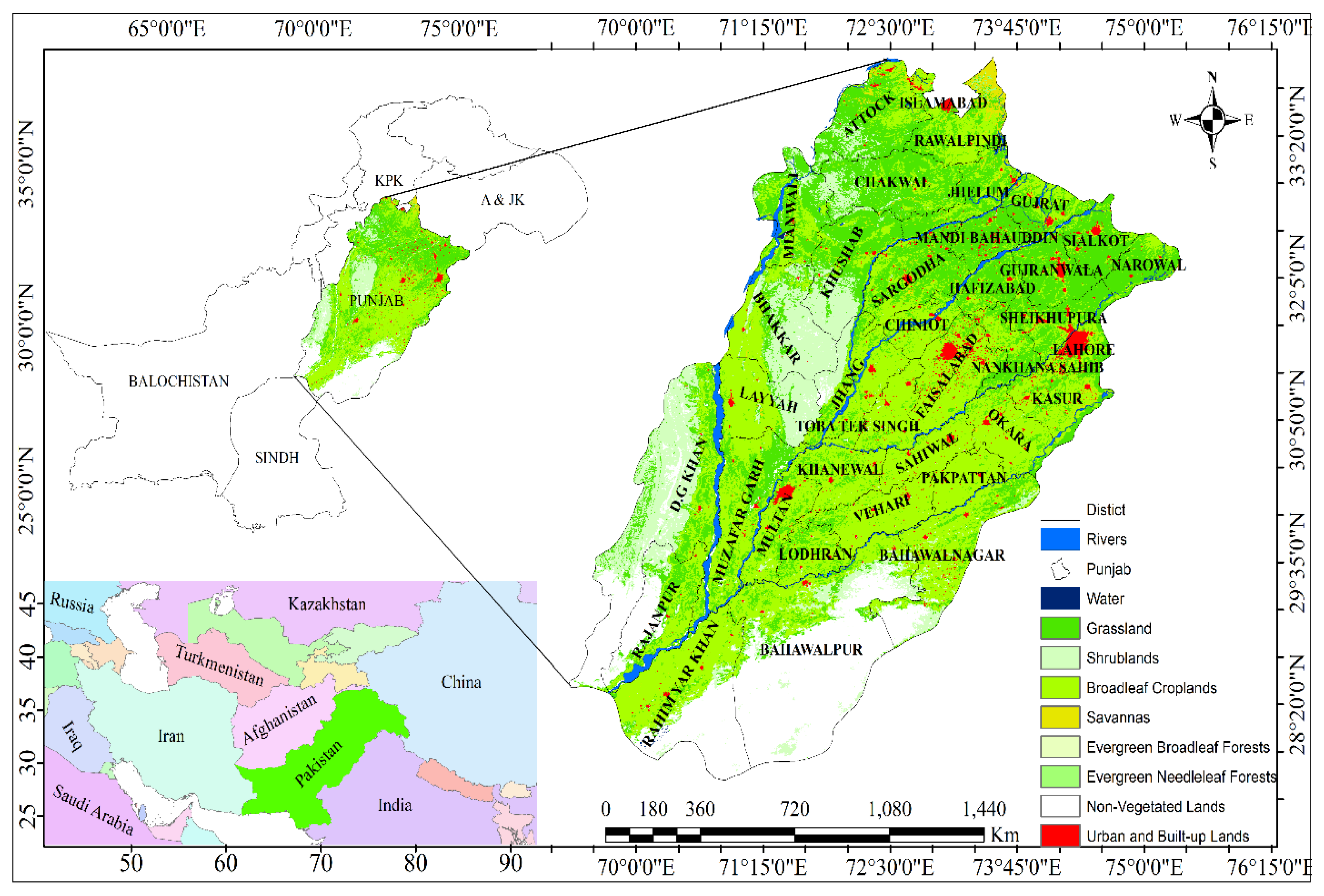Despite these applications, it was suggested that the detection findings of VIs in semi-arid and arid lands should be taken carefully because of the high uncertainty of VIs in thinly vegetative areas, complex vegetation composition, and landscape heterogeneity structure [36,37]. Herein, the performance of vegetation indices SAVI, NDVI, and EVI are assessed for vegetation variability and dynamics in the semi-arid and arid environment of the province of Punjab, Pakistan. We derived NDVI, EVI, and SAVI and related them to their spatiotemporal variability throughout the research area, along with transects because phenological transitions in summer and winter are important factors for changeable crop development and plant growth in spring and autumn [25]. In the present study, two phenological metrics (i.e., for the start of the season and end of the season) were calculated from the MODIS-derived time-series vegetation indices and compared for each vegetation type. Furthermore, the appropriateness of vegetation indices for monitoring the complex vegetation cover in the province of Punjab was evaluated.

2. Materials and Methods

2.1. Study Area

This study was conducted in Punjab Province, Pakistan. It is situated at 27°42′ N to 34°02′ N latitudes and 69°81′ E to 75°23′ E longitudes (Figure 1). According to the area, Punjab is the second largest province in Pakistan, and according to the population, Punjab is ranked number one. Punjab produces wheat, rice, and many other seasonal crops among other provinces. In Punjab, some cities are densely populated. Punjab has 20.63 million hectares of geographical area, almost 12.51 million hectares of cultivated area, and current fallow areas are reported as 2.06 million hectares [38]. Punjab occupies an area of around 205,344 km², with altitudes ranging from 300 m to 2000 m. The north–south length of Punjab Province is long compared to its east to west width. Climate conditions differ from one area to another, depending on the altitude. Punjab is classified into three distinct agroecological zones (i.e., the rain-fed agricultural region of the Potohar Plateau in the north, consisting of 10% of the total agricultural area of the province) (Figure 2) [39]. The limited areas of agricultural production are arid and semi-arid in the province’s southern and central regions, and the Indus Basin’s largest irrigated crop-growing area [40].

2.2. Data Acquisition

Table 1. Datasets used in the present research study.

S. No	Data	Spatial Resolution	Time Period	Source
01	MOD13Q1	250	2000–2019	https://lpdaacsvc.cr.usgs.gov/appeears/ (accessed on 20 May 2020)
02	MCD12Q1	500	2019	https://lpdaacsvc.cr.usgs.gov/appeears/ (accessed on 20 May 2020)
03	Rainfall data		2000–2019	http://www.pmd.gov.pk/ (accessed on 12 August 2020)
04	Temperature data		2000–2019	http://www.pmd.gov.pk/ (accessed on 12 August 2020)

summarizes the datasets used in this study including MODIS time-series data. The three vegetation indices (VIs) used in this study included NDVI, EVI, and SAVI, and all images were extracted from MOD13Q1. All data were acquired from the years 2000 to 2019, which laid the basis for analyzing MODIS time-series data. In particular, a combined time-series of TERRA 16-day composite vegetation indexes (MODIS products MOD13Q1 time-series) at 250 m spatial resolution satellite data was downloaded from the Earth-data (https://lpdaacsvc.cr.usgs.gov/appeears/) (accessed on 20 May 2020) using the Application for Extracting and Exploring Analysis Ready Samples (AρρEEARS) tool to extract data [41,42]. The study area’s annual rainfall and mean temperature data from 2000 to 2019 were acquired from the Pakistan Meteorological Department (PMD) to determine the mean annual rainfall and mean monthly temperature (http://www.pmd.gov.pk/) (accessed on 12 August 2020).

The ArcMap v.10.6 software was used to map and analyze vegetation variability, and ERDAS Imagine 2015 was used for image classification in this study. The shapefile of the respective areas was created, and the area-of-interest (AOI) was extracted by masking using ArcMap v.10.6. image processing tasks and NDVI analysis were accomplished by using ENVI 5.4 [43,44]. The MODIS product (MCD12Q1) of 500 m resolution was used to illustrate the land use and land cover areas. The legend of the International Geosphere-Biosphere Program (IGBP) was also used in the present study. We downloaded the MCD12Q1-2019 from NASA-lpdaac [45].

2.3. Analyzing Vegetation Indices

2.3.1. Vegetation Indices

Three vegetation indices (NDVI, EVI, and SAVI) are widely used to identify vegetation variability, based on the green, blue, red, and NIR bands of MODIS (

Table 2. Vegetation indices used in the study. The G and L values are 2.5 and 0.5, respectively.

Vegetation Indices	Data Source	Formula	References
NDVI	https://lpdaacsvc.cr.usgs.gov/appeears/ (accessed on 20 May 2020)	$\mathrm{NDVI}=\frac{\left(\mathrm{NIR}-\mathrm{RED}\right)}{\left(\mathrm{NIR}+\mathrm{RED}\right)}$	[21,46,47]
SAVI	https://lpdaacsvc.cr.usgs.gov/appeears/ (accessed on 20 May 2020)	$\mathrm{SAVI}=\frac{\left(\mathrm{NIR}-\mathrm{RED}\right)}{\left(\mathrm{NIR}+\mathrm{RED}+\mathrm{L}\right)}\times \left(1+\mathrm{L}\right)$	[48,49]
EVI	https://lpdaacsvc.cr.usgs.gov/appeears/ (accessed on 20 May 2020)	$\mathrm{EVI}=\mathrm{G}\times \frac{\left(\mathrm{NIR}-\mathrm{RED}\right)}{\left(\mathrm{NIR}+6\times \mathrm{RED}-7.5\times \mathrm{BLUE}+1\right)}$	[19]

). These VIs were used to identify mean monthly (from January to December) and mean annual vegetation variability from 2000 to 2019.

2.3.2. Mean Monthly and Annual VIs and Their Variability

The mean monthly VI data based on the 2000 to 2019 time series was used to calculate the mean monthly VIs [50]. Equation (1) was used to calculate every pixel of 20 years of arithmetic mean ${\overline{\mathrm{VI}}}_{\mathrm{m}}$, with n and VI_m represent the number of years and the monthly VIs value, respectively.

$${\overline{\mathrm{VI}}}_{\mathrm{m}}=\frac{1}{\mathrm{n}}{\displaystyle \sum }_1^{\mathrm{n}}\left({\mathrm{VI}}_{\mathrm{m}}\right)$$

(1)

The mean annual calculations of the VIs were used to calculate the mean annual VI (${\overline{\mathrm{VI}}}_{\mathrm{a}}$). To adequately represent vegetation growth, the VIs for the budding season (January to December) were used to calculate the annual mean of VIs and their variation. The deviation (${\mathrm{DVI}}_{\mathrm{i}}$) from the years 2000 to 2019, mean annual VIs at a given spatial location for a certain year i was calculated using the following equation.

$${\mathrm{DVI}}_{\mathrm{i}}={\mathrm{VI}}_{\mathrm{i}}-{\overline{\mathrm{VI}}}_{\mathrm{a}}$$

(2)

Furthermore, the relative annual VI deviation (${\mathrm{rDVI}}_{\mathrm{i}}$) was estimated using the following equation, which defines the deviation as a percentage of the mean annual VIs:

$${\mathrm{rDVI}}_{\mathrm{i}}=\frac{{\mathrm{DVI}}_{\mathrm{i}}\times 100}{{\overline{\mathrm{VI}}}_{\mathrm{a}}}$$

(3)

The annual mean of VIs variability ($\overline{\mathrm{VVI}}$) was estimated with the relative annual VI deviation (${\mathrm{rDVI}}_{\mathrm{i}}$), with n being the number of years using the following equation.

$$\overline{\mathrm{VVI}}=\frac{1}{\mathrm{n}}{\displaystyle \sum }_1^{\mathrm{n}}\left|{\mathrm{rDVI}}_{\mathrm{i}}\right|$$

(4)

2.4. Detection of Phenological Metrics

The TIMESAT software is a popular tool for the study of time-series data [51]. Given the variability of the VIs time-series, TIMESAT’s curve approach has the best suitable noise reduction efficiency and signal integrity maintenance. Reliable results were obtained using TIMESAT for most vegetation forms identified by the three VIs [37,52]. The TIMESAT software was used to smooth out the time-series of VIs and calculate the phenological metrics for the study area. Other functions of the local Gaussian type were used for data at intervals around the time-series minimum and maximum. Two phenological metrics were analyzed and mapped for all VIs time-series, namely, the start of the season and the end of the season.

Table 3. Description of phenological metrics.

Metric	Definition
Start of the season	Time for which the left edge has increased to 30% of the seasonal amplitude measured from the left minimum level.
End of the season	Time for which the right edge has decreased to 30% of the seasonal amplitude measured from the right minimum level.

lists the identified phenological metrics and their descriptions [51].

3. Results

3.1. Vegetation Indices

3.1.1. Mean Monthly VIs

The mean monthly NDVI for the period from 2000 to 2019 and the months from January to December are shown in Figure 3. Mean monthly VIs indicate a growing cycle throughout the year of various vegetation types, and two growing seasons can be seen, winter (Rabi) and summer (Kharif). The first part (Rabi) shows that vegetation growth starts in October and November. The second part (Kharif) indicates another vegetation growth season commencing in late April to the first week of May in the study area. From late December to the first week of January, the vegetation in the entire area tends to be senescent. Low NDVI values were also observed from April to July and October to November.

Seasonal mean monthly dynamics of vegetation indices demonstrate seasonal growth of the vegetation, representing the trend of development for different types of vegetation. The agricultural area showed high vegetation activity during both seasons (Rabi and Kharif), while low vegetation from April to July and October to November in many parts of the study area was observed.

3.1.2. Mean Annual VIs

The mean annual NDVI, EVI, and SAVI from 2000 to 2019 indicated identical spatial trends for different landscape situations described above, but differed in spatial vigor (Figure 4). All VIs represented a regional trend of strong VIs for the northwest and southeast of the study area and small values for the industrial and suburban areas. Maximum annual VI trend was observed in the eastern, central, and southeastern parts of the study area.

The spatial variability of annual mean VIs was consistent with regional climate conditions in northern and southern Punjab (Figure 4). With greater rainfall in northern parts, an increasing trend in vegetation (trees, grasslands, and farm ground) forms longer growing seasons. Figure 5 displays the mean annual variation in the VIs for the period from 2000 to 2019. It shows spatial variations of annual mean VIs from one year to the next, which can be used for monitoring purposes.

In comparison, in southern Punjab, relatively small growing seasons are starting in the desert area. In this region, vegetation growth is limited throughout the year by low precipitation. The NDVI image displays higher values in most instances than the images in the EVI and SAVI time series. In the northern part of Punjab, dense coniferous forests are found in high mountains with large annual precipitation. Grasslands have spread almost throughout the entire Punjab; NDVI displayed higher mean annual values than EVI and SAVI time-series images. To highlight the spatial variations in distinctive eco-regions between the NDVI, EVI, and SAVI, three large transects were used as samples within the mean VIs time-series images of the year (Figure 4).

All transects start with sparse vegetation and cross heavily vegetated areas to cover a wide variety of VI values, except transect c. All these transects include forests, croplands, grasslands, savanna, and barren land. Similar patterns can be found between the VI profiles (Figure 5). Nevertheless, the NDVI profiles observed wider data ranges than the EVI and SAVI profiles.

Transect a starts from the northwestern forest area near Attock and ends in the east–southeast cropland areas and is about 400 miles long. Mostly barren land, cropland, and grassland are found in this transect region. The transect extends to cropland, sparse grassland, and crosses the barren area in the district of Chakwal, showing very low VI values. Transect b starts from sparse grassland and cropland areas in the central Punjab, crosses a mix of forest, sparse vegetation, and agricultural area in central Punjab, and ends in the cropland areas. NDVI and SAVI display high VI values compared to EVI values in this area.

Transect c follows the north to south latitude line from 34° N to 29° N and is about 800 km long. A small part of grassland and highly evergreen needle leaf forest characterize the northern part of the transect, where SAVI and NDVI showed high variation, whereas EVI had little variation. The VI values were higher between 33° N and 34° N and showed a rather smooth behavior. This area was also categorized as homogeneous, mainly forest, cropland, and grassland cover. The higher values of VIs were found in northwestern Punjab between 33° N and 34° N latitudes, parallel to the agricultural areas, forests, and steppe along the mountains. The VIs values were lower in the zone between 33° N and 32° N due to barren land and shrublands. Barren land was mostly observed on the western side of this zone. Barren terrain and cropland were observed between 31° N and 32° N latitudes. Annual and seasonal variability were found in transect c. The VIs of the grassland located in the district of Chakwal was meaningfully less than that of the barren land and grassland between 29° N and 30° N latitudes due to the highly arid climate and very sparse vegetation.

The EVI map showed maximum variability (

Table 4. Mean annual VI variability in percentage for 2000 to 2019.

Percentage	NDVI	EVI	SAVI
0–10%	7.03	3.82	6.95
10–20%	18.53	30.23	17.85
20–30%	13.54	28.23	15.02
30–40%	19.29	23.44	17.65
>40%	41.61	14.28	42.53

) by equating the three variability maps quantitatively. The NDVI time-series thus captured greater inter-annual variation for the entire Punjab Province from 2000 to 2019 compared to EVI and SAVI. Given the high vegetation in the northern area near the river, the high variability observed in this area only from EVI data could be due to the variations in soil background properties.

3.2. Phenological Metrics Detection

The phenological metrics of the start of the season and the end of the season over the Punjab Province were mapped from 2000 to 2019 using the NDVI, EVI, and SAVI time-series MODIS data. Their standard deviation (SD) and mean for each type of vegetation from the three VI datasets is shown in

Table 5. Phenological metrics detected by VIs over the study area for 2000–2019.

S. No	Vegetation Classes	$\mathbf{S}\mathbf{O}{\mathbf{S}}_{\mathbf{N}\mathbf{D}\mathbf{V}\mathbf{I}}$		$\mathbf{E}\mathbf{O}{\mathbf{S}}_{\mathbf{N}\mathbf{D}\mathbf{V}\mathbf{I}}$		$\mathbf{S}\mathbf{O}{\mathbf{S}}_{\mathbf{E}\mathbf{V}\mathbf{I}}$		$\mathbf{E}\mathbf{O}{\mathbf{S}}_{\mathbf{E}\mathbf{V}\mathbf{I}}$		$\mathbf{S}\mathbf{O}{\mathbf{S}}_{\mathbf{S}\mathbf{A}\mathbf{V}\mathbf{I}}$		$\mathbf{E}\mathbf{O}{\mathbf{S}}_{\mathbf{S}\mathbf{A}\mathbf{V}\mathbf{I}}$
		Mean	SD	Mean	SD	Mean	SD	Mean	SD	Mean	SD	Mean	SD
1	Grassland	120.3	33.4	116.9	28.3	118.4	29.5	293.8	28.7	313.4	27.8	290.2	40.7
2	Evergreen Broadleaf Forests	115.9	27.3	113.5	26.9	116.9	27.8	29.5	26.8	306.2	26.9	288.3	33.5
3	Evergreen Needleleaf Forests	116.5	28.3	111.2	23.5	111.9	22.3	286.4	23.4	308.9	27.7	280.3	27.2
4	Shrublands	140.3	26.8	133.8	22.9	135.8	23.5	310.3	27.9	330.5	27.8	307.5	34.8
5	Cropland	138.3	22.3	133.3	23.6	132.6	21.5	308.7	19.3	314.5	18.2	302.3	20.3
6	Savanna	123.3	33.2	121.5	18.3	121.5	17.4	302.3	15.6	309.5	15.2	299.5	39.5
7	Mixed Forests	126.3	17.9	121.3	14.3	118.3	12.3	299.7	16.9	315.3	14.4	286.5	26.2

. The normal standard deviation at the start of the season ranged from 12.3 days to 33.4 days. The default end-of-season deviation ranged from 14.4 days to 40.7 days. Except for forest, the NDVI end of season exhibited a strong deviation from EVI and SAVI. Except for savanna and shrublands, the start of the season from the NDVI, MODIS time series showed greater deviation than EVI and SAVI.

Figure 6 illustrates the two-phonology metrics for different vegetation types. Despite the peak change, the season start and season-end distributions of the histograms from the three VIs agreed. Comprehensible bimodal dispersals are seen for the grassland season start, cropland season start, and season-end cropland. The bimodal cropland starts from the season and distribution at the end of the season, suggesting diverse phenological trends for dissimilar crop types because of the bare soil’s effect on the vegetation index [53]. Different density grasslands and vegetation cover may exhibit varying green-up behaviors, causing the bimodal start of season distribution. Discrepancies for grassland start of the season, evergreen leaf forest end of the season, and grassland end of the season were observed from three VIs. $Startofseaso{n}_{NDVI}$ had a high peak and a secondary peak at MOD13Q1 for grassland, whereas the $startofseaso{n}_{NDVI}$ had two parallel peaks. Similar disagreements were noted at the grassland end of the season. $Endofseaso{n}_{EVI}$ had bimodal distribution for the evergreen needleaf forest as associated with the unimodal dispersal of $Endofseaso{n}_{NDVI}$ and $endofseaso{n}_{EVI}$. The values spread near the histogram’s tail indicate over estimations of evergreen needle leaf forest, mixed forest, savanna, grassland, and shrubland at the $end of seaso{n}_{NDVI}$.

4. Discussion

This approach is used to map and identify vegetation variability distributions.

4.1. VI Variability

Various factors including clouds and shadow-polluted pixels, time-based interpolation, smoothing, spatial filtering, cropping assumptions, and mixed pixels can influence the VI values. NDVI and SAVI are more prone to atmospheric effects than EVI, induced by cloud presence. The impurity of the peaks of the remaining clouds makes a big difference in NDVI values. Some limitations in the MODIS cloud mask exist even after using it to decrease cloud properties on per-pixel surface reflectance [54,55]. Vegetation shifts are misidentified with EVI, degraded by the presence of clouds and aerosols [56]. The reliability of quantified vegetation variations mainly depends on how image classification incorporates atmospheric and cloud transmission information. Affected pixels may be treated by additional masking [56], which targets the resulting inconsistencies through quantifying vegetation variability using the NDVI time series. High VI variation (>40%) can be seen in areas near water bodies, and low vegetation occurs near built-up areas (Figure 4) [54,55]. VI variation (10–30%) occurs in the vicinity of the river, and the majority of cropland areas occur in the study area. This variation may be due to a combination of minor crop fields. In sparsely vegetated areas, in particular, EVI has more coverage than SAVI and NDVI. The soil composition of these regions largely consists of dry sand. NDVI has been described as vulnerable to the spectral effect of soil moisture and texture in the spaces between desert grassland and shrubland [57,58]. The great annual diversity observed from EVI may be correlated with a difference in soil history at low levels of VIs.

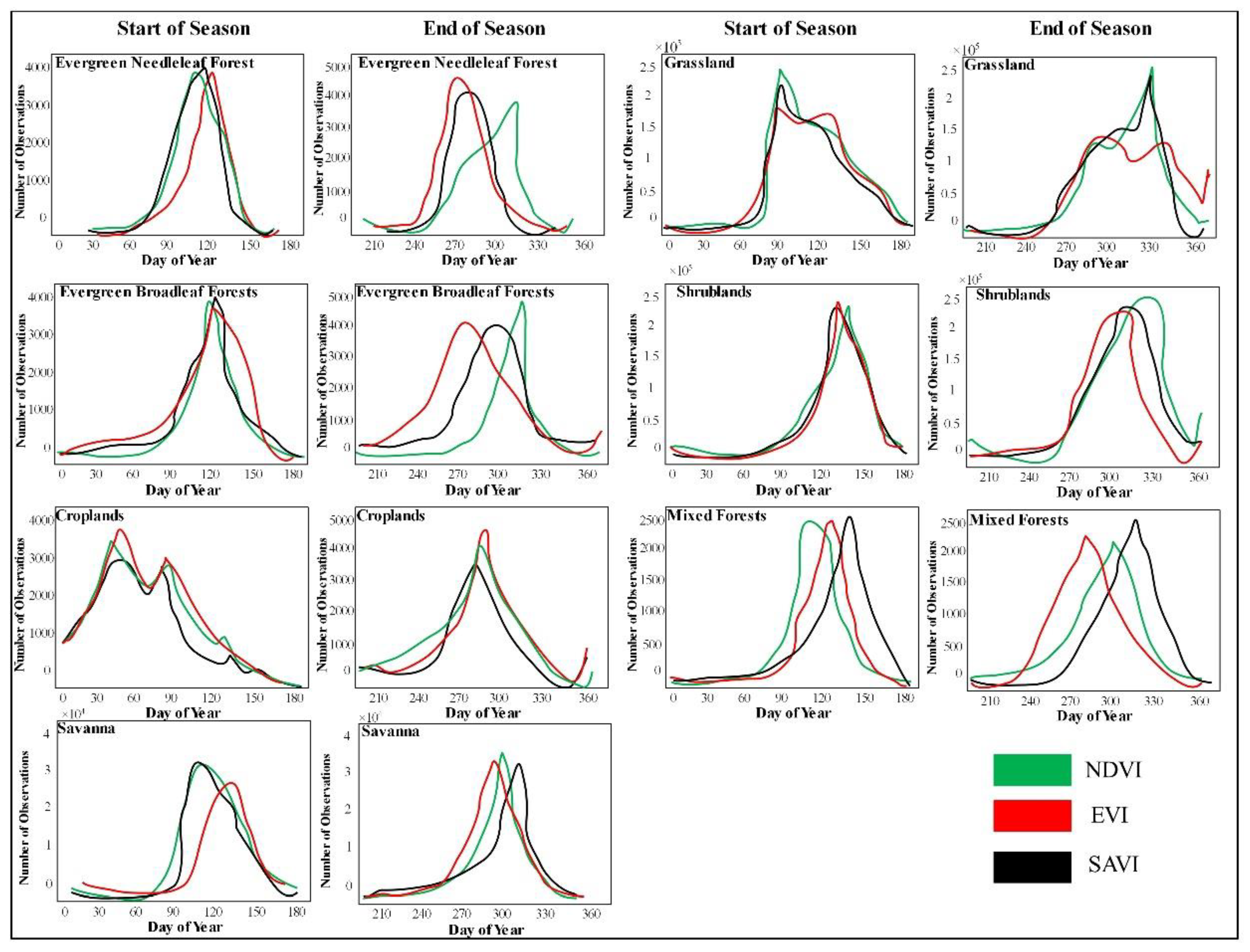
4.2. Detection of Phenology Metrics

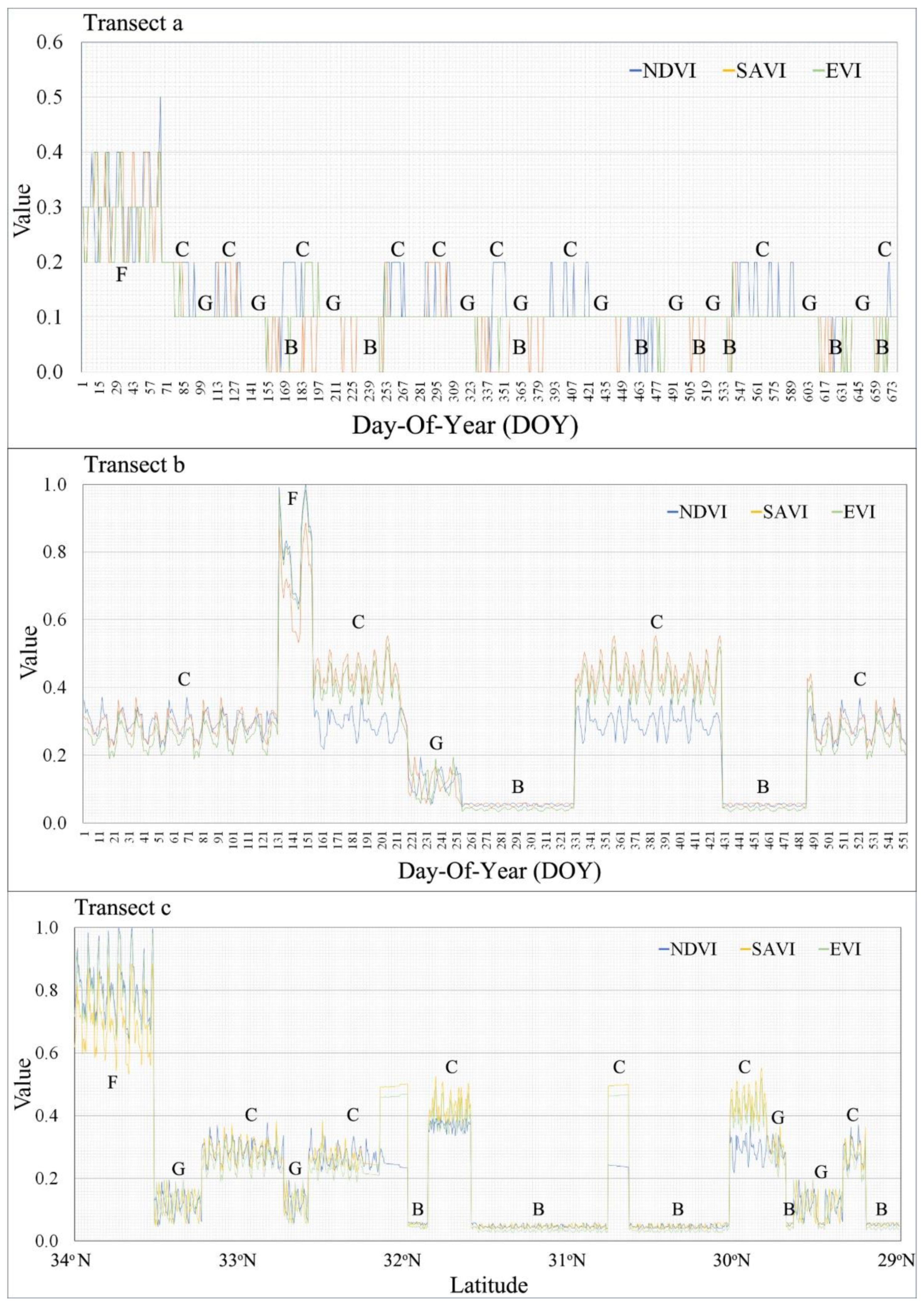
Using TIMESAT’s curve-fitting approach with an equal seasonal amplitude threshold (40%), different VI dynamic phenological metrics were detected for Punjab Province (Figure 6). Despite the indecision of the VIs time-series, TIMESAT has obtained good results from the three VIs for most vegetation types. The results of the three VIs in this study follow that of previous studies [12,29], demonstrating their efficiency for phenological metrics recognition in arid and semi-arid environments. There are, however, still some inconsistencies in the findings of phenology detection. In our analysis, the variability at the end of the season observed from MODIS VIs was greater than that at the start of the season (Table 4), consistent with earlier studies [59,60].

The greatest variance in phenological metrics was observed from the NDVI time series. The overestimation of the end of the season exhibited high variability rates because of its vulnerability to atmospheric conditions and soil composition. The difference between histogram dispersals of phenological metrics of estimated VIs may be due to their varying sensitivities to soil context variations. Likewise, in the drylands of Arizona, USA, the spatiotemporal variability of soil surface phenology removed from NDVI was higher than EVI [61]. The difference in highest greenness between NDVI and EVI was related to the physiological features of the vegetation types due to their different sensitivities [36]. More comprehensive information is required for the improved assessment of the suitability of VIs in a dryland environment for phenological detection. Our understanding of ecosystem processes over the arid landscape would be useful for evaluating satellite-derived phenological metrics with measurements of flux tower footprint CO₂ or in situ VI extents [62,63].

In the present research, the limitation of data acquisition throughout situ precludes further review. Furthermore, in our study, we compared only three widely used VIs. Furthermore, the utility of other vegetation indices such as the optimized soil adjusted vegetation index (OSAVI), EVI2, and MSAVI, and their combined use can be of significance for complex vegetation cover investigations in the arid and semi-arid regions.

One of the limitations of the approach taken in this study is that it is rigid (i.e., it assumes that the time series oscillates at a regular interval over the year). Additionally, remote sensing vegetation indices were more closely associated with the formation of the canopy structure in the spring, and persistence after photosynthesis ceased in autumn. Additionally, low fractional vegetation cover in the south of the study area was a primary limitation so site-specific circumstances such as the considerable spatial heterogeneity of pixels generated by the sparse vegetation were a source of uncertainty. Sites with short growth seasons and a scarcity of high-quality observations would make it even more difficult to extract seasonal patterns. Moreover, the spatial patterns of the VI-derived phenology agreed well with the timing of the start, end, and length of season, but uncertainties appeared in areas with limited seasonality expressed in the satellite signal and systematic biases.

5. Conclusions

An approach was implemented to identify vegetation variability and its dynamics by comprehensively using three vegetation indices (EVI, SAVI, and NDVI) estimated through MODIS time-series data in the Punjab Province of Pakistan. The varying associations of NDVI, EVI, and SAVI were estimated in different vegetation forms. A minor correlation exists between NDVI, EVI, and SAVI, with Pearson’s correlation coefficients ranging from 0.42 to 0.50. Due to the blue band reflectance disturbance, EVI typically showed high uncertainties in sparse vegetation areas of grassland and forest. The EVI time-series showed the highest inter-annual variability in Punjab from 2000 to 2019, with 14.28% of the total region showing higher variability than 40%. For most vegetation types, the phenological metrics of season-start and season-end generated by the NDVI, SAVI, and EVI were consistent. The greatest deviations from phenological metrics were obtained from the NDVI time-series (33.4 days at the start of the season and 40.7 days at the end of the season), suggesting soil context-sensitivity and atmospheric effects of the index. The annual mean VI images displayed parallel spatial arrangements of vegetation conditions with fluctuating levels. Major steps include using the temporal interpolation algorithm to remove contaminated pixels to reconstruct MODIS NDVI time-series data. The EVI time-series showed greater inter-annual variations from 2000 to 2019 compared to SAVI and NDVI. Given the high vegetation variability in northern Punjab, the high variability in EVI values could be due to variations in soil background properties. In the future, to assess the climatic effect on semi-arid, arid, and rainfed areas’ vegetation dynamics, satellite data will be assessed along with climate data for the region and other larger areas.

References

1. Sharifi, A.; Amini, J.; Pourshakouri, F. Development of an allometric model to estimate above-ground biomass of forests using MLPNN algorithm, case study: Hyrcanian forests of Iran. Casp. J. Environ. Sci. 2016, 14, 125–137. [Google Scholar]
2. Reynolds, J.F.; Stafford Smith, D.M.; Lambin, E.F.; Turner, B.L.; Mortimore, M.; Batterbury, S.P.J.; Downing, T.E.; Dowlatabadi, H.; Fernández, R.J.; Herrick, J.E.; et al. Ecology: Global desertification: Building a science for dryland development. Science 2007, 316, 847–851. [Google Scholar] [CrossRef] [Green Version]
3. Herrmann, S.M.; Anyamba, A.; Tucker, C.J. Recent trends in vegetation dynamics in the African Sahel and their relationship to climate. Glob. Environ. Chang. 2005, 15, 394–404. [Google Scholar] [CrossRef]
4. Wessels, K.J.; Prince, S.D.; Malherbe, J.; Small, J.; Frost, P.E.; VanZyl, D. Can human-induced land degradation be distinguished from the effects of rainfall variability? A case study in South Africa. J. Arid Environ. 2007, 68, 271–297. [Google Scholar] [CrossRef]
5. Gibbes, C.; Southworth, J.; Waylen, P.; Child, B. Climate variability as a dominant driver of post-disturbance savanna dynamics. Appl. Geogr. 2014, 53, 389–401. [Google Scholar] [CrossRef]
6. Seaquist, J.W.; Hickler, T.; Eklundh, L.; Ardö, J.; Heumann, B.W. Disentangling the effects of climate and people on Sahel vegetation dynamics. Biogeosci. Discuss. 2008, 5, 3045–3067. [Google Scholar] [CrossRef]
7. Tariq, A.; Shu, H.; Kuriqi, A.; Siddiqui, S.; Gagnon, A.S.; Lu, L.; Linh, N.T.T.; Pham, Q.B. Characterization of the 2014 Indus River Flood Using Hydraulic Simulations and Satellite Images. Remote Sens. 2021, 13, 2053. [Google Scholar] [CrossRef]
8. Zhou, L.; Tucker, C.J.; Kaufmann, R.K.; Slayback, D.; Shabanov, N.V.; Myneni, R.B. Variations in northern vegetation activity inferred from satellite data of vegetation index during 1981 to 1999. J. Geophys. Res. Atmos. 2001, 106, 20069–20083. [Google Scholar] [CrossRef]
9. Morisette, J.T.; Richardson, A.D.; Knapp, A.K.; Fisher, J.I.; Graham, E.A.; Abatzoglou, J.; Wilson, B.E.; Breshears, D.D.; Henebry, G.M.; Hanes, J.M.; et al. Tracking the rhythm of the seasons in the face of global change: Phenological research in the 21st century. Front. Ecol. Environ. 2009, 7, 253–260. [Google Scholar] [CrossRef] [Green Version]
10. Goetz, S.J.; Prince, S.D. Modelling Terrestrial Carbon Exchange and Storage: Evidence and Implications of Functional Convergence in Light-use Efficiency. Adv. Ecol. Res. 1999, 28, 57–92. [Google Scholar] [CrossRef]
11. Yan, C.Z.; Wang, T.; Han, Z.W.; Qie, Y.F. Surveying sandy deserts and desertified lands in north-western China by remote sensing. Int. J. Remote Sens. 2007, 28, 3603–3618. [Google Scholar] [CrossRef]
12. Hazaymeh, K.; Hassan, Q.K.; Hazaymeh, K.; Hassan, Q.K. Remote sensing of agricultural drought monitoring: A state of art review. AIMS Environ. Sci. 2016, 3, 604–630. [Google Scholar] [CrossRef]
13. Wilson, N.R.; Norman, L.M.; Villarreal, M.; Gass, L.; Tiller, R.; Salywon, A. Comparison of remote sensing indices for monitoring of desert cienegas. Arid L. Res. Manag. 2016, 30, 460–478. [Google Scholar] [CrossRef] [Green Version]
14. Ghaderizadeh, S.; Abbasi-Moghadam, D.; Sharifi, A.; Zhao, N.; Tariq, A. Hyperspectral image classification using a hybrid 3D-2D convolutional neural networks. IEEE J. Sel. Top. Appl. Earth Obs. Remote Sens. 2021, 14, 7570–7588. [Google Scholar] [CrossRef]
15. Weiss, J.L.; Gutzler, D.S.; Coonrod, J.E.A.; Dahm, C.N. Long-term vegetation monitoring with NDVI in a diverse semi-arid setting, central New Mexico, USA. J. Arid Environ. 2004, 58, 249–272. [Google Scholar] [CrossRef]
16. Tucker, C.J.; Pinzon, J.E.; Brown, M.E.; Slayback, D.A.; Pak, E.W.; Mahoney, R.; Vermote, E.F.; El Saleous, N. An extended AVHRR 8-km NDVI dataset compatible with MODIS and SPOT vegetation NDVI data. Int. J. Remote Sens. 2005, 26, 4485–4498. [Google Scholar] [CrossRef]
17. Fensholt, R.; Sandholt, I. Evaluation of MODIS and NOAA AVHRR vegetation indices with in situ measurements in a semi-arid environment. Int. J. Remote Sens. 2005, 26, 2561–2594. [Google Scholar] [CrossRef]
18. Wu, W. The Generalized Difference Vegetation Index (GDVI) for dryland characterization. Remote Sens. 2014, 6, 1211–1233. [Google Scholar] [CrossRef] [Green Version]
19. Huete, A. Overview of the radiometric and biophysical performance of the MODIS vegetation indices. Remote Sens. Environ. 2002, 83, 195–213. [Google Scholar] [CrossRef]
20. Huete, A.R.; Jackson, R.D.; Post, D.F. Spectral response of a plant canopy with different soil backgrounds. Remote Sens. Environ. 1985, 17, 37–53. [Google Scholar] [CrossRef]
21. Huete, A.R. A soil-adjusted vegetation index (SAVI). Remote Sens. Environ. 1988, 25, 295–309. [Google Scholar] [CrossRef]
22. Qi, J.; Chehbouni, A.; Huete, A.R.; Kerr, Y.H.; Sorooshian, S. A modified soil adjusted vegetation index. Remote Sens. Environ. 1994, 48, 119–126. [Google Scholar] [CrossRef]
23. Rondeaux, G.; Steven, M.; Baret, F. Optimization of soil-adjusted vegetation indices. Remote Sens. Environ. 1996, 55, 95–107. [Google Scholar] [CrossRef]
24. Mumtaz, F.; Tao, Y.; De Leeuw, G.; Zhao, L.; Fan, C.; Elnashar, A.; Bashir, B.; Wang, G.; Li, L.L.; Naeem, S.; et al. Modeling spatio-temporal land transformation and its associated impacts on land surface temperature (LST). Remote Sens. 2020, 12, 2987. [Google Scholar] [CrossRef]
25. Richardson, A.D.; Black, T.A.; Ciais, P.; Delbart, N.; Friedl, M.A.; Gobron, N.; Hollinger, D.Y.; Kutsch, W.L.; Longdoz, B.; Luyssaert, S.; et al. Influence of spring and autumn phenological transitions on forest ecosystem productivity. Philos. Trans. R. Soc. B Biol. Sci. 2010, 365, 3227–3246. [Google Scholar] [CrossRef] [Green Version]
26. Tariq, A.; Shu, H. CA-Markov Chain Analysis of Seasonal Land Surface Temperature and Land Use Landcover Change Using Optical Multi-Temporal Satellite Data of Faisalabad, Pakistan. Remote Sens. 2020, 12, 3402. [Google Scholar] [CrossRef]
27. Motohka, T.; Nasahara, K.N.; Miyata, A.; Mano, M.; Tsuchida, S. Evaluation of optical satellite remote sensing for rice paddy phenology in monsoon Asia using a continuous in situ dataset. Int. J. Remote Sens. 2009, 30, 4343–4357. [Google Scholar] [CrossRef]
28. Motohka, T.; Nasahara, K.N.; Oguma, H.; Tsuchida, S. Applicability of Green-Red Vegetation Index for remote sensing of vegetation phenology. Remote Sens. 2010, 2, 2369–2387. [Google Scholar] [CrossRef] [Green Version]
29. Nagai, S.; Saitoh, T.M.; Kobayashi, H.; Ishihara, M.; Suzuki, R.; Motohka, T.; Nasahara, K.N.; Muraoka, H. In situ examination of the relationship between various vegetation indices and canopy phenology in an evergreen coniferous forest, Japan. Int. J. Remote Sens. 2012, 33, 6202–6214. [Google Scholar] [CrossRef]
30. Zainab, N.; Tariq, A.; Siddiqui, S. Development of Web-Based GIS Alert System for Informing Environmental Risk of Dengue Infections in Major Cities of Pakistan. Geosfera Indones. 2021, 6, 77. [Google Scholar] [CrossRef]
31. Rocha, A.V.; Shaver, G.R. Advantages of a two band EVI calculated from solar and photosynthetically active radiation fluxes. Agric. For. Meteorol. 2009, 149, 1560–1563. [Google Scholar] [CrossRef]
32. Bannari, A.; Morin, D.; Bonn, F.; Huete, A.R. A review of vegetation indices. Remote Sens. Rev. 1995, 13, 95–120. [Google Scholar] [CrossRef]
33. Rodríguez-Moreno, V.M.; Bullock, S.H. Vegetation response to hydrologic and geomorphic factors in an arid region of the Baja California Peninsula. Environ. Monit. Assess. 2014, 186, 1009–1021. [Google Scholar] [CrossRef] [PubMed] [Green Version]
34. Sjöström, M.; Ardö, J.; Eklundh, L.; El-Tahir, B.A.; El-Khidir, H.A.M.; Hellström, M.; Hellström, M.; Seaquist, J. Evaluation of satellite based indices for gross primary production estimates in a sparse savanna in the Sudan. Biogeosciences 2009, 6, 129–138. [Google Scholar] [CrossRef] [Green Version]
35. Ghaderpour, E.; Vujadinovic, T. The Potential of the Least-Squares Spectral and Cross-Wavelet Analyses for Near-Real-Time Disturbance Detection within Unequally Spaced Satellite Image Time Series. Remote Sens. 2020, 12, 2446. [Google Scholar] [CrossRef]
36. Walker, J.; de Beurs, K.; Wynne, R.H. Phenological response of an Arizona dryland forest to short-term climatic extremes. Remote Sens. 2015, 7, 10832–10855. [Google Scholar] [CrossRef] [Green Version]
37. Hird, J.N.; McDermid, G.J. Noise reduction of NDVI time series: An empirical comparison of selected techniques. Remote Sens. Environ. 2009, 113, 248–258. [Google Scholar] [CrossRef]
38. Tariq, A.; Shu, H.; Siddiqui, S.; Imran, M.; Farhan, M. Monitoring Land Use And Land Cover Changes Using Geospatial Techniques, A Case Study Of Fateh Jang, Attock, Pakistan. Geogr. Environ. Sustain. 2021, 14, 41–52. [Google Scholar] [CrossRef]
39. Qasim, M. Determinants of Farm Income and Agricultural Risk Management Strategies: The Case of Rain-Fed Farm Households in Pakistan’s Punjab; Kassel University Press: Kassel, Germany, 2012; Volume 3, ISBN 9783862192984. [Google Scholar]
40. Khan, A.; Hansen, M.; Potapov, P.; Adusei, B.; Pickens, A.; Krylov, A.; Stehman, S. Evaluating Landsat and RapidEye Data for Winter Wheat Mapping and Area Estimation in Punjab, Pakistan. Remote Sens. 2018, 10, 489. [Google Scholar] [CrossRef] [Green Version]
41. Busetto, L.; Zwart, S.J.; Boschetti, M. Analysing spatial–temporal changes in rice cultivation practices in the Senegal River Valley using MODIS time-series and the PhenoRice algorithm. Int. J. Appl. Earth Obs. Geoinf. 2019, 75, 15–28. [Google Scholar] [CrossRef]
42. Tariq, A.; Riaz, I.; Ahmad, Z. Land surface temperature relation with normalized satellite indices for the estimation of spatio-temporal trends in temperature among various land use land cover classes of an arid Potohar region using Landsat data. Environ. Earth Sci. 2020, 79, 1–15. [Google Scholar] [CrossRef]
43. Mohamed, N.; Bannari, A. The Relationship between Vegetation and Rainfall in Central Sudan. Int. J. Remote Sens. Appl. 2016, 6, 30. [Google Scholar] [CrossRef]
44. Imran, M.; Basit, I.; Khan, M.R.; Ahmad, S.R. Analyzing the Impact of Spatio-Temporal Climate Variations on the Rice Crop Calendar in Pakistan. Int. J. Biol. Life Agric. Sci. 2018, 12, 177–184. [Google Scholar] [CrossRef]
45. Friedl, M.A.; Sulla-Menashe, D.; Tan, B.; Schneider, A.; Ramankutty, N.; Sibley, A.; Huang, X. MODIS Collection 5 global land cover: Algorithm refinements and characterization of new datasets. Remote Sens. Environ. 2010, 114, 168–182. [Google Scholar] [CrossRef]
46. Matsushita, B.; Yang, W.; Chen, J.; Onda, Y.; Qiu, G. Sensitivity of the Enhanced Vegetation Index (EVI) and Normalized Difference Vegetation Index (NDVI) to topographic effects. Sensors 2007, 7, 2636–2651. [Google Scholar] [CrossRef] [PubMed] [Green Version]
47. Gu, Y.; Hunt, E.; Wardlow, B.; Basara, J.B.; Brown, J.F.; Verdin, J.P. Evaluation of MODIS NDVI and NDWI for vegetation drought monitoring using Oklahoma Mesonet soil moisture data. Geophys. Res. Lett. 2008, 35. [Google Scholar] [CrossRef] [Green Version]
48. Huete, A.R.; Jackson, R.D. Soil and atmosphere influences on the spectra of partial canopies. Remote Sens. Environ. 1988, 25, 89–105. [Google Scholar] [CrossRef]
49. Jensen, J. Introductory Digital Image Processing: A Remote Sensing Perspective, Third Edition. Environ. Eng. Geosci. 1996, 13, 89–90. [Google Scholar] [CrossRef]
50. Shah, S.H.I.A.; Yan, J.; Ullah, I.; Aslam, B.; Tariq, A.; Zhang, L.; Mumtaz, F. Classification of Aquifer Vulnerability by Using the DRASTIC Index and Geo-Electrical Techniques. Water 2021, 13, 2144. [Google Scholar] [CrossRef]
51. Jönsson, P.; Eklundh, L. TIMESAT—A program for analyzing time-series of satellite sensor data. Comput. Geosci. 2004, 30, 833–845. [Google Scholar] [CrossRef] [Green Version]
52. Wang, C.; Fritschi, F.B.; Stacey, G.; Yang, Z. Phenology-based assessment of perennial energy crops in North American tallgrass prairie. Ann. Assoc. Am. Geogr. 2011, 101, 742–751. [Google Scholar] [CrossRef]
53. Lu, L.; Kuenzer, C.; Guo, H.; Li, Q.; Long, T.; Li, X. A novel land cover classification map based on a modis time-series in Xinjiang, China. Remote Sens. 2014, 6, 3387–3408. [Google Scholar] [CrossRef] [Green Version]
54. Liu, J.; Zhang, W.; Liu, T. Monitoring recent changes in snow cover in Central Asia using improved MODIS snow-cover products. J. Arid Land 2017, 9, 763–777. [Google Scholar] [CrossRef]
55. Wilson, A.M.; Parmentier, B.; Jetz, W. Systematic land cover bias in Collection 5 MODIS cloud mask and derived products—A global overview. Remote Sens. Environ. 2014, 141, 149–154. [Google Scholar] [CrossRef]
56. Samanta, A.; Ganguly, S.; Myneni, R.B. MODIS enhanced vegetation index data do not show greening of amazon forests during the 2005 drought. New Phytol. 2011, 189, 11–15. [Google Scholar] [CrossRef] [PubMed]
57. Kremer, R.G.; Running, S.W. Community type differentiation using NOAA/AVHRR data within a sagebrush-steppe ecosystem. Remote Sens. Environ. 1993, 46, 311–318. [Google Scholar] [CrossRef]
58. Schmidt, H.; Karnieli, A. Remote sensing of the seasonal variability of vegetation in a semi-arid environment. J. Arid Environ. 2000, 45, 43–59. [Google Scholar] [CrossRef] [Green Version]
59. Lu, L.; Wang, C.; Guo, H.; Li, Q. Detecting winter wheat phenology with SPOT-VEGETATION data in the North China Plain. Geocarto Int. 2014, 29, 244–255. [Google Scholar] [CrossRef]
60. Zhang, X.; Friedl, M.A.; Schaaf, C.B. Global vegetation phenology from Moderate Resolution Imaging Spectroradiometer (MODIS): Evaluation of global patterns and comparison with in situ measurements. J. Geophys. Res. Biogeosci. 2006, 111, 1–14. [Google Scholar] [CrossRef]
61. Shang, R.; Liu, R.; Xu, M.; Liu, Y.; Dash, J.; Ge, Q. Determining the start of the growing season from MODIS data in the Indian Monsoon Region: Identifying available data in the rainy season and modeling the varied vegetation growth trajectories. Remote Sens. 2018, 10, 122. [Google Scholar] [CrossRef] [Green Version]
62. Jones, M.O.; Kimball, J.S.; Jones, L.A.; McDonald, K.C. Satellite passive microwave detection of North America start of season. Remote Sens. Environ. 2012, 123, 324–333. [Google Scholar] [CrossRef]
63. Hmimina, G.; Dufrêne, E.; Pontailler, J.Y.; Delpierre, N.; Aubinet, M.; Caquet, B.; de Grandcourt, A.; Burban, B.; Flechard, C.; Granier, A.; et al. Evaluation of the potential of MODIS satellite data to predict vegetation phenology in different biomes: An investigation using ground-based NDVI measurements. Remote Sens. Environ. 2013, 132, 145–158. [Google Scholar] [CrossRef]
Figure 1. Geographical locations of land use and land cover areas of the study area.
Water 13 02550 g001
Figure 2. Spatiotemporal distribution of mean annual (a) rainfall and (b) temperature in the study area from 2000 to 2019.
Water 13 02550 g002
Figure 3. The NDVI means monthly seasonal dynamics. For the duration from 2000 to 2019, mean VI values were determined every month.
Water 13 02550 g003
Figure 4. Spatial annual average distribution NDVI, EVI, and SAVI were obtained from 16-day MODIS data from 2000 to 2019 in Punjab.
Water 13 02550 g004
Figure 5. Annual mean VI profiles for the period 2000 to 2019. (a) Gradient eco-region that passes several oases; (b) gradient elevation; (c) variation along latitude 34° N. B, C, F, and G stand for barrenland, cropland, forest, and grassland, respectively. See Figure 4 for the locations of the three transects.
Water 13 02550 g005
Figure 6. VIs phenological metrics were detected for Punjab Province from 2000 to 2019.
Water 13 02550 g006