Spatiotemporal Correlation Feature Spaces to Support Anomaly Detection in Water Distribution Networks

Abstract

Monitoring disruptions to water distribution dynamics are essential to detect leakages, signal fraudlent and deviant consumptions, amongst other events of interest. State-of-the-art methods to detect anomalous behavior from flowarate and pressure signal show limited degrees of success as they generally neglect the simultaneously rich spatial and temporal content of signals produced by the multiple sensors placed at different locations of a water distribution network (WDN). This work shows that it is possible to (1) describe the dynamics of a WDN through spatiotemporal correlation analysis of pressure and volumetric flowrate sensors, and (2) analyze disruptions on the expected correlation to detect burst leakage dynamics and additional deviant phenomena. Results gathered from Portuguese WDNs reveal that the proposed shift from raw signal views into correlation-based views offers a simplistic and more robust means to handle the irregularity of consumption patterns and the heterogeneity of leakage profiles (both in terms of burst volume and location). We further show that the disruption caused by leakages can be detected shortly after the burst, highlighting the actionability of the proposed correlation-based principles for anomaly detection in heterogeneous and georeferenced time series. The computational approach is provided as an open-source tool available at GitHub.

1. Introduction

Water distribution networks (WDNs) are hydraulic infrastructures responsible for providing a continuous supply of pressurized safe water to consumers that play a pivotal role in public health and environmental sustainability [1]. The presence of leakages and abnormal water consumption can cause service interruptions, resource wastes, and potentially compromise water quality [2]. In this context, pressure and flowrate records at different locations of a WDN can be subjected to real-time processing procedures for the online detection of these anomalous events. Despite the relevance of existing anomaly detection approaches [3,4,5,6,7], they generally disregard the rich relationship between sensors throughout time and depend on the presence of abundant leakage observations. In addition, existing approaches are challenged by five major challenges: (i) irregularity of consumption patterns; (ii) heterogeneity of leakage profiles, such as size and location; (iii) poor sensor coverage, limiting the capacity to comprehensively reconstruct the water dynamics; (iv) limited number of monitored leakages and the generalized lack of information regarding their size and exact starting time; and (v) ongoing network changes and interventions that disrupt the natural behavior of the network.

This work proposes a novel stance on the problem of real-time detection of anomalous events in WDNs to address the aforementioned challenges. We shift the focus from raw signal features towards spatiotemporal correlations of pressure and volumetric flowrate sensors. Correlation-based features are modelled under normal conditions in order to dynamically detect anomalous behavior when the normal conditions suffer a disruption. We take this stance to answer the following five research questions:

• How leakage events affect pairwise correlations?
• How disruptions differ in real versus artificial settings?
• Which correlation coefficients are more sensitive to water leakages? Which correlation-based parameters yield optimal sensitivity to true positive disruptions?
• Are correlation-based features sufficiently expressive to detect small-to-moderate sized leakages?
• How early can a leakage be detected?

Accordingly, we show that the disruption of the expected correlations between sensors are essential to timely detect leakages in large WDNs. Our work further places the following four additional contributions:

• a comprehensive analysis of how leakage events affect correlations in real versus artificial WDN dynamics;
• a comparison of correlation coefficients as descriptors of network dynamics;
• an assessment of the impact of leakage size (flowrate) on its detectability; and
• a study on how early can leakages be detected.

The work is organized as follows. First, we highlight the differences of our work against state-of-the-art contributions. Section 2 provides essential background on the target task. Section 3 proposes a correlation-based stance for anomaly detection. Section 4 discusses the gathered results in real and artificially-modeled WDNs. Section 5 draws major implications and highlights future directions.

Related Work

Existing descriptors and predictors of leakages are generally grouped into hardware and software localization methods [3]. Hardware localization methods – including acoustic logging, ground-penetrating radars, leakage noise correlators, and gas injection – generally depend on expensive equipment, manual labour, precedent signalization of potential leakages, and may require the interruption of the network [3,8]. Software-based methods rely on computational models from pressure or volumetric flowrate data rather than leakage noise information to offer a faster and cheaper alternative. Computational methods are either reliant on classic hydraulic modeling or data-driven approaches to infer leakage signalling rules [3,9]. In this latter class, distinct machine learning approaches have been proposed to detect abnormalities in WDNs from time series data [10,11,12], generally supervised in nature. In this context, neural processing and deep learning has currently gain the focus of some researchers [4,5,6,7]. Mounce et al. [13] proposed neural processing principles to harmonize data obtained from different sensors to classify different types of leakage in a WDN. Jalalkamali et al. [14] further coupled basis function neural networks with a genetic algorithm to this end. Mounce et al. [6,7] combine neural networks and fuzzy inference systems for online leakage detection. Zhou et al. [4] combined spline-local mean decomposition and convolutional neural networks to guarantee robustness detection from highly variable signals. Most of the surveyed approaches rely on raw time series data or individually extracted statistics per sensor. A few works explicitly transform the original time series observations into a new dimensional space capturing dependencies across variables [15]. Valizadeh et al. [16] suggested the extraction of time-domain features along a sliding windows to transform the time signals of flow, pressure, and temperature at the inlet and outlet of the network into a matrix of features.

Despite the relevance of existing efforts, they generally depend on a considerable amount of annotated leakages [6,7]. To surpass labeling costs or needs, many approaches are assessed on simulated data only, which can hide their true performance in real settings [12,14]. In contrast with the surveyed approaches, the proposed principles in this work, and coupled tool, unsupervisedly map signal data into a new informative space composed by spatiotemporal correlation features to support the subsequent learning of predictive models or direct inspection of localized WDN disruptions.

2. Background

Water distribution networks (WDNs), as the one represented in Figure 1, are generally composed of a large number of active and passive hydraulic elements. Active elements, such as pumps and valves, can be operated to control the flowrate and pressure of water in specific sections of the network. Passive elements, such as pipes and reservoirs, receive the effects of the operation of active elements [17].

Water losses can be categorized as (1) non-physical (or apparent) losses, which are a result of unauthorized consumption and metering inaccuracies, and (2) physical (or real) losses, which include leakages from pipes, joints and fittings, leakages through reservoir floors and walls, and also leakages from reservoir overflows [18]. Leakages are also commonly defined as the loss of treated water from the network through uncontrolled means [19]. They are categorized in literature as (1) background leakages, which consist of the aggregation of leakages small enough to be undetected for long periods of time, and (2) burst leakages, which are defined as occurring pipe ruptures that usually result in a large water discharge [18]. The leakage flowrate at node j,

$$q_j=K_j{p}_j^{\beta },$$

(1)

where $p_j$ is the pressure at node j, and $\beta$ the pressure exponent. The corresponding leakage coefficient is estimated as a function of the pipe and soil characteristics,

$$K_j=c\times \sum _{i=1}^{M}0.5L_{ij},$$

(2)

where c is the discharge coefficient of the orifice which depends on the shape and the diameter, $L_{ij}$ is the pipe length between nodes i and j, and finally, M is the number of pipe reaches connected to the node j [20].

Water utilities (WUs) are public or private entities responsible for the management of WDNs, including the handling of anomalous events. To this end, sensors and monitoring devices are placed throughout the network, with pressure and volumetric flowrate sensors being the paradigmatic cases.

In some WDNs, sensor coverage may not be sufficient to understand the full transformations entailed by treated water to guarantee its pressurized delivery. In this context, and as a result of regulatory requirements and customer expectations, the need for WUs to model water dynamics may require the creation of artificial WDN models [21]. A variety of paid and public modeling software programs allow the modeling of the network hydraulics and further generate synthetic data at desirable points in a WDN [22]. EPANET, a public domain software created by the United States Environmental Protection Agency to simulate hydraulic dynamics within pressurized pipe networks [21], offers a variety of applications, such as sampling program design, hydraulic model calibration, chlorine residual analysis, and consumer exposure assessment. EPANET further provides an environment for editing network input data, running simulations, and visualize results.

The signal produced by a real sensor or artificial model is a time series, i.e., a sequence of N observations made regularly along time, where each observation ${\mathbf{x}}_t=(x_{1t},\dots ,x_{kt})\in {\mathbb{R}}^k$ with $k\in {\mathbb{N}}^{+}$ and $t\in \{1,..,N\}$ is univariate when k = 1 and multivariate when k > 1. Time series can also be decomposed into a set of non-observable (latent) components, capturing long-term tendencies, the inherently seasonal characteristics of water consumption dynamics, and residual variations due to irregular changes in water dynamics. Their relationship is generally specified through an additive model if these components are assumed to be mutually independent, and multiplicative model otherwise. Calendar-specific variations caused, for instance, by changes during holidays can be further detected and isolated [23].

To assess relationships between sensors, distance and correlation stances can be pursued. Minkowski distance, also refereed to as ${\ell }_p$-norm,

$$d(\mathbf{x},\mathbf{y})={\left(\sum _{t=1}^N{\left|{\mathbf{x}}_t-{\mathbf{y}}_t\right|}^p\right)}^{\frac{1}{p}},$$

(3)

between two univariate time series, $\mathbf{x}$ and $\mathbf{y}$, of length N, can be considered a generalization of the classic Euclidean distance (p = 2) [24]. Other specific cases of the Minkowski distance are Manhattan (p = 1) and Chebyshev ($p\to \infty$). To accommodate temporal misalignments between signals, dynamic time warping (DTW) finds an alignment minimizing the effects of shifting and distortion in time [25,26]. For example, considering two time series, $\mathbf{x}$ and $\mathbf{y}$, of length M and N, respectively, DTW creates an $n\times m$ matrix,

$$A[i,j]=d({\mathbf{x}}_i,{\mathbf{y}}_j)+min\{A[i-1,j],A[i,j-1],A[i-1,j-1]\},$$

(4)

where the element $A[M,N]$ captures the cost associated with the optimal warping path, i.e., the distance considering the best alignment between the series. Relevant extensions have been proposed, including derivative dynamic time warping (DDTW) for a focus on the shape of the time series [27], or piecewise and bounded variants for a faster DTW computation with optimality guarantees [26,28]. The alternative edit distance on real sequences (EDR) [29] extends the original Levensthein distance [30] to real-valued time series, showing inherent properties of interest [31]. Marteau [32] integrated DTW and EDR into a single distance, called time-warped edit distance (TWED), able to handle signal data produced from sensors with different sampling rates. Serra and Arcos [29] further showed that TWED outperforms Minkowski, DTW and EDR distances for time series classification tasks in different application domains.

Sensors may be dissimilar yet meaningfully correlated. Paradigmatic examples include co-localized pressure and flowrate sensors, or pressure sensors placed on pipes with distinct diameters along a non-bifurcated network path. To assess the degree of correlation between a pair of time series, Pearson’s cross-correlation coefficient (PCC) offers a classic correlation stance. In contrast with the previous distance stances, amplitude scaling or translation will not affect the correlation [33]. However, when the signals are non-linearly correlated, PCC may fail to detect the dependency between the sensors [34]. Also, sample size (i.e., time series length) generally has a significant effect on the results [35].

Rank correlation coefficients are used to measure an ordinal association, i.e., the extent to which one variable increases when the other increases without requiring that increase to be represented by a linear relationship as in PCC. Both Spearman’s and Kendall’s rank correlation coefficients fall into this category [36].

In order to capture the rich temporal dependencies along the paired observations, Podobnik and Stanly [37] proposed a detrended cross-correlation analysis (DCCA). This technique is based on detrended fluctuation analysis (DFA) and allows the analysis of two non-stationary time series. DCCA is able to correlate signals with a high degree of non-stationary as observed in the water domain due to irregular consumption patterns. However, it show limitations when used in signals exhibiting strong periodicity. Horvatic et al. [38] proposed a variation of DCCA by employing detrending with a varying polynomial order l. This technique (DCCA-$l\left(n\right)$) allows the analysis of non-stationary time series with periodic trends. As these methods do not quantify the level of cross-correlation, Zebende [39] introduced a robust coefficient based on DFA and DCCA methods, that succeeds in identifying seasonal components in both positive and negative forms of cross-correlation.

3. Solution

The underlying principle in this work is that disruptions on the expected correlation between nearby WDN sensors reveal anomalies. For instance, if the expected inverse correlation between flowrate and pressure is disrupted at a specific region of the WDN, a nearby leakage may be observed. Or, more intuitively, if the expected levels of direct correlation between two pressure sensors (or two flowrate sensors) located along a network path are disrupted, a leakage may be observed at an upstream (midstream) point. The use of proper correlations captures different forms of relationships:

• sensors of different types, including inverse relationships between pressure and volumetric flowrate sensors;
• sensors placed along pipes with distinct characteristics, such as diameter and slope;
• sensors subjected to different yet related consumption patterns, including flowrate differences explained by additive factors.

In this context, this section proposes a mapping from raw signal data space into a pairwise correlation feature space for the superior description and prediction of anomalous events in WDNs.

3.1. Correlation-Based Feature Space Construction

As the correlation value between two highly correlated sensors is expected to decrease when a leakage occurs between them, a new feature space can be inferred using the correlation value between all pairs of sensors throughout time. To this end, we consider two correlation methods introduced in Section 2. First, the classical and widely used Pearson cross-correlation coefficient (PCC),

$$PCC(\mathbf{x},\mathbf{y})=\frac{{\sum }_{t=1}^N\left(x_t-\overline{\mathbf{x}}\right)\left(y_t-\overline{\mathbf{y}}\right)}{\sqrt{{\sum }_{t=1}^N{\left(x_t-\overline{\mathbf{x}}\right)}^2}·\sqrt{{\sum }_{t=1}^N{\left(y_t-\overline{\mathbf{y}}\right)}^2}},$$

(5)

where $\mathbf{x}$ and $\mathbf{y}$ are univariate time series extracted from two distinct sensors under the same time window of length N, and $\overline{\mathbf{x}}$ and $\overline{\mathbf{y}}$ are their corresponding means [33]. Second, detrended cross-correlation analysis (DCCA) to capture temporal dependencies between observations. DCCA starts by defining $R_k\equiv {\sum }_{t=1}^k{x}_t$ and $R_k^{\prime }\equiv {\sum }_{t=1}^k{y}_t$, where $k\le N$. Then, it divides both time series into $N-n$ overlapping boxes, each containing $n+1$ values, where $1\le n<N$. Considering that each box starts at t and ends at $t+n$, DCCA defines the local trend as ${\tilde{R}}_{k,t}$ and ${\tilde{R}}_{k,t}^{\prime }$, where $(t\le k\le t+n)$. For each box, the covariance of its residuals,

$$f_{\mathrm{DCCA}}^2(n,t)\equiv {(n-1)}^{-1}\sum _{k=t}^{t+n}\left(R_k-{\tilde{R}}_{k,t}\right)\left(R_k^{\prime }-{\tilde{R}}_{k,t}^{\prime }\right),$$

(6)

is used to obtain the detrended covariance $F_{\mathrm{DCCA}}^2$, averaging the results of all boxes,

$$F_{\mathrm{DCCA}}^2\left(n\right)\equiv {(N-n)}^{-1}\sum _{t=1}^{N-n}{f}_{\mathrm{DCCA}}^2(n,t).$$

(7)

In this context, each data instance comprises the correlation values between all pairs of sensors during a time window. The size of the selected time window is essentially dependent on the sensors’ sampling rate and target correlation coefficient. For sensors producing measurements every 5 min, a lower bound of 50 min (10 time points) when considering classic Pearson correlations is necessary to achieve a compromise between reliability and timely detection. As shown in Section 4, anomalous events create disruptions shortly after observed. As such, detection time is generally significantly lower than the place time window size.

A sliding window is additionally considered to produce the data instances. Sliding windows of 5 to 15 min are suggested to allow the early detection of leakages.

Since not all sensors show a significant amount of correlation with each other, specially when they at distant WDN points, not all features generated in the construction step may be informative. Additionally, reducing the number of features can lead to a reduced dependency on some network sensors, and further improve the subsequent description and detection of anomalies. As pressure and flowrate measurements generally do not follow a normal distribution, we suggest the non-parametric Kruskal–Wallis H test [40] for this feature selection step to favor features denoting strong pairwise sensor correlations in normal situations.

3.2. Leakage Description, Detection and Localization

In the absence of information pertaining to the occurrence of leakages, the data instances can be used to assess expectations on the monitored correlations. Unexpectedly high deviations to the precomputed expectations can then be seen as anomalous events.

In the presence of information pertaining to a change in the elements’ state, namely the presence of a leakage, data instances can be annotated into normal (negative) instances and, when an event of interest is captured with the correlation time window, anomalous (positive) instances. It is also important to note that the instances occurring during the resolution of a leakage are not part of the leakage nor the everyday behavior of the network. Therefore, they can be neglected.

Table 1. Illustrative data instances produced from 3 sensors and a time window of 60 min.

Time Window	Flowrate Sensor 1 Flowrate Sensor 2	Flowrate Sensor 1 Pressure Sensor 3	Flowrate Sensor 2 Pressure Sensor 3	Class
8 January 2017 05:15–8 January 2017 06:15	DCCA/PCC	DCCA/PCC	DCCA/PCC	Negative
8 January 2017 05:30–8 January 2017 06:30	DCCA/PCC	DCCA/PCC	DCCA/PCC	Negative
8 January 2017 05:45–8 January 2017 06:45	DCCA/PCC	DCCA/PCC	DCCA/PCC	Positive
8 January 2017 06:00–8 January 2017 07:00	DCCA/PCC	DCCA/PCC	DCCA/PCC	Positive

shows an example of a real dataset with three sensors using a time window of 60 min.

In this later context, state-of-the-art predictive models can be trained for the supervised detection of anomalous events. In the presence of arriving sensor measurements, a new testing instance can be composed by computing correlations and subjected to classification as an anomalous versus regular event for the timely signalling of actionable warnings.

As previously highlighted, the proposed correlation features unravel important spatial information to assist leakage localization tasks. Indeed, disruptions to the correlation between volumetric flowrate sensors strongly suggest the presence of a leakage between their locations within the network structure. Disruptions between pressure sensors can alternatively be used to reveal both downstream and upstream complications. Finally, disruptions on the expected correlation between co-located sensors (e.g., disruptions to the inverse relationship between pressure and volumetric flowrate sensors) suggest that leakage occurrence is either nearby or along the upstream path.

In this context, and similarly to the introduced principles for leakage detection, the proposed correlation-based feature space can be used to support the learning of predictive models for localizing a pre-identified anomaly. Here, the location of observed or generated leakages within the network are the target annotations. In the presence of this information, a dataset composed by leakage instances with georeference annotations, whether categorical or numeric, can be considered to supervisedly learn predictive models or unsupervisedly explore associations between the disruption of correlations and the location of a leakage occurrence.

3.3. Decision Support Tool

To facilitate the analysis of normal and disrupted network dynamics, a visualization tool is provided to support the assessment of correlations between pairs of sensors in a WDN. The tool was developed using the Bootstrap CSS framework and Plotly Javascript library. The tool is provided as an open-source software available at https://github.com/susanachambel/AnomalyDetectionInWaterDistributionNetworks (accessed on 8 September 2021).

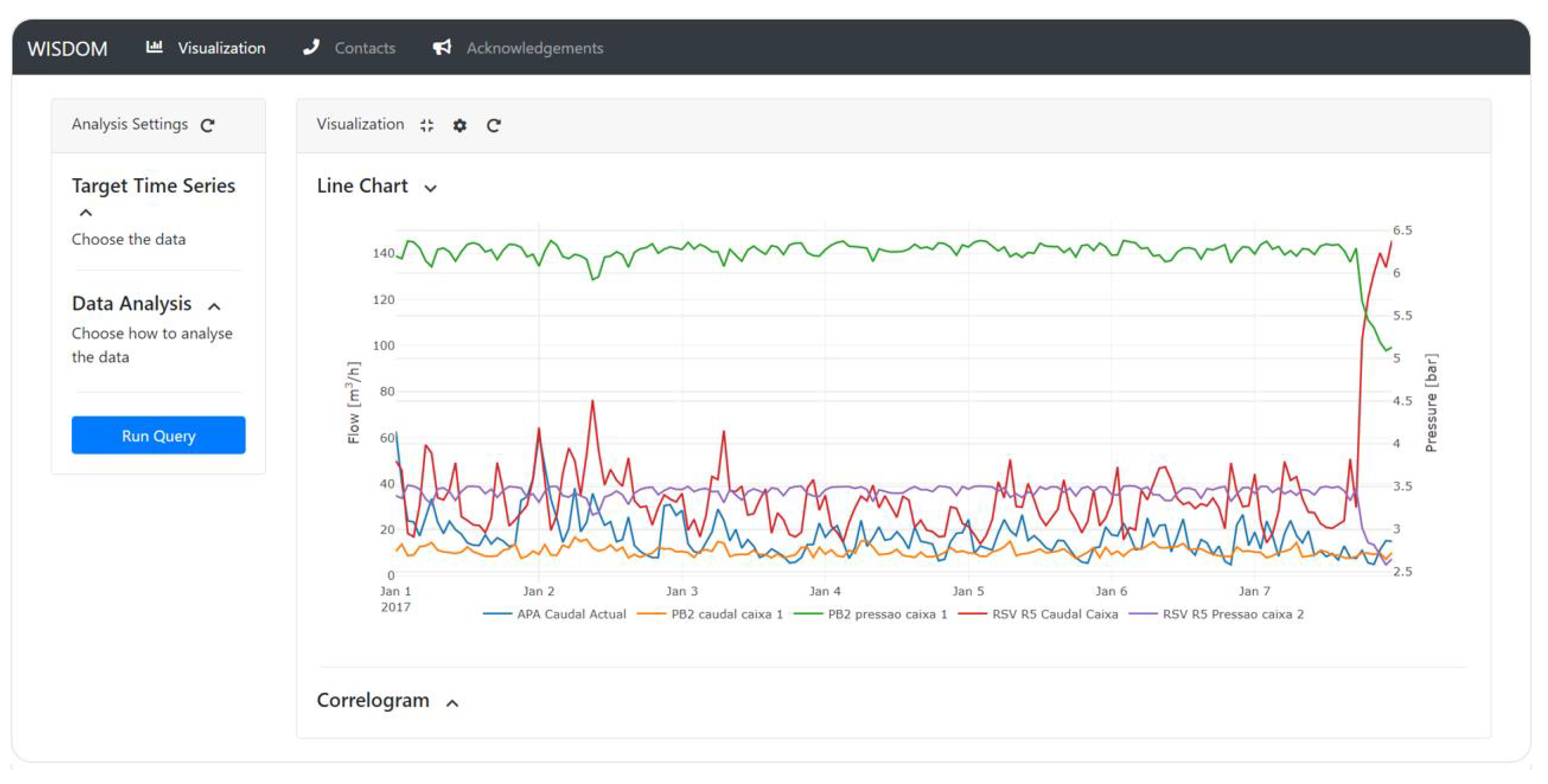
The tool consists in two major components, parameterization and visualization. The parameterization component, shown in Figure 2, allows users to select the (1) desirable WDN sensors and (2) analysis settings, respectively. In particular, the user can opt between different WDNs, types of sensors, periods of time, and correlations of interest.

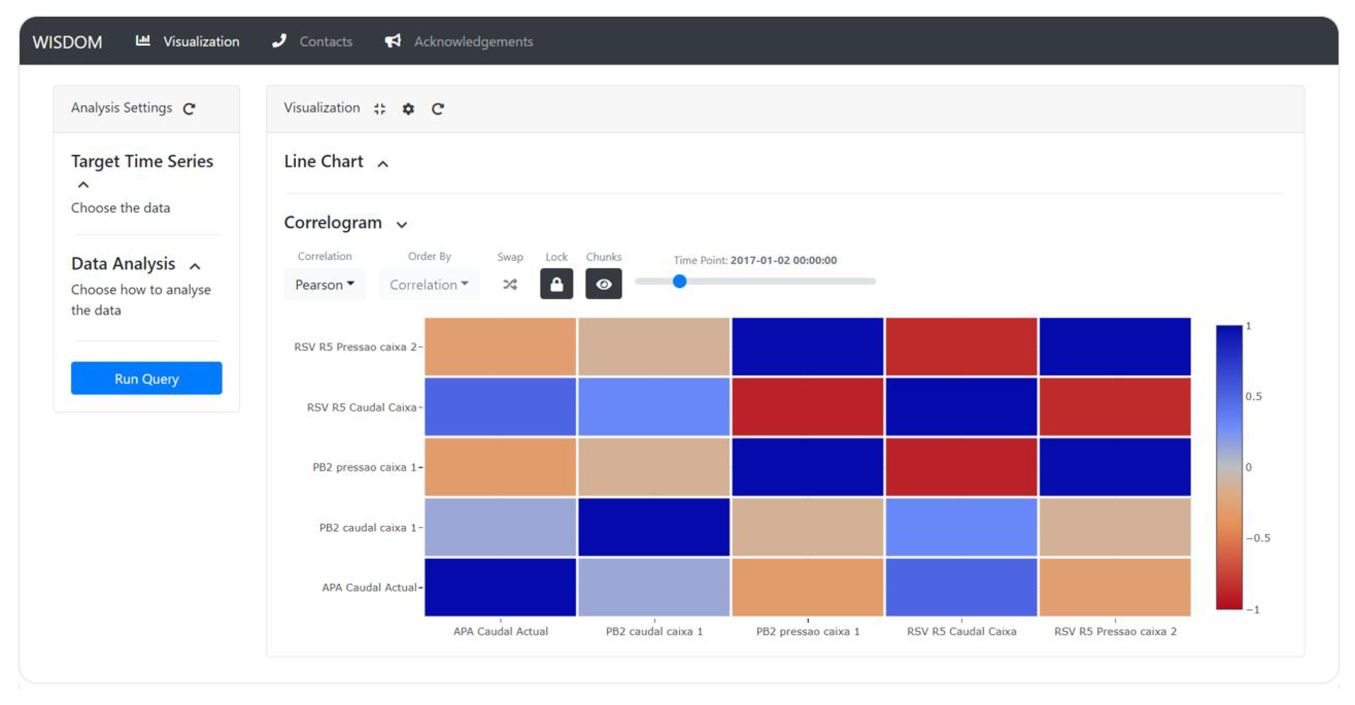
Regarding the visualization component, shown in Figure 3 and Figure 4, it offers a compound visualization the produced time series and an exploration of the correlations between the pairs of selected sensors. Spatiotemporal zoom-in-and-out facilities are further provided to the end user (Figure 3). In particular, the correlogram (Figure 4) offers sorting facilities by correlation value and geographical distances between sensor locations.

4. Results

Results gathered from the assessment of the proposed correlation-based principles aim at answering the formerly introduced research questions (Section 1). How leakage events affect pairwise correlations? How disruptions differ in real versus artificial settings? Which correlation coefficients are more sensitive to water leakages? How early can a leakage be detected? Which correlation-based parameters yield optimal sensitivity to true positive disruptions?

Accordingly, Section 4.1 introduces the Infraquinta’s case study, describing the properties of the target real and synthetic WDN settings. Section 4.2 assesses how pairwise correlations are disrupted in the presence of anomalous events. Section 4.3 shows how the correlation changes over time in respect to the starting moment of leakage occurrence. Section 4.4 assesses the sensitivity of correlation-based stances to different leakage sizes. Finally, Section 4.5 and Section 4.6 present how windowing and DCCA parameters affect the ability to assess disruptions to expected behavior.

4.1. Case Study: Infraquinta

The Infraquinta’s WDN is selected as our study case. Infraquinta serves Quinta do Lago, a tourist resort with extensive irrigation, large hotel units, and irregularities in the occupation of households. Therefore, Infraquinta’s WDN suffers from highly irregular consumption patterns, creating a challenging setting. The network is equipped with pressure and flowrate sensors.

4.1.1. Artificial WDN Data

The synthetic data was generated using an EPANET model of Infraquinta’s WDN, originating 18696 chunks of volumetric flowrate and pressure data. The flowrate data comprises data extracted from 7 network points, which location is equivalent to the location of flowrate sensors in the actual Infraquinta’s WDN (Figure 5). According to WU experts, the location of the existing pressure sensors is not suitable to identify most leakages. In this context, pressure data was extracted at 21 network points, where new pressure sensors could be added. The precise location of these sensors, together with the hydraulic model of Infraquinta’s WDN in EPANET, is provided as supplementary material at https://github.com/susanachambel/AnomalyDetectionInWaterDistributionNetworks (accessed on 8 September 2021). For simplification purposes, we refer to these 28 network points as sensors. Negative measurements, caused by the configuration of pipe directions in the EPANET model, can be found in data. The absolute value of measurements is therefore considered. Moreover, we found measurements very close to zero in flowrate sensors. Since there was no evidence of the existence of water flow in those situations, flowrate values below 1 ×${10}^{-3}$ are neglected. Each generated data chunk collects measurements along a typical day, and encompasses one leakage with a specific size and location. The leakages were generated using six leakage coefficients, namely, 0.05, 0.1, 0.5, 1.0, 1.5 and 2.0. The higher the coefficient, the larger the leakage is. In that way, our data covers all 3116 points of the network and six leakage sizes (18,696 = 3116 × 6). These leakages run for approximately 4 h and can happen anywhere in the chunk.

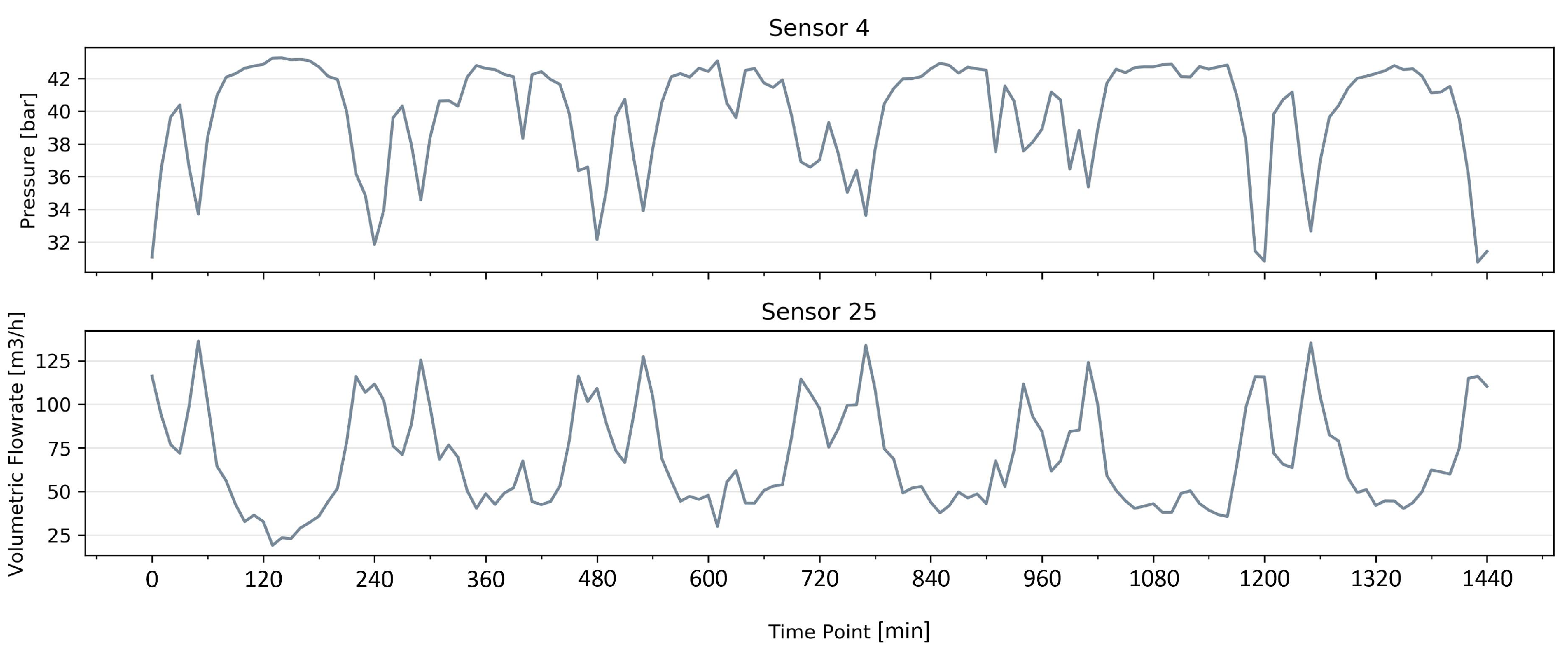
As expected, and shown in Figure 6, we can identify a clear seasonality in synthetic time series. Under these controlled conditions, disruptions in the network are more noticeable. We can also see that flowrate and pressure have well-established inverse correlation. Lastly,

Table 2. Statistics of synthetic pressure sensors 1 to 21 and flowrate sensors 22 to 28 from chunk 697.

	Pressure Sensors
	1	2	3	4	5	6	7	8	9	10	11	12	13	14
mean	23.13	39.43	60.10	39.91	27.37	40.71	34.01	43.92	48.14	37.59	48.80	33.30	48.33	43.53
std	1.26	1.09	0.56	3.23	0.08	1.33	1.97	2.15	2.03	2.08	1.97	1.97	1.98	2.83
min	19.43	36.21	58.47	30.78	27.07	35.57	26.82	35.51	40.92	29.35	41.52	26.12	41.11	35.82
25%	22.50	38.87	59.67	37.90	27.35	40.30	33.03	43.01	47.00	36.57	47.84	47.84	32.33	47.36
50%	23.54	39.79	60.30	41.17	27.39	41.12	34.20	44.12	48.34	37.64	48.97	48.97	33.50	48.54
75%	24.13	40.29	60.55	42.44	27.43	41.57	35.42	45.51	49.69	39.15	50.22	50.22	34.71	49.74
max	24.73	40.82	60.78	43.27	27.47	42.40	38.06	48.11	52.25	41.69	52.85	37.36	52.41	46.58
	Pressure Sensors							Volumetric Flowrate Sensors
	15	16	17	18	19	20	21	22	23	24	25	26	27	28
mean	42.76	30.66	43.80	32.56	34.80	25.94	25.99	8.63	87.68	177.68	68.68	28.96	0.00	0.24
std	4.66	4.59	4.53	0.61	0.49	0.77	0.45	5.50	18.30	35.93	28.46	11.69	0.00	1.32
min	30.84	19.30	32.66	30.66	33.14	23.28	24.48	1.66	40.77	97.86	19.15	9.00	0.00	0.00
25%	41.35	40.33	28.29	41.44	32.16	34.52	25.56	4.84	77.36	149.52	44.61	19.56	0.00	0.00
50%	44.66	44.04	31.98	45.09	32.59	34.85	26.20	7.06	89.02	177.39	62.03	26.43	0.00	0.00
75%	45.83	46.24	34.09	47.21	33.01	35.18	26.48	10.48	97.87	199.23	93.02	36.41	0.00	0.00
max	48.76	36.57	49.66	33.65	35.66	26.78	26.79	30.18	148.58	279.15	136.23	58.02	0.00	11.77

present the descriptive statistics of the produced synthetic data, offering a quantitative summary of the synthetic sensors from chunk 697, taken as an illustrative example.

4.1.2. Real WDN Data

The available real data were extracted from 7 volumetric flowrate and 6 pressure sensors, identified in

Table 3. Correspondence between the sensor location (Figure 5) and descriptors.

ID	Volumetric Flowrate Sensors	ID	Pressure Sensors
1	APA Caudal Atual	3	PB2 Pressão Caixa 1
2	PB2 Caudal Caixa 1	7	RSV R5 Pressão Caixa 2
6	RSV R5 Caudal Caixa	8	QV Sonda de Pressão
9	QV Caudal	11	RPR Pressão Pre
10	HC Caudal	13	RPR Pressão Grv
12	RPR Pre	15	APA Pressão
14	RPR Caudal Grv

, along the entire year of 2017. The WDN monitoring system has a granularity of approximately 60 s. Regarding leakages, out of 16 occurrences reported in 2017, we have complete information about 12, as shown in

Table 4. Reported leakages in 2017.

	Reported Time	Resolution Start	Resolution End
1	8 January 2017 08:30	8 January 2017 09:00	8 January 2017 14:00
2	7 February 2017 12:10	7 February 2017 12:15	7 February 2017 16:00
3	1 May 2017 04:20	1 May 2017 04:45	1 May 2017 10:35
4	7 May 2017 08:25	7 May 2017 09:15	7 May 2017 17:30
5	12 May 2017 11:15	12 May 2017 14:00	12 May 2017 16:20
6	13 June 2017 10:18	13 June 2017 11:03	13 June 2017 14:47
7	5 July 2017 03:00	5 July 2017 03:30	5 July 2017 10:45
8	9 September 2017 09:00	9 September 2017 09:15	9 September 2017 12:30
9	12 September 2017 09:35	12 September 2017 09:40	12 September 2017 11:30
10	1 December 2017 19:02	1 December 2017 19:30	1 December 2017 10:57
11	8 December 2017 16:40	8 December 2017 17:30	8 December 2017 20:30
12	12 November 2017 12:26	12 November 2017 13:40	12 November 2017 16:50

. It is also important to note that although we know the time leakages were reported, we do not know when they actually started nor its size. The produced measurements are recorded at irregular time steps. To estimate observations at a regular sampling (equally distant points), we applied a simple linear interpolation method.

Unlike the artificial WDN, all 13 sensors from Infraquinta are concentrated in three major areas, as shown in Figure 5. Consequently, the lack of sensor coverage may negatively impact the ability to detect leakages that do not occur between these areas.

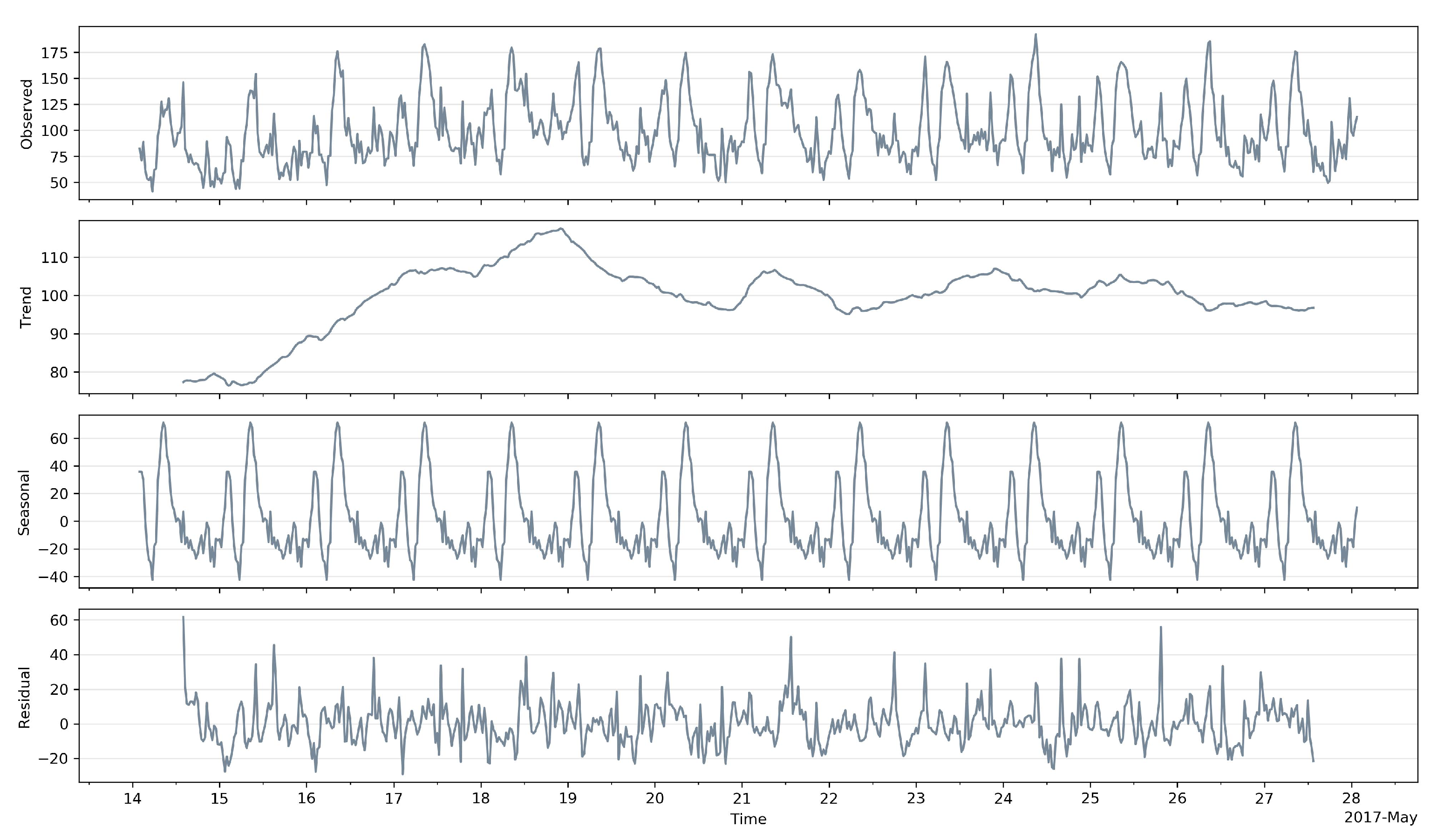
As expected, the time series from Infraquinta’s WDN are generally more complex than the synthetic ones, i.e., contain more noise, are vulnerable to network changes, and are exposed to irregular consumption patterns. All these factors make the analysis of time series more difficult. Figure 7 shows the decomposed components of two weeks of data from sensor 6 using an additive model. Although we are able to observe a clear seasonality, the time series contains large residuals and its trend does not convey enough information about what happened during these weeks. Lastly,

Table 5. Descriptive statistics of the real sensors from 15 to 28 May 2017.

	Pressure Sensors						Volumetric Flowrate Sensors
	3	7	8	11	13	15	1	2	6	9	10	12	14
mean	5.62	2.97	2.80	2.30	0.40	2.51	57.99	30.83	98.80	18.86	6.75	155.29	68.36
std	0.43	0.31	0.01	0.01	0.00	0.03	34.05	14.19	32.67	12.22	12.08	47.43	36.04
min	3.80	1.60	2.60	2.10	0.40	1.96	4.44	0.00	31.30	1.50	0.00	58.91	5.10
25%	5.40	2.80	2.80	2.30	0.40	2.50	28.94	20.70	75.59	9.20	0.00	119.21	38.30
50%	5.73	3.09	2.80	2.30	0.40	2.50	49.14	28.45	91.36	14.53	0.50	146.42	63.30
75%	5.93	3.20	2.80	2.30	0.40	2.50	83.70	39.41	119.80	27.20	7.10	186.86	94.30
max	6.30	3.50	3.03	2.40	0.40	2.70	159.80	78.46	208.30	56.20	51.40	331.95	186.37

presents the descriptive statistics of the real dataset. As sensors 8, 11, 13, and 15 appear to be almost constant during the whole year, they are not considered in the subsequent correlation-based analysis.

4.2. Correlation Analysis

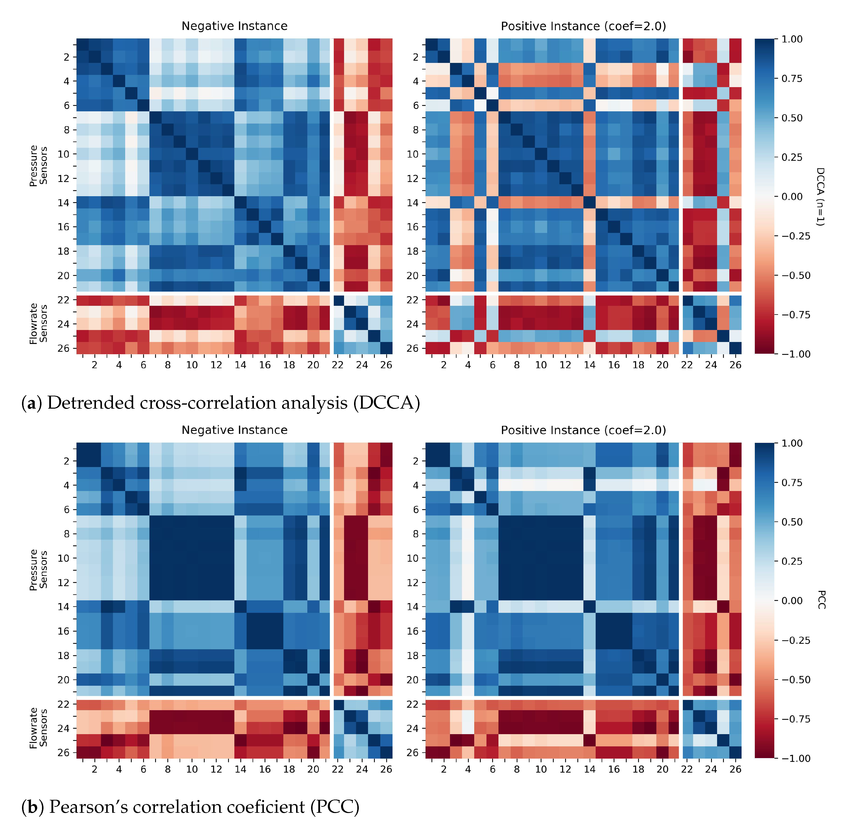
Figure 8 and Figure 9 assesses expectations and disruptions on the relationships between the WDN sensors accordance with the proposed feature construction step. To this end, one data instance can be visualized as a heatmap, where the presented values corresponds to a correlation coefficient (DCCA or PCC) between a pair of sensors, with the blue scale representing a positive correlation and the red scale representing an inverse correlation.

Regarding the artificial WDN, Figure 8 provides the correlogram of two synthetic instances, one negative (regular behavior) and on positive (burst occurrence) from the same chunk. Figure 8a uses DCCA as the correlation method, while Figure 8b uses PCC. When focusing on the regular behavior, we can observe that pairs of sensors of the same type are directly correlated, while pairs of different types are inversely correlated. DCCA and PCC also obtained similar coloring patterns, but PCC looks more robust against network disruptions since its correlations are stronger in both instances. Consequentially, the difference to the negative instance with PCC is less noticeable than with DCCA. Therefore, DCCA appears to be more sensitive to leakages in the synthetic setting and therefore contribute to better results in the subsequent leakage detection step than PCC.

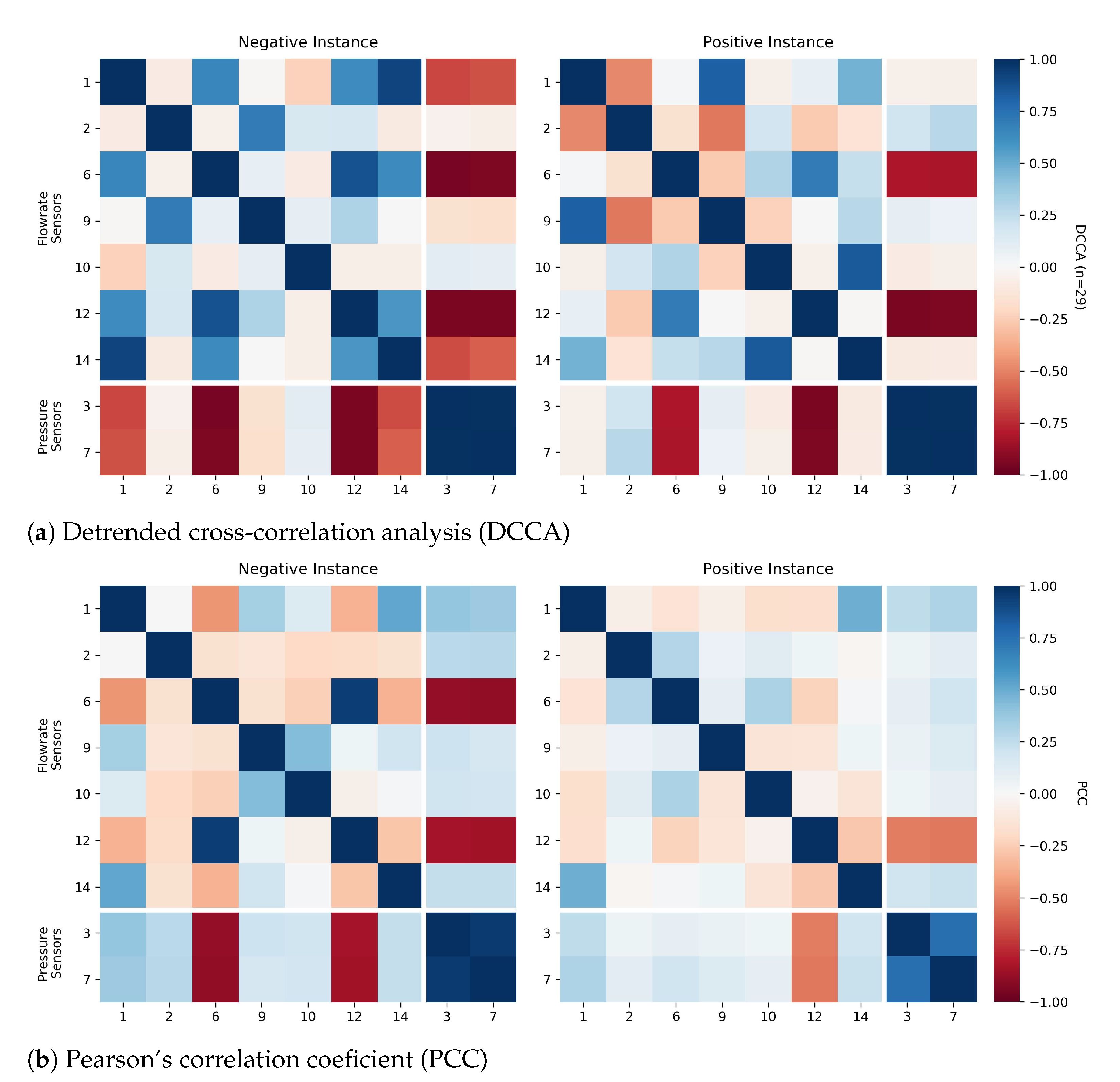
Considering real measurements produced by the 13 selected sensors in Infraquinta’s WDN, Figure 9 provide a comparable analysis. We can observe that, although the overall correlations are not as strong as in the synthetic dataset, we can clearly differentiate between regular and disrupted behavior. We also noticed that DCCA seems to consider most sensors of the same type as directly correlated and sensors of different types as inversely correlated. However, when using PCC, these correlations are not defined as clearly. When contrasting the negative and positive instances, while most correlations became weaker in PCC, some grew stronger in DCCA, highlighting the role of DCCA for describing anomalies.

Overall, Figure 8 and Figure 9 show preliminary empirical evidence in favor of the viability of the proposed correlation principle to detect and model disruptions to normal behavior.

4.3. Correlation over Time

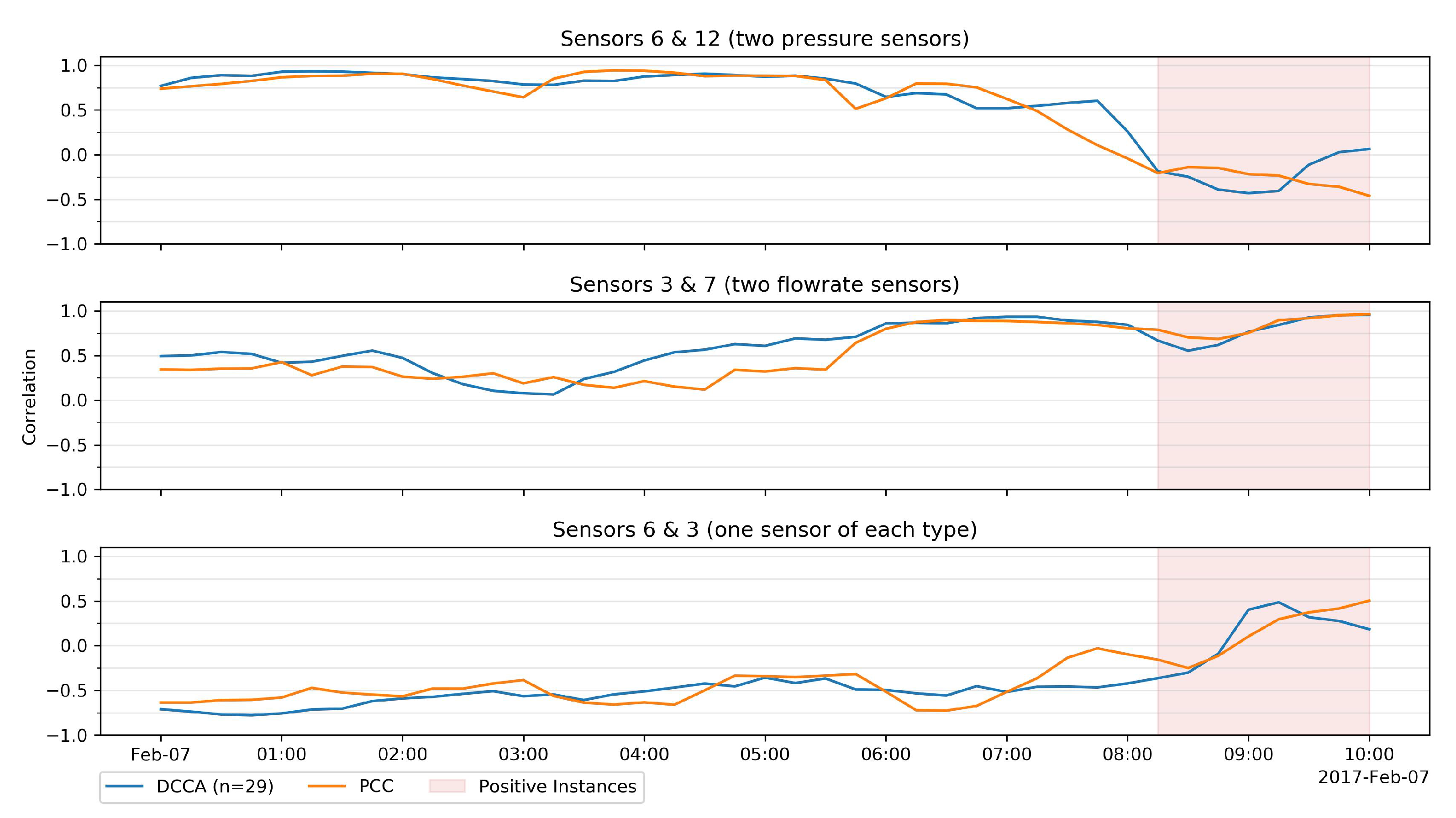
Another critical element to assess is how correlation evolves, especially before and during the leakage. To understand how the correlation changes over time in our synthetic setting, we created a sliding window that moves over the time series in intervals of 10 min. Figure 10 shows the DCCA and PCC over time in three selected pairs from the same chunk. Before the leakage, DCCA and PCC remained between 0.5 and 1, negative or positive, depending on whether the pair is positively or negatively correlated. Moments after the leakage occurred, the correlations got weaker and closer to zero until they started getting stronger again. We can infer that this point corresponds to when the time window includes more leakage points than non-leakage points. Figure 10 also shows that DCCA oscillates a lot more than PCC, causing the impact of the leakage to be more apparent in DCCA.

Regarding the real setting, shown in Figure 11, the behavior of DCCA and PCC is very similar. Both methods are more unstable before the leakage, which is probably an indication that these methods cannot accurately quantify the correlation value between time series due to the large volume of noise present. Although the differences between the negative and the positive instances are not as striking as in the synthetic dataset, we can still notice a subtle change after the leakage. Since PCC has not outperformed DCCA so far, and to make the analysis less exhaustive, the next sections of this chapter will only include the results obtained through DCCA.

4.4. Correlation in Small Leakages

For the experiments in the synthetic setting, we have been using a leakage coefficient of $2.0$, which makes it a medium-sized leakage. However, since smaller leakages can also happen in WDNs, it is vital to understand how DCCA responds to them. Therefore, Figure 12 compares the disruption on the DCCA values for six different leakage coefficients.

As we can see, the DCCA value for coefficients below $0.5$ is very close to the value obtained without a leakage. However, the correlation weakens considerably for leakages above $0.5$. As expected, larger leakages seem to cause a higher disruption in DCCA than the smaller ones. Consequently, smaller leakages may be more difficult to detect than larger ones. Although we cannot perform this analysis for the real setting because we do not have information about the leakage sizes, we hypothesize from the gathered results that the disruptions caused by smaller leakages ($coef\le 0.1)$ may be hard to detect.

4.5. Time Window Size

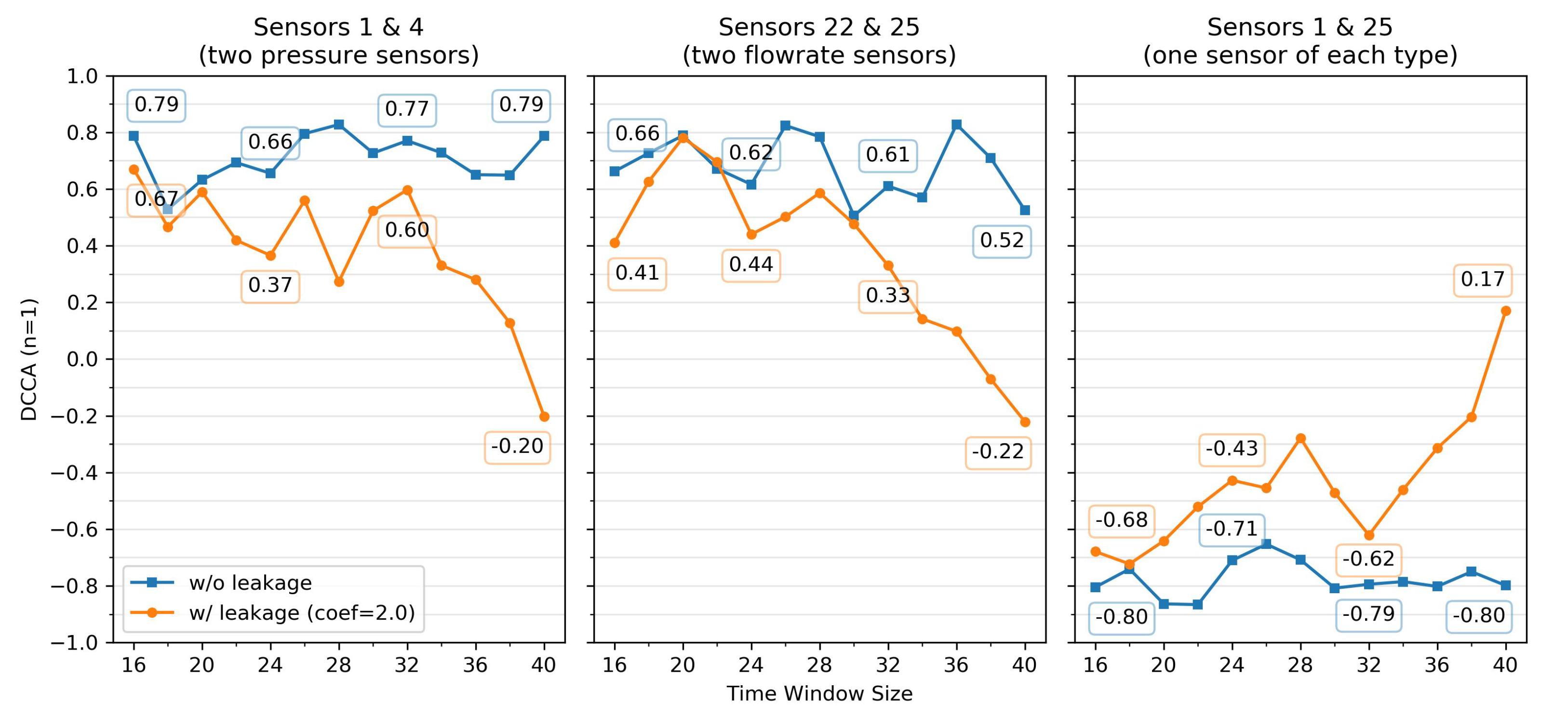
Until now, we have been using a time window of 40 time points for the synthetic setting. Figure 13 helps us understand how DCCA is affected by different time windows between 16 and 40 time points. Through the analysis of the positive and the negative instances, we can see that the difference between them seems considerably random until 32 time points. Around that period, DCCA values start diverging, peaking at 40 time points. One possible explanation is that DCCA could not accurately identify the degree of correlation with less than 32 points. Lastly, since the 40 time point window showed the largest correlation difference between instances, it may contribute to better results in the classification step than the others.

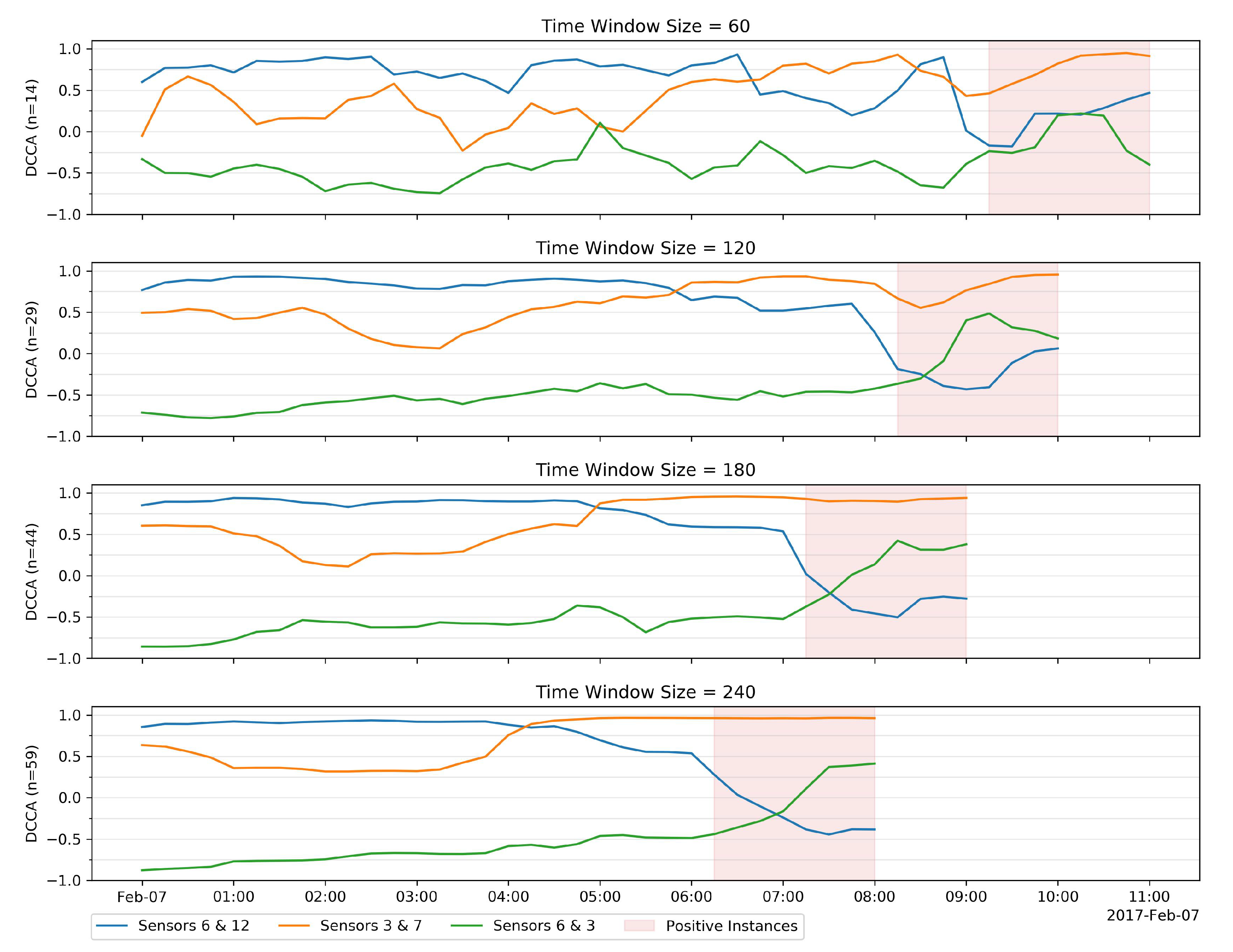
Regarding the real setting, we have been using a time window of 120 min. Figure 14 shows how DCCA is affected by four different time windows between 60 and 240 min. Although the 60 min time window fluctuates a lot more than the others, all of them behave similarly over time. We can also see that the smaller its size, the greater its fluctuation. Focusing on the time window of 60 min, we can see that too much variation disguises the leakage. Contrarily, 240 min causes so much stability that the correlation between sensors 3 and 7 does not change during the leakage. Lastly, the time window of 120 min seems to be very balanced, i.e., it does not fluctuate as much as one of 60 min but varies enough to let us still notice the difference between negative and positive instances.

4.6. DCCA Parameterization

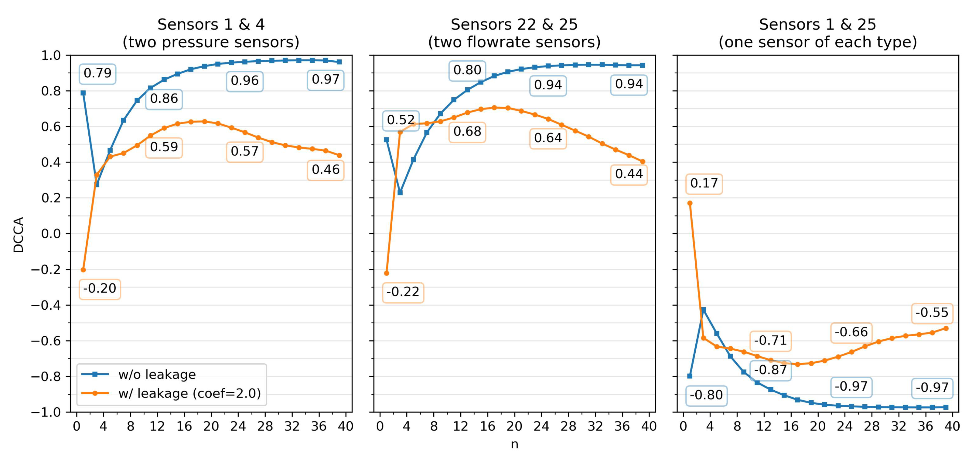
As introduced in Section 2, DCCA is dependent on the parameterized size of the overlapping boxes. As such, it is important to assess its impact. Considering that $1\le n<N$, where N is the size of the time window, Figure 15 plots the DCCA for n values between 1 and 39 points for the synthetic setting. We can observe that when $n=1$, the difference between the DCCA values for the negative and the positive instances reaches its peak. For $n>1$, the difference between instances slowly grows until $n=39$, its best value after $n=1$. Peak values may contribute to support the classification of anomalous behavior.

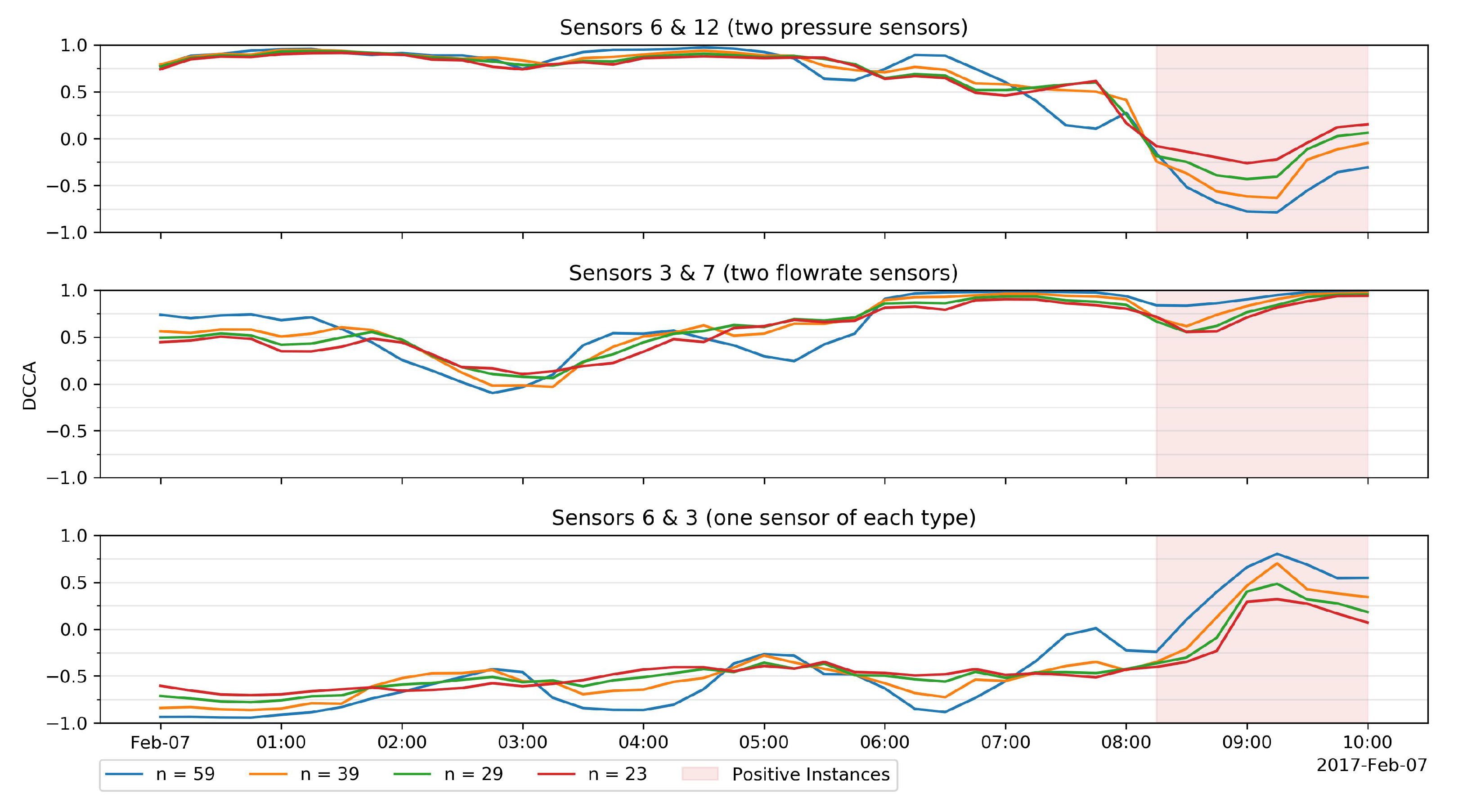
To understand how n affects DCCA in the real setting, we chose four different boxes’ sizes, corresponding to 1/2, 1/3, 1/4 and 1/5 of the size of the target time window. Figure 16 shows how the correlation of each pair is affected by each n value. Although all four values of n seem to follow the same pattern, $n=59$ stands out from the others as it fluctuates more between negative and positive instances.

5. Discussion and Concluding Remarks

This work proposes a shift on the current way of modeling anomalous events in WDNs by placing the emphasis on the analysis of time-varying pairwise correlations between sensors spatially distributed along a network. Experiments conducted in a controlled environment and in a real WDN with highly irregular consumption patterns confirm the relevance of the introduced principles for leakage detection.

In particular, we show that leakages of varying magnitudes cause unexpected disruptions on the sensor relationships at all levels–between pressure sensors, flowrate sensors, and between pressure-flowarate paired sensors. DCCA generally provided better results against classic PCC coefficients, suggesting the relevance of temporal cross-correlation stances. In addition, we observed that increasing the size of the sliding window does not always increase predictive accuracy and might camouflage the leakages. Specifically, a 60 min window provided better results than a 180 and a 240 min window, and experiments further showed that the maximum disruption of the correlation happens when the middle of the time window aligns with the beginning of the leakage, suggesting that small-to-medium sized bursts can be detected within 15 to 30 min.

The proposed correlation-based feature space is able to capture leakage perturbations in a large WDN with sparse sensor coverage, attesting the validity of the proposed contributions under suboptimal sensor placement. In this context, the assessment of the proposed methodology in WDNs with broader sensor coverage is identified as an important prospective direction to assess the generalization of the collected observations and acquire a more comprehensive understanding on how correlation disruptions vary with sensor distance and density.

We further highlight three major additional directions. First, a comprehensive comparison of predictive models for leakage detection from pairwise correlations. Given the generally low number of annotated leakages, special attention needs to be paid to the incorporation of class balancing principles along the learning process. Second, the discrimination between anomalies and ongoing changes in the network dynamics caused, for instance, by interventions. In particular, the proposed approach can be extended in order to dynamically update the learnt correlation-based expectations in the presence of events that change the network topology, such as network extensions and valve closures-or-openings. Finally, an assessment of the relevance of the proposed methodology for isolating the localization of bursts from the most disrupted sensor pairs, in accordance with the introduced principles (Section 3.2).

The proposed correlation-based views open an important door in water research as their applicability traverses many applications of interest. The underlying pairing principle can be used to guide the placement of new volumetric flowrate and pressure sensors, while the analysis of disruptions can be further pursued to dynamically detect changes in the status of active hydraulic elements, fraud events, and background leakages.

References

- Mays, L.W. Water Distribution System Handbook; McGraw-Hill Education: New York, NY, USA, 2000. [Google Scholar]
- Colombo, A.; Karney, B. Energy and Costs of Leaky Pipes: Toward Comprehensive Picture. J. Water Resour. Plan. Manag. 2002, 128, 441–450. [Google Scholar] [CrossRef] [Green Version]
- Li, R.; Huang, H.; Xin, K.; Tao, T. A review of methods for burst/leakage detection and location in water distribution systems. Water Sci. Technol. Water Supply 2015, 15, 429–441. [Google Scholar] [CrossRef]
- Zhou, M.; Pan, Z.; Liu, Y.; Zhang, Q.; Cai, Y.; Pan, H. Leak Detection and Location Based on ISLMD and CNN in a Pipeline. IEEE Access 2019, 7, 30457–30464. [Google Scholar] [CrossRef]
- Hu, P.; Tong, J.; Wang, J.; Yang, Y.; de Oliveira Turci, L. A hybrid model based on CNN and Bi-LSTM for urban water demand prediction. In Proceedings of the 2019 IEEE Congress on Evolutionary Computation (CEC), Wellington, New Zealand, 10–13 June 2019; pp. 1088–1094. [Google Scholar]
- Mounce, S.; Boxall, J.; Machell, J. An artificial neural network/fuzzy logic system for DMA flow meter data analysis providing burst identification and size estimation. In Water Management Challenges in Global Change; Taylor & Francis: Abingdon, UK, 2007; pp. 313–320. [Google Scholar]
- Mounce, S.; Boxall, J.; Machell, J. Online application of ANN and fuzzy logic system for burst detection. In Water Distribution Systems Analysis; American Society of Civil Engineers: Reston, VA, USA, 2008; pp. 1–12. [Google Scholar]
- Puust, R.; Kapelan, Z.; Savic, D.; Koppel, T. A review of methods for leakage management in pipe networks. Urban Water J. 2010, 7, 25–45. [Google Scholar] [CrossRef]
- Aksela, K.; Aksela, M.; Vahala, R. Leakage detection in a real distribution network using a SOM. Urban Water J. 2009, 6, 279–289. [Google Scholar] [CrossRef]
- Mounce, S.R.; Mounce, R.B.; Boxall, J.B. Novelty detection for time series data analysis in water distribution systems using support vector machines. J. Hydroinformatics 2011, 13, 672–686. [Google Scholar] [CrossRef]
- Mashford, J.; De Silva, D.; Marney, D.; Burn, S. An approach to leak detection in pipe networks using analysis of monitored pressure values by support vector machine. In Proceedings of the 2009 Third International Conference on Network and System Security, Gold Coast, QLD, Australia, 19–21 October 2009; pp. 534–539. [Google Scholar]
- Mounce, S.R.; Machell, J. Burst detection using hydraulic data from water distribution systems with artificial neural networks. Urban Water J. 2006, 3, 21–31. [Google Scholar] [CrossRef]
- Mounce, S.R.; Khan, A.; Wood, A.S.; Day, A.J.; Widdop, P.D.; Machell, J. Sensor-fusion of hydraulic data for burst detection and location in a treated water distribution system. Inf. Fusion 2003, 4, 217–229. [Google Scholar] [CrossRef]
- Jalalkamali, A.; Jalalkamali, N. Application of hybrid neural modeling and radial basis function neural network to estimate leakage rate in water distribution network. World Appl. Sci. J. 2011, 15, 407–414. [Google Scholar]
- Guyon, I.; Gunn, S.; Nikravesh, M.; Zadeh, L.A. Feature Extraction: Foundations and Applications; Springer: Berlin/Heidelberg, Germany, 2008; Volume 207. [Google Scholar]
- Valizadeh, S.; Moshiri, B.; Salahshoor, K. Leak detection in transportation pipelines using feature extraction and KNN classification. In Pipelines 2009: Infrastructure’s Hidden Assets; American Society of Civil Engineers: Reston, VA, USA, 2009; pp. 580–589. [Google Scholar]
- Cembrano, G.; Wells, G.; Quevedo, J.; Pérez, R.; Argelaguet, R. Optimal control of a water distribution network in a supervisory control system. Control Eng. Pract. 2000, 8, 1177–1188. [Google Scholar] [CrossRef] [Green Version]
- Farley, M.; Trow, S. Losses in Water Distribution Networks; IWA Publishing: London, UK, 2003. [Google Scholar]
- Farley, M.; Water, S.; Supply, W.; Council, S.C.; World Health Organization. Leakage Management and Control: A Best Practice Training Manual; Technical Report; World Health Organization: Geneva, Switzerland, 2001. [Google Scholar]
- Araujo, L.; Ramos, H.; Coelho, S. Pressure control for leakage minimisation in water distribution systems management. Water Resour. Manag. 2006, 20, 133–149. [Google Scholar] [CrossRef]
- Rossman, L.A. EPANET 2: Users Manual; US Environmental Protection Agency, Office of Research and Development: Washington, DC, USA, 2000.
- Sonaje, N.P.; Joshi, M.G. A review of modeling and application of water distribution networks (WDN) softwares. Int. J. Techical Res. Appl. 2015, 3, 174–178. [Google Scholar]
- Dagum, E.B.; Bianconcini, S. Seasonal Adjustment Methods and Real Time Trend-Cycle Estimation; Springer: Berlin/Heidelberg, Germany, 2016. [Google Scholar]
- Kruskal, J.B. Multidimensional scaling by optimizing goodness of fit to a nonmetric hypothesis. Psychometrika 1964, 29, 1–27. [Google Scholar] [CrossRef]
- Müller, M. Dynamic time warping. In Information Retrieval for Music and Motion. Springer: Berlin/Heidelberg, Germany, 2007; pp. 69–84. [Google Scholar]
- Senin, P. Dynamic time warping algorithm review. Inf. Comput. Sci. Dep. Univ. Hawaii Manoa Honolulu USA 2008, 855, 40. [Google Scholar]
- Keogh, E.J.; Pazzani, M.J. Derivative dynamic time warping. In Proceedings of the 2001 SIAM International Conference on Data Mining, Chicago, IL, USA, 5–7 April 2001; pp. 1–11. [Google Scholar]
- Keogh, E.; Ratanamahatana, C.A. Exact indexing of dynamic time warping. Knowl. Inf. Syst. 2005, 7, 358–386. [Google Scholar] [CrossRef]
- Serra, J.; Arcos, J.L. An empirical evaluation of similarity measures for time series classification. Knowl.-Based Syst. 2014, 67, 305–314. [Google Scholar] [CrossRef] [Green Version]
- Levenshtein, V.I. Binary codes capable of correcting deletions, insertions, and reversals. In Soviet Physics Doklady; American Institute of Physics: College Park, MD, USA, 1966; Volume 10, pp. 707–710. [Google Scholar]
- Chen, L.; Özsu, M.T.; Oria, V. Robust and fast similarity search for moving object trajectories. In Proceedings of the 2005 ACM SIGMOD International Conference on Management of Data, Baltimore, MD, USA, 14–16 June 2005; pp. 491–502. [Google Scholar]
- Marteau, P.F. Time warp edit distance with stiffness adjustment for time series matching. IEEE Trans. Pattern Anal. Mach. Intell. 2008, 31, 306–318. [Google Scholar] [CrossRef] [PubMed] [Green Version]
- Lhermitte, S.; Verbesselt, J.; Verstraeten, W.W.; Coppin, P. A comparison of time series similarity measures for classification and change detection of ecosystem dynamics. Remote Sens. Environ. 2011, 115, 3129–3152. [Google Scholar] [CrossRef]
- Bermudez-Edo, M.; Barnaghi, P.; Moessner, K. Analysing real world data streams with spatio-temporal correlations: Entropy vs. Pearson correlation. Autom. Constr. 2018, 88, 87–100. [Google Scholar] [CrossRef]
- de Winter, J.C.; Gosling, S.D.; Potter, J. Comparing the Pearson and Spearman correlation coefficients across distributions and sample sizes: A tutorial using simulations and empirical data. Psychol. Methods 2016, 21, 273. [Google Scholar] [CrossRef] [PubMed]
- Laih, Y.W. Measuring rank correlation coefficients between financial time series: A GARCH-copula based sequence alignment algorithm. Eur. J. Oper. Res. 2014, 232, 375–382. [Google Scholar] [CrossRef]
- Podobnik, B.; Stanley, H.E. Detrended cross-correlation analysis: A new method for analyzing two nonstationary time series. Phys. Rev. Lett. 2008, 100, 084102. [Google Scholar] [CrossRef] [PubMed] [Green Version]
- Horvatic, D.; Stanley, H.E.; Podobnik, B. Detrended cross-correlation analysis for non-stationary time series with periodic trends. EPL Europhys. Lett. 2011, 94, 18007. [Google Scholar] [CrossRef] [Green Version]
- Zebende, G.F. DCCA cross-correlation coefficient: Quantifying level of cross-correlation. Phys. A Stat. Mech. Its Appl. 2011, 390, 614–618. [Google Scholar] [CrossRef]
- Kruskal, W.H.; Wallis, W.A. Use of ranks in one-criterion variance analysis. J. Am. Stat. Assoc. 1952, 47, 583–621. [Google Scholar] [CrossRef]
Figure 1.
Infraquinta’s WDN, serving Quinta do Lago, a large touristic urbanization in Algarve, Portugal.
Figure 2.
Decision support tool: parameterization component.
Figure 3.
Decision support tool: series visualization with sensor and temporal selection facilities.
Figure 4.
Decision support tool: correlogram section with coefficient and spatial sorting and zooming facilities.
Figure 5.
Overview of the real sensors’ location in Infraquinta’s WDN.
Figure 6.
Synthetic time series of sensors 4 and 25 from chunk 697.
Figure 7.
Additive decomposition of flowrate sensor 6 from 15 to 28 May 2017.
Figure 8.
Correlograms of two synthetic instances from chunk 702 using a window of 40 time points.
Figure 9.
Correlograms of two real instances in 7 February 2017, using a 120 min time window. Negative instance occurs between 10:00 and 12:00, while the positive one between 14:45 and 16:45.
Figure 10.
DCCA and PCC over time in three selected sensor pairs from chunk 702 using a time window of 40 time points.
Figure 11.
DCCA and PCC over time in three selected pairs from 7 February 2017, using a time window of 120 min.
Figure 12.
DCCA variation with the leakage coefficient in three selected pairs from chunk 702 using a time window of 40 time points.
Figure 13.
Impact of time window size on DCCA in three selected pairs from chunk 702.
Figure 14.
Impact of time window size on DCCA in three selected pairs from from 7 February 2017.
Figure 15.
Impact of parameter n on DCCA in three selected pairs from chunk 702 using a time window of 40 time points.
Figure 16.
Impact of parameter n on DCCA in three selected pairs from 7 February 2017, using a time window of 120 min.