
Data- and Model-Based Discharge Hindcasting over a Subtropical River Basin


1
Department of Civil and Environmental Engineering, University of Texas at San Antonio, San Antonio, TX 78249, USA
2
CPS Energy, 500 McCullough Ave, San Antonio, TX 78215, USA
*
Author to whom correspondence should be addressed.
Water 2021, 13(18), 2560; https://doi.org/10.3390/w13182560
Submission received: 24 August 2021
/
Revised: 14 September 2021
/
Accepted: 16 September 2021
/
Published: 17 September 2021
(This article belongs to the Special Issue Catchment-Scale Solutions in the Context of Climate Change)
Abstract
:This study aims to evaluate the performance of the Soil and Water Assessment Tool (SWAT), a simple Auto-Regressive with eXogenous input (ARX) model, and a gene expression programming (GEP)-based model in one-day-ahead discharge prediction for the upper Kentucky River Basin. Calibration of the models were carried out for the period of 2002–2005 using daily flow at a stream gauging station unaffected by the flow regulation. Validation of the calibrated models were executed for the period of 2008–2010 at the same gauging station along with another station 88 km downstream. GEP provided the best calibration (coefficient of determination (R) value 0.94 and Nash-Sutcliffe Efficiency (NSE) value of 0.88) and validation (R values of 0.93 and 0.93, NSE values of 0.87 and 0.87, respectively) results at the two gauging stations. While SWAT performed reasonably well in calibration (R value 0.85 and NSE value 0.72), its performance somewhat degraded in validation (R values of 0.85 and 0.82, NSE values of 0.65 and 0.65, for the two stations). ARX performed very well in calibration (R value 0.92, NSE value 0.82) and reasonably well in validation (R values of 0.88 and 0.92, NSE values of 0.76 and 0.85) at the two stations. Research results suggest that sophisticated hydrological models could be outperformed by simple data-driven models and GEP has the advantage to generate functional relationships that allows investigation of the complex nonlinear interrelationships among the input variables.
1. Introduction
The availability of water at the watershed or basin scales in addition to the spatial and temporal distribution of water are largely affected by climatic and topographic factors [1]. Soil, land cover, and land use characteristics are also considered when studying the movement and exchange of water [2]. The recent development of robust hydrologic models and significant advancement in the processing power of computers [3] allow modelers to take these factors into account when trying to solve the complexity of hydrological processes. These models, often embedded within decision support tools, are especially necessary when complete information and observed data on discharge, inflow, climate, soil moisture, or other related factors of a basin are limited [4]. Changes in water budget and fluxes within a watershed can be studied based on the estimation and simulation of the models. Several popular conceptual and physically based watershed models have been used for discharge and water quality modeling in the last three decades including CREAMS (Chemical Runoff and Erosion from Agricultural Management Systems) [5], PRMS (Precipitation Runoff Modeling System) [6], HSPF (Hydrologic Simulation Program—Fortran) [7], SWAT (Soil and Water Assessment Tool) [8], and SWBM (Spatial Water Budget Model) [9]. These models are computationally effective and require relatively small time steps to produce outputs through simulations [10]. Among these models, SWAT can analyze how the changes in land use and land cover impact the runoff and water quality in addition to its ability to quantify the hydrological responses to the variation of hydrometeorological conditions, making it reliable and popular. Models equipped with data-driven techniques, on the other hand, have been found to be highly efficient to analyze the nonlinear and non-stationary relationship of rainfall and runoff [11]. For example, models which used Genetic Programming (GP) and Artificial Neural Network (ANN) in analyzing the evapotranspiration process outperformed the Penman-Monteith (PM) method [12]. Linear genetic programming (LGP) model equipped with ensemble empirical mode decomposition (EEMD) and self-organizing map (SOM) outperformed the ANN model in analyzing the rainfall–runoff relationship in Kentucky River [13]. Another study used GEP to model streamflow and the performances of GEP and feed forward back propagation ANNs were similar [14].
In this study, SWAT, Auto-Regressive with eXogenous input (ARX), and GEP models were selected to predict the daily river discharge of the upper Kentucky River. The Kentucky River supplies water for daily uses of the citizens living in the basin and plays an important role in improving the socio-economic condition of Kentucky State. However, the water quantity and quality of Kentucky River were adversely impacted by droughts and flooding caused by mountaintop removal and mining [15]. A system of 14 locks and dams were built, operated, and maintained in the last two centuries to ensure water supply sustainability and mitigate drought impacts [16]. Profound grasp of the hydrological regime of Kentucky River can support long-term water resources management. A comprehensive physically-based model like SWAT or data-driven models such as ARX or GEP could be helpful to forecast the runoff and the river discharge with acceptable accuracy and could be used to support long-term water resources management. The main objective of this study is to test the performances and suitability of SWAT, ARX, and GEP models in forecasting the daily discharge of the upper Kentucky River for a 3-year period (hindcasting) by calibrating the models and then spatially and temporally validating the performances of the calibrated models.
2. Simulation Methodology
2.1. Study Area
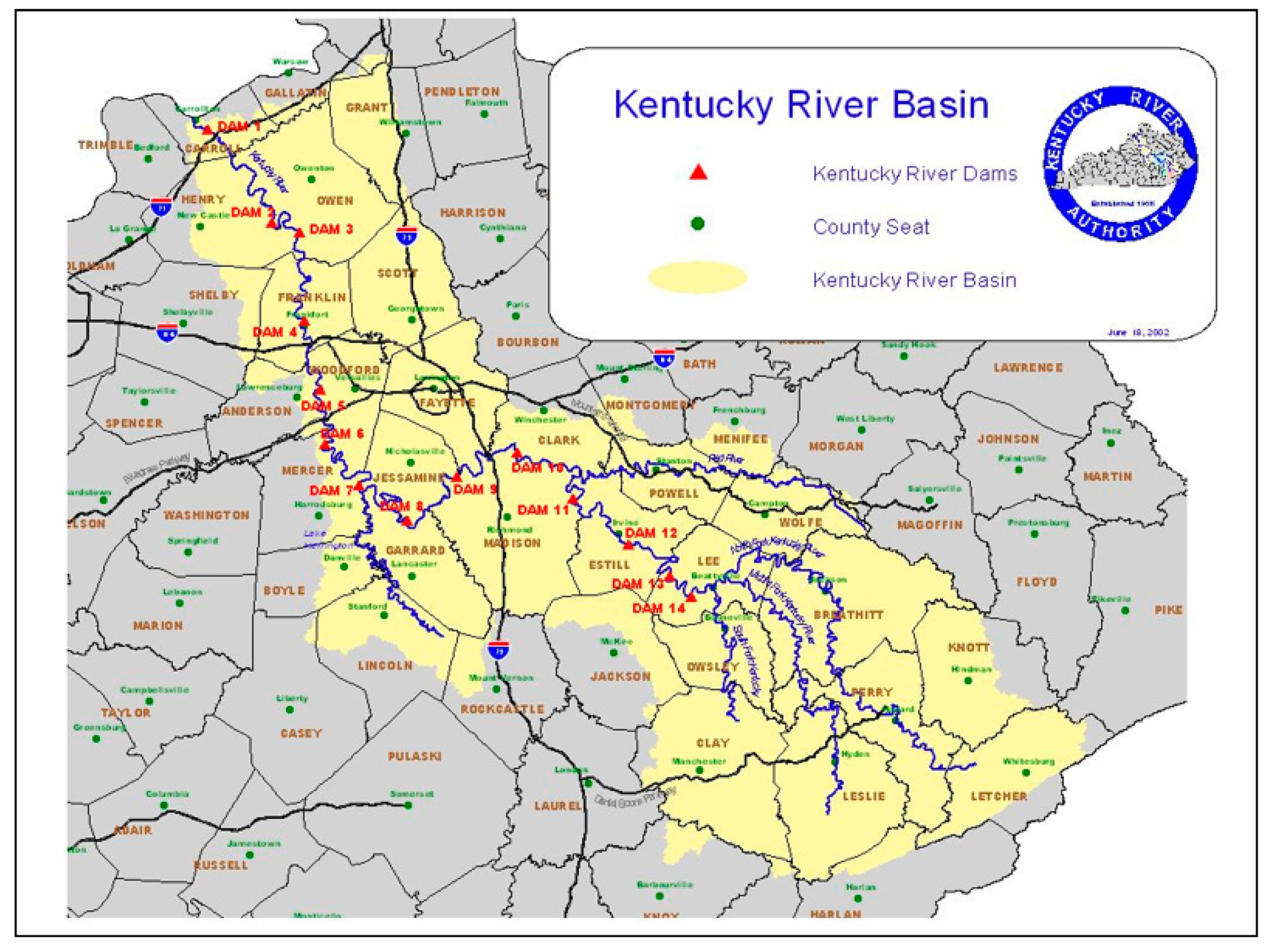
The Kentucky River Basin covers 42 counties of the state of Kentucky, with a total area of about 18,000 km2. The major tributaries of Kentucky River include Red River, Eagle Creek, North Fork Kentucky River, Elkhorn Creek, Middle Fork Kentucky River, Dix River, and the South Fork Kentucky River (Figure 1). The length of the main stem of Kentucky River is 418 km with a dense network of tributaries and streams that feed the river with a total length of approximately 25,700 km. The elevation of Kentucky River Basin ranges from 243 m to 305 m above the mean sea level with an average slope 0.13 m/km. The mean annual rainfall within the basin is approximately 1168 mm [17]. Climate in the basin is moist-continental and the average annual temperature is 13 °C. The basin experiences the minimum daily temperature in January and February (about −4 °C) while July and August bring the maximum daily temperature (about 31 °C) [18]. A system consisting of 14 locks and dams (LDs) was built on Kentucky River from downstream to upstream during the periods of 1836–1842 (LD 1–5), 1888–1891 (LD 6), 1896–1897 (LD 7), 1898–1900 (LD 8), 1901–1903 (LD 9), 1902–1905 (LD 10), 1904–1906 (LD 11), 1907–1910 (LD 12), 1909–1915 (LD 13), and 1911–1917 (LD 14) [19]. The older LDs (built in 19th century) were primarily built as timber crib and stone masonry structures and the relatively newer LDs (built in 20th century) were primarily built out of concrete. While most of the LDs (LD 5–14) are out of operation at present and have been sealed with concrete barriers, four LDs (LD 1–4) are still in operation (located within 65 river miles above mouth) and have been rebuilt and repaired over time [20].
To avoid the impact of the LDs on the natural flow of Kentucky River, a point that drains the North Fork Kentucky watershed, the Middle Fork Kentucky watershed, and the South Fork Kentucky watershed where none of the LDs is present is selected for calibration of the hydrologic model. This point drains about 6888 km2 and has its discharge recorded daily by USGS 03282000 stream gauge, which is located just upstream of LD 14 at Heidelberg, Kentucky. However, in addition to the natural flow sub-basin, the validation of the hydrologic model and other models was also performed on upper Kentucky River Basin (Figure 1). The outlet of upper Kentucky River is located just upstream from LD 10, near Winchester, Kentucky at the USGS 03284000 stream gauge. With the presence of four dams LD 11–14 within the upper Kentucky River, the outlet discharge is affected, to some extent, by operation of the LDs.
2.2. Models
2.2.1. The SWAT Model
SWAT is a semi-distributed, physically based eco-hydrologic model that is based on dividing the basin being modeled into smaller sub-basins, each of which can be divided into smaller hydrologic response units (HRUs) incorporating unique combinations of soil type, ground slope, and land use [22,23]. The SWAT is being widely used in hydrologic and ecologic simulations over basins of different scales in the US and other regions of a wide range of climatic and geologic conditions [24,25,26]. SWAT simulates the following water balance equation in its hydrologic simulation:
where SW represents soil water content minus the 15-bar pressure water content; t represents the time in days; R represents the amount of precipitation on day (mm); Q represents the daily runoff (mm); ET represents the daily evapotranspiration on day (mm); P represents the percolation on day (mm); and QR represents the return flow on day (mm). The SWAT model can select from a variety of methods in the calculation of surface runoff, channel flow, evapotranspiration, and other watershed dynamics before running a simulation. The model thus incorporates a myriad of parameters. Arnold and Srinivasan [22] described all the parameters of the water balance equation and its components in detail.
2.2.2. The ARX Model
The ARX (Auto-Regressive with eXogenous input) is a computationally and conceptually simple linear regression-based representation of a random process output variable that linearly depends on its own previous values, the previous values of another external (exogenous) variable, and on a stochastic term. ARX has been widely used to model the dynamic response of a system to exogenous factors in different fields including hydrology, agriculture, chemical engineering, medicine, biological science, and energy economics [27,28]. An autoregressive model has a physical hydrologic basis in baseflow recession theory because the lag-1 serial correlation coefficient of the model is equivalent to the widely used hydrograph recession constant [29,30]. The objective in this study is to develop and implement an ARX model at LD10 and LD14 of Kentucky River Basin that can forecast the discharge one-step ahead. The following equation represents the ARX model:
where e(t) refers to the noise (assumed to be Gaussian); ana and bnb represents the model parameters; the order of the polynomials of the output A(q) and the input B(q) are represented by na and nb, respectively; and the time delay between y(t) and u(t) is represented by nk. Equation (2) can be expressed as follows:
where A(q) and B(q) are given by:
where q−1 represents the delay operator and least-squares identification is used in the estimation of A(q) and B(q) [31,32].
y(t) = − a1y(t − 1) − … − anay(t − na) + b1u(t − 1 − nk) +…+ bnbu(t − nb − nk) + e(t)
A(q)y(t) = B(q)u(t − nk) + e(t)
A(q) = 1+ a1q−1 + … + anaq−na
B(q) = b1q−1−nk + … + bnbq−nb−nk
2.2.3. The GEP Model
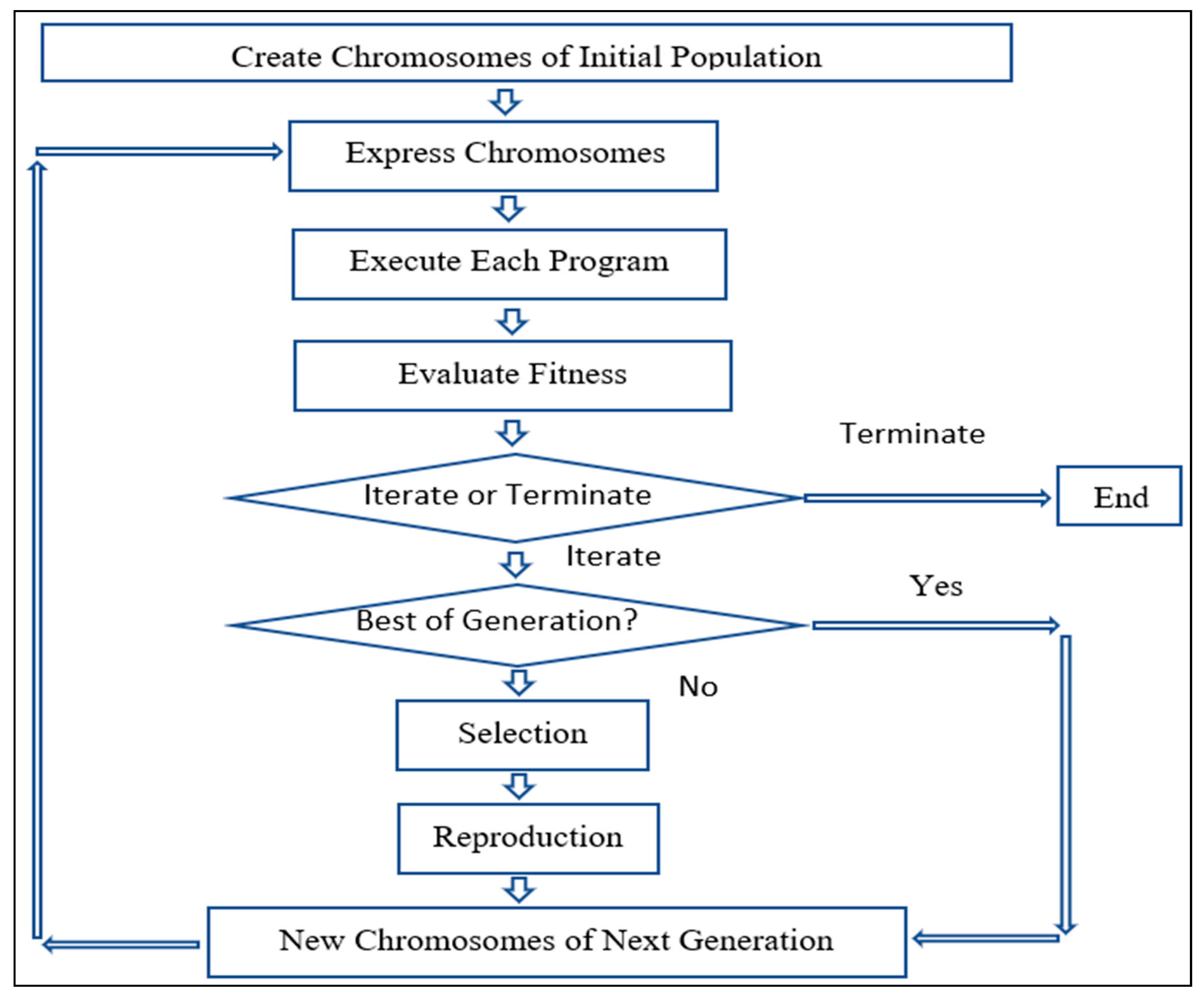
Gene expression programming (GEP) belongs to the ‘Evolutionary Algorithms’ group and, similar to other evolutionary algorithms, uses populations of individual solutions, selects and reproduces (breeds) some of them in accordance with fitness, and introduces genetic variation using mutation or recombination as prerequisites for evolution to occur [33]. A Genetic Algorithm (GA) and Genetic Programming (GP), on the other hand, are simple replicator systems with GP being more complex than GA. The fundamental difference among GA, GP, and GEP is in the nature of their individuals. The individuals are linear strings of fixed length (chromosomes) in the case of GA whereas GP consists of individuals that are of different sizes and shapes. The advantages of GP and GA are retained in GEP, making it capable of solving the coding explosion problem observed in GP while keeping the genetic operations simple similar to GA [34]. Attributes from both GA and GP are carried to GEP, and the individuals of GEP are encoded as linear strings of fixed length. These individuals are expressed in GEP as nonlinear entities afterwards having different sizes and shapes [35]. The function of Expression Trees (ETs) is to hold the genetic information. GEP follows simplistic genetic code of one-on-one relationship between symbols of the genes and the nodes of the ETs. ETs can be further divided into sub-ETs. Figure 2 shows the working principle of GEP in a brief flowchart. The model randomly generates chromosomes of initial population, expresses each individual chromosome, evaluates them based on a fitness function, and modifies the best fitted ones [36]. Evolved individuals of the new generation possess developed expressions of the genomes and evolving processes are repeated until a predefined best-fitting value is achieved or for a predefined number of generations [37].
2.3. Models Setup
2.3.1. The SWAT Model
Physiographic Data
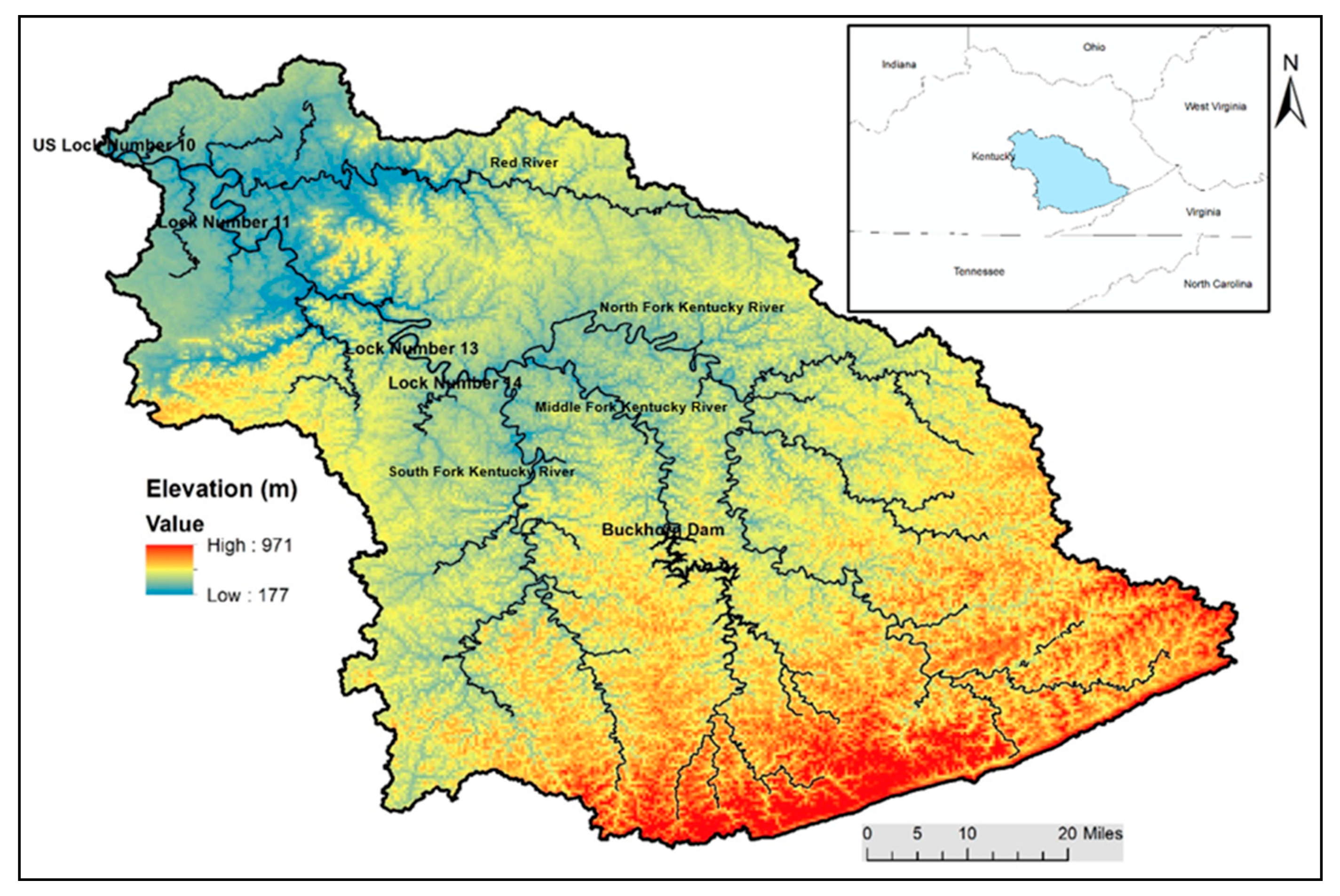
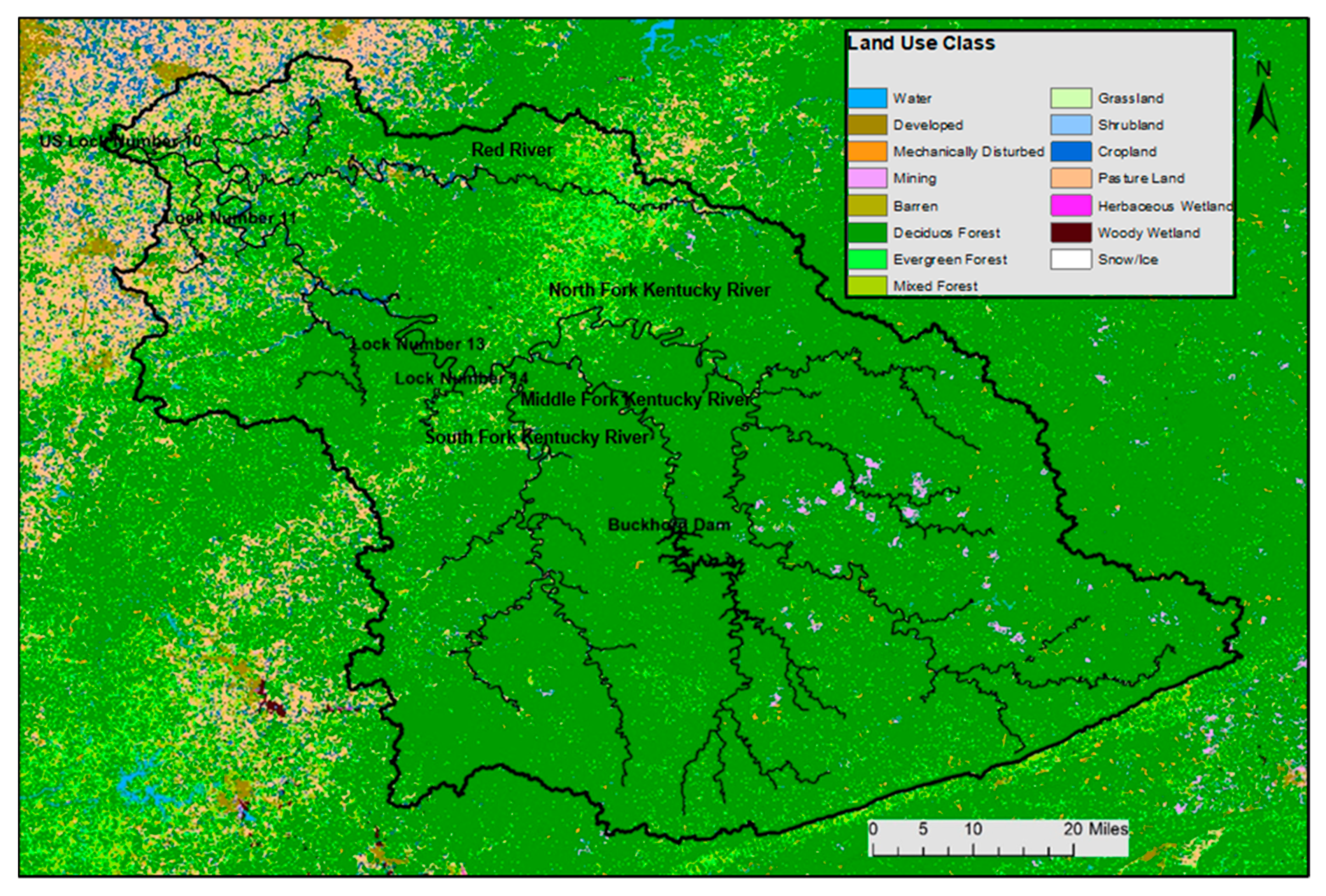
The USGS digital elevation model (DEM) data for the upper Kentucky River Basin were obtained from http://seamless.usgs.gov (accessed on 11 September 2021) (30 m × 30 m spatial resolution). The basin and watersheds were automatically delineated in the ArcGIS extension and graphical user input interface for SWAT (ArcSWAT). The elevation of the upper Kentucky River Basin ranges from 177 m to 971 m with an average elevation of 374 m above mean sea level (Figure 3). Land use data of the upper Kentucky River Basin were extracted from USGS GIRAS (Geographic Information Retrieval and Analysis System) LULC (Land Use Land Cover) files. Data gaps and overlaps were removed through manual adjustment and the final land use map was re-classified by land use groups. Deciduous forest (FRSD) is predominant in the basin (covering 84.1% of total area) while pasture (PAST) and barren (BARR) cover 11.2% and 1.9% of the area, respectively (Figure 4).
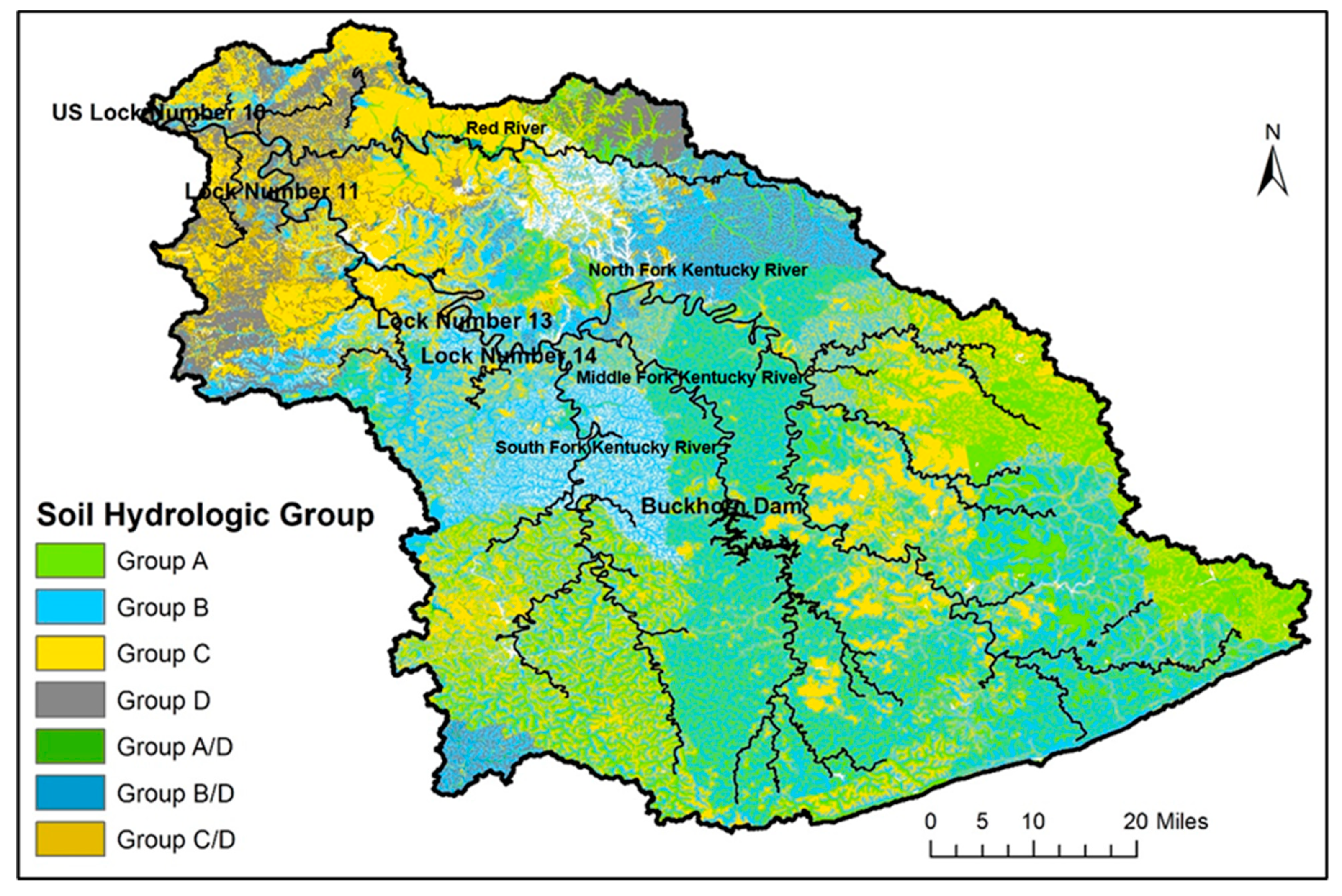
SSURGO (Soil Survey Geographic Database) soil data of the NRCS (Natural Resources Conservation Service) for the upper Kentucky River Basin were obtained from the Soil Data Mart (http://soildatamart.nrcs.usda.gov (accessed on 23 June 2021)). SSURGO soil maps allow users to link with SSURGO soil database in ArcSWAT through the MUKEY attribute. The dominant soil group in the upper Kentucky River Basin is ultisols, also known as red clay soil, covering 90% of the basin’s total area. Inceptisols and alfisols are found in scattered areas across the basin with a total area of less the 10% of the basin’s area. Figure 5 suggests that the dominant soil hydraulic group in the upper Kentucky River Basin is Group B (45%; silt loam/loam, moderately well to well drained, moderate infiltration, and runoff rate) followed by Group C (25%; sandy clay loam, low infiltration rate) and Group A (23%; sand/loamy sand/sandy loam, well drained, low runoff, high infiltration rate).
Meteorological Data
SWAT simulation requires meteorological data inputs including daily precipitation, maximum and minimum air temperature, solar radiation, humidity, and wind speed. Global Historical Climatology Network-Daily (GHCN-Daily) product from the National Climatic Data Center (NCDC) was used as the rainfall product. The product is based on observations by rain gauges within or near the basin at a daily time scale. Data were obtained from the Hydrologic Information System of the Consortium of Universities for the Advancement of Hydrologic Sciences (CUAHSI-HIS, cuahsi.org (accessed on 23 June 2021)). The CUAHSI HydroDesktop application allows users to query a specific type of data for a time-period for a specific area. Queried precipitation data for the two periods, 2002–2005 and 2008–2010, were downloaded at daily time step for 21 rain gauges. Temperature, humidity, and wind speed data were obtained from the National Climatic Data Center (NCDC) of the National Oceanic and Atmospheric Administration (NOAA) (http://gis.ncdc.noaa.gov/map/cdo/ (accessed on 23 June 2021)). These data were recorded at an hourly time-step for the study period and were averaged to daily values. Solar radiation data used in this study are satellite-based products that are estimated from NOAA Geostationary Operational Environmental Satellites (GOES) visible satellite images and were available to download at https://solaranywhere.com/ (accessed on 23 June 2021).
2.3.2. The ARX Model
The ARX model only requires daily discharge and precipitation data as input with precipitation as the exogenous variable. The ARX model uses the same precipitation time series data that have been used in the SWAT model. The selection of number of lagged days of precipitation and discharge used in the model affects the result and the optimum combination varies with the size, shape, and characteristics of the watershed [38]. The ARX models were explored with different combination of lagged days and the model with the best performance is the one with three lagged days of precipitation and discharge. The following equation was used to calculate the simulated discharge:
where Q(t) is the simulated discharge; Q(t − 1), Q(t − 2), and Q(t − 3) are lagged discharges; P(t − 1), P(t − 2), and P(t − 3) are lagged precipitations; 1–6 are coefficients obtained through regression; and C is the intercept.
2.3.3. The GEP Model
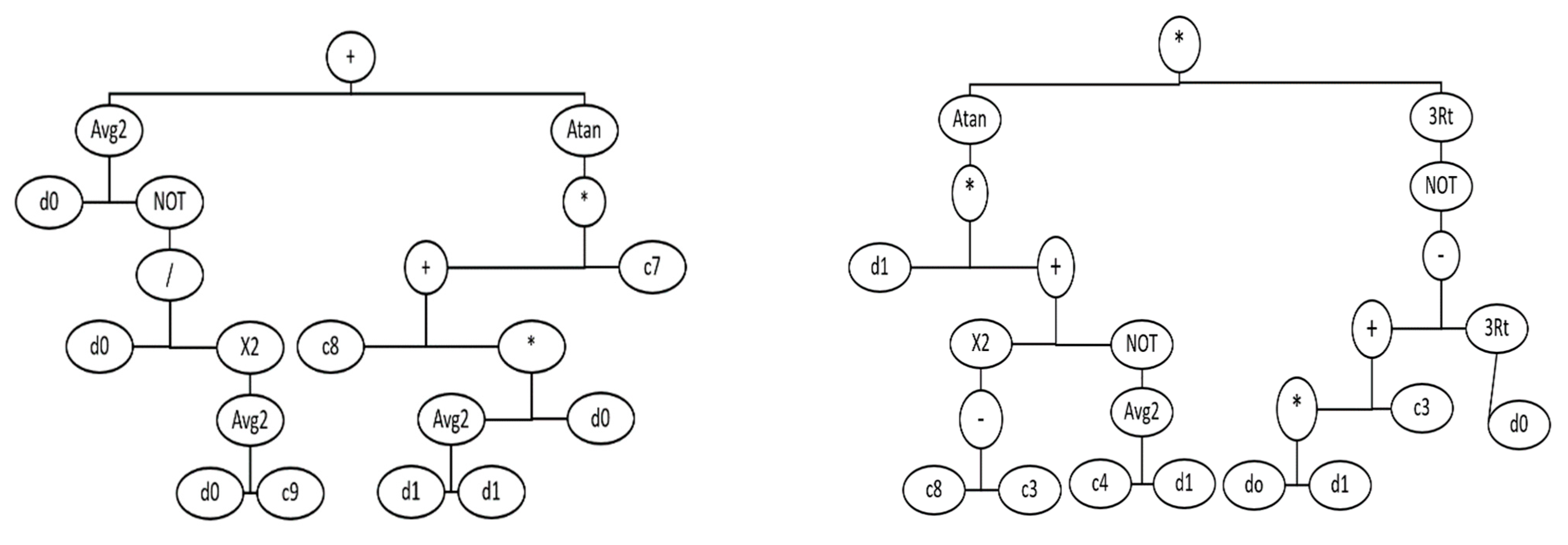
One of the main advantages of data-driven models is the simplicity of data and elimination of complexities of physically-based models [39]. The solution model is typically an easy-to-track linear or non-linear formula that relates the dependent and independent variables, and the user can control the complexity of the solution model. This study used the commercial software GeneXproTools 5.0 for GEP modelling in which appropriate dataset(s) are fed as input and the software can analyze the input dataset(s) and gives the best model(s) to fit the observed output. Discharge data alone or discharge data along with precipitation data can be used as input data for the models with the output being the one-day-ahead discharge. Selection of mathematical functions (e.g., Sqrt, Exp, Ln, Log, x^t, Sine, Cosine, average, among many more) for the model can either be performed manually or the software can select the most appropriate functions. The best performing model is selected from numerous generated models and the expression tree (ET) of the selected model includes nine sub-ETs. The sub-ET 7 and the sub-ET 9 of the selected model (Figure 6) are expressed by the algebraic formulas in Equations (7) and (8):
where .
where .
Here, A, B, C, D, E, F, G, and H are simplified forms to express mathematical formulas with less complexity. d0 is precipitation of the day in which discharge is to be predicted and d1 is discharge of the previous day of prediction day. c0, c1, c2, c3, c4, c5, c6, c7, c8, and c9 are numerical constants for each gene. The selected model contains total nine genes and the values of c0 to c9 varies for each gene. These sub-ETs are considered as phenotypes while the genotypes are as follows:
Genotype for sub-ET 9:
∗ Atan 3Rt ∗ NOT d1 + − X2 NOT + 3Rt – Avg2 ∗ c3 d0 c8 c3 c4 d1 d0 d1
Genotype for sub-ET 7:
+ Avg2 Atan d0 NOT ∗/+ c7 d0 X2 c8 ∗ Avg2 Avg2 d0 d0 c9 d1 d1
2.4. Observed Discharge Data
Daily discharge data recorded at two stream gauges, USGS 03282000 at Heidelberg, Kentucky and USGS 03284000 near Winchester, Kentucky were used in this study. USGS 03282000 stream gauge measures discharge at the confluence of North Fork Kentucky River, Middle Fork Kentucky River, and the South Fork Kentucky River and represents the natural flow of the upper Kentucky River as it is located upstream of all the locks and dams. Meanwhile, USGS 03284000 stream gauge measures the outlet of the whole upper Kentucky River. Located downstream of four locks and dams (LD 11, 12, 13, and 14) on the main stem of upper Kentucky River, discharge at USGS 03284000 stream gauge is affected by the operation of the four LDs.
In general, discharge recorded at the downstream station, USGS 03284000, is higher than that measured at USGS 03282000 station because the river gains more water from downstream tributaries. Figure 7 shows time series of daily flows recorded at the two stations during the calibration and validation periods. On average, discharge at the downstream station is 26% and 23% higher for the calibration and validation periods, respectively. However, the flow at the downstream station is sometimes lower than that at the upstream stream. For instance, the peak flows during the rainfall events in January and May 2002 or in April, June, and September 2003 present are lower discharge at USGS 03284000 at the downstream station. That is mainly due to the flow regulation by the dams between the two stations. However, on average, measured discharge at USGS 03284000 gauge is about 30% lower than value at above measuring location in those periods.
2.5. Model Performance Evaluation
Three standard statistical measures were used in the model performance evaluation: correlation coefficient (R), Nash-Sutcliffe Efficiency (NSE), and Error in runoff volume (Bias). These measures are defined as follows:
where and represents the observed and the simulated discharge (on day t), respectively; and represents the average of the observed and the simulated discharge, respectively; and N represents the total number of records.
The degree of linear correlation (between the simulated and the observed discharge time series) can be evaluated using the R2 statistical measure (value of 1 indicates the perfect match between the simulated and the observed discharge [40]. The NSE indicates the ability of the model to reproduce observed discharge and holds values smaller or equal to 1 [41]. Larger NSE values imply high ability of in reproducing the observed data. E_peak and E_runoff measure the percentage differences between simulated and observed peak flow runoff volume, respectively. Table 1 represents the performance ratings of NSE, R2, and PBIAS:
2.6. Model Calibration and Validation
For all three models, the natural flow of the upper Kentucky River for the period of 2002–2005 as observed by USGS 03282000 stream gauge above LD 14 was used for calibration. When necessary, manual calibration was performed by modifying values of model parameters individually to reach the best fit between simulated and observed discharge. For the SWAT model, the calibration involved adjusting the values of several parameters. SWAT outputs were more sensitive to CH_N2 (Manning’s N value for stream channels), CN2 (Soil Conservation Service (SCS) curve numbers), SOL_K (soil hydraulic conductivity), and SOL_AWC (available water capacity of the soil). Other parameters with less impact on model outputs, such as ALPHA_BF (base flow alpha factor), ESCO (soil evaporation compensation factor), and GW_REVAP (groundwater “revap” coefficient) were also included in the calibration. In case of the ARX model, several combinations were tried out with different numbers of lagged days of precipitation and discharge to obtain the combination with the best agreement between the ARX-predicted and observed one-day-ahead discharge was identified. For the GEP model, the number of chromosomes and genes, the head size, and the linking functions were controlled manually with several iterations to obtain the best model combination.
For validation, the calibrated models were used to predict daily discharge at the calibration stream gauge and for the entire upper Kentucky River Basin with the outlet near USGS 03284000 stream gauge for the 2008–2010 period. Validation at the downstream station assesses the effect of regulation on the discharge predictability and how the calibrated model can simulate the basin response beyond the calibration area.
3. Results and Discussion
3.1. Calibration Results
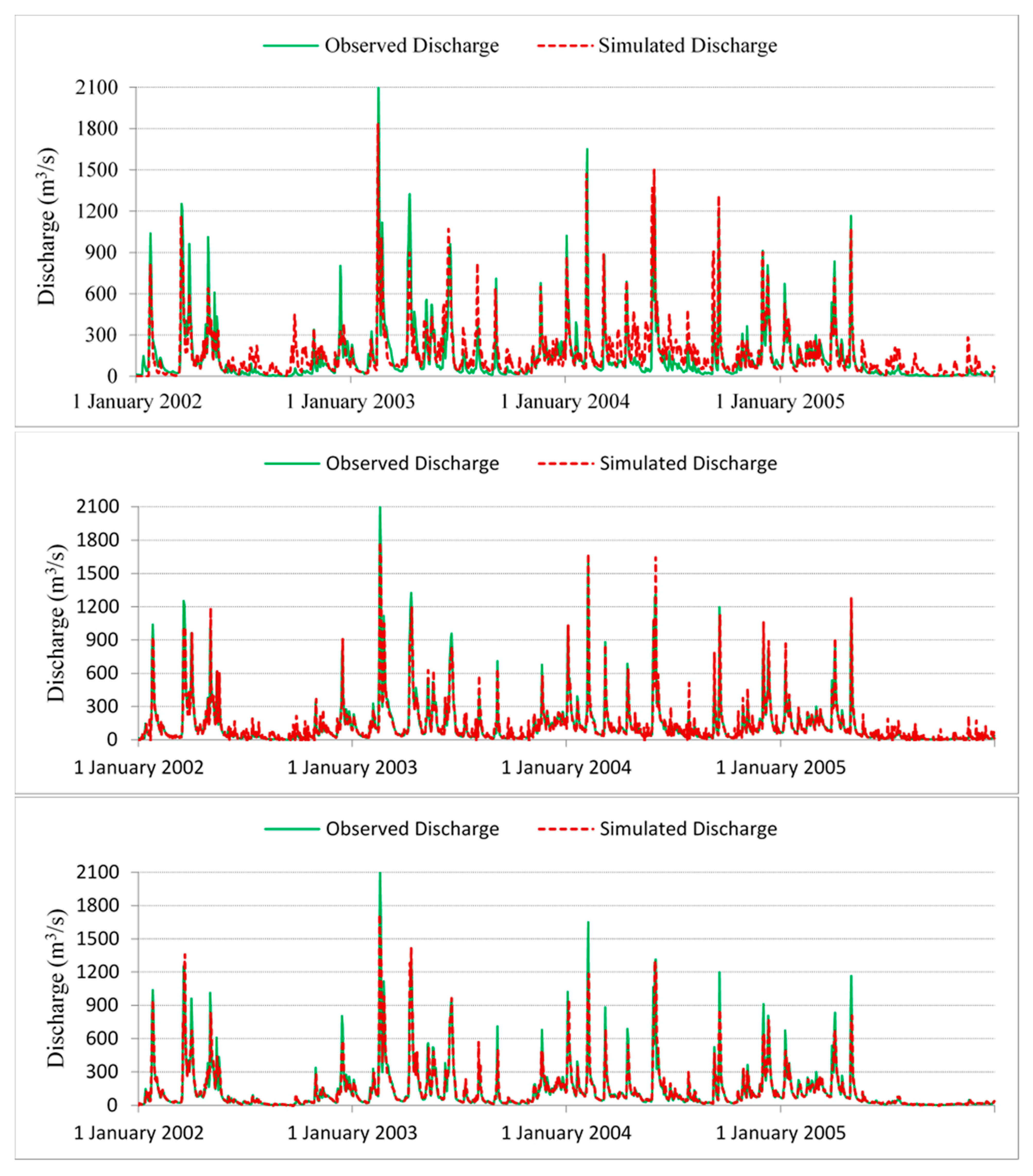
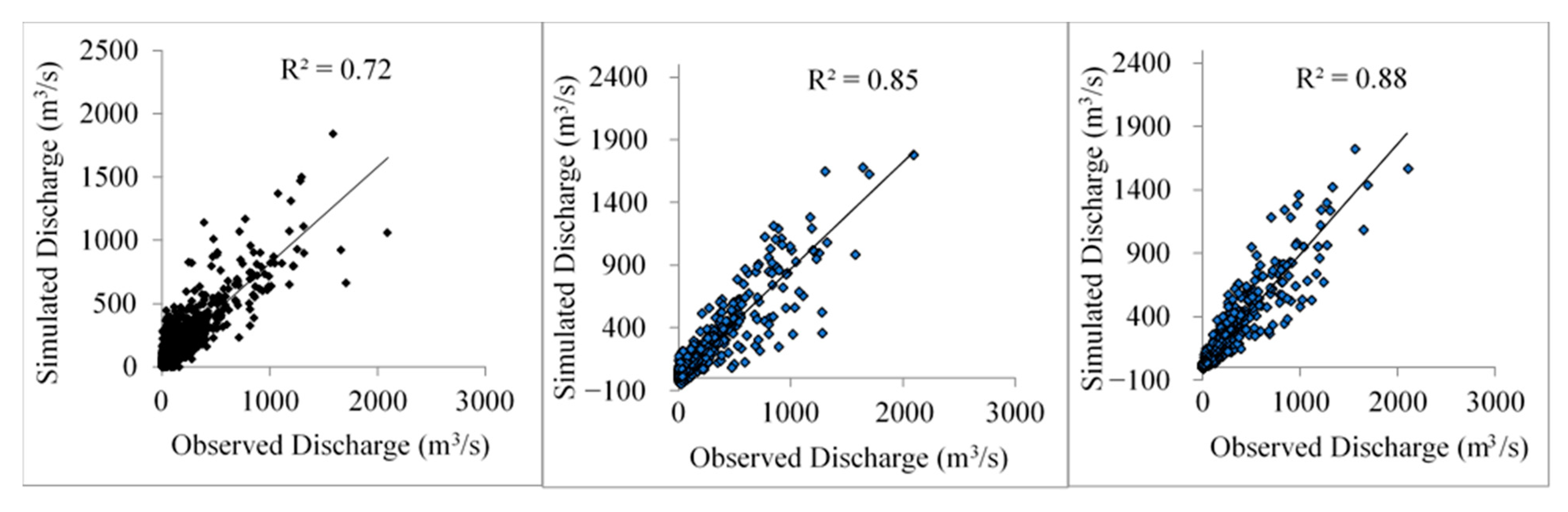
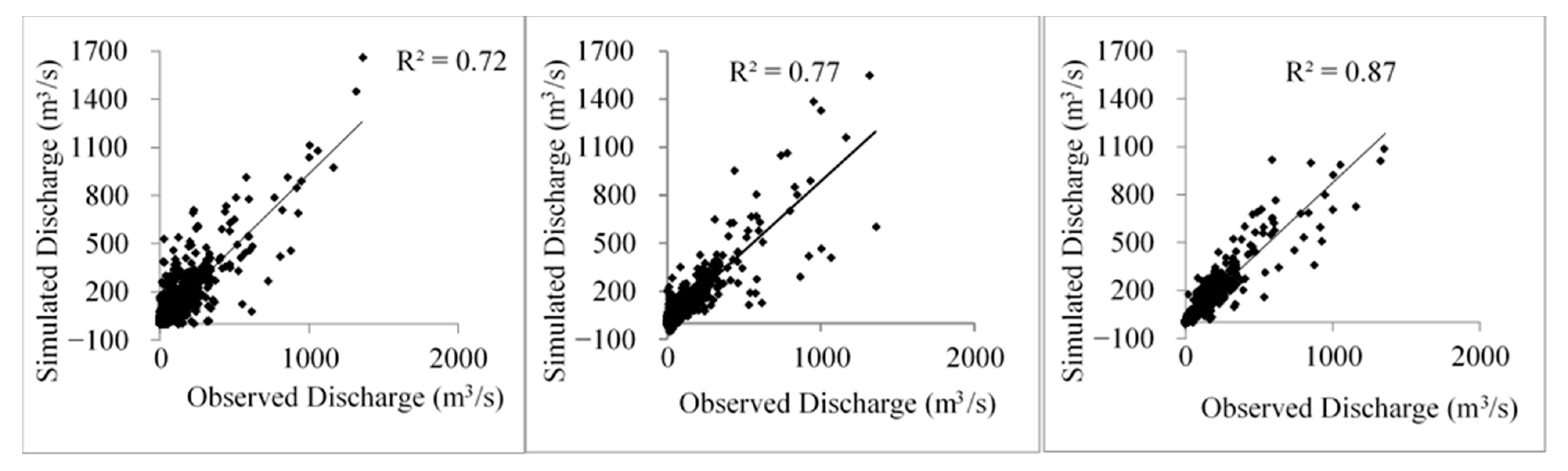
The 4-year calibration period included numerous rainfall events with an average annual precipitation of 1360 mm (16% above average). Initially, the SWAT model was run using the default values of model parameters and the result from the un-calibrated model overestimated both the base-flows and the peaks of Kentucky River discharge. The model was then calibrated manually with the objective of obtaining the best values of the statistical measures described above. Table 2 presents the calibrated values of the major SWAT model parameters. The SWAT model was able to adequately reproduce the daily discharge (Figure 8 and Figure 9) with good R2 and NSE values of 0.72 and 0.71, respectively (Table 3). The errors in peak discharge and runoff volume were 10.1% and 16.9%, respectively.
Data-driven models require no input parameters for calibration. In this study, only lagged-day discharge and precipitation data were used, and the best prediction statistical measures were obtained with three previous time steps of rainfall and one previous time step of streamflow observations as inputs for both models (ARX and GEP). For the ARX model, the R2, NSE, and bias for the calibration are 0.85, 0.85, and −0.02%, respectively (Table 3). The same measures for the GEP model are 0.88, 0.88, and −0.17%, respectively (Table 3). These measures indicate that the GEP and ARX models clearly outperform the SWAT model with the GEP model producing the best calibration results.
SWAT model performance generally improved in the last 2 years of the calibration period because such a physically based model needs a spin-up time for the effects of errors in assumed initial conditions estimates to diminish. ARX and GEP, on the other hand, are data-driven models and do not require any warm-up period. Their performances in individual years appear to be random and no specific trend was observed.
3.2. Validation Results
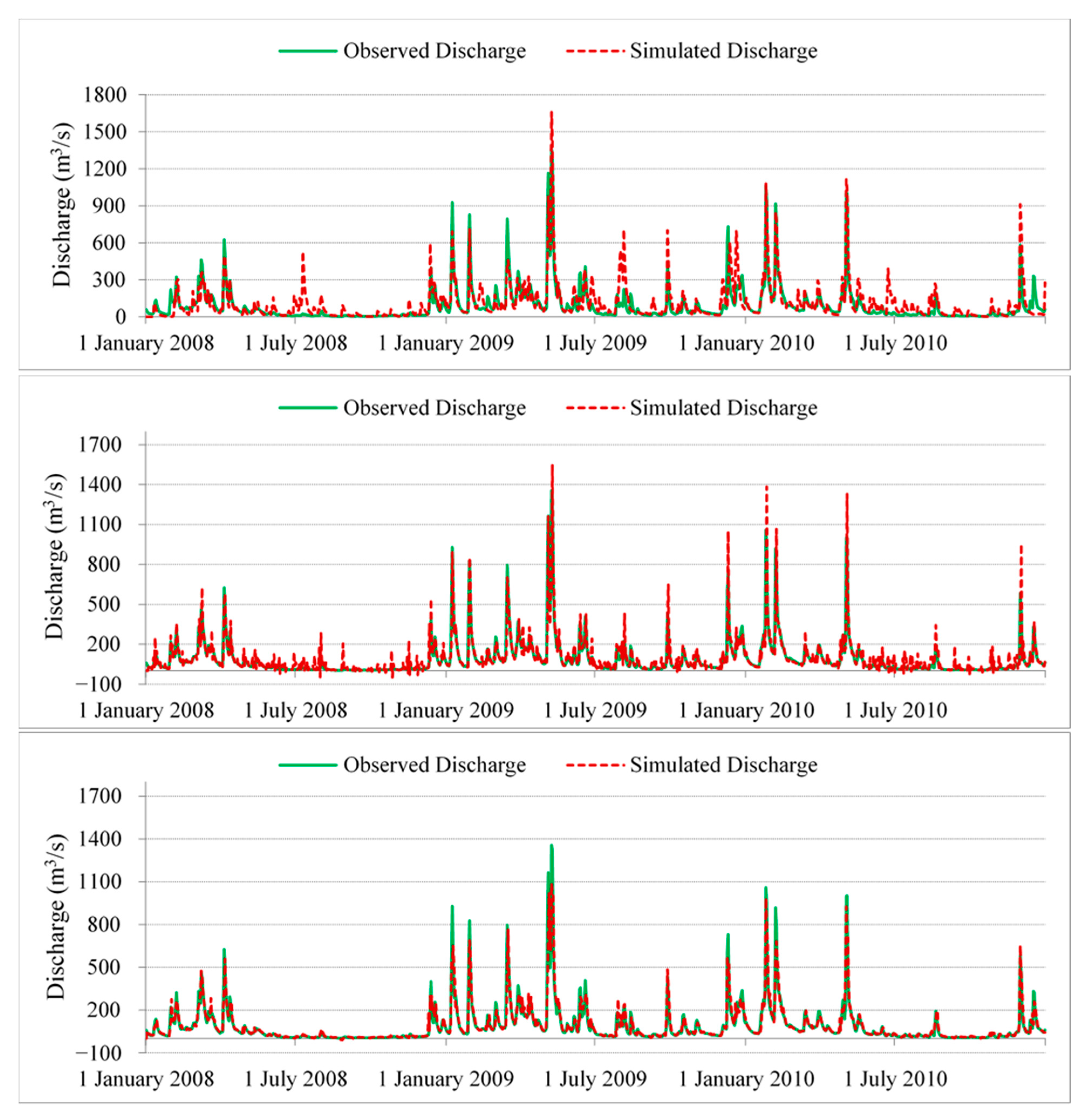
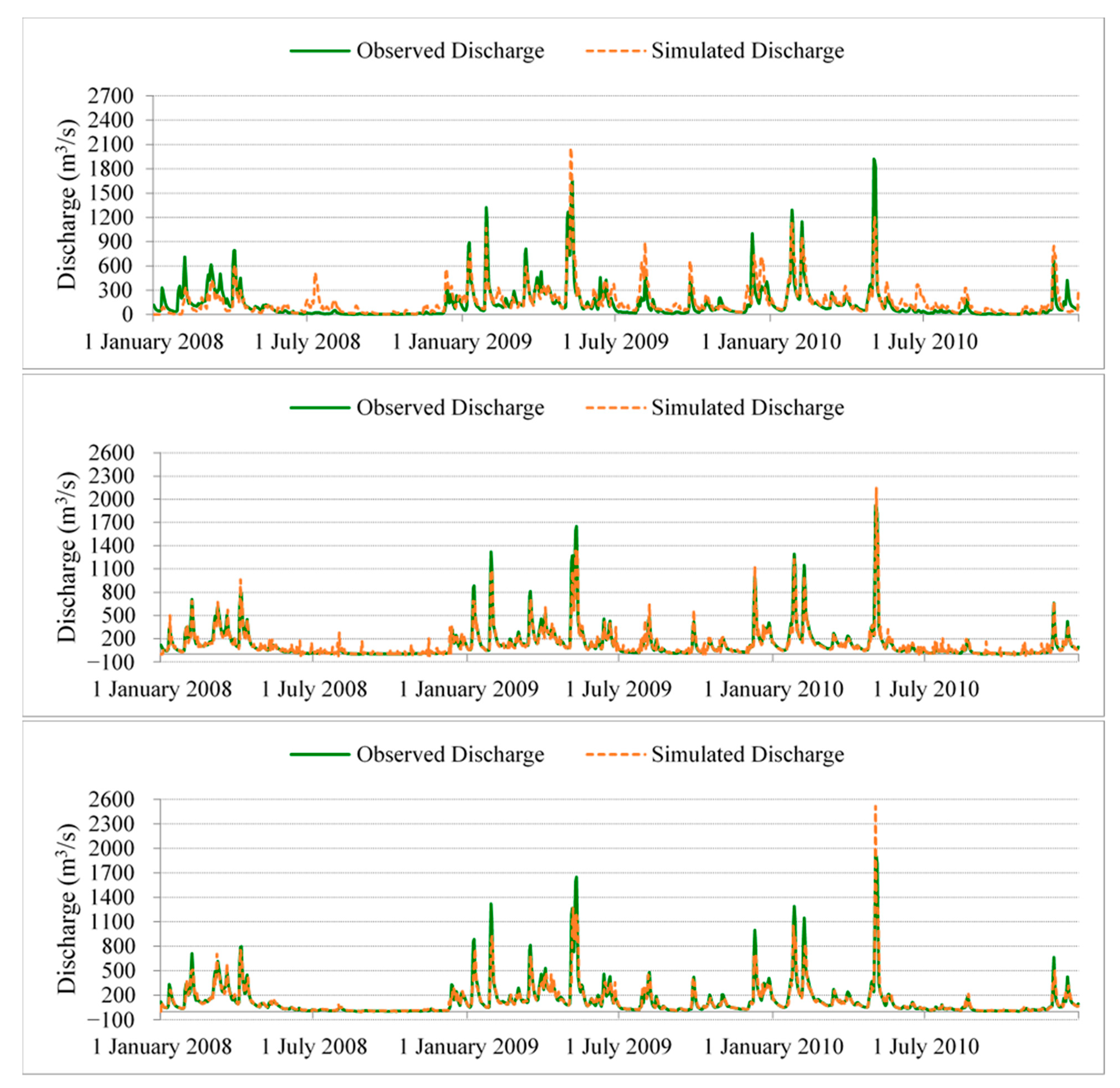
The three models were validated for the period 2008–2010, which had an average annual precipitation of about 10% lower than the calibration period. As mentioned earlier, validation was performed at LD14 where models were calibrated and at LD10, which is located approximately 88 km downstream. The comparison between observed and simulated daily discharge at LD14 and LD10 during validation period of 2008–2010 is represented in Figure 10 and Figure 11. The statistical performance measures are summarized in Table 4.
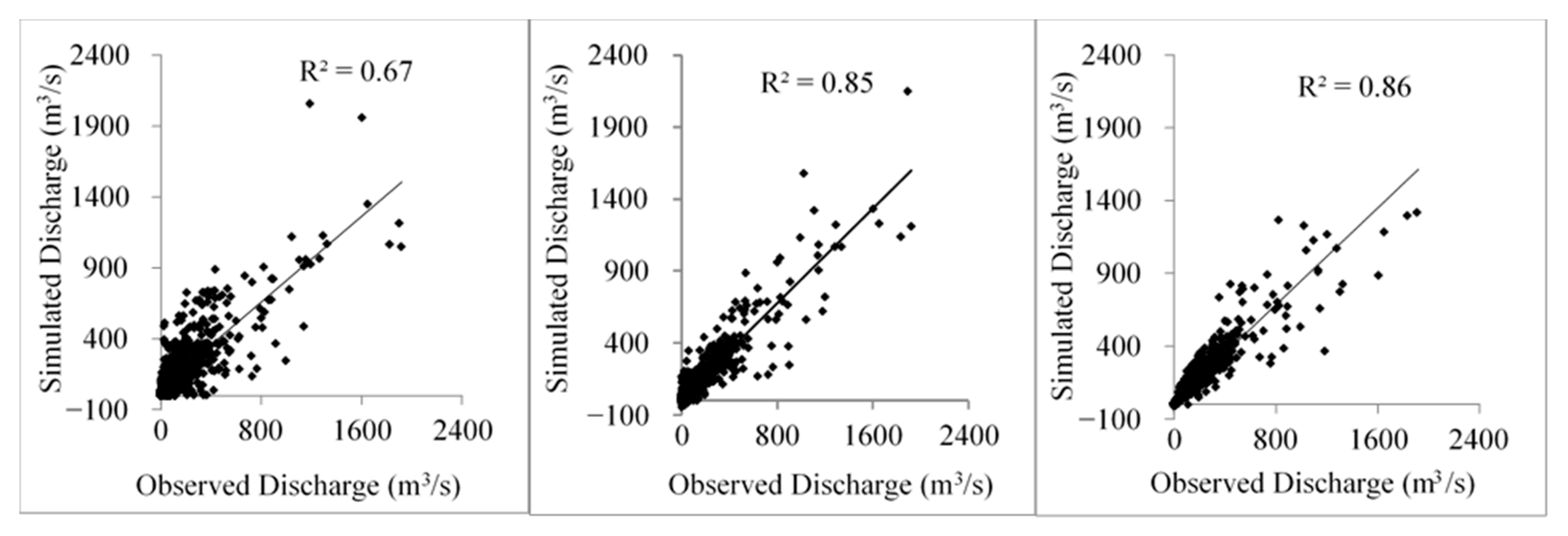
Figure 12 and Figure 13 and Table 4 indicate that GEP model has the best performance at both locations with very good performance rating which is consistent with prior studies [14,36,45]. As in the calibration results, GEP model outperformed the other two models with R2 values of 0.86 and 0.87 and NSE values of 0.86 and 0.87 for validation at LD10 and LD14, respectively. However, the ARX model and the GEP model provided similar performance at LD10. The performance of the ARX model is similar to the previous studies (good/very good performance rating) in one-day-ahead discharge prediction [46,47]. The SWAT model displayed moderate performance with NSE of about 0.65 and an R2 value of about 0.64. This observation is in agreement with the previous studies which concluded performance rating of SWAT model was satisfactory or good [48,49,50]. It is very clear that both GEP and ARX perform better than SWAT during low-flow periods.
Statistical analysis of SWAT results indicates that the model performed better during the second and the third year of validation period. This once more suggests that the model performance significantly improved after a warm-up period. ARX and GEP do not have this problem. Moreover, ARX and GEP are much less affected by the length of the calibration period compared to SWAT. For example, using only 1 year in calibrating the models reduced by SWAT validation NSE values by more than 25% while NSE in the ARX model deteriorated by about 5% and GEP performance remained virtually unaffected. It is well known in hydrology that the spatio-temporal and spatial heterogeneity of precipitation and watershed characteristics and the myriad of processes involved in runoff and discharge generation make the rainfall–runoff relationships highly nonlinear, complex, and hard to accurately simulate. The SWAT model was run at daily time step in this study due to the resolution of precipitation data, which could have affected its performance. Moreover, the output of SWAT depends on the accuracy of the input data, which can never be guaranteed. Additionally, more vigorous calibration of SWAT model could have improved the accuracy of its predictions. Nonetheless, the SWAT results reported in this study are not inferior to those reported in similar studies.
4. Conclusions
Streamflow forecasting is of enormous importance for water budget planning and numerous operational water resources application. The study demonstrates that machine learning (ML) techniques can be useful in the prediction of hydrologic variables, such as streamflow, particularly when the underlying processes have complex nonlinear interrelationships. However, many ML techniques, unlike GEP, do not produce solutions that provide insight into the explicit relationship between input and output variable. These characteristics are illustrated using a simple, though very widely used, autoregressive model and a classic hydrologic prediction problem. The Kentucky River case study demonstrates the superiority of GEP and its ability to provide fast, relatively accurate, and computationally inexpensive estimation of the underlying physical/functional processes that are employable beyond forecast applications. This study used SWAT, ARX, and GEP models to simulate daily river discharge of the Upper Kentucky River to examine the capability of the three models to reproduce river discharge using four evaluation metrics.
The two data-driven models outperformed the physically based SWAT model, which produced less accurate but still acceptable results. The performance metrics indicate that the GEP model provided the best performance with the ARX model being not far off. The SWAT model overestimated runoff and underestimated peak discharge while the ARX and GEP models underestimated the peak discharge. Runoff is mostly underestimated by GEP and ARX except for a few exceptions. The percentage of error in predicting peak discharge and runoff was higher for the hydrologic model than data-driven models most of the time. Research results also suggest that a warm-up period (1 or 2 years) is necessary for SWAT to achieve improved and reliable performance. Performance of data-driven models, however, exhibits no specific trend with time and largely dependent on selection of modelling datasets and adaptation of methods. Overall, statistical measures for model calibration and validation suggest that the data-driven models, specially the GEP model, provided outstanding performance to reproduce daily discharge in alternative locations of the Upper Kentucky River under changing climatic variables.
A major advantage of GEP, unlike many other data-based models, is that it can provide an analytical form of the relationship between input and output variables. This will allow modelers to gain insight into this relationship and perform modifications if necessary. This study used the GEP model in its simplest form. Modelers also have the flexibility to improve the prediction capability of the GEP model by judiciously including additional input variables that can affect the basin response, e.g., temperature. GEP models can be further improved by preprocessing the input data, e.g., by applying wavelet-de-noising or modeling low- and high-flow periods separately [51]. The flexibility of GEP suggests immense potential applications in hydrometeorology such as estimation of precipitation, evapotranspiration, and soil moisture based on direct and indirect measurements. In general, GEP will allow progressive model identification when new data become available by adapting the functional relationship for the former and modifying the parameters of the latter in addition to the recursive model updating that allows to track temporal changes. Lastly, unlike the SWAT model, GEP and ARX model do not require a spin-up period as they are less sensitive to the extent of the calibration time series.
Author Contributions
H.O.S. guided this research, contributed significantly to preparing the manuscript for publication, and contributed to developing the research methodology; K.B. and T.B.L. processed the data, developed the scripts used in the analysis, and performed the analysis; K.B. and T.B.L. prepared the first draft; H.O.S. performed the final overall proof reading of the manuscript. All authors read and agreed to the published version of the manuscript.
Funding
This research received no external funding.
Institutional Review Board Statement
Not applicable.
Informed Consent Statement
Not applicable.
Data Availability Statement
Publicly available datasets were analyzed in this study. The data can be found at http://gis.ncdc.noaa.gov/map/cdo/ and https://solaranywhere.com/ (accessed on 23 June 2021).
Conflicts of Interest
The authors declare no conflict of interest.
References
- Price, K. Effects of watershed topography, soils, land use, and climate on baseflow hydrology in humid regions: A review. Prog. Phys. Geogr. Earth Environ. 2011, 35, 465–492. [Google Scholar] [CrossRef]
- Van Liew, M.W.; Arnold, J.G.; Garbrecht, J.D. Hydrologic simulation on agricultural watersheds: Choosing between two models. Trans. ASAE 2003, 46, 1539–1551. [Google Scholar] [CrossRef]
- Clark, M.P.; Bierkens, M.F.P.; Samaniego, L.; Woods, R.A.; Uijlenhoet, R.; Bennett, K.E.; Pauwels, V.R.N.; Cai, X.; Wood, A.W.; Peters-Lidard, C.D. The evolution of process-based hydrologic models: Historical challenges and the collective quest for physical realism. Hydrol. Earth Syst. Sci. 2017, 21, 3427–3440. [Google Scholar] [CrossRef] [Green Version]
- Barnhart, B.L.; Golden, H.E.; Kasprzyk, J.R.; Pauer, J.J.; Jones, C.E.; Sawicz, K.A.; Hoghooghi, N.; Simon, M.; McKane, R.B.; Mayer, P.M.; et al. Embedding co-production and addressing uncertainty in watershed modeling decision-support tools: Successes and challenges. Environ. Model. Softw. 2018, 109, 368–379. [Google Scholar] [CrossRef]
- Knisel, W.G. CREAMS: A Field Scale Model for Chemicals, Runoff, and Erosion from Agricultural Management Systems; Conservation Research Report; U.S. Department of Agriculture: Washington, DC, USA, 1980. [Google Scholar]
- Leavesley, G.H.; Lichty, R.W.; Troutman, B.M.; Saindon, L.G. Precipitation-runoff modeling system: User’s manual. Water-Resour. Investig. Rep. 1983, 83, 207. [Google Scholar]
- Johanson, R.C.; Imhoff, J.C.; Little, J.L.; Donigian, A.S. User’s Manual for the Hydrological Simulation Program (HSPF); U.S. Environmental Protection Agency: Athens, GA, USA, 1984. [Google Scholar]
- Arnold, J.G.; Allen, P.M.; Bernhardt, G. A Comprehensive Surface-Groundwater Flow Model. J. Hydrol. 1993, 142, 47–69. [Google Scholar] [CrossRef]
- Luijten, J. Dynamic Hydrological Modeling Using ArcView GIS. ArcUser, July–September; ESRI: Redlands, CA, USA, 2000. [Google Scholar]
- Bingner, R.L. Runoff Simulated from Goodwin Creek Watershed Using SWAT. Trans. ASAE 1996, 39, 85–90. [Google Scholar] [CrossRef]
- Rauf, A.; Ghumman, A.R. Impact Assessment of Rainfall-Runoff Simulations on the Flow Duration Curve of the Upper Indus River—A Comparison of Data-Driven and Hydrologic Models. Water 2018, 10, 876. [Google Scholar] [CrossRef] [Green Version]
- Parasuraman, K.; Amin, E.; Sean, K.C. Modelling the dynamics of the evapotranspiration process using genetic programming. Hydrol. Sci. J. 2007, 52, 563–578. [Google Scholar] [CrossRef]
- Barge, J.T.; Sharif, H.O. An Ensemble Empirical Mode Decomposition, Self-Organizing Map, and Linear Genetic Programming Approach for Forecasting River Streamflow. Water 2016, 8, 247. [Google Scholar] [CrossRef] [Green Version]
- Aytek, A.; Asce, M.; Alp, M. An application of artificial intelligence for rainfall-runoff modeling. J. Earth Syst. Sci. 2008, 117, 145–155. [Google Scholar] [CrossRef] [Green Version]
- U.S. EPA (U.S. Environmental Protection Agency). Mountaintop Mining/Valley Fills in Appalachia—Final Programmatic Environmental Impact Statement. 2005. Available online: http://www.epa.gov/region03/mtntop/index.htm (accessed on 27 November 2020).
- Kentucky River and Tributaries. Upper Kentucky River Navigation Project. Volume 2. Public Involvement Record. Army Engineer District Louisville KY. 1980. Available online: https://apps.dtic.mil/sti/citations/ADA115625 (accessed on 27 November 2020).
- KGS (Kentucky Geological Survey). Kentucky River Basin Map and Chart by Carey, D.I. 2009. Available online: http://kgs.uky.edu/kgsweb/olops/pub/kgs/mc188_12.pdf (accessed on 17 June 2021).
- USGS (U.S. Geological Survey). Water-Quality Assessment of the Kentucky River Basin, Kentucky—Analysis of Available Surface-Water-Quality Data Through 1986; National Water-Quality Assessment: Reston, VA, USA, 1995; USGS Water-Supply Paper 2351.
- Kentucky River Authority. Kentucky River History—Locks and Dams. 2021. Available online: http://finance.ky.gov/offices/Pages/LocksandDams.aspx (accessed on 17 June 2021).
- Kentucky River Locks and Dams. Available online: https://abandonedonline.net/location/kentucky-river-locks-dams/ (accessed on 11 September 2021).
- Kentucky River Authority. Available online: https://finance.ky.gov/kentucky-river-authority/PublishingImages/kyriverbasinmap.jpg (accessed on 23 August 2021).
- Arnold, J.G.; Srinivasan, R.; Muttiah, R.S.; Williams, J.R. Large area hydrologic modeling and assessment—Part I: Model development. J. Am. Water Resour. Assoc. 1998, 34, 73–89. [Google Scholar] [CrossRef]
- Arnold, J.G.; Kiniry, J.R.; Srinivasan, R.; Williams, J.R.; Haney, E.B.; Neitsch, S.L. Soil and Water Assessment Tool Input/Output File Documentation Version 2009; Technical Report No. 365; Texas Water Resources Institute: College Station, TX, USA, 2010. [Google Scholar]
- Chaplot, V.; Saleh, A.; Jaynes, D.B.; Arnold, J. Predicting water, sediment and NO3-N loads under scenarios of land-use and management practices in a flat watershed. Water Air Soil Pollut. 2004, 154, 271–293. [Google Scholar] [CrossRef]
- Abbaspour, K.C.; Yang, J.; Maximov, I.; Siber, R.; Bogner, K.; Mieleitner, J.; Zobrist, J.; Srinivasan, R. Modelling hydrology and water quality in the pre-alpine/alpine Thur watershed using SWAT. J. Hydrol. 2007, 333, 413–430. [Google Scholar] [CrossRef]
- Rostamian, R.; Jaleh, A.; Afyuni, M.; Mousavi, S.F.; Heidarpour, M.; Jalalian, A.; Abbaspour, K.C. Application of a SWAT model for estimating runoff and sediment in two mountainous basins in central Iran. Hydrol. Sci. J. 2008, 53, 977–988. [Google Scholar] [CrossRef]
- Yahya, C. Using ARX and NARX approaches for modeling and prediction of the process behavior: Application to a reactor-exchanger. Asia-Pac. J. Chem. Eng. 2008, 3, 597–605. [Google Scholar] [CrossRef]
- Knotters, M.; Bierkens, M.F.P. Physical basis of time series models for water table depths. Water Resour. Res. 2000, 36, 181–188. [Google Scholar] [CrossRef]
- James, L.D.; Thompson, W.O. Least Squares Estimation of Constants in a Linear Recession Model. Water Resour. Res. 1970, 6, 1062–1069. [Google Scholar] [CrossRef]
- Tallaksen, L.M. A review of baseflow recession analysis. J. Hydrol. 1995, 165, 349–370. [Google Scholar] [CrossRef]
- Ljung, L. System Identification. In Signal Analysis and Prediction; Applied and Numerical Harmonic Analysis; Prochazka, A., Kingsbury, N.G., Payner, P.J.W., Uhlir, J., Eds.; Springer Birkhäuser: Boston, MA, USA, 1998; pp. 163–173. ISBN 978-1-4612-7273-1. [Google Scholar]
- Wallin, R.; Isaksson, A.J.; Ljung, L. An iterative method for identification of ARX models from incomplete data. In Proceedings of the 39th IEEE Conference on Decision and Control (Cat. No.00CH37187), Sydney, NSW, Australia, 12–15 December 2000; Volume 1, pp. 203–208. [Google Scholar]
- Ferreira, C. Gene Expression Programming and the Evolution of Computer Programs. In Recent Developments in Biologically Inspired Computing; IGI Global: Hershey, PA, USA, 2005. [Google Scholar] [CrossRef]
- Gan, Z.; Yang, Z.; Li, G.; Jiang, M. Automatic Modeling of Complex Functions with Clonal Selection-Based Gene Expression Programming. Third Int. Conf. Nat. Comput. 2007, 4, 228–232. [Google Scholar] [CrossRef]
- Ferreira, C. Gene Expression Programming: A New Adaptive Algorithm for Solving Problems. Complex Syst. 2001, 13, 87–129. [Google Scholar]
- Aytac, G.; Ali, A. New Approach for Stage–Discharge Relationship: Gene-Expression Programming. J. Hydrol. Eng. 2009, 14, 812–820. [Google Scholar] [CrossRef]
- Ferreira, C. Gene Expression Programming in Problem Solving. In Soft Computing and Industry; Springer: London, UK, 2002; pp. 635–653. ISBN 978-1-4471-1101-6. [Google Scholar]
- González-Leiva, F.; Valdés-Pineda, R.; Valdés, J.B.; Ibáñez-Castillo, L.A. Assessing the Performance of Two Hydrologic Models for Forecasting Daily Streamflows in the Cazones River Basin (Mexico). Open J. Mod. Hydrol. 2016, 6, 168. [Google Scholar] [CrossRef] [Green Version]
- Brown, J.D.; Heuvelink, G.B.M. Assessing Uncertainty Propagation through Physically Based Models of Soil Water Flow and Solute Transport. In Encyclopedia of Hydrological Sciences; John Wiley & Sons: Hoboken, NJ, USA, 2006. [Google Scholar] [CrossRef] [Green Version]
- Healy, M.J.R. The Use of R2 as a Measure of Goodness of Fit. J. R. Stat. Soc. Ser. A 1984, 147, 608–609. [Google Scholar] [CrossRef]
- Nash, J.E.; Sutcliffe, J.V. River flow forecasting through conceptual models part I—A discussion of principles. J. Hydrol. 1970, 10, 282–290. [Google Scholar] [CrossRef]
- Moriasi, D.N.; Arnold, J.G.; Van Liew, M.W.; Bingner, R.L.; Harmel, R.D.; Veith, T.L. Model evaluation guidelines for systematic quantification of accuracy in watershed simulations. ASABE 2007, 50, 885–900. [Google Scholar] [CrossRef]
- Legates, D.R.; McCabe, G.J. Evaluating the use of “goodness-of-fit” measures in hydrologic and hydroclimatic model validation. Water Resour. Res. 1999, 35, 233–241. [Google Scholar] [CrossRef]
- Sakib, S.; Ghebreyesus, D.; Sharif, H.O. Performance Evaluation of IMERG GPM Products during Tropical Storm Imelda. Atmosphere 2021, 12, 687. [Google Scholar] [CrossRef]
- Khatibi, R.; Ghorbani, M.A.; Kashani, M.H.; Kisi, O. Comparison of three artificial intelligence techniques for discharge routing. J. Hydrol. 2011, 403, 201–212. [Google Scholar] [CrossRef]
- Bogner, K.; Pappenberger, F. Multiscale error analysis, correction, and predictive uncertainty estimation in a flood forecasting system. Water Resour. Res. 2011, 47. [Google Scholar] [CrossRef] [Green Version]
- Firat, M. Comparison of Artificial Intelligence Techniques for river flow forecasting. Hydrol. Earth Syst. Sci. 2008, 12, 123–139. [Google Scholar] [CrossRef] [Green Version]
- Vilaysane, B.; Takara, K.; Luo, P.; Akkharath, I.; Duan, W. Hydrological Stream Flow Modelling for Calibration and Uncertainty Analysis Using SWAT Model in the Xedone River Basin, Lao PDR. Procedia Environ. Sci. 2015, 28, 380–390. [Google Scholar] [CrossRef] [Green Version]
- Lubini, A.; Adamowski, J. Assessing the Potential Impacts of Four Climate Change Scenarios on the Discharge of the Simiyu River, Tanzania Using the SWAT Model. 2013. Available online: http://www.taccire.sua.ac.tz/handle/123456789/286 (accessed on 13 September 2021).
- Xie, H.; Lian, Y. Uncertainty-based evaluation and comparison of SWAT and HSPF applications to the Illinois River Basin. J. Hydrol. 2013, 481, 119–131. [Google Scholar] [CrossRef]
- Abdollahi, S.; Raeisi, J.; Khalilianpour, M.; Ahmadi, F.; Kisi, O. Daily Mean Streamflow Prediction in Perennial and Non-Perennial Rivers Using Four Data Driven Techniques. Water Resour. Manag. 2017, 31, 4855–4874. [Google Scholar] [CrossRef]
Figure 1.
The Kentucky River Basin with its 14 locks and dams [21].
Figure 1.
The Kentucky River Basin with its 14 locks and dams [21].

Figure 2.
Simple Algorithm of Gene Expression Programming.

Figure 3.
Digital Elevation Model of Upper Kentucky River Basin (Geographic Location of Upper Kentucky River Basin in the Inset).
Figure 3.
Digital Elevation Model of Upper Kentucky River Basin (Geographic Location of Upper Kentucky River Basin in the Inset).

Figure 4.
Land use classification of the Upper Kentucky River Basin.

Figure 5.
Map of Hydraulic Soil Group in the Upper Kentucky River Basin.

Figure 6.
Sub ET-7 (left) and Sub ET-9 (right) of selected model.

Figure 7.
Daily observed discharge at USGS 03284000 and USGS 03282000 stream gauges during the 2002–2005 and 2008–2010 periods.
Figure 7.
Daily observed discharge at USGS 03284000 and USGS 03282000 stream gauges during the 2002–2005 and 2008–2010 periods.

Figure 8.
Daily discharge calibration for SWAT (top), ARX (middle), and GEP (bottom) at LD14 for time-period 2002–2005.
Figure 8.
Daily discharge calibration for SWAT (top), ARX (middle), and GEP (bottom) at LD14 for time-period 2002–2005.

Figure 9.
Scatter plot of daily simulated and observed discharge for SWAT (left), ARX (middle), and GEP (right) during calibration.
Figure 9.
Scatter plot of daily simulated and observed discharge for SWAT (left), ARX (middle), and GEP (right) during calibration.

Figure 10.
Daily discharge validation for SWAT (top), ARX (middle), and GEP (bottom) at LD14 for time period 2008–2010.
Figure 10.
Daily discharge validation for SWAT (top), ARX (middle), and GEP (bottom) at LD14 for time period 2008–2010.

Figure 11.
Daily discharge validation for SWAT (top), ARX (middle), and GEP (bottom) at LD10 for time period 2008–2010.
Figure 11.
Daily discharge validation for SWAT (top), ARX (middle), and GEP (bottom) at LD10 for time period 2008–2010.

Figure 12.
Scatter plot of daily simulated and observed discharge for SWAT (left), ARX (middle), and GEP (right) during the validation period (2008–2010) at LD14.
Figure 12.
Scatter plot of daily simulated and observed discharge for SWAT (left), ARX (middle), and GEP (right) during the validation period (2008–2010) at LD14.

Figure 13.
Scatter plot of daily simulated and observed discharge for SWAT (left), ARX (middle), and GEP (right) during the validation period (2008–2010) at LD10.
Figure 13.
Scatter plot of daily simulated and observed discharge for SWAT (left), ARX (middle), and GEP (right) during the validation period (2008–2010) at LD10.


| Performance Rating | NSE | R2 | PBIAS |
|---|---|---|---|
| Very good | 0.75 < NSE ≤ 1.00 | 0.7 < R2 < 1 | PBIAS < ±10 |
| Good | 0.65 < NSE ≤ 0.75 | 0.6 < R2 < 0.7 | ±10 ≤ PBIAS < ±15 |
| Satisfactory | 0.50 < NSE ≤ 0.65 | 0.5 < R2 < 0.6 | ±15 ≤ PBIAS < ±25 |
| Unsatisfactory | NSE ≤ 0.50 | R2 < 0.5 | PBIAS ≥ ±25 |
Table 2.
Model parameters used to calibrate discharge of Kentucky River at LD14. Ranges of calibrated parameters reflect values for different land use/cover and soil types.
Table 2.
Model parameters used to calibrate discharge of Kentucky River at LD14. Ranges of calibrated parameters reflect values for different land use/cover and soil types.
| Calibrated Model Parameters | Calibrated Values | ||
|---|---|---|---|
| Parameters | Definitions (Unit) | Lower and Upper Bound | |
| CH_N2 | Manning’s N value for stream channels | 0–0.3 | 0.07 |
| CH_K2 | Effective hydraulic conductivity in main channel (mm/h) | 0–150 | 5.0 |
| CN2 | SCS curve number | 30–100 | 36.0–96.9 |
| SOL_K | Soil hydraulic conductivity (mm/h) | ≥0 | 0.756–331.2 |
| SOL_AWC | Available water capacity of the soil (mm H2O/mm Soil) | 0–1 | 0.01–0.48 |
| ALPHA_BF | Base flow alpha factor (days) | 0–1 | 0.15 |
| GW_REVAP | Groundwater “revap” coefficient | 0.02–0.2 | 0.2 |
| GW_DELAY | Groundwater delay (days) | 0–100 | 31 |
| GWQMN | Threshold depth of water in the shallow aquifer for return flow to occur (mm H2O) | 0–5000 | 0.0 |
| REVAPMN | Threshold depth of water in the shallow aquifer for “revap” to occur (mm H2O) | 0–500 | 1.0 |
| ESCO | Soil evaporation compensation factor | 0–1 | 0.01 |
Table 3.
Performance evaluation statistics of SWAT, ARX, and GEP model calibration (LD14).
| Calibration at LD14 | Correlation | Bias (%) | NSE | ||||||
|---|---|---|---|---|---|---|---|---|---|
| SWAT | ARX | GEP | SWAT | ARX | GEP | SWAT | ARX | GEP | |
| 2002–2005 period | 0.85 | 0.92 | 0.94 | 16.86 | −0.02 | −0.17 | 0.71 | 0.85 | 0.88 |
| 2002 | 0.86 | 0.92 | 0.94 | 7.32 | 2.68 | −0.70 | 0.58 | 0.84 | 0.88 |
| 2003 | 0.83 | 0.95 | 0.94 | 5.54 | −3.19 | −0.55 | 0.52 | 0.91 | 0.89 |
| 2004 | 0.86 | 0.89 | 0.96 | 34.21 | −1.04 | −0.40 | 0.69 | 0.79 | 0.84 |
| 2005 | 0.90 | 0.90 | 0.95 | 19.75 | 4.94 | −0.17 | 0.75 | 0.83 | 0.91 |
Table 4.
Performance evaluation statistics of SWAT, ARX, and GEP model for validation at LD14 and LD10.
Table 4.
Performance evaluation statistics of SWAT, ARX, and GEP model for validation at LD14 and LD10.
| Validation at LD14 | Correlation | Bias (%) | NSE | ||||||
| SWAT | ARX | GEP | SWAT | ARX | GEP | SWAT | ARX | GEP | |
| 2008–2010 | 0.85 | 0.88 | 0.93 | 19.92 | 6.99 | 1.47 | 0.65 | 0.76 | 0.87 |
| 2008 | 0.75 | 0.86 | 0.94 | 20.33 | 18.04 | 3.61 | 0.52 | 0.84 | 0.9 |
| 2009 | 0.82 | 0.89 | 0.91 | 14.22 | 1.11 | 0.08 | 0.64 | 0.91 | 0.84 |
| 2010 | 0.87 | 0.85 | 0.96 | 28.62 | 8.95 | 2.3 | 0.69 | 0.79 | 0.91 |
| Validation at LD10 | Correlation | Bias (%) | NSE | ||||||
| SWAT | ARX | GEP | SWAT | ARX | GEP | SWAT | ARX | GEP | |
| 2008–2010 | 0.82 | 0.92 | 0.93 | 16.83 | −2.38 | −3.11 | 0.65 | 0.85 | 0.86 |
| 2008 | 0.67 | 0.9 | 0.96 | 0.64 | 3.01 | −0.26 | 0.1 | 0.83 | 0.94 |
| 2009 | 0.82 | 0.93 | 0.9 | 20.15 | −5.54 | −4.74 | 0.62 | 0.86 | 0.81 |
| 2010 | 0.87 | 0.92 | 0.94 | 23.76 | −1.67 | −2.81 | 0.61 | 0.85 | 0.88 |
Publisher’s Note: MDPI stays neutral with regard to jurisdictional claims in published maps and institutional affiliations. |
© 2021 by the authors. Licensee MDPI, Basel, Switzerland. This article is an open access article distributed under the terms and conditions of the Creative Commons Attribution (CC BY) license (https://creativecommons.org/licenses/by/4.0/).
Share and Cite
MDPI and ACS Style
Billah, K.; Le, T.B.; Sharif, H.O. Data- and Model-Based Discharge Hindcasting over a Subtropical River Basin. Water 2021, 13, 2560. https://doi.org/10.3390/w13182560
AMA Style
Billah K, Le TB, Sharif HO. Data- and Model-Based Discharge Hindcasting over a Subtropical River Basin. Water. 2021; 13(18):2560. https://doi.org/10.3390/w13182560
Chicago/Turabian StyleBillah, Khondoker, Tuan B. Le, and Hatim O. Sharif. 2021. "Data- and Model-Based Discharge Hindcasting over a Subtropical River Basin" Water 13, no. 18: 2560. https://doi.org/10.3390/w13182560
Note that from the first issue of 2016, this journal uses article numbers instead of page numbers. See further details here.