
Unravelling the Temporal-Spatial Distribution of the Agricultural Water Footprint in the Yangtze River Basin (YRB) of China

1
College of Agricultural Science and Engineering, Hohai University, Nanjing 210098, China
2
State Key Laboratory of Hydrology Water Resources and Hydraulic Engineering, Hohai University, Nanjing 210098, China
3
Gaochun District Water Resources Management Center, Nanjing City, Nanjing 211300, China
*
Author to whom correspondence should be addressed.
Water 2021, 13(18), 2562; https://doi.org/10.3390/w13182562
Submission received: 17 August 2021
/
Revised: 9 September 2021
/
Accepted: 15 September 2021
/
Published: 17 September 2021
(This article belongs to the Section Water Resources Management, Policy and Governance)
Abstract
:Quantification of the relationship between agricultural water use and social development is important for the balance between conserving water resources and sustainable economic development. The agricultural water footprint (AWF) from crop production across 11 provinces in the Yangtze River Basin (YRB) of China, from 1999 to 2018, was calculated in the current paper. The driving factors which affected the provincial AWF were revealed using the logarithmic mean Divisia index (LMDI) model, based on a temporal and spatial variation assessment. The results showed that, with a growth rate of 1.95% per year, the annual AWF of the in the basin was 441.6 Gm3 (green water accounted for 73.63% of this) in the observed two decades. The Jiangsu, Anhui, Hubei and Sichuan provinces jointly accounted for 54% of the total AWF of the region. Cereal, cotton and fruit crops contributed most of the AWF, and determined the trends of the AWF over time. With the development of the economy and market demand, the dominant crop contributing to the AWF has shifted, from cereal and cotton around 2000, to cereals and fruits at present. The economic level was the main contributing factor driving the AWF. However, water use intensity was the most important factor which inhibited the growth of the AWF. Irrigation technology and the degree of urbanization also played a certain inhibitory role. There were significant differences in the driving effects among the different provinces. A comprehensive evaluation of the AWF and analysis of its driving factors provides a solid foundation for optimizing planting structure, strengthening water resource management, and enhancing regional exchanges and cooperation.
1. Introduction
Crop cultivation, which provides all primary agricultural products for humanity, consumes most of the water withdrawn worldwide [1]. Water resource shortages in agriculture have made food security a global issue. Therefore, efficient and sustainable use of agricultural water resources can not only alleviate water scarcity, but can also promote the overall progress of society [2,3]. With economic development and population growth, primary agricultural demand and the agricultural water footprint of humanity are expected to increase further. Reducing water use in crop cultivation and agricultural product consumption are effective ways to alleviate the contradiction between water demand and available water resources [3,4]. Quantification of water resource exploitation in agricultural production, and its influencing factors, is considered to be the basic work needed to regulate regional water use [2,5].
The water footprint refers to the amount of water used to produce each of the goods and services, and measures the humanity’s appropriation of fresh water in volumes of water consumed and/or polluted [6]. It was estimated that more than 90% of the human water footprint is contributed to by agricultural products [7]. This is the main reason that crop cultivation and agricultural production have become the main research objects in the field of water resource use/water footprint evaluation. An agricultural water footprint (AWF) can be defined, observed and evaluated from the perspective of both production and consumption [8]. AWF from a production perspective refers to the volume of freshwater that is consumed during the crop growth process. From the perspective of consumption, AWF refers to the water resources consumed by humans through the consumption of agricultural products. Regional AWF, from the consumption perspective, is jointly determined by that from the production perspective, the population, and the inter-regional agricultural products/virtual water trade/flow network [9]. In other words, the evolution of the population increases the consumption of agricultural production related water resources in other parts of the world [10]. Hence, the regulation of AWF, from the production perspective (crop water footprint), and the inter-regional virtual water trade network directly contributes to the reduction of required water resources from the consumption perspective [11,12]. Normally, the AWF has three components: blue, green and grey water footprints. The blue water footprint refers to the consumption of surface and groundwater throughout the crop growth cycle; the green water footprint refers to the consumption of rainwater insofar in the form of field evapotranspiration; and the grey water footprint refers to the volume of freshwater that is required to assimilate the load of pollutants, given natural background concentrations and existing ambient water quality standards [6,13]. A significant number of studies on crop water footprint quantification and its influencing factors have been reported in the past two decades. Mekonnen and Hoekstra [14] quantify the green, blue and grey water footprints of global crop production in a spatially-explicit way for the period 1996–2005, using the CROPWAT model. Subsequently, a number of papers focusing on the water footprint quantification of major crops at various spatial scales (including the scales of country, watershed, region, irrigated area, and field) have been published [15]. For instance, Zhuo et al. [16] and Ewaid et al. [17] calculated the water footprint of wheat production under different water supply conditions in China and Iraq, respectively. In addition, the water footprints of crops in the Upper Tigris River Basin of Turkey [18] and the Haihe River Basin of China [19] were compared and analyzed. Major grain-producing areas and water shortage areas are often used as hot spots for the quantitative study of AWF [20,21]. The Provinces (such as Central Kalimantan of Indonesia [22]), states (such as Pernambuco in Brazil [23]), or irrigation districts (such as Hetao Irrigation District in China [24]), have also been the focus of crop water footprint research. In addition, some scholars have studied the crop water footprint and its composition through field experimental observation and investigation [25,26]. Since there has been a consensus that reducing water footprint is beneficial to alleviating regional water shortage, research on the influencing factors of crop water footprints has attracted more and more attention. From the perspective of agricultural production, water footprints mainly come from crop evapotranspiration in the field. Therefore, factors affecting crop water requirements, such as climatic conditions, crop types, irrigation techniques and field management methods, are considered as potential factors for crop water footprints. At the macro scale, a large number of studies have analyzed the relationship between meteorological factors and the grain crop water footprint and its composition, and simulated the performance of AWF and its composition under potential climate change [27,28,29,30]. Scholars have studied the impact of irrigation techniques, irrigation strategies and field water management policies on blue-green-grey water footprints through experimental observation and model simulation [31,32,33]. In addition, the driving mechanism of multiple factors, such as crop-planting structures, area of irrigation, agricultural inputs, and water conservancy projects, on regional crop water footprints have also received attention [21,34]. These studies have provided important and useful information for reducing and regulating the water footprint for specific crops. However, there are few reports on the AWF and its driving mechanism in the context of social development. Human demand for agricultural products is the driving force behind changes in AWF. Agricultural water use and crop production technology is also affected by social and economic development [35]. However, the AWF and its driving forces, in the context of social evolution, are currently rarely reported.
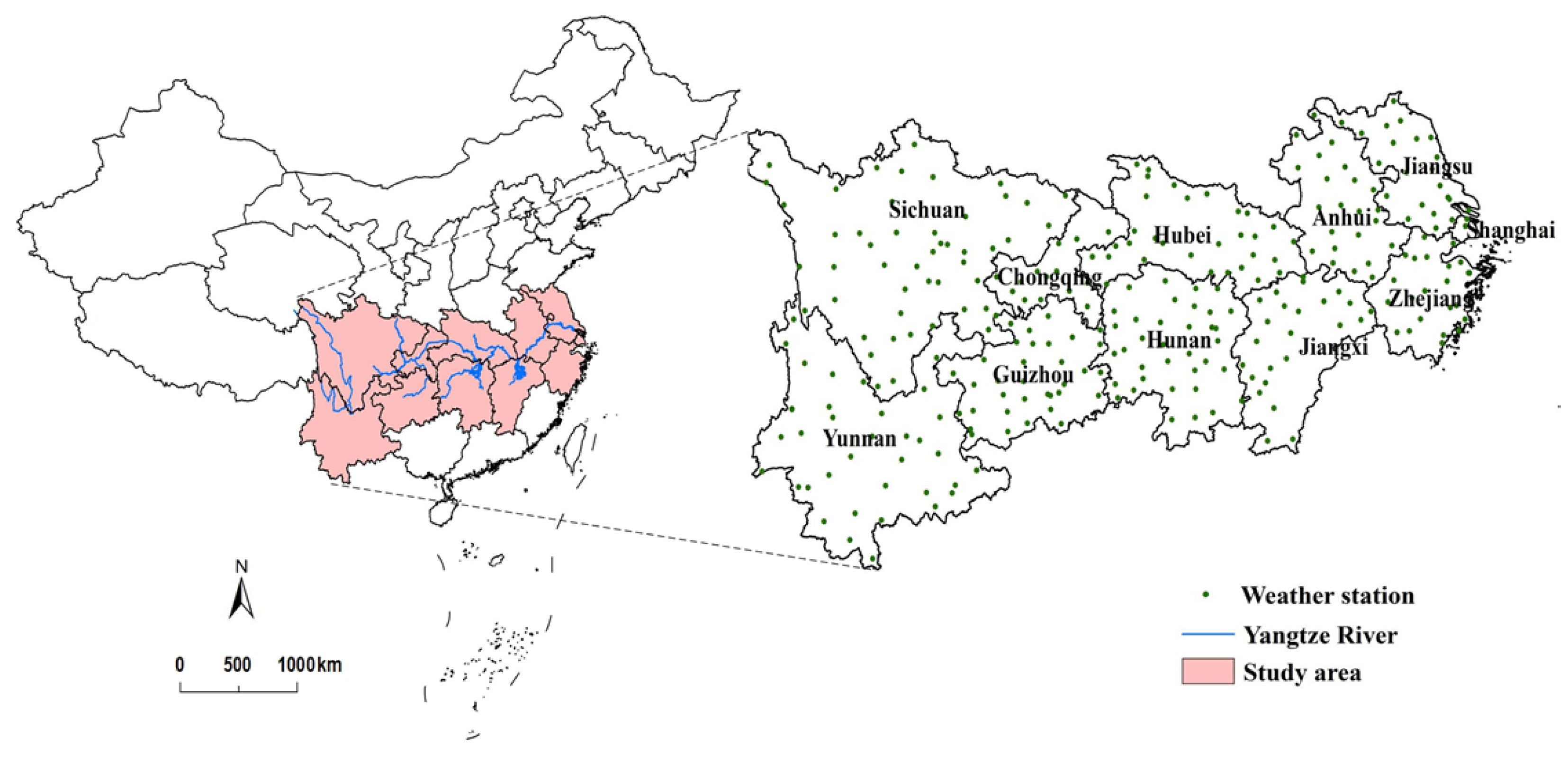
The Yangtze River basin (YRB) is an important agricultural production area in China. It not only produces approximately 40% of the country’s grain, but also maintains a high commodity rate, which plays an important role in balancing the north-south difference in China’s grain pattern. As one of the three core areas of economic development, the basin is also the most obvious area of economic growth and social progress in China. Although precipitation is higher than that in northern China, agricultural non-point source pollution has become one of the major environmental problems in this region due to agricultural technical constraints. The protection of water resources in the Yangtze River basin has been regarded as an important development strategy by China. In this study, 11 provinces and regions of the main stream of the YRB were taken as the objects. The aims of current paper are to: quantify the provincial relationship between agricultural production and water resources from 1999 to 2018 using the water footprint method; analyze the spatial and temporal pattern of AWF and its composition; reveal the driving factors affected AWF variation in the context of social development, using the logarithmic mean divisia index (LMDI) model; and discuss water resource management strategies in the basin based on the research results.
2. Materials and Methods
2.1. Regional Agricultural Water Footprint (AWF) Estimation
The agricultural water footprint (AWF) from crop production in the context of the 11 provinces located in YRB are calculated and analyzed in the current study. The regional AWF is the sum of the water footprint of all crops:
where, n is the number of crops and CWF is the water footprint for a specific crop, in m3. Crops could be categorized as cereals (rice, wheat, corn and other grains), beans, tubers, oil crops (rapeseeds and other oilseeds), cotton, sugar crops (sugarcane and beetroots), fruits and other crops (tea, peanuts, jute, flax and tobacco) in YRB. The CWF is constituted by blue, green and grey components for each kind of crop:
CWFblue, CWFgreen, and CWFgrey are crop blue, green and grey water footprints, respectively, and are estimated according to the methods recommended in the water footprint assessment manual [6]:
A is the crop snow area in ha; Pe and ET are the effective precipitation and field evapotranspiration during the crop cycle in mm; is the leaching-runoff fraction; AR is the rate of nitrogen (N) application to the field, in kg/ha; is the maximum acceptable N concentration in mg L−1; and is the N concentration in natural water, mg L−1.
Pe could be estimated according to empirical formula method recommended by the United State Soil Conservation Service (USDA) [13]:
Pt is the ten-day precipitation during the crop cycle in mm.
ETc was estimated by kthe FAO Penman–Monteith (P-M) method with the aid of the CROPWAT 8.0 model:
where Kc is the crop coefficient, dimensionless; ET0 is the reference evapotranspiration, mm; Δ is the slope of the vapor pressure curve, kPa °C−1; Rn is the net radiation, MJ m−2 d−1; G is the soil heat flux density, MJ m−2 d−1; γ is the psychrometric constant, kPa °C−1; T is the average air temperature, °C; u2 is the wind speed measured at a height of 2 m, m s−1; es is the saturation vapor pressure, kPa; and ea is the actual vapor pressure, kPa.
2.2. Decomposition Analysis of Agricultural Water Footprint
The logarithmic mean Divisia index (LMDI) is currently recognized as a more accurate exponential decomposition method, with a profound theoretical basis and high adaptability [36]. LMDI not only performs multi-factor decomposition, but also overcomes the problem of residual items or the improper decomposition of residual items after decomposition, making the analysis results more convincing [37,38]. In this study, six factors, including water use intensity, economic level, irrigation technique, resources endowment, urbanization degree and population size, were selected as the influencing factors of AWF decomposition in the Yangtze River Basin. The decomposition analysis of AWF can be given by the following equation:
where W is the agricultural water footprint; G refers to the gross agricultural production in CNY; R is the irrigation water withdrawal in m3; A represents the irrigated area, ha; Pr is the rural population; P refers to the total population; i = W/G is the water footprint per unit of gross agricultural production, which represents the water use intensity and can be used to measure agricultural water use efficiency; e = G/R is the gross agricultural production per unit of irrigation water use, which reveals the economic benefits of irrigation; r = R/A is the irrigation water use per unit cropland, indicating the matching of water/land resources and the irrigation technique; t = A/Pr is the per capita irrigated area in rural areas, representing the regional water resources endowment; u = Pr/P is the proportion of the rural population in total, representing the degree of urbanization; and P is the indication of the regional population size.
According to the LMDI method, the general formula for the variation of AWF from the base year to the Tth year can be expressed as:
where WT and W0 are the crop water footprint of the year T and 0, respectively, in Gm3; and ΔWi, ΔWe, ΔWr, ΔWt, ΔWu and ΔWp are the contribution values (including the positive contribution or negative inhibition) of each driving factor to the change of AWF, Gm3. The general formula of each contribution value can be summarized as follows:
where K refers to the driving factors, i, e, r, t, u and p.
2.3. Data Resources
The study areas and time period assessed in the current paper are 11 provinces in the YRB (Figure 1) and the years 1999–2018. Climatic data from 299 weather stations located in the provinces for CROPWAT 8.0 model were obtained from the National Meteorological Information Center of China (http://data.cma.cn/, accessed on 10 March 2021). Yearly irrigation water use (IWU) and irrigation efficiency (IE) for the period 1999–2018 in each province were collected from the China Water Resources Bulletins 1999–2018 (MWR, 1999–2018). The provincial crop yield, sown area gross agricultural production, rural and total population, irrigated area and chemical application to the field were collected from the China Statistical Yearbooks 2000–2019 (NBSC, 2000–2019). AR, Cmax and Cnet are assumed to be 10%, 10 mg L−1 and 0, respectively, referencing previous research [14,16]. A summary for the sources of all of the original data used in this study are listed in Table 1.
3. Results
3.1. AWF and Its Temporal and Spatial Pattern
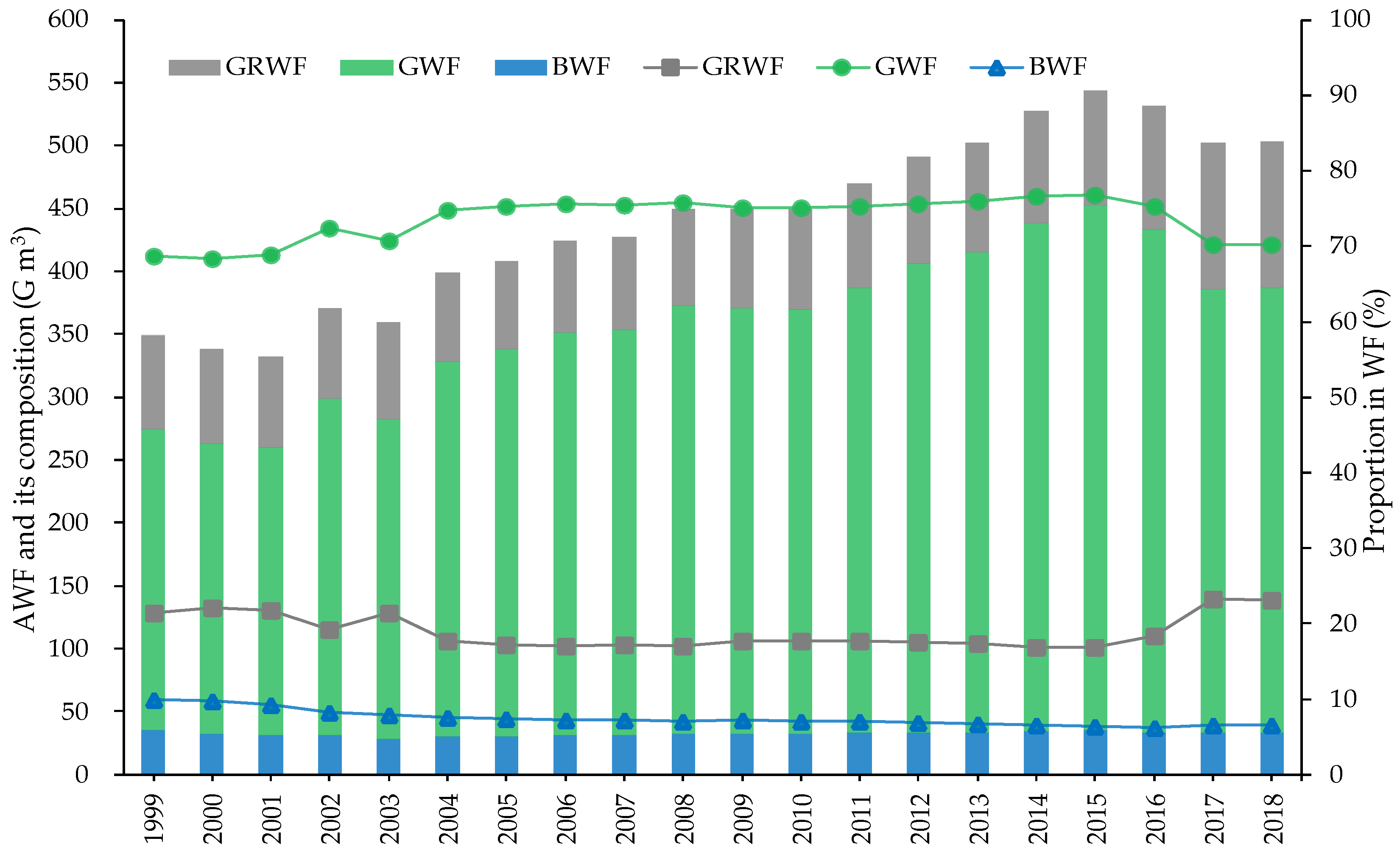
The annual AWF of all the provinces in the YRB during 1999–2018 was 441.6 Gm3, where the blue water footprint (BWF), green water footprint (GWF) and grey water footprint (GRWF) were 32.2, 326.3 and 83.1 Gm3, respectively. The three parts accounted for 7.44%, 73.63%, and 18.93% of the total, respectively. Green water played a dominant role in crop water resource appropriation in the YRB. Figure 2 shows the blue, green, and grey water footprints and their proportions of the AWF in the YRB over the studied period.
With an average growth rate of 1.95% per year, the AWF in the YRB increased from 348.76 Gm3 in 1999 to 503.59 Gm3 in 2018. As shown in Figure 2, the interannual variation trend of AWF could be roughly divided into three stages: stable (1999–2003), increasing (2004–2015) and decreasing (2016–2018) stages. In the first stage, AWF fluctuated around 350 Gm3. In the second stage, the total volume increased rapidly, at a rate of 2.87% per year. The AWF declined year by year in the third stage. Green water was the main source of crop water consumption. With continued increase in crop water demand, green water became the major contributor to increased agricultural water use in the YRB. Clearly, the green water footprint comprised the largest share of the total and remained above 68%. Its inter-yearly variation was essentially consistent with that of the AWF. In addition, the increase in green water consumption led to decrease in the demand on blue water. The blue water footprint remained at 30–35 Gm3 during the research period. However, the proportion of blue water contributing to the total footprint was less than 10%, and continued to decline over time. This proportion decreased from 10% in 1999 to 7% in 2018 due to improvement in irrigation facilities. The proportion of grey water footprint was stable between 17% and 23%, showing a small range of fluctuation. In order to observe the temporal and spatial pattern of provincial crop water use in the YRB, the changes in the AWF in these provinces is given in Table 2.
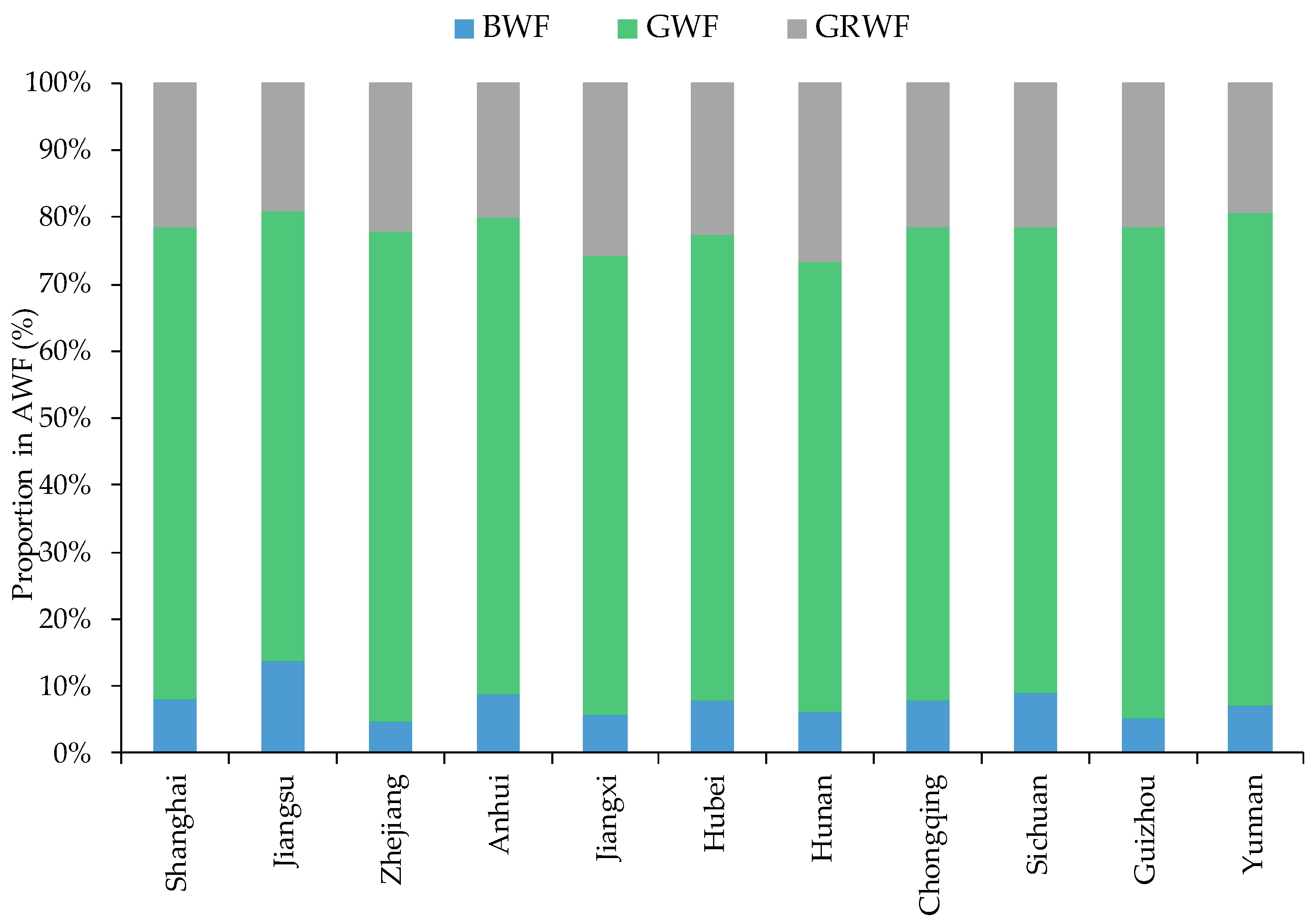
Table 2 reveals that the difference between the minimum value (Shanghai) and the maximum value (Anhui) was 60.46 Gm3. As dominated by the secondary and tertiary industries, Shanghai’s urbanization rate was more than 88%. The effective irrigation area of crops was relatively small, which resulted in the smallest AWF in Shanghai in the whole watershed. The AWF of Anhui and Jiangsu were both above 60 Gm3. As China’s main grain production base, they had a large crop planting area and a great demand for water. In addition, the coefficients of variation in all of the provinces were less than 0.30, with the maximum value of 0.29 in Zhejiang and the minimum of 0.08 in Jiangsu. It was not difficult to find that the provinces with the greatest AWF had a smaller coefficient of variation, which conformed to the law that the coefficient of variation was basically opposite to the spatial distribution pattern of the AWF. The average growth rate of each province was consistent with the variation coefficient. In other words, the annual growth rate of provinces with low coefficients of variation were low. In Shanghai, Jiangsu, Anhui and Sichuan the growth rate was less than 2 percent per year. Among the remaining seven provinces, Zhejiang had the highest annual growth rate, at 3.54%. In order to further understand the consumption of different types of water resources, Figure 3 provides the annual proportion of blue, green and grey water footprints in the AWF for each province.
During the research period, the annual blue, green and grey water footprints of the YRB were estimated to be 7.61, 70.46 and 21.92 Gm3, respectively. The green water (rain water) of all provinces occupied an absolute dominant position, and the blue water (irrigation) only accounted for about 1/10 in the YRB. Taking the stem stream of the Yangtze River as the boundary, we divided the 11 provinces into two regions: the above Yangtze River (Shanghai, Jiangsu, Anhui, Hubei, Chongqing and Sichuan) and the below Yangtze River (Zhejiang, Jiangxi, Hunan, Guizhou and Yunnan). The overall observation showed that the blue water footprint proportion in the above Yangtze River regions was higher than that in the below Yangtze River regions. The grey water footprint in the above Yangtze River regions (except Yunnan) was smaller than that in the below Yangtze River regions. Anhui and Jiangsu were the regions with high agricultural production level and grain output in China. With lower annual rainfall than the southeast provinces, Anhui and Jiangsu needed to replenish a large amount of irrigation water to meet crop needs. This was the reason for their relatively high blue water footprint. Figure 3 shows that the proportion of the grey water footprint in Hunan and Jiangxi was more than 25%. For a long time, Hunan and Jiangxi had prominent water environment problems, and they were the concentrated places of non-point source pollution in China. To dilute pollutants in order to achieve the level of concentration allowed by the environment, a large amount of water resources were consumed, with the result that their grey water footprint was significantly higher than in other provinces.
3.2. Distribution and Composition of AWF in YRB
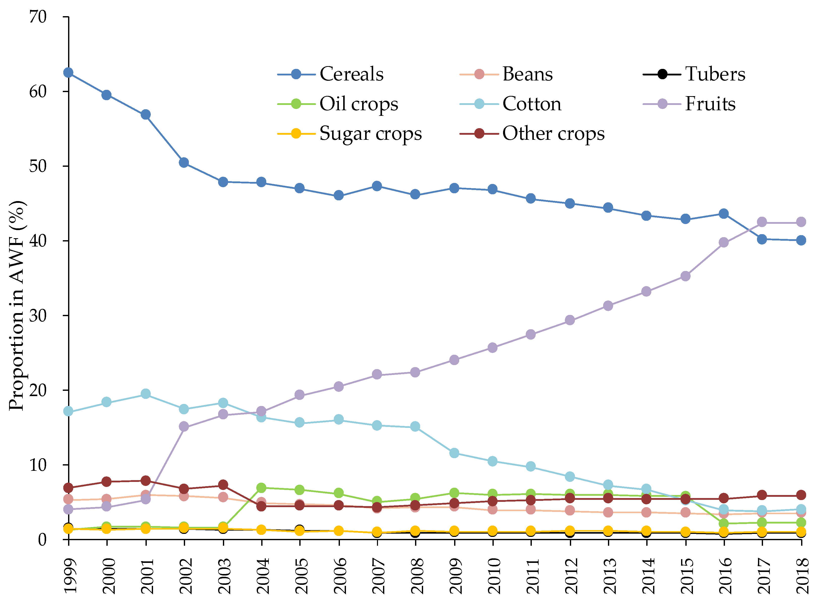
Cereals, beans and tubers were collectively referred to as grain crops, and oil crops, cotton, sugar crops, fruits and other crops were collectively referred to as cash crops. In order to observe the water consumption of different types of crops in agricultural production, Figure 4 shows the changing trend of the water footprint ratio of eight categories of crops over the observed period.
According to Figure 4, the proportion of AWF in the research period could be divided into three stages. Phase I (1999–2001): during which the combined water footprint of grain and cotton accounted for more than 76% of the total AWF, reaching 79.5% in 1999. The water requirement per unit area of cereals and cotton was 600–700 mm, and around 400 mm for other crops. The proportion of cereals decreased rapidly, while that of cotton increased slightly, both of which dominated the trend of the AWF in the YRB. Phase II (2002–2016): during which cereals were still the crop with the largest proportion in AWF, which was always stable at more than 42%. Fruit had overtaken cotton as the crop contributing the second largest amount to the AWF. The proportion of fruit in the AWF was growing rapidly in this sub-period, increasing by nearly 25% in 2016 compared to 2004. In contrast, low productivity and rising labor costs reduced the cotton share by 13.5 percent. Phase III (2017–2018): during which the water footprint of cereals decreased with time and the water footprint of fruits increases rapidly. Fruits became the crop with greatest water footprint in 2017. At this time, cereals and fruits jointly accounted for about 45% of the AWF. According to the above analysis, the changing trend of the AWF was mainly affected by cereals, cotton and fruits. None of the proportions of beans, tubers, oil crops, sugar crops and other crops in the studied period exceeded 10%. The proportion of these crops varied slightly and had little impact on the temporal and spatial distribution of the AWF. The crops that changed significantly during the research were cotton, fruits and grains. At the beginning of the 20th century, the YRB was economically backward, and food and clothing became a national necessity. Cereals and cotton were planted with a large area and high yield, and the AWF was correspondingly large, which was in line with the national conditions at that time. With development of the economy, changes in market demand prompted farmers to keenly produce fruits with higher economic value. Optimizing the planting structure and planting cash crops on a large scale were of great significance to the development of modern agriculture. Figure 5 shows the annual AWF composition structure of eight crops in each province over the period of 1999–2018.
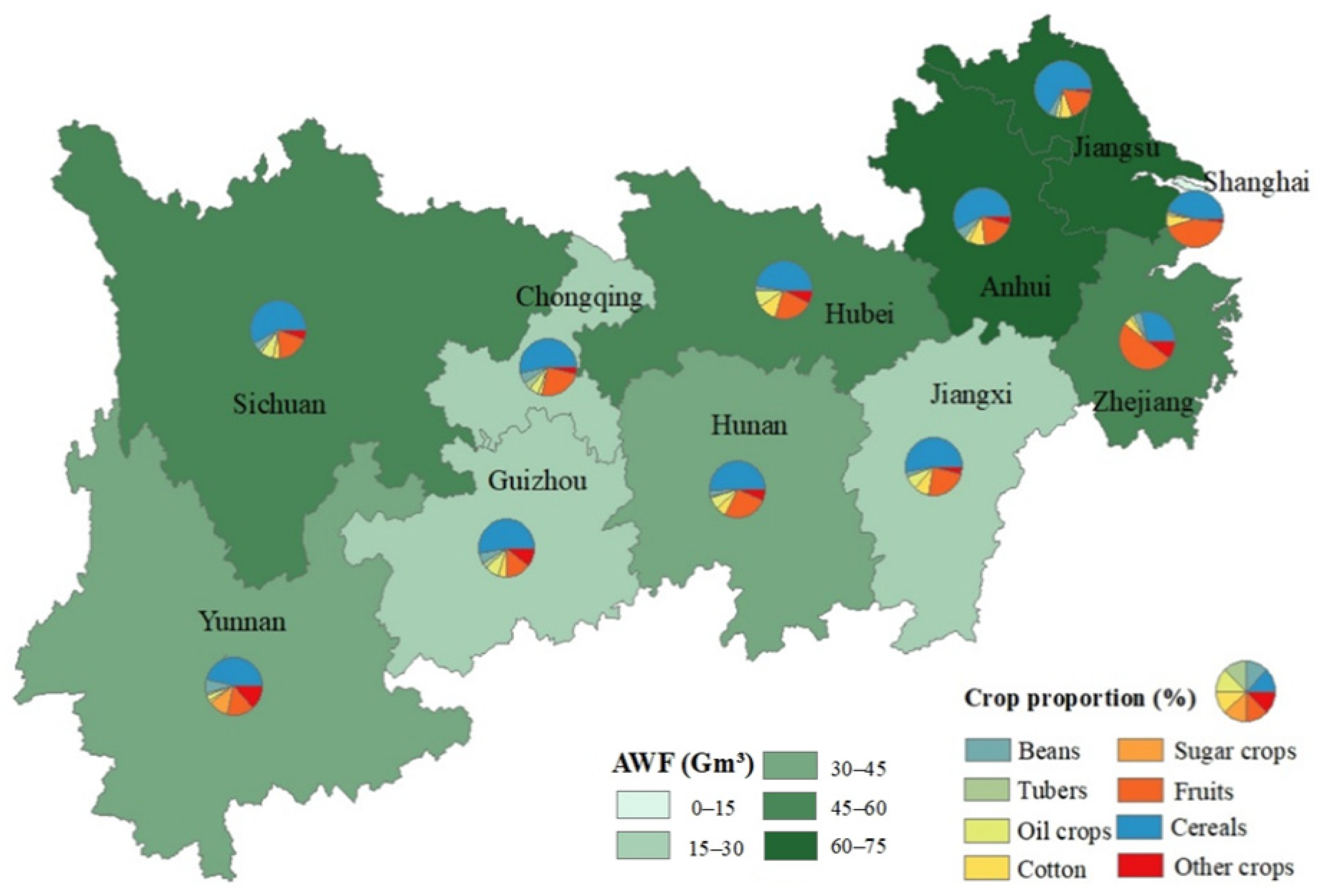
Figure 5 shows the annual AWF and crop composition in each province in order to observe the spatial distribution of water use. It can be seen from the figure that Jiangsu and Anhui had the greatest water footprint, while Shanghai had the smallest. The water footprint of most provinces was still dominated by grain crops. In Jiangsu, Anhui and Sichuan, grain crops accounted for more than 65% of the AWF, of which cereals accounted for about 58%. Cereals per unit area required a large amount of water. The sowing area of cereals in Chongqing and Guizhou was small, which directly led to their small AWF. On the other hand, only Shanghai and Zhejiang were dominated by cash crops, accounting for 53% and 66%, respectively. The per capita arable land resources in Shanghai and Zhejiang were lower than the national level. The acceleration of industrialization and urbanization had intensified tensions around land resources. The increasingly acute contradiction between people and land forced the transformation of cultivated land use types and crop planting patterns. More and more farmers favored high-yield cash crops. In addition, large amounts of chemical fertilizer application and serious non-point source pollution in Zhejiang resulted in a high grey water footprint, which increased the AWF in Zhejiang. It is worth noting that the grain output of Jiangxi and Yunnan was similar, but Yunnan’s AWF was higher than that of Jiangxi. Because other crops accounted for a relatively large proportion in Yunnan, especially the tobacco industry and tea industry which were key pillar industries, and these cash crops contributed a large water footprint.
3.3. Driving Factors of AWF
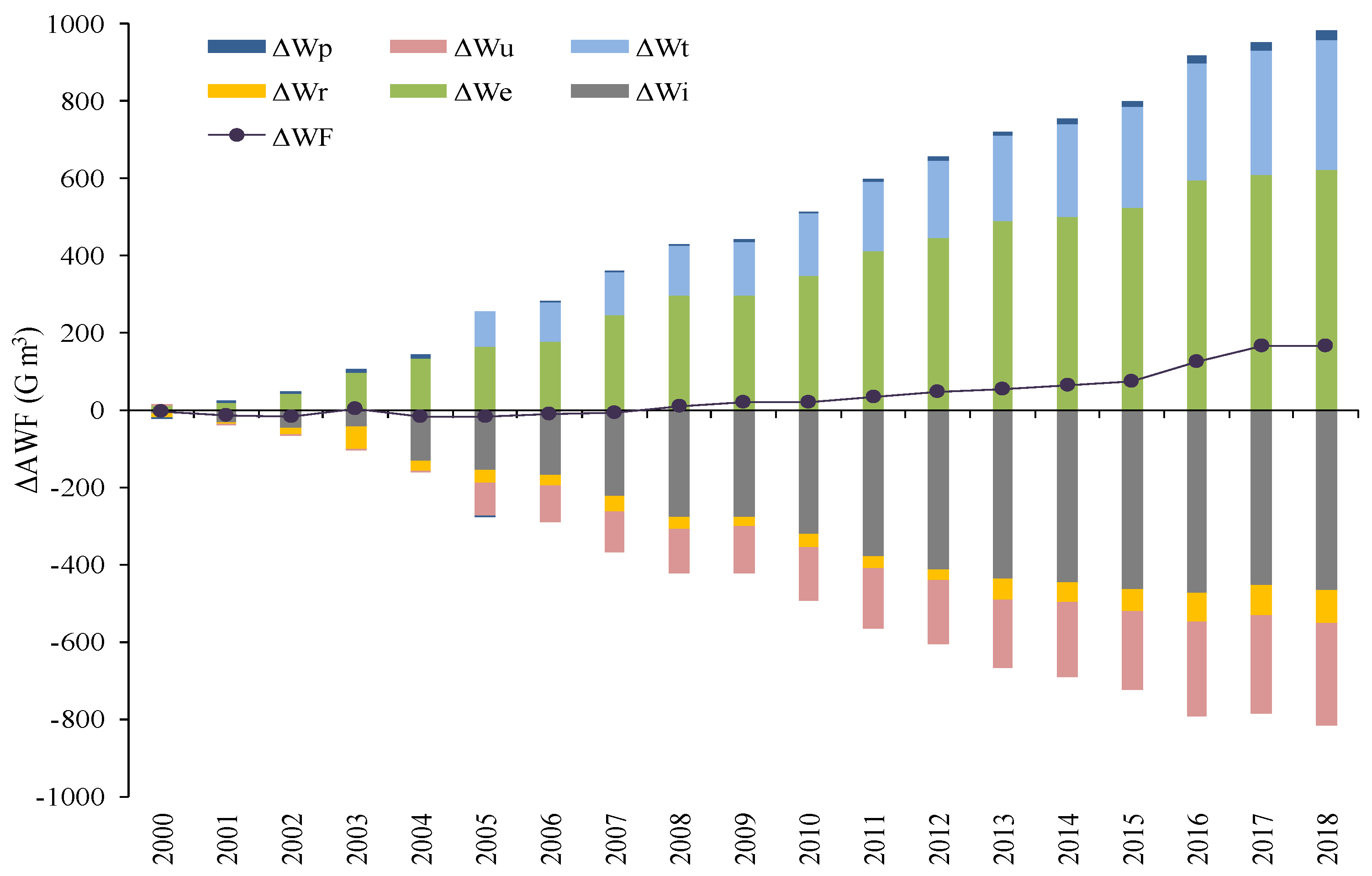
The annual value of the ΔWF in the YRB was 36.52 Gm3, indicating that the agricultural water consumption increased over the past 20 years. The annual values of the selected six factors (ΔWi, ΔWe, ΔWr, ΔWt, ΔWu, and ΔWp) were calculated to be −274.25, 317.53, −39.19, 148.02, −123.39 and 8.59 Gm3, respectively. Figure 6 shows the analysis results of factors affecting AWF changes over time.
The ΔAWF generally increased year by year, taking 1999 as the base year. From 2000 to 2007, the ΔAWF was slightly less than 0 and relatively stable, which meant that the AWF had not changed much during this period. From 2008 to 2018, the ΔAWF increased rapidly, with a growth rate of 33.4% per year. Rapid economic development and the expansion of crop planting areas played a decisive role in 2008–2018. As shown in Figure 6, the contributing factors to the AWF included economic level (ΔWe), resources endowment (ΔWt) and population size (ΔWp), and the inhibiting factors were water use intensity (ΔWi), irrigation technology (ΔWr) and urbanization degree (ΔWu). Among all of the factors, ΔWe had the greatest influence on changes to the AWF. In 2018, the value of ΔWe reached up to 623.73 Gm3, which was twice that of the contributing factor ΔWt and 25 times that of ΔWp. With an annual growth rate of 24.8%, ΔWe stimulated the AWF to increase by 612.1 Gm3 during the whole research period. As the most restrictive factor, ΔWi maintained an opposite driving effect to ΔWe. The effect of ΔWt and ΔWu on the AWF was slightly weaker than that of ΔWe and ΔWi. The factor of ΔWr had the smallest inhibitory effect among the three inhibitory factors. The inhibitory effect of was about one-seventh that of ΔWi. The factor of ΔWp increased from 0.9 Gm3 in 1999 to 24.6 Gm3 in 2018, which was the smallest effect and change range among all of the influencing factors. The effect of the regional population size on the increase of the AWF was almost negligible. As the spatial distribution pattern of the AWF was generally stable in different years, the annual value of ΔAWF and its composition in 20 years was calculated in order to analyze the influencing factors of the spatial distribution. The results are shown in Table 3.
The average value of ΔAWF for 11 provinces over the past 20 years was 3.39 Gm3, which was greatly influenced by ΔWi and ΔWe. There were significant differences in the driving factors among the different provinces. According to Table 3, all of the ΔAWF was greater than 0, except for Shanghai and Jiangsu. The ΔAWF in Anhui, Hubei, Hunan and Yunnan exceeded 5 Gm3, indicating that agricultural water use was high in these provinces. Shanghai has the smallest water footprint and influencing factors in the basin due to its very small crop planting area. The most important factor for inhibiting the growth of the AWF was ΔWi. The inhibition effects of the water footprint per unit of gross agricultural production in Jiangsu, Anhui, Hubei and Sichuan were higher than that in other provinces. Jiangsu was the only province with a ΔAWF of no more than 0 among these four provinces, indicating that its water resource utilization efficiency was greatly improved. The implementation of water-control policies played an important role in water-saving, to a certain extent. In addition, the inhibitory effect of ΔWu in Jiangsu could not be underestimated. Its contribution value was more than 10 Gm3 and was higher than that of the other three provinces. Moreover, ΔWe contributed to water consumption in all provinces. The contribution value of the economic level in Hubei was 51.89 Gm3, which was the maximum value among the 11 provinces. This showed that Hubei’s rapid economic growth came at the cost of abundant water resources. The ΔWp in Hubei was −0.76 Gm3, and the population loss reduced the AWF in this province. Some provinces with large population losses showed a slight inhibitory effect, although ΔWp was a contributing factor to the AWF in YRB. The minimum value of ΔWe appeared in Shanghai, because its economic structure mostly depended on secondary and tertiary industries. In addition, ΔWr was largely a restrictive factor, showing a contribution in only a few provinces. The strongest inhibition and contribution effects in Hubei and Jiangsu were due to ΔWr. This indicated that modern agricultural irrigation technology in Hubei was more advanced than that in Jiangsu. Furthermore, ΔWt contributed to ΔAWF in all provinces. The difference between the maximum value in Anhui (27.74 Gm3) and the minimum value in Shanghai (0.25 Gm3) was 27.49 Gm3. The ΔWt of Jiangsu, Anhui and Sichuan all exceeded 20 Gm3. These regions were rich in water and land resources, which contributed the majority of the AWF in the YRB. Despite great variation, ΔWu showed inhibitory effects on all provinces. For example, the ΔWu in Jiangsu was as high as −29.62 Gm3, while it is only −3.54 Gm3 in Guizhou. Compared with other factors, the contribution value of ΔWp in all of provinces had little difference and fluctuated between −2~5 Gm3. The ΔWp for the whole YRB was greater than 0, while both positive and negative values could be found at the provincial scale. Provinces with large population inflow showed a contribution effect, and provinces with serious population loss showed a slight inhibition effect. For instance, Jiangsu and Zhejiang were the provinces with largest net inflow of population, which led to the largest contribution to the population scale. Anhui, Hubei and Sichuan had considerable population loss, and their ΔWp was slightly less than 0. In general, whether it was a contribution or an inhibitory effect, the influence of ΔWp on AWF was always minimal.
4. Discussion
Beyond the natural factors, this paper attempted to analyze the relationship between the AWF and elements which reflect social evolution. The results of this study provides references for regional water footprint regulation and agricultural water management from a new perspective. As an economic zone with large population, strong comprehensive strength, important ecological status and sufficient development potential, the YRB has played an important strategic supporting role in coordinating regional development, cultivating growth momentum and optimizing spatial structure for a long time. Covering 11 provinces, the YRB spans China’s eastern, central and western regions. There are significant differences in economic and social development among these provinces. Agricultural water use in the YRB is representative, and the agricultural water management based on its water footprint regulation plays an enlightening role throughout the world. Based on the advanced function of the LMDI and a large number of calculations and analysis, we find our results to be reliable. This is meaningful for water resource management policy formulation. Some suggestions based on our findings are as follows. In relation to the main grain-producing regions, we suggest: maintaining the current grain production level to ensure national food security; actively guiding the change of grain production mode and promoting the cultivation and quality of grain varieties; and reducing the AWF and increasing farmers’ incomes by adjusting crop composition appropriately. In relation to the areas with a developed economy that does not rely on agriculture, we suggest that: the developed economy is obtained at the expense of the ecological environment; high agricultural production risk, low water use efficiency and frequent environmental incidents hindered the further development of these areas; insufficient attention to agriculture has resulted in limited space for agricultural development., and therefore, it is particularly important to promote the high-quality and high-efficiency development of modern agriculture; it is feasible to strengthen the construction of well-known agricultural brand, improve the level of irrigation technology and optimize the use of water and land resources. In relation to the areas with a backward economy and low agricultural water efficiency, we suggest: adjusting the crop planting structure and increasing the proportion of cash crops to reduce agricultural water use and achieve higher economic benefits; focusing on improvement and innovation in agricultural water-saving technologies and strengthening the promotion of water-saving technologies to improve irrigation efficiency; establishing a sound water resource management system and optimizing water resource allocation; strengthening urbanization to increase the rate of urbanization. Finally, in relation to the areas with serious non-point source pollution, we suggest that: severe agricultural non-point source pollution has brought a high grey water footprint; non-point source pollution is a comprehensive and systematic project involving economic and social development, industrial structural adjustment and ecological environment management. The following measures can be taken to reduce non-point source pollution: controlling agricultural non-point source pollution and speeding up the comprehensive improvement of the rural environment; deepening the prevention and control of pollution in key river basins and regions in order to strengthen water resource protection; applying pesticides and fertilizers scientifically, and promoting organic agriculture and ecological agriculture. Finally, strengthening exchanges and cooperation among different regions and learning from each other’s advanced experience and technology in order to achieve sustainable development.
5. Conclusions
This paper analyzed the temporal and spatial differences of crop water footprints and their structures, and revealed the driving mechanism of agricultural water use in the YRB based on the LMDI model. The conclusions were as follows. The agricultural water consumption in the YRB increased by 154.83 Gm3 during the research period, where the green water footprint occupied an absolute dominant position. The provinces with the large water appropriation were Jiangsu, Anhui, Hubei and Sichuan. The total AWF of the four provinces accounted for 54% in the YRB, which matched their status as major grain cultivating provinces. The AWF of cereals and fruits jointly accounted for more than 82%, and dominated the trend of AWF. Economic level and water use intensity were the largest contributors and inhibitors that changed the AWF, respectively. The driving effect of each factor varied significantly among provinces. Economic level and water use intensity had the most prominent effect on Jiangsu, Anhui, Hubei and Sichuan. Maintaining the balance between economic development and water resource protection in the Yangtze River Basin has a long way to go. This study provides reliable theoretical support and policy inspiration for achieving this goal. It is necessary to further explore the relationship between water resource systems and agricultural production in order to achieve the goals of global food security and water conservation in the future.
Author Contributions
Conceptualization, W.Z. and X.C.; methodology, W.Z. and X.C.; software, W.Z. and J.H.; validation, W.Z., X.C., J.H. and Y.Q.; formal analysis, W.Z. and Y.Q.; investigation, W.Z., Y.Q. and X.C.; resources, X.C.; data curation, W.Z. and X.C.; writing—original draft preparation, W.Z. and X.C.; writing—review and editing, W.Z., X.C. and J.H.; visualization, J.H.; supervision, X.C.; project administration, X.C.; funding acquisition, X.C. All authors have read and agreed to the published version of the manuscript.
Funding
National Natural Science Foundation of China (51979074) and the Fundamental Research Funds for the Central Universities (B200202095, B210203152).
Institutional Review Board Statement
Not applicable.
Informed Consent Statement
Not applicable.
Data Availability Statement
Not applicable.
Acknowledgments
This work is jointly funded by National Natural Science Foundation of China (51979074) and the Fundamental Research Funds for the Central Universities (B200202095, B210203152).
Conflicts of Interest
The authors declare no conflict of interest.
References
- Cao, X.; Zeng, W.; Wu, M.; Li, T.; Chen, S.; Wang, W. Water resources efficiency assessment in crop production from the perspective of water footprint. J. Clean. Prod. 2021, 309, 127371. [Google Scholar] [CrossRef]
- Mekonnen, M.M.; Gerbens-Leenes, W. The water footprint of global food production. Water 2020, 12, 2696. [Google Scholar] [CrossRef]
- Cao, X.; Wu, M.; Guo, X.; Zheng, Y.; Gong, Y.; Wu, N.; Wang, W. Assessing water scarcity in agricultural production system based on the generalized water resources and water footprint framework. Sci. Total Environ. 2017, 609, 587–597. [Google Scholar]
- Long, A.; Zhang, P.; Hai, Y.; Deng, X.; Li, J.; Wang, J. Spatio-Temporal Variations of Crop Water Footprint and Its Influencing Factors in Xinjiang, China during 1988–2017. Sustainability 2020, 12, 9678. [Google Scholar] [CrossRef]
- Cao, X.; Zeng, W.; Wu, M.; Guo, X.; Wang, W. Hybrid analytical framework for regional agricultural water resource utilization and efficiency evaluation. Agric. Water Manag. 2020, 231, 106027. [Google Scholar] [CrossRef]
- Aldaya, M.M.; Chapagain, A.K.; Hoekstra, A.Y.; Mekonnen, M.M. The Water Footprint Assessment Manual: Setting the Global Standard; Routledge: London, UK, 2012. [Google Scholar]
- Hoekstra, A.Y.; Mekonnen, M.M. The water footprint of humanity. Proc. Natl. Acad. Sci. USA 2012, 109, 3232–3237. [Google Scholar] [CrossRef] [PubMed] [Green Version]
- Bazrafshan, O.; Dehghanpir, S. Application of water footprint, virtual water trade and water footprint economic value of citrus fruit productions in Hormozgan Province, Iran. Sustain. Water Resour. Manag. 2020, 6, 1–10. [Google Scholar] [CrossRef]
- Matohlang Mohlotsane, P.; Owusu-Sekyere, E.; Jordaan, H.; Barnard, J.H.; Van Rensburg, L.D. Water footprint accounting along the wheat-bread value chain: Implications for sustainable and productive water use benchmarks. Water 2018, 10, 1167. [Google Scholar] [CrossRef] [Green Version]
- Aldaya, M.M.; Martínez-Santos, P.; Llamas, M.R. Incorporating the water footprint and virtual water into policy: Reflections from the Mancha occidental region, Spain. Water Resour. Manag. 2010, 24, 941–958. [Google Scholar] [CrossRef] [Green Version]
- Dong, H.; Geng, Y.; Fujita, T.; Fujii, M.; Hao, D.; Yu, X. Uncovering regional disparity of china’s water footprint and inter-provincial virtual water flows. Sci. Total Environ. 2014, 500–501, 120–130. [Google Scholar] [CrossRef]
- Fader, M.; Gerten, D.; Thammer, M.; Heinke, J.; Lotze-Campen, H.; Lucht, W.; Cramer, W. Internal and external green-blue agricultural water footprints of nations, and related water and land savings through trade. Hydrol. Earth Syst. Sci. 2011, 15, 1641–1660. [Google Scholar] [CrossRef] [Green Version]
- Cao, X.C.; Wu, P.T.; Wang, Y.B.; Zhao, X.N. Assessing blue and green water utilisation in wheat production of China from the perspectives of water footprint and total water use. Hydrol. Earth Syst. Sci. 2014, 18, 3165–3178. [Google Scholar] [CrossRef] [Green Version]
- Mekonnen, M.M.; Hoekstra, A.Y. The green, blue and grey water footprint of crops and derived crop products. Hydrol. Earth Syst. Sci. 2011, 15, 1577–1600. [Google Scholar] [CrossRef] [Green Version]
- Lovarelli, D.; Bacenetti, J.; Fiala, M. Water footprint of crop productions: A review. Sci. Total Environ. 2016, 236, 548–549. [Google Scholar] [CrossRef]
- Zhuo, L.; Mekonnen, M.M.; Hoekstra, A.Y. Benchmark levels for the consumptive water footprint of crop production for different environmental conditions: A case study for winter wheat in China. Hydrol. Earth Syst. Sci. 2016, 20, 4547–4559. [Google Scholar] [CrossRef] [Green Version]
- Ewaid, S.H.; Abed, S.A.; Al-Ansari, N. Water Footprint of Wheat in Iraq. Water 2019, 11, 535. [Google Scholar] [CrossRef] [Green Version]
- Muratoglu, A. Water footprint assessment within a catchment: A case study for Upper Tigris River Basin. Ecol. Indic. 2019, 106, 105467. [Google Scholar] [CrossRef]
- Han, Y.; Jia, D.; Zhuo, L.; Sauvage, S.; Sánchez-Pérez, J.M.; Huang, H.; Wang, C. Assessing the water footprint of wheat and maize in Haihe River Basin, Northern China (1956–2015). Water 2018, 10, 867. [Google Scholar] [CrossRef] [Green Version]
- Chu, Y.; Shen, Y.; Yuan, Z. Water footprint of crop production for different crop structures in the Hebei southern plain, North China. Hydrol. Earth Syst. Sci. 2017, 21, 3061–3069. [Google Scholar] [CrossRef] [Green Version]
- Xu, Z.; Chen, X.; Wu, S.R.; Gong, M.; Du, Y.; Wang, J.; Liu, J. Spatial-temporal assessment of water footprint, water scarcity and crop water productivity in a major crop production region. J. Clean. Prod. 2019, 224, 375–383. [Google Scholar] [CrossRef]
- Safitri, L.; Hermantoro, H.; Purboseno, S.; Kautsar, V.; Saptomo, S.K.; Kurniawan, A. Water footprint and crop water usage of oil palm (Eleasis guineensis) in Central Kalimantan: Environmental sustainability indicators for different crop age and soil conditions. Water 2019, 11, 35. [Google Scholar] [CrossRef] [Green Version]
- Vale, R.L.; Netto, A.M.; de Lima Xavier, B.T.; Barreto, M.D.L.P.; da Silva, J.P.S. Assessment of the gray water footprint of the pesticide mixture in a soil cultivated with sugarcane in the northern area of the State of Pernambuco, Brazil. J. Clean. Prod. 2019, 234, 925–932. [Google Scholar] [CrossRef]
- Luan, X.B.; Yin, Y.L.; Wu, P.T.; Sun, S.K.; Wang, Y.B.; Gao, X.R.; Liu, J. An improved method for calculating the regional crop water footprint based on a hydrological process analysis. Hydrol. Earth Syst. Sci. 2018, 22, 5111–5123. [Google Scholar] [CrossRef] [Green Version]
- Xinchun, C.; Mengyang, W.; Rui, S.; La, Z.; Dan, C.; Guangcheng, S.; Shuhai, T. Water footprint assessment for crop production based on field measurements: A case study of irrigated paddy rice in East China. Sci. Total Environ. 2018, 610, 84–93. [Google Scholar] [CrossRef]
- Wu, M.; Cao, X.; Ren, J.; Shu, R.; Zeng, W. Formation mechanism and step effect analysis of the crop gray water footprint in rice production. Sci. Total Environ. 2021, 752, 141897. [Google Scholar] [CrossRef] [PubMed]
- Zheng, J.; Wang, W.; Ding, Y.; Liu, G.; Xing, W.; Cao, X.; Chen, D. Assessment of climate change impact on the water footprint in rice production: Historical simulation and future projections at two representative rice cropping sites of China. Sci. Total Environ. 2020, 709, 136190. [Google Scholar] [CrossRef] [PubMed]
- Yang, M.; Xiao, W.; Zhao, Y.; Li, X.; Huang, Y.; Lu, F.; Li, B. Assessment of potential climate change effects on the rice yield and water footprint in the Nanliujiang catchment, China. Sustainability 2018, 10, 242. [Google Scholar] [CrossRef] [Green Version]
- Ahmadi, M.; Etedali, H.R.; Elbeltagi, A. Evaluation of the effect of climate change on maize water footprint under RCPs scenarios in Qazvin plain, Iran. Agric. Water Manag. 2021, 254, 106969. [Google Scholar] [CrossRef]
- Huang, H.; Han, Y.; Jia, D. Impact of climate change on the blue water footprint of agriculture on a regional scale. Water Supply 2019, 19, 52–59. [Google Scholar] [CrossRef] [Green Version]
- Wu, M.; Cao, X.; Guo, X.; Xiao, J.; Ren, J. Assessment of grey water footprint in paddy rice cultivation: Effects of field water management policies. J. Clean. Prod. 2021, 313, 127876. [Google Scholar] [CrossRef]
- Cao, X.; Shu, R.; Ren, J.; Wu, M.; Huang, X.; Guo, X. Variation and driving mechanism analysis of water footprint efficiency in crop cultivation in China. Sci. Total Environ. 2020, 572, 138537. [Google Scholar] [CrossRef] [PubMed]
- Chukalla, A.D.; Krol, M.S.; Hoekstra, A.Y. Green and blue water footprint reduction in irrigated agriculture: Effect of irrigation techniques, irrigation strategies and mulching. Hydrol. Earth Syst. Sci. 2015, 19, 4877–4891. [Google Scholar] [CrossRef] [Green Version]
- Zhang, P.; Deng, X.; Long, A.; Hai, Y.; Li, Y.; Wang, H.; Xu, H. Impact of Social Factors in Agricultural Production on the Crop Water Footprint in Xinjiang, China. Water 2018, 10, 1145. [Google Scholar] [CrossRef] [Green Version]
- Aznar-Sánchez, J.A.; Belmonte-Ureña, L.J.; Velasco-Muñoz, J.F.; Manzano-Agugliaro, F. Economic analysis of sustainable water use: A review of worldwide research. J. Clean. Prod. 2018, 198, 1120–1132. [Google Scholar] [CrossRef]
- Dong, K.; Jiang, H.; Sun, R. Driving forces and mitigation potential of global CO2 emissions from 1980 through 2030: Evidence from countries with different income levels. Sci. Total Environ. 2018, 649, 335–343. [Google Scholar] [CrossRef] [PubMed]
- Hasan, M.; Wu, C. Estimating energy-related CO2 emission growth in bangladesh: The lmdi decomposition method approach. Energy Strategy Rev. 2020, 32, 100565. [Google Scholar] [CrossRef]
- Tursun, H.; Li, Z.; Liu, R.; Li, Y.; Wang, X. Contribution weight of engineering technology on pollutant emission reduction based on IPAT and LMDI methods. Clean Technol. Environ. Policy 2015, 17, 225–235. [Google Scholar] [CrossRef]
Figure 1.
Location of the study area in weather stations.

Figure 2.
AWF and its composition in the YRB from 1999 to 2018.

Figure 3.
Composition of AWF in each province of the YRB.

Figure 4.
Crop species structure of AWF in the YRB.

Figure 5.
Spatial distribution of AWF in the YRB.

Figure 6.
Results of factor decomposition from 1999 to 2018.


Table 1.
Summary for the sources of all the original data used in current study.
| Type of Data | Parameters | Stations/Regions | Source |
|---|---|---|---|
| Meteorological data | maximum temperature, minimum temperature, relative humidity, wind speed, sunshine hours and precipitation | 299 weather stations | National Meteorological Information Center of China (http://data.cma.cn/ accessed on 10 March 2021) |
| Water resources data | irrigation water use (IWU) and irrigation efficiency (IE) | 11 provinces | China Water Resources Bulletins 1999–2018 |
| Statistical data | crop yield, sown area, gross agricultural production, rural and total population, irrigated area and chemical application | 11 provinces | China Statistical Yearbooks 2000–2019 |
Table 2.
Main statistical parameters of AWF in provinces from 1999 to 2018.
| Regions | AWF (Gm3) | Coefficient of Variation | Average Growth Rate (%) |
|---|---|---|---|
| Shanghai | 8.25 | 0.22 | 1.19 |
| Jiangsu | 61.49 | 0.08 | 0.63 |
| Zhejiang | 45.66 | 0.29 | 3.54 |
| Anhui | 68.71 | 0.10 | 1.41 |
| Jiangxi | 24.68 | 0.18 | 2.40 |
| Hubei | 53.33 | 0.20 | 2.78 |
| Hunan | 42.00 | 0.18 | 2.89 |
| Chongqing | 29.59 | 0.20 | 2.94 |
| Sichuan | 55.00 | 0.14 | 1.84 |
| Guizhou | 18.58 | 0.17 | 2.11 |
| Yunnan | 34.28 | 0.20 | 2.63 |
Table 3.
Analysis of the spatial difference of ΔAWF and its composition in various provinces.
| Regions | ΔWF | ΔWi | ΔWe | ΔWr | ΔWt | ΔWu | ΔWp |
|---|---|---|---|---|---|---|---|
| Shanghai | −0.61 | −1.50 | 1.19 | 0.50 | 0.25 | −2.15 | 1.10 |
| Jiangsu | −2.27 | −52.52 | 42.89 | 7.16 | 25.54 | −29.62 | 4.29 |
| Zhejiang | 2.34 | −11.40 | 19.66 | −6.34 | 9.21 | −11.87 | 3.08 |
| Anhui | 6.28 | −34.98 | 40.95 | −9.14 | 27.74 | −17.56 | −0.74 |
| Jiangxi | 3.68 | −15.96 | 20.18 | −0.74 | 5.30 | −6.13 | 1.03 |
| Hubei | 5.86 | −41.23 | 51.89 | −10.62 | 18.64 | −12.06 | −0.76 |
| Hunan | 7.11 | −24.33 | 35.50 | −6.30 | 13.97 | −12.15 | 0.42 |
| Chongqing | 2.55 | −10.52 | 11.38 | 0.67 | 8.55 | −7.06 | −0.47 |
| Sichuan | 3.28 | −43.45 | 45.85 | −3.01 | 20.12 | −14.52 | −1.71 |
| Guizhou | 0.89 | −16.03 | 15.40 | −4.53 | 9.88 | −3.54 | −0.29 |
| Yunnan | 8.20 | −22.35 | 32.64 | −6.84 | 8.82 | −6.74 | 2.65 |
Publisher’s Note: MDPI stays neutral with regard to jurisdictional claims in published maps and institutional affiliations. |
© 2021 by the authors. Licensee MDPI, Basel, Switzerland. This article is an open access article distributed under the terms and conditions of the Creative Commons Attribution (CC BY) license (https://creativecommons.org/licenses/by/4.0/).
Share and Cite
MDPI and ACS Style
Zeng, W.; He, J.; Qiu, Y.; Cao, X. Unravelling the Temporal-Spatial Distribution of the Agricultural Water Footprint in the Yangtze River Basin (YRB) of China. Water 2021, 13, 2562. https://doi.org/10.3390/w13182562
AMA Style
Zeng W, He J, Qiu Y, Cao X. Unravelling the Temporal-Spatial Distribution of the Agricultural Water Footprint in the Yangtze River Basin (YRB) of China. Water. 2021; 13(18):2562. https://doi.org/10.3390/w13182562
Chicago/Turabian StyleZeng, Wen, Junchen He, Yaliu Qiu, and Xinchun Cao. 2021. "Unravelling the Temporal-Spatial Distribution of the Agricultural Water Footprint in the Yangtze River Basin (YRB) of China" Water 13, no. 18: 2562. https://doi.org/10.3390/w13182562
Note that from the first issue of 2016, this journal uses article numbers instead of page numbers. See further details here.