
Turbulent Flow through Random Vegetation on a Rough Bed
by
 , , , and
Francesco Coscarella
1,* ,
,
Nadia Penna
1,
Aldo Pedro Ferrante
1,
Paola Gualtieri
2 and
Roberto Gaudio
1
1
Dipartimento di Ingegneria Civile, Università della Calabria, 87036 Rende, CS, Italy
2
Dipartimento di Ingegneria Civile, Edile e Ambientale, Università degli Studi di Napoli “Federico II”, 80125 Napoli, NA, Italy
*
Author to whom correspondence should be addressed.
Water 2021, 13(18), 2564; https://doi.org/10.3390/w13182564
Submission received: 30 July 2021
/
Revised: 14 September 2021
/
Accepted: 15 September 2021
/
Published: 17 September 2021
(This article belongs to the Special Issue Flow Hydrodynamic in Open Channels: Interaction with Natural or Man-Made Structures)
Abstract
:River vegetation radically modifies the flow field and turbulence characteristics. To analyze the vegetation effects on the flow, most scientific studies are based on laboratory tests or numerical simulations with vegetation stems on smooth beds. Nevertheless, in this manner, the effects of bed sediments are neglected. The aim of this paper is to experimentally investigate the effects of bed sediments in a vegetated channel and, in consideration of that, comparative experiments of velocity measures, performed with an Acoustic Doppler Velocimeter (ADV) profiler, were carried out in a laboratory flume with different uniform bed sediment sizes and the same pattern of randomly arranged emergent rigid vegetation. To better comprehend the time-averaged flow conditions, the time-averaged velocity was explored. Subsequently, the analysis was focused on the energetic characteristics of the flow field with the determination of the Turbulent Kinetic Energy (TKE) and its components, as well as of the energy spectra of the velocity components immediately downstream of a vegetation element. The results show that both the vegetation and bed roughness surface deeply affect the turbulence characteristics. Furthermore, it was revealed that the roughness influence becomes predominant as the grain size becomes larger.
1. Introduction
Vegetation exerts important effects on hydraulic resistance, turbulent structures, mixing processes and sediment transport in rivers [1,2,3,4,5]. For this reason, a large amount of both experimental and numerical researches has been devoted to the study of the impacts of vegetation on the flow characteristics, influencing mass and momentum exchange across the river section, together with geomorphology, water quality and aquatic biodiversity (e.g., [6,7]). The flow through emergent rigid vegetation has been widely investigated, neglecting impacts introduced by natural vegetation usually observed in many fluvial ecosystems [8]. In order to understand the flow evolution in the presence of emergent and submerged vegetation, which is founded on different specific aspects of the canopy flow (mean momentum balance, turbulence budget, exchange dynamics), several works have focused on flexible vegetation (e.g., [9,10,11]).
Maji et al. [12] compiled a state-of-the-art study that included works on flow dynamics and interactions between flow and vegetation. Most of them aimed only at the study of the flow–vegetation interactions on smooth beds (e.g., [1,2,13,14,15,16,17,18,19,20,21]). Nevertheless, special interest should be devoted to works on vegetated flows with rough beds, since the interactions between fluid, vegetation and bed sediment allow for reaching better knowledge of the turbulence characteristics in real rivers, which have a crucial role in sediment transport. In fact, with respect to a smooth bed, in the case of a rough bed a pronounced velocity spike occurs near the rough surface and immediately downstream of a stem [22]. In addition, a rough bed induces a decrease in the temporal-averaged streamwise velocity and an increase in the Turbulent Kinetic Energy (TKE) [23]. In rough conditions, the streamwise velocity also has a quasi-constant distribution in the layer where the flow is principally controlled by the vegetation [16]. Then, approaching the bed, it reduces logarithmically from the maximum constant magnitude toward zero. Moreover, the Reynolds shear stresses present very small values, practically vanishing in the region dominated by the vegetation [16,22].
Very recently, Penna et al. [24,25] studied the flow field around a rigid cylinder in three different rough bed conditions with a uniform pattern of stems that are regularly aligned. Penna et al. [24] analyzed the velocity, shear stress distributions, TKE and the energy spectra, showing that, in the region near the free surface, the flow is deeply affected by the stems. Moving toward the bed surface, the flow is influenced by both the vegetation and bed roughness effects. Penna et al. [25], using the so-called Anisotropy Invariant Maps (AIMs), investigated for the first time the turbulence anisotropy through uniform emergent rigid vegetation on rough beds. The study of the AIMs indicated that, approaching the bed surface, the combined impact of vegetation and bed roughness affects the turbulence evolution from the quasi-three-dimensional isotropy to axisymmetric anisotropy. This proved that, as the influence of the bed roughness decreases, the turbulence tends to isotropy.
Starting from the results of Penna et al. [24,25] in the case of a uniform vegetation pattern, the aim of this work is to study the impact of bed roughness and random vegetation pattern distribution on turbulence. In particular, in order to describe the flow domain, the time-averaged approaching flow velocity field, TKE, normal shear stresses and energy spectra of the velocity components were computed in an area centered on a single stem.
2. Laboratory Experiments and Methodology
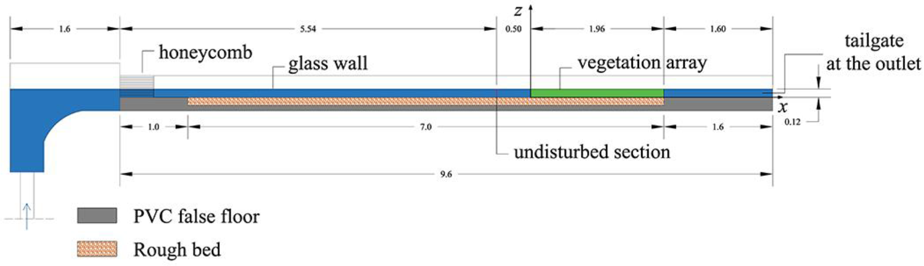
The experimental study was conducted in a 9.6-m long, 0.485-m wide and 0.5-m deep tilting flume at the Laboratorio “Grandi Modelli Idraulici” (GMI), Università della Calabria, Italy. In order to reduce the influence of the pump on the turbulence characteristics of the flow, a stilling tank, an uphill slipway and honeycombs (10 mm in diameter) were placed at the inlet of the channel. At the outlet, a tank equipped with a calibrated Thomson weir to measure the flow discharge Q and with a tailgate to regulate the water depth h of the flow were placed (Figure 1).
The experiments were carried out with a flow depth h ≈ 0.12 m, measured 50 cm upstream of the vegetation array (i.e., in undisturbed flow condition) by a point gauge with a decimal Vernier having an accuracy of ±0.1 mm and a flow discharge Q equal to 19.73 L/s (measured with a Thomson weir). The approaching cross-section average flow velocity U = Q/(Bh) was, hence, equal to 0.30 m s−1, where B was the flume width. The longitudinal bottom slope of the flume, S, was fixed at 1.5‰ using a hydraulic jack.
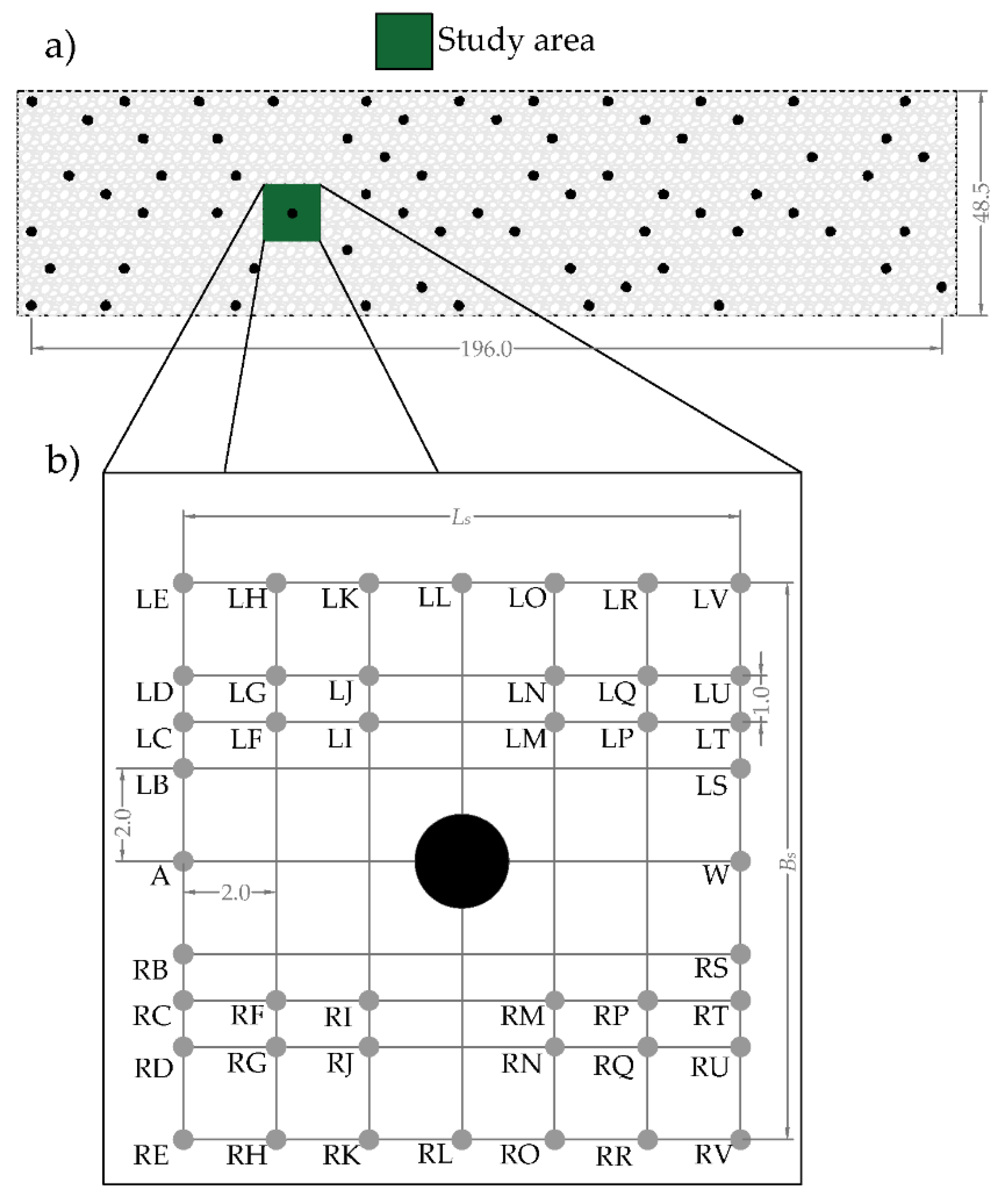
The rigid vegetation was simulated with vertical, wooden and circular cylinders. The cylinder height and diameter were hc = 0.40 m and d = 0.02 m, respectively. The stems were implanted into a 1.96-m long, 0.485-m wide and 0.015-m thick Plexiglas panel fixed to the channel bottom. A total of 68 cylinders were randomly arranged in the flume (Figure 2a). All the experiments were carried out in conditions of emergent vegetation. The frontal area per volume was a = nd = 1.4 m−1, where n = 71 m−2 was the number of cylinders per bed area, while the solid volume fraction occupied by the canopy els per bed area, while the solid volume fraction occupied by the canopy elements was ϕ = πad/4 = nπd24 = 0.02, which is consistent with typical laboratory studies with vegetation [17,26,27]. Following Nepf [28], this vegetation distribution can be classified as dense. Focus was given to the evolution of the turbulence characteristics in a study area selected around a single stem (Figure 2b).
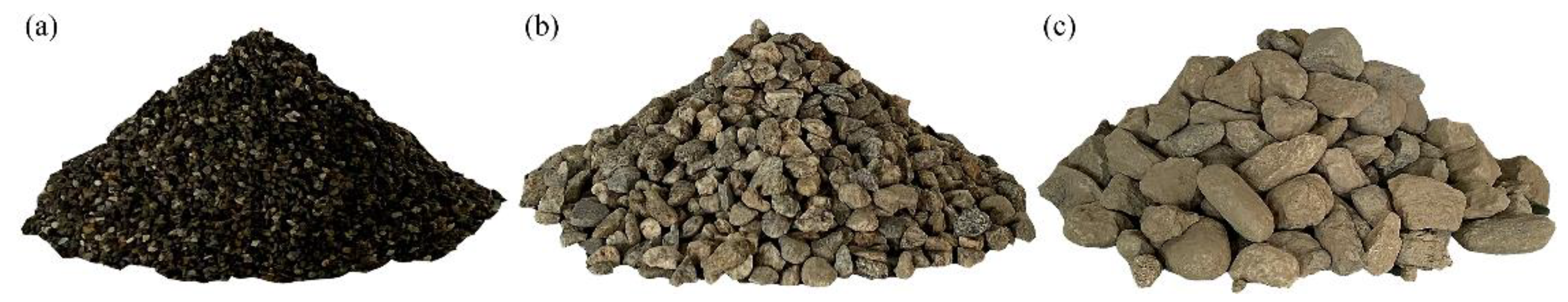
Three different types of bed roughness were simulated, employing very coarse sand (d50 = 1.53 mm), fine gravel (d50 = 6.49 mm) and coarse gravel (d50 = 17.98 mm), respectively (Figure 3). The grain size distributions were relatively uniform, i.e., as reported by Dey and Sarkar [29], with a geometric standard deviation σg = (d84/d16) 0.5 < 1.5, where d16 and d84 are the sediment sizes for which 16% and 84% by weight of sediment is finer, respectively. At the beginning of each run, the flume was filled in with the sediments, which were successively screeded to make the longitudinal bed slope equal to that of the flume bottom.
The experimental conditions used in this research do not reproduce a specific situation of a real river. Nevertheless, they could represent a new dataset that, for instance, may be used for the calibration of advanced numerical models. In fact, as is known, vegetation, bed roughness or man-made structures acting as an obstruction for the flow generate turbulence and affect the entire flow velocity distribution, modifying the turbulence behavior [30,31].
In Table 1, the hydraulic conditions of the experimental study are reported. Along with the aforementioned characteristics, in Table 1 the following quantities are listed: the shear velocity (u*), the critical velocity for the inception of sediment motion (Uc), the mean water temperature (T) measured with the Acoustic Doppler Velocimeter (ADV) integrated thermometer (having an accuracy of ±0.1 °C), the water kinematic viscosity (ν), computed as a function of the water temperature [32], the flow Froude number Fr [=U/(gh)0.5], the flow Reynolds number Re (=Uh/ν), the shear Reynolds number Re* (=u*ε/ν, where ε is the Nikuradse equivalent sand roughness, equal to about 2d50) and the Reynolds number of the vegetation stems Red (=Ud/ν). In accordance with Manes et al. [33] and Dey and Das [34], the shear velocity used to scale the flow statistics was determined as u*=(τ*/ρ)0.5, where τ* is the total stress acting at the roughness tops. This can be obtained by extending linearly the distribution of the turbulent shear stress captured 50 cm upstream of the vegetation pattern (i.e., in correspondence with the undisturbed flow condition) from the region above the roughness elements to their tops. Thus, the shear velocity was evaluated at the sediment crest level as , where u′ and w′ are the fluctuations of the temporal velocity signal in the streamwise and vertical directions, respectively, and the symbol indicates the time averaging operation. The critical velocity for the inception of sediment motion Uc was established 50 cm upstream of the vegetation array through the well-known Neill formula [35], as follows:
where g is the gravitational acceleration, Δ is the relative submerged grain density, is the grain density and is the fluid density. All the experiments were performed in clear-water condition (U < Uc), which was also verified from the direct observation of the flow.
An ADV profiler with down-looking probe, four beams (Nortek Vectrino) and an automatic movement system (the Traverse System by HR Wallingford Ltd., Oxfordshire UK) was used to capture the instantaneous velocity components (streamwise u, spanwise v and vertical w) with an accuracy of ±5% (assessed in previous works). The instrument sampling frequency was 100 Hz, and the duration of a single sampling was 300 s for a total number of samples of 30,000 which, as reported by [34,36,37], is adequate for determining accurate turbulence statistics. The sampling volume was a 1 mm long cylinder with a diameter of 6 mm. The ADV receivers pointed at 50 mm below their own transmitter. Hence, the measurements were not performed near the free surface flow zone (i.e., 50 mm below the free surface). The spatial coordinates of the Traverse System had an accuracy of ±0.1 mm. Prior to the analysis of the ADV data, it was necessary to proceed with the spike detection. Firstly, the ADV raw data were prefiltered, discarding the values with correlation (COR) lower than 70% and a signal-to-noise ratio (SNR) lower than 15 dB [34]; secondly, the contaminated velocity records were cleaned using the phase-space thresholding method and each spike was replaced with a cubic polynomial through 12 points on either side of itself [38]. The de-spiking method resulted in a rejection of less than 5% of the original velocity time series.
For all the runs, 44 vertical profiles were captured, as shown in Figure 2b. The vertical spatial resolutions were 3 mm for and 5 mm above, where z is the vertical axis starting from the maximum crest level in the study area.
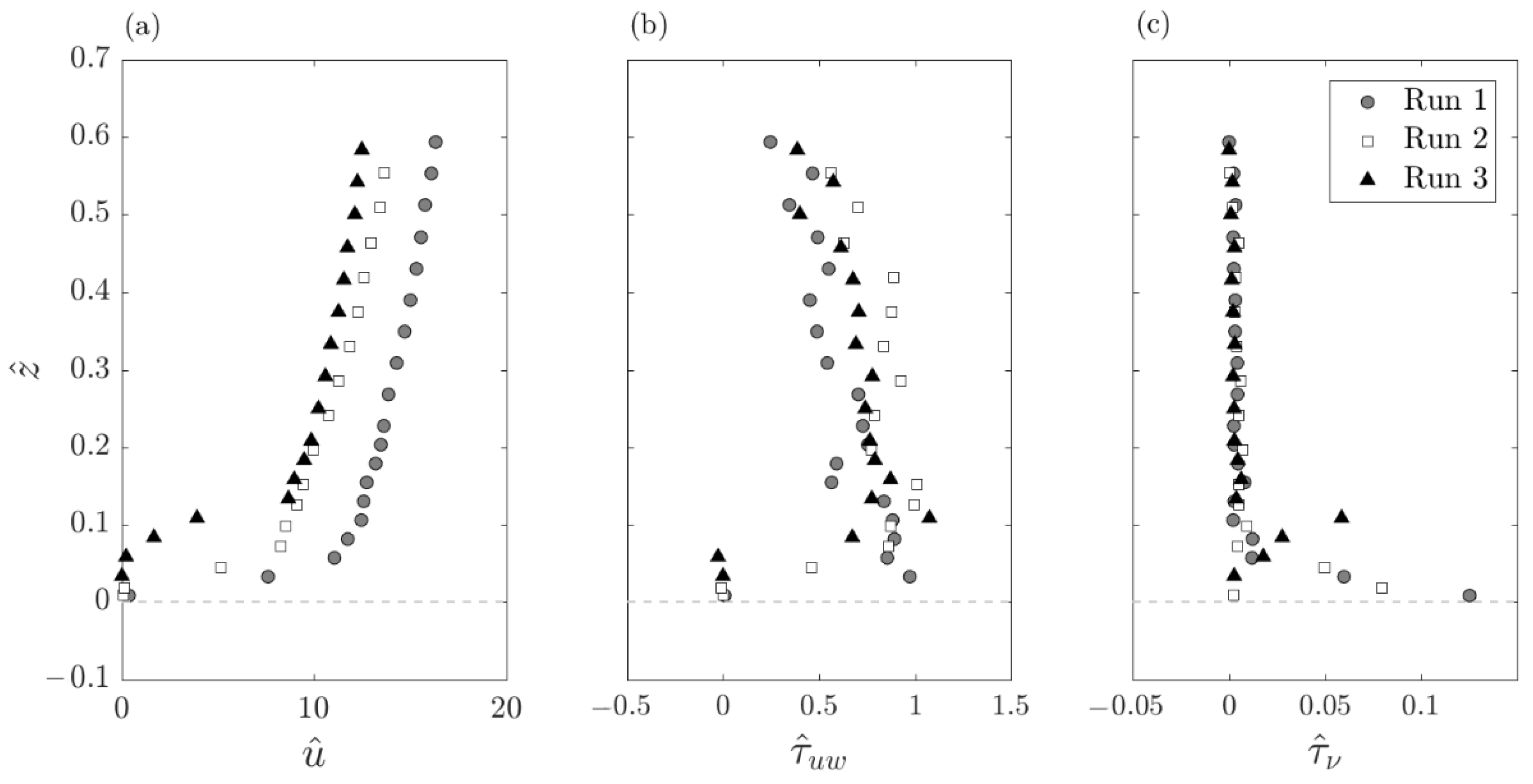
To describe the undisturbed flow 50 cm upstream of the vegetation array, the velocity vertical distribution was captured at the centerline of the laboratory flume during each run. In Figure 4a, the undisturbed profiles of the dimensionless time-averaged velocity in the streamwise direction (, where is the time-averaged velocity in the same direction) for the three experimental runs are reported. The vertical axis was made dimensionless by dividing the elevation z by the local water level that, for the undisturbed distributions, was equal to the flow depth h reported in Table 1. As the elevation z increases, the streamwise velocities u increase; instead, near the sediment grains, in the so-called roughness sublayer, they tend to zero owing to the bed roughness (this is typical in the open-channel flow condition) [39]. In particular, for Run 3, owing to higher roughness dimension, the streamwise velocity profile tended rapidly to zero starting from elevation z = 0.1h [40]. In addition, in the three runs shows different values at a fixed . This happens owing to the different bed roughness conditions that lead to an increase of the shear velocity as d50 increases and, consequently, to a decrease in . The distributions of the dimensionless turbulent shear stresses () and of the dimensionless viscous shear stresses [] along are represented in Figure 4b,c, respectively. In particular, above the roughness surface, the prevalence of the Reynolds shear stresses can be noted, while the viscous shear stresses are practically negligible as increases. The viscous shear stresses achieve their maximum values near the grain crests for each experimental run. Conversely, the turbulent shear stresses reach the peak above the crest level and then they reduce as the vertical distance increases.
3. Results and Discussion
3.1. Time-Averaged Flow
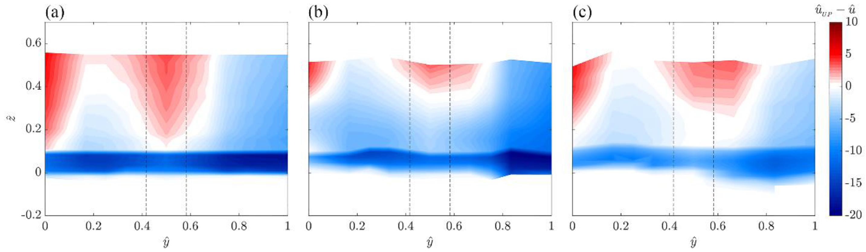
To investigate the time-averaged flow velocity field with respect to the approaching flow velocity in the spatial flow domain (i.e., in the upstream plane section identified with letters from LE to RE in the study area), Figure 5 shows the colormaps of the dimensionless time-averaged accelerated and decelerated flow fields upstream of the investigated stem in all the runs in the plane -. The abscissa, represented by , was made dimensionless by dividing y by the study area width (Bs = 12 cm). The time-averaged flow is accelerated if (blue values in the colormaps) and decelerated if (red values in the colormaps), where is the dimensionless time-averaged streamwise velocity.
A strong spanwise variation of can be noted with respect to the approaching flow profile. Specifically, in correspondence with the cylinder (), in all the runs the flow is decelerated. This probably occurs owing to the incidence of both the analyzed stem and another stem immediately upstream of the former (Figure 2a). An examination of the contours also reveals a decelerated flow zone on the left side of the cylinder (0) in all the experiments. This happens owing to the presence of another stem immediately upstream of the study area (Figure 2a). Instead, the flow fields are accelerated both on the right side of the analyzed cylinder and, to a lesser extent, on the left one. Moving toward the bed, it is evident that the flow velocity is also influenced by the bed roughness. As d50 decreases, this zone becomes strongly accelerated. Conversely, as d50 increases, in the near-bed layer, the flow field results to be influenced by the bed roughness and much more by the vegetation, with a minor acceleration intensity.
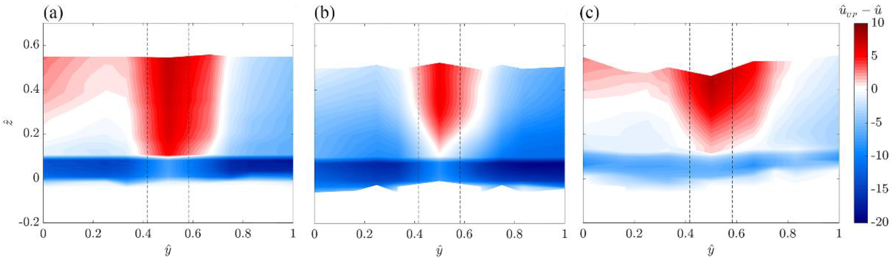
A similar behavior can be appreciated in the downstream flow domain in Figure 6 (i.e., in the downstream plane section identified with letters from LV to RV in the study area). In particular, immediately downstream of the cylinder (), the flow is decelerated in all the runs. Conversely, Run 2 shows an accelerated flow both on the right and on the left sides of the cylinder, while Run 1 and Run 3 show an accelerated flow mostly on the right side of the cylinder. A sensible difference is clear in the values of immediately upstream (vertical A; ) and downstream (vertical W; ) of the cylinder. Specifically, the time-averaged streamwise velocity is reduced by about 30% and 50% with respect to the time-averaged streamwise velocity of the undisturbed profile, , at the verticals A and W, respectively, in all the runs. It is possible to assure that a major deceleration is obtained beyond a cylinder. In fact, as observed in the downstream section at y = 0.5Bs (vertical W) with respect to the upstream section at y = 0.5Bs (vertical A), the velocity reduction is practically due to the vicinity of the studied stem (6 cm upstream). On the contrary, a minor deceleration is visible at vertical A, although it is between two cylinders (an upstream stem at 9 cm and a downstream stem at 6 cm).
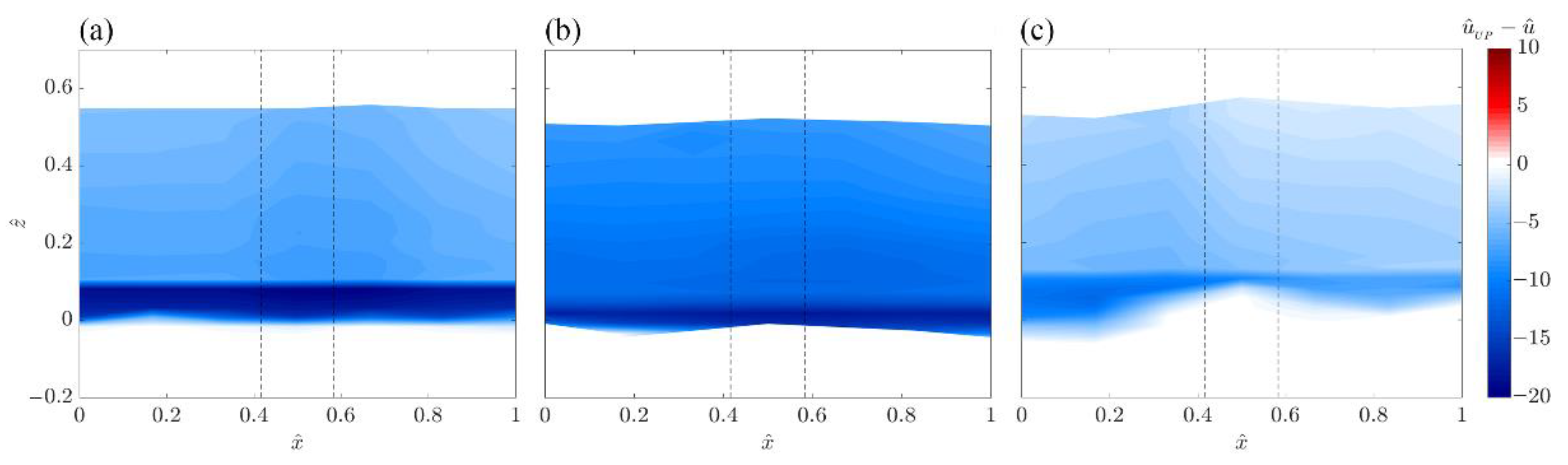
In order to investigate the longitudinal evolution of the flow field, the contours of the dimensionless time-averaged accelerated and decelerated flow field are analyzed. For the sake of simplicity, they are reported in Figure 7 only for the extreme right vertical plane identified with letters from RE to RV in the plane -. The abscissa was made dimensionless by dividing x by the study area width (Ls = 12 cm). In Figure 7, it is evident that the presence of vegetation has a very visible effect on the flow field: the flow is accelerated in all the runs with higher streamwise velocities than in the undisturbed flow profiles along the whole water depth. At each measurement location, the vegetation causes the velocity profile to maintain a constant value (for z > hl). Moving toward the bed (z < hl), the influence of vegetation decreases, and the flow field becomes more accelerated, owing to the presence of the bed.
3.2. TKE and Normal Stresses
The computation of the spatial distributions of the TKE is very significant in the assessment of the energetic process in open-channel flows. Since the time-averaged spatial fluctuations influence mechanical dispersion [41] and, in turn, this latter may be influenced by the vegetation stems and the bed roughness, the topic is of considerable interest. In fact, the presence of vegetation adds a further turbulence production in the wakes of the plant elements [42]. The TKE is defined as half the sum of the variances of the velocity components:
where v′ is the velocity fluctuation of the spanwise velocity v.
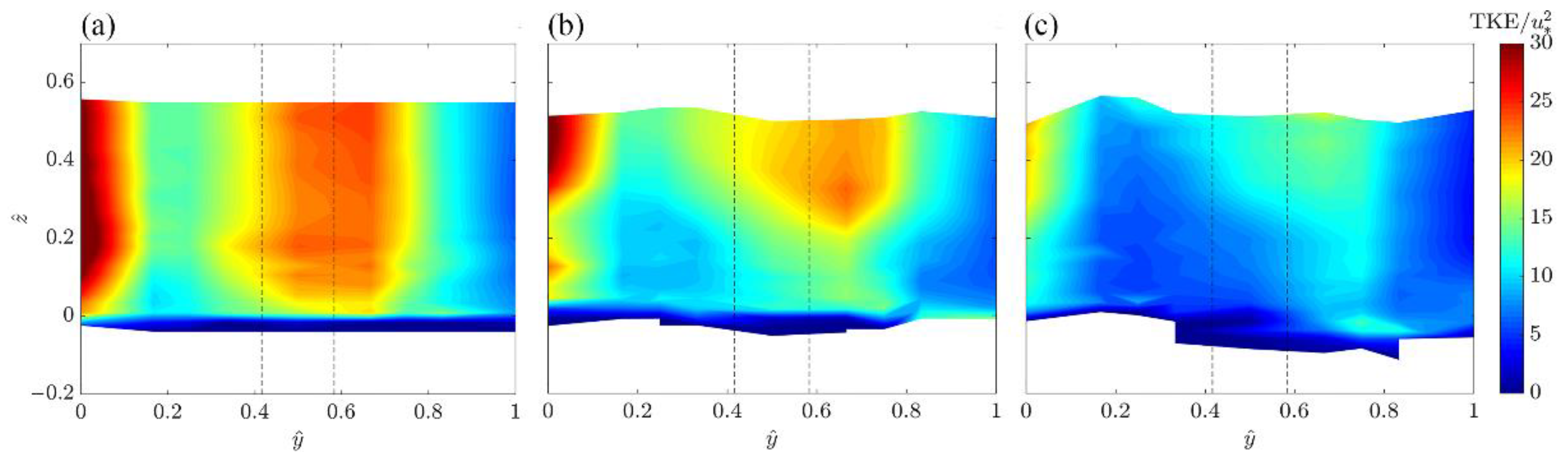
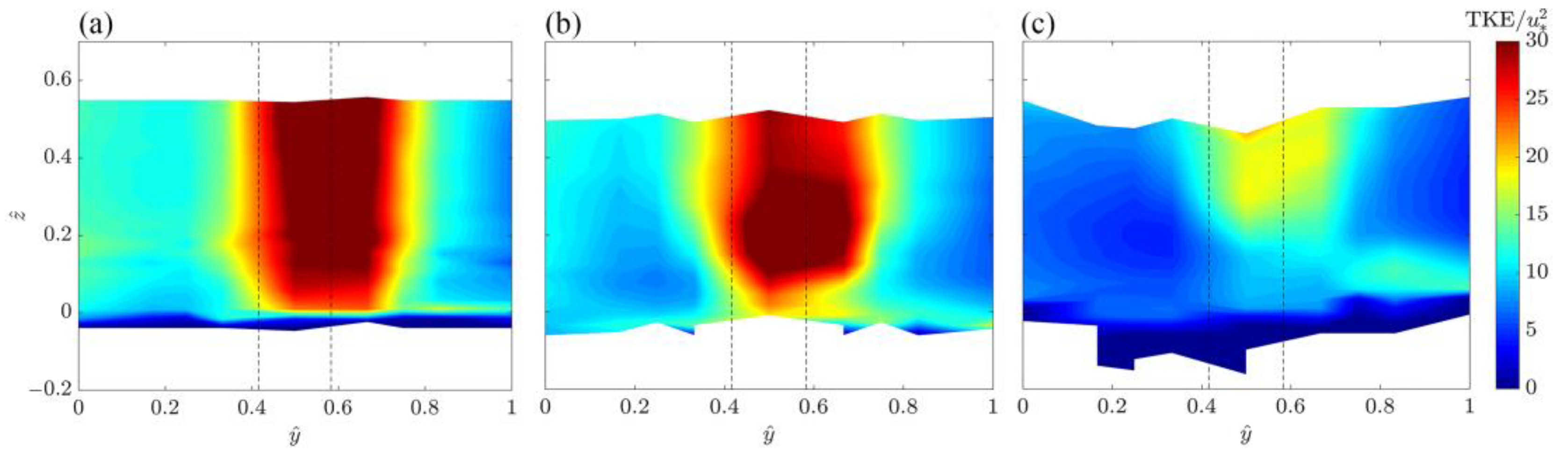
The colormaps of the dimensionless TKE (i.e., TKE divided by ) on the transversal upstream plane section (identified with the letters from LE to RE in the spanwise direction) are shown in Figure 8 for each experimental run. The highest values of the TKE are located in front of the cylinder and at the vertical LE (y = 0).
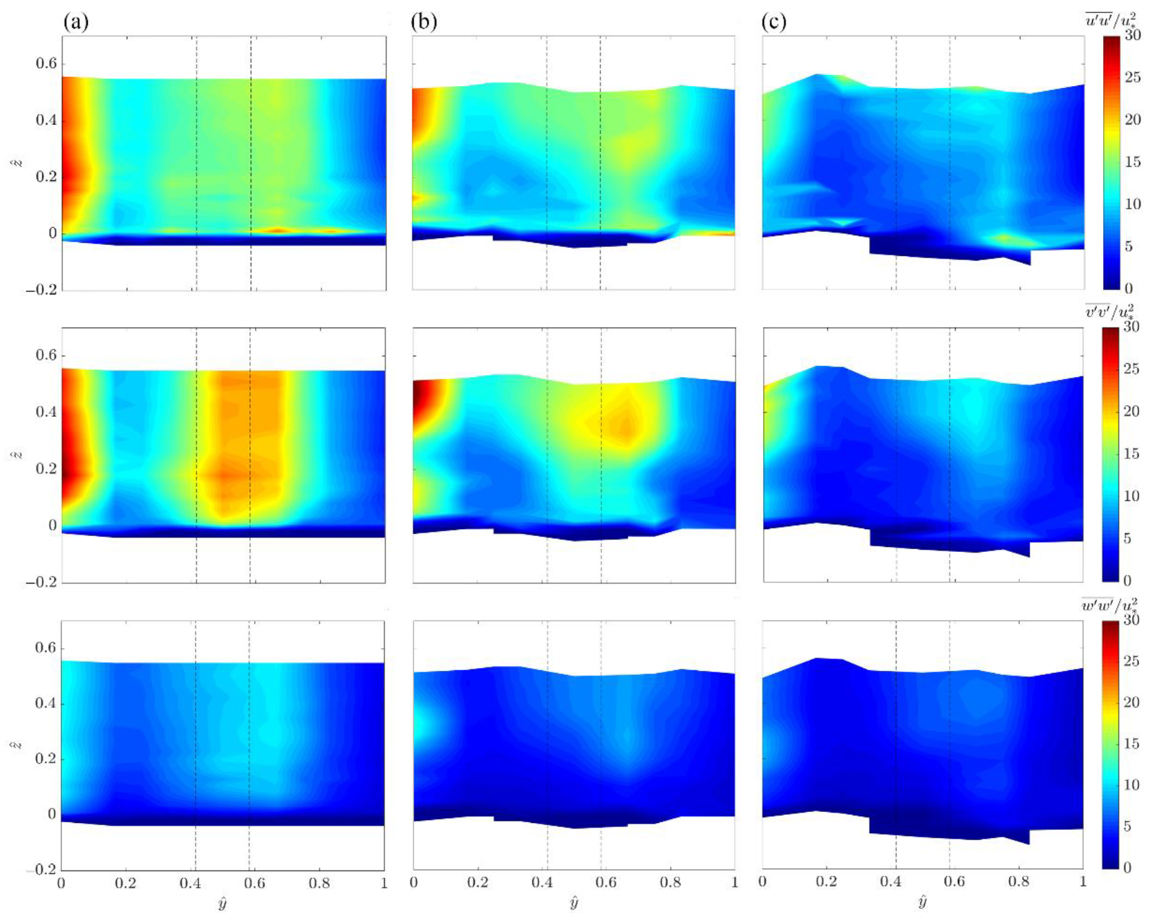
To analyze this behavior, in Figure 9 we consider, for all the runs, the dimensionless normal stresses in the streamwise, spanwise and vertical directions, , and , respectively, which are essentially the three addends in Equation (2). It is possible to observe that the high value on the left part of TKE contours (in Figure 8a) is practically ascribable to the streamwise and spanwise effects (Figure 9) owing to the presence upstream of the studied stem, both of an empty zone without vegetation, which influences , and of a wake vortex, that affects . In contrast, the high magnitude of the TKE immediately behind the vegetation element () is mostly due to the spanwise fluctuations, as a consequence of the circumvention of the obstacle.
Conversely, downstream of the studied vegetation element, the dimensionless TKE shows higher magnitudes immediately beyond the stem, whereas no high TKE value is detectable at y = 0 (Figure 10).
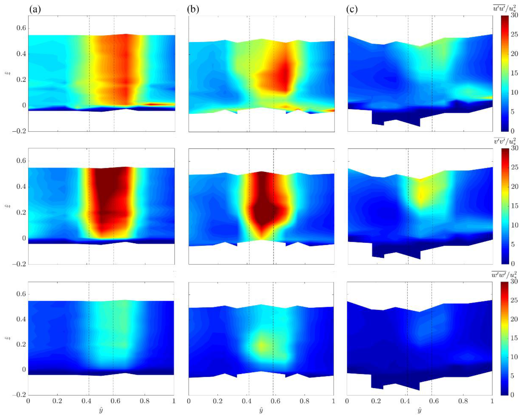
Analogously to the upstream flow field, from the normal shear stress distributions shown in Figure 11, it is possible to evaluate the contributions of the TKE patterns. Specifically, the higher kinetic energy values are influenced by both the streamwise, , and spanwise, normal stresses, which increase owing to the presence of the von Kármán wake vortex. This behavior, although with different magnitudes, is displayed in all the runs and, consequently, is clearly a vegetation effect. Furthermore, from a comparison between the TKE and the normal stress lateral distributions (Figure 8, Figure 10, and Figure 9, Figure 11, respectively), it is evident a predominant effect of the vegetation element in the downstream plane section and a contribution of the vertical normal stresses in the vertical W (downstream of the cylinder) greater than in the vertical A (upstream of the cylinder).
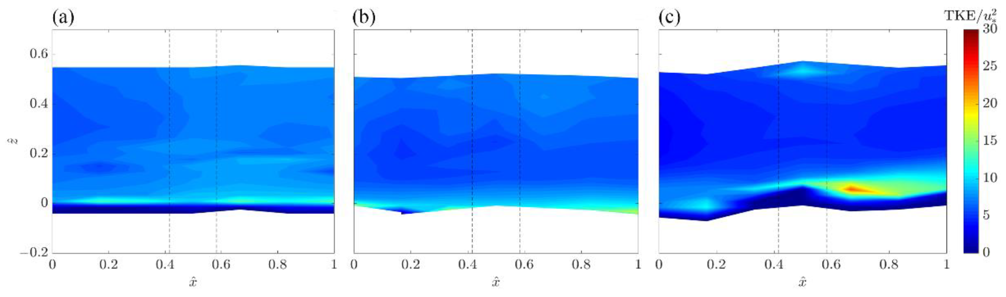
The distributions of the dimensionless TKE in the longitudinal extreme right vertical plane (identified with letters from RE to RV) are illustrated in Figure 12. High TKE magnitudes are observed in the near-bed flow zone, where the bed roughness surface causes higher fluctuations of the velocity components. However, the TKE reduces progressively moving upwards from z > 0, owing to the inhibition of u’, v’, and w’. The TKE contours are slightly spatially nonuniform for all the experiments. This is probably due to the random vegetation array and the spatial irregular bed sediment.
3.3. Energy Spectra
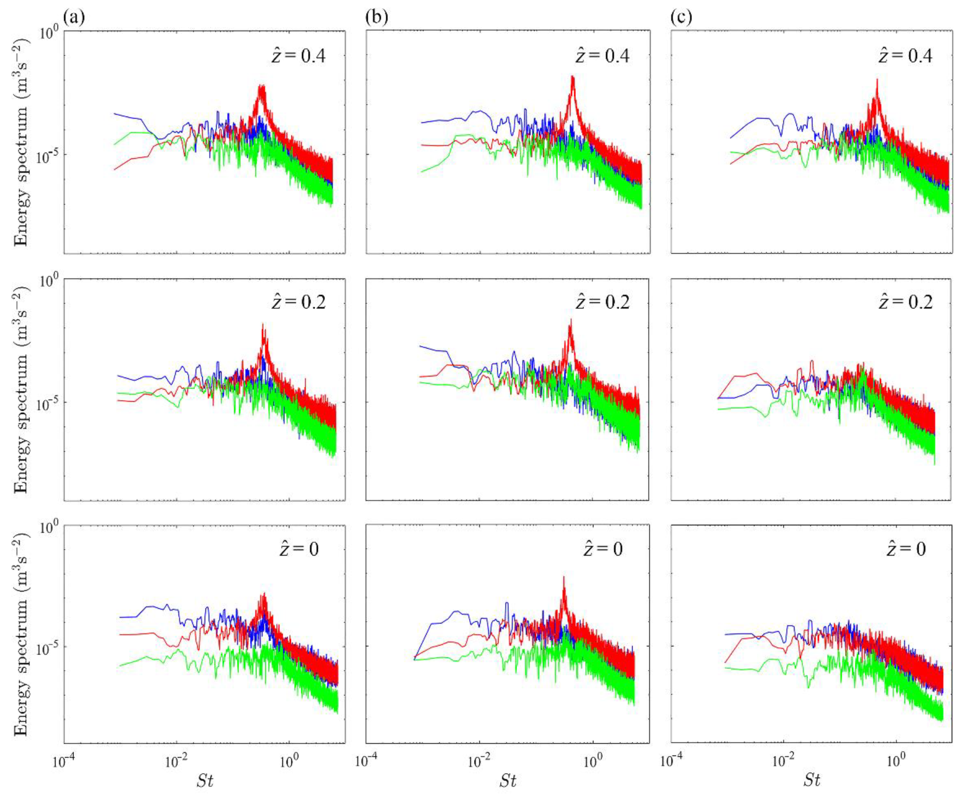
In order to further analyze the turbulent characteristics, the measured velocity data were explored through the energy spectra of the velocity fluctuations. In particular, the energy spectra are shown in Figure 13 for the vertical W, i.e., immediately downstream of the studied cylinder for all the runs and three different elevations (z = 0, z = 0.2 h and z = 0.4 h), as a function of the Strouhal number of the cylinder (St = fd/, where f is the frequency with a resolution equal to Fs/N, and N is the number of samples equal to 30,000 for an acquisition time of 300 s). The energy spectra were determined by employing the discrete fast Fourier transform of the autocorrelation function.
From a comparison of the spectra, the spanwise velocity revealed the presence of large-scale coherent structures, evident as a peak located in the energy-containing range of the energy spectra (Figure 13). Specifically, these peaks are present in all the runs, with the exception of two spectra of Run 3, where it is evident that the peak recedes as z decreases. This may be due to a roughness effect, which in Run 3 is explicated with a medium sediment diameter equal to 17.98 mm, i.e., comparable with the stem diameter, equal to 20 mm. Moreover, the peaks were observed at the same Strouhal number in the u’v’ cross-spectra (not shown here for the sake of brevity), demonstrating that the identified coherent structures were responsible across the vegetation for the lateral momentum transport [5].
4. Conclusions
In the present work, an experimental study was carried out to investigate the impact of different uniform bed roughness on the flow characteristics through randomly arranged emergent rigid vegetation. In particular, focus was given to the evolution of the turbulence characteristics in a study area selected around a single stem. The principal results are summarized below.
In the sections, respectively, upstream and downstream of the generic stem, the dimensionless time-averaged accelerated and decelerated flow field is deeply affected by the vegetation and, to a lesser extent, by the bed roughness. In particular, in the flow field downstream of the studied cylinder it is possible to point out these zones: a decelerated one, in correspondence to the stem (), another decelerated zone, on the left side of the stem (0 , only for Runs 1 and 3) and an accelerated one elsewhere.
From a comparison perspective, it is possible to evaluate a velocity reduction of about 50% in the downstream plane immediately behind the analyzed stem. Conversely, downstream of the cylinder, on the left side (0), the decelerated zones fade about 30%. This is clearly attributable to the random distribution of the vegetation pattern. Instead, in the longitudinal plane the flow is decelerated in all the runs with higher streamwise velocities than in the undisturbed flow profiles along the whole water depth.
The analysis of the TKE distribution clearly shows the effects of the vegetation, with high magnitudes immediately upstream and downstream of the investigated stem. This indicates that the velocity oscillations get excited by the cylinders, producing an increased turbulence intensity in the proximity of the stem. Moving toward the free zone (i.e., without vegetation), this influence vanishes, causing a decrease in the TKE value. In addition, the behavior observed in TKE colormaps was examined by comparing the streamwise, spanwise and vertical normal stress contours. The results revealed a strong influence of the u’ and v’ fluctuations on the energy distribution and highlighted the influence of the so-called von Kármán vortices. In addition, from the analysis of the TKE distributions, an effect of the cylinder greater in the downstream plane section than in the upstream one is manifested, with an increased mean value of 25% at the abscissa y = 0.5 Bs. The longitudinal TKE distribution revealed high values in the near-bed flow zone. This suggests that the velocity oscillations get excited by the rough bed, producing an increase of the turbulence level in the vicinity of the sediments. Mowing toward the free surface this effect disappears, inducing a decrease in the TKE.
The evaluation of the energy spectra of the velocity fluctuations showed a clear influence of both vegetation and roughness. In particular, the spanwise velocity component revealed energetic peaks that indicate the presence of large-scale coherent structures due to the von Kármán wake vortex along the flow depth in the case of lower roughness (Run 1 and 2) and only in the upper part of the water depth in the case of higher roughness (Run 3). In fact, it is interesting to point out that, when the median sediment diameter is comparable with the stem diameter (i.e., Run 3) going towards the bed, the energetic peak is lowered. This involves a consideration of the nature of coherent structures of turbulence, which are significantly influenced by the characteristic scales of the flow conditions, such as vegetation diameter, water depth and roughness size.
Further study is necessary to describe more deeply the turbulence structures in the presence of both vegetation and sediments. In fact, the results referring to a single generic cylinder are representative only for such a case and cannot be generalized, owing to the lack of further data relating to different vegetation elements. For this purpose, in future works we intend to perform other laboratory experiments, intensifying the measurements and adopting advanced techniques, such as the Particle Image Velocimetry (PIV), in order to better characterize the two-dimensional (2D) turbulence structures.
Author Contributions
Conceptualization, F.C., N.P., A.P.F., R.G.; methodology, F.C., N.P., P.G., R.G.; formal analysis, F.C., N.P.; data curation, F.C.; writing—original draft preparation, F.C.; writing—review and editing, F.C., N.P., A.P.F., P.G., R.G.; supervision, R.G.; funding acquisition, R.G. All authors have read and agreed to the published version of the manuscript.
Funding
This research was funded by the “SILA-Sistema Integrato di Laboratori per l’Ambiente-An Integrated System of Laboratories for the Environment” PONa3_00341.
Data Availability Statement
Publicly available datasets were analyzed in this study. This data can be found here: http://www.ingegneriacivile.unical.it/lgmi/turbulent-flow-through-random-vegetation-on-a-rough-bed/, accessed on 14 September 2021.
Acknowledgments
The authors would like to thank Erik Calabrese Violetta for his valuable work during the performance of the experimental runs.
Conflicts of Interest
The authors declare no conflict of interest.
References
- White, B.L.; Nepf, H.M. A vortex-based model of velocity and shear stress in a partially vegetated shallow channel. Water Resour. Res. 2008, 44, 1–15. [Google Scholar] [CrossRef]
- Meftah, M.B.; De Serio, F.; Mossa, M. Hydrodynamic behavior in the outer shear layer of partly obstructed open channels. Phys. Fluids 2014, 26, 065102. [Google Scholar] [CrossRef]
- Caroppi, G.; Gualtieri, P.; Fontana, N.; Giugni, M. Vegetated channel flows: Turbulence anisotropy at flow–rigid canopy interface. Geosciences 2018, 8, 259. [Google Scholar] [CrossRef] [Green Version]
- Rowiński, P.M.; Västilä, K.; Aberle, J.; Järvelä, J.; Kalinowska, M.B. How vegetation can aid in coping with river management challenges: A brief review. Ecohydrol. Hydrobiol. 2018, 18, 345–354. [Google Scholar] [CrossRef] [Green Version]
- Caroppi, G.; Västilä, K.; Järvelä, J.; Rowiński, P.M.; Giugni, M. Turbulence at water-vegetation interface in open channel flow: Experiments with natural-like plants. Adv. Water Resour. 2019, 127, 180–191. [Google Scholar] [CrossRef]
- Kemp, J.; Harper, D.; Crosa, G. The habitat-scale ecohydraulics of rivers. Ecol. Eng. 2000, 16, 17–29. [Google Scholar] [CrossRef]
- Nepf, H.M. Hydrodynamics of vegetated channels. J. Hydraul. Res. 2012, 50, 262–279. [Google Scholar] [CrossRef] [Green Version]
- Västilä, K.; Järvelä, J. Modeling the flow resistance of woody vegetation using physically based properties of the foliage and stem. Water Resour. Res. 2014, 50, 229–245. [Google Scholar] [CrossRef]
- Nepf, H.M.; Vivoni, E.R. Flow structure in depth-limited, vegetated flow. J. Geophys. Res. Oceans 2000, 105, 28547–28557. [Google Scholar] [CrossRef]
- Järvelä, J. Effect of submerged flexible vegetation on flow structure and resistance. J. Hydrol. 2005, 307, 233–241. [Google Scholar] [CrossRef]
- Li, C.W.; Xie, J. FNumerical modeling of free surface flow over submerged and highly flexible vegetation. Adv. Water Resour. 2011, 34, 468–477. [Google Scholar] [CrossRef]
- Maji, S.; Hanmaiahgari, P.R.; Balachandar, R.; Pu, J.H.; Ricardo, A.M.; Ferreira, R.M. A Review on Hydrodynamics of Free Surface Flows in Emergent Vegetated Channels. Water 2020, 12, 1218. [Google Scholar] [CrossRef]
- Ricardo, A.M.; Franca, M.J.; Ferreira, R.M. Turbulent flows within random arrays of rigid and emergent cylinders with varying distribution. J. Hydraul. Eng. 2016, 142, 04016022. [Google Scholar] [CrossRef]
- Nezu, I.; Sanjou, M. Turburence structure and coherent motion in vegetated canopy open-channel flows. J. Hydro-Environ. Res. 2008, 2, 62–90. [Google Scholar] [CrossRef]
- Yang, W.; Choi, S.U. A two-layer approach for depth-limited open-channel flows with submerged vegetation. J. Hydraul. Res. 2010, 48, 466–475. [Google Scholar] [CrossRef]
- Shimizu, Y.; Tsujimoto, T. Numerical analysis of turbulent open-channel flow over a vegetation layer using a k-ε turbulence model. J. Hydrosci. Hydraul. Eng. 1994, 11, 57–67. [Google Scholar]
- Nepf, H. Drag, turbulence, and diffusion in flow through emergent vegetation. Water Resour. Res. 1999, 35, 479–489. [Google Scholar] [CrossRef]
- Righetti, M.; Armanini, A. Flow resistance in open channel flows with sparsely distributed bushes. J. Hydrol. 2002, 269, 55–64. [Google Scholar] [CrossRef]
- Choi, S.U.; Kang, H. Numerical investigations of mean flow and turbulence structures of partly-vegetated open-channel flows using the Reynolds stress model. J. Hydraul. Res. 2006, 44, 203–217. [Google Scholar] [CrossRef]
- Poggi, D.; Krug, C.; Katul, G.G. Hydraulic resistance of submerged rigid vegetation derived from first-order closure models. Water Resour. Res. 2009, 45, W10442. [Google Scholar] [CrossRef]
- Gualtieri, P.; De Felice, S.; Pasquino, V.; Doria, G. Use of conventional flow resistance equations and a model for the Nikuradse roughness in vegetated flows at high submergence. J. Hydrol. Hydromech. 2018, 66, 107–120. [Google Scholar] [CrossRef] [Green Version]
- Liu, D.; Diplas, P.; Fairbanks, J.D.; Hodges, C.C. An experimental study of flow through rigid vegetation. J. Geophys. Res. Earth Surf. 2008, 113, F04015. [Google Scholar] [CrossRef]
- De Serio, F.; Ben Meftah, M.; Mossa, M.; Termini, D. Experimental investigation on dispersion mechanisms in rigid and flexible vegetated beds. Adv. Water Resour. 2018, 120, 98–113. [Google Scholar] [CrossRef]
- Penna, N.; Coscarella, F.; D’Ippolito, A.; Gaudio, R. Bed roughness effects on the turbulence characteristics of flows through emergent rigid vegetation. Water 2020, 12, 2401. [Google Scholar] [CrossRef]
- Penna, N.; Coscarella, F.; D’Ippolito, A.; Gaudio, R. Anisotropy in the free stream region of turbulent flows through emergent rigid vegetation on rough bed. Water 2020, 12, 2464. [Google Scholar] [CrossRef]
- Petryk, S. Drag on Cylinders in Open Channel Flow. Ph.D. Thesis, Colorado State University, Fort Collins, CO, USA, 1969. [Google Scholar]
- Stone, B.M.; Shen, H.T. Hydraulic resistance of flow in channels with cylindrical roughness. J. Hydraul. Eng. 2002, 128, 500–506. [Google Scholar] [CrossRef]
- Nepf, H.M. Flow and transport in regions with aquatic vegetation. Annu. Rev. Fluid Mech. 2012, 44, 123–142. [Google Scholar] [CrossRef] [Green Version]
- Dey, S.; Sarkar, A. Scour downstream of an apron due to submerged horizontal jets. J. Hydraul. Eng. 2006, 132, 246–257. [Google Scholar] [CrossRef]
- Penna, N.; Coscarella, F.; Gaudio, R. Turbulent Flow Field around Horizontal Cylinders with Scour Hole. Water 2020, 12, 143. [Google Scholar] [CrossRef] [Green Version]
- Pu, J.H.; Hussain, A.; Guo, Y.K.; Vardakastanis, N.; Hanmaiahgari, P.R.; Lam, D. Submerged flexible vegetation impact on open channel flow velocity distribution: An analytical modelling study on drag and friction. Water Sci. Eng. 2019, 12, 121–128. [Google Scholar] [CrossRef]
- Julien, P.Y. Erosion and Sedimentation; Cambridge University Press: Cambridge, UK, 1998. [Google Scholar]
- Manes, C.; Pokrajac, D.; McEwan, I. Double-averaged open-channel flows with small relative submergence. J. Hydraul. Eng. 2007, 133, 896–904. [Google Scholar] [CrossRef]
- Dey, S.; Das, R. Gravel-bed hydrodynamics: Double-averaging approach. J. Hydraul. Eng. 2012, 138, 707–725. [Google Scholar] [CrossRef]
- Neill, C.R. Mean-velocity criterion for scour of coarse uniform bed material. In Proceedings of the International Association of Hydraulic Research 12th Congress, Fort Collins, CO, USA, 11–14 September 1967; pp. 46–54. [Google Scholar]
- Strom, K.B.; Papanicolaou, A.N. ADV measurements around a cluster microform in a shallow mountain stream. J. Hydraul. Eng. 2007, 133, 1379–1389. [Google Scholar] [CrossRef]
- Afzalimehr, H.; Moghbel, R.; Gallichand, J.; Jueyi, S.U.I. Investigation of turbulence characteristics in channel with dense vegetation. Int. J. Sediment Res. 2011, 26, 269–282. [Google Scholar] [CrossRef]
- Goring, D.G.; Nikora, V.I. Despiking acoustic Doppler velocimeter data. J. Hydraul. Eng. 2002, 128, 117–126. [Google Scholar] [CrossRef] [Green Version]
- Dey, S. Fluvial Hydrodynamics; Springer: Heidelberg, Germany, 2014. [Google Scholar]
- Dey, S.; Sarkar, S.; Ballio, F. Double-averaging turbulence characteristics in seeping rough-bed streams. J. Geophys. Res. Earth Surf. 2011, 116. [Google Scholar] [CrossRef]
- Tanino, Y.; Nepf, H. Lateral dispersion in random cylinder arrays at high Reynolds number. J. Fluid Mech. 2008, 600, 339–371. [Google Scholar] [CrossRef] [Green Version]
- Defina, A.; Bixio, A.C. Mean flow and turbulence in vegetated open channel flow. Water Resour. Res. 2005, 41, W07006. [Google Scholar] [CrossRef] [Green Version]
Figure 1.
Schematic of the experimental facility (dimensions are expressed in meters).

Figure 2.
(a) Sketch of the cylinder array in the laboratory flume (dimensions are in cm); (b) the measurement verticals within the study area. Here, Bs and Ls are the width and length of the study area, respectively.
Figure 2.
(a) Sketch of the cylinder array in the laboratory flume (dimensions are in cm); (b) the measurement verticals within the study area. Here, Bs and Ls are the width and length of the study area, respectively.

Figure 3.
Sediments used in the experimental runs: (a) d50 = 1.53 mm; (b) d50 = 6.49 mm; (c) d50 = 17.98 mm.
Figure 3.
Sediments used in the experimental runs: (a) d50 = 1.53 mm; (b) d50 = 6.49 mm; (c) d50 = 17.98 mm.

Figure 4.
Vertical profiles of (a) dimensionless time-averaged velocity, (b) dimensionless Reynolds shear stress and (c) dimensionless viscous shear stress for the undisturbed flow condition (50 cm upstream to the vegetation array) in Run 1, Run 2 and Run 3.
Figure 4.
Vertical profiles of (a) dimensionless time-averaged velocity, (b) dimensionless Reynolds shear stress and (c) dimensionless viscous shear stress for the undisturbed flow condition (50 cm upstream to the vegetation array) in Run 1, Run 2 and Run 3.

Figure 5.
Contours of the dimensionless time-averaged accelerated and decelerated flow field in the upstream plane section (from LE to RE) for (a) Run 1, (b) Run 2 and (c) Run 3. The black dashed lines show the cylinder position.
Figure 5.
Contours of the dimensionless time-averaged accelerated and decelerated flow field in the upstream plane section (from LE to RE) for (a) Run 1, (b) Run 2 and (c) Run 3. The black dashed lines show the cylinder position.

Figure 6.
Contours of the dimensionless time-averaged accelerated and decelerated flow field in the downstream plane section (from LV to RV) for (a) Run 1, (b) Run 2 and (c) Run 3. The black dashed lines show the cylinder position.
Figure 6.
Contours of the dimensionless time-averaged accelerated and decelerated flow field in the downstream plane section (from LV to RV) for (a) Run 1, (b) Run 2 and (c) Run 3. The black dashed lines show the cylinder position.

Figure 7.
Contours of the dimensionless time-averaged accelerated and decelerated flow field in the longitudinal plane section (from RE to RV) for (a) Run 1, (b) Run 2 and (c) Run 3. The black dashed lines show the cylinder position.
Figure 7.
Contours of the dimensionless time-averaged accelerated and decelerated flow field in the longitudinal plane section (from RE to RV) for (a) Run 1, (b) Run 2 and (c) Run 3. The black dashed lines show the cylinder position.

Figure 8.
Contours of the dimensionless TKE in the upstream plane section (from LE to RE) for (a) Run 1, (b) Run 2 and (c) Run 3. The black dashed lines show the cylinder position.
Figure 8.
Contours of the dimensionless TKE in the upstream plane section (from LE to RE) for (a) Run 1, (b) Run 2 and (c) Run 3. The black dashed lines show the cylinder position.

Figure 9.
Contours of the dimensionless normal stresses (a) , (b) and (c) in the upstream plane section (from LE to RE) for (a) Run 1, (b) Run 2 and (c) Run 3. The black dashed lines show the cylinder position.
Figure 9.
Contours of the dimensionless normal stresses (a) , (b) and (c) in the upstream plane section (from LE to RE) for (a) Run 1, (b) Run 2 and (c) Run 3. The black dashed lines show the cylinder position.

Figure 10.
Contours of the dimensionless TKE in the downstream plane section (from LV to RV) for (a) Run 1, (b) Run 2 and (c) Run 3. The black dashed lines show the cylinder position.
Figure 10.
Contours of the dimensionless TKE in the downstream plane section (from LV to RV) for (a) Run 1, (b) Run 2 and (c) Run 3. The black dashed lines show the cylinder position.

Figure 11.
Contours of the dimensionless normal stresses (a) , (b) and (c) in the downstream plane section (from LV to RV) for (a) Run 1, (b) Run 2 and (c) Run 3. The black dashed lines show the cylinder position.
Figure 11.
Contours of the dimensionless normal stresses (a) , (b) and (c) in the downstream plane section (from LV to RV) for (a) Run 1, (b) Run 2 and (c) Run 3. The black dashed lines show the cylinder position.

Figure 12.
Contours of the dimensionless TKE in the longitudinal plane section (from RE to RV) for (a) Run 1, (b) Run 2 and (c) Run 3. The black dashed lines show the cylinder position.
Figure 12.
Contours of the dimensionless TKE in the longitudinal plane section (from RE to RV) for (a) Run 1, (b) Run 2 and (c) Run 3. The black dashed lines show the cylinder position.

Figure 13.
Energy spectra for (a) Run 1, (b) Run 2 and (c) Run 3 of streamwise (blue lines), spanwise (red lines), and vertical (green lines) velocity fluctuations at three different levels of the vertical W.
Figure 13.
Energy spectra for (a) Run 1, (b) Run 2 and (c) Run 3 of streamwise (blue lines), spanwise (red lines), and vertical (green lines) velocity fluctuations at three different levels of the vertical W.


Table 1.
Hydraulic conditions of the experimental study for the approaching flow.
| Parameter (Units) | Run 1 | Run 2 | Run 3 |
|---|---|---|---|
| d50 (mm) | 1.53 | 6.49 | 17.98 |
| h (m) | 0.12 | 0.12 | 0.12 |
| Q (l/s) | 19.73 | 19.73 | 19.73 |
| U (m/s) | 0.34 | 0.34 | 0.34 |
| u* (m/s) | 0.021 | 0.022 | 0.028 |
| Uc (m/s) | 0.39 | 0.69 | 1.04 |
| S (‰) | 1.50 | 1.50 | 1.50 |
| T (°C) | 16.67 | 18.06 | 18.70 |
| ν (m 2/s) | 1.09 × 10⁻⁶ | 1.05 × 10⁻⁶ | 1.03 × 10⁻⁶ |
| Fr | 0.31 | 0.31 | 0.31 |
| Re | 37,431 | 38,857 | 39,612 |
| Re* | 59 | 272 | 978 |
| Red | 6239 | 6192 | 6602 |
Publisher’s Note: MDPI stays neutral with regard to jurisdictional claims in published maps and institutional affiliations. |
© 2021 by the authors. Licensee MDPI, Basel, Switzerland. This article is an open access article distributed under the terms and conditions of the Creative Commons Attribution (CC BY) license (https://creativecommons.org/licenses/by/4.0/).
Share and Cite
MDPI and ACS Style
Coscarella, F.; Penna, N.; Ferrante, A.P.; Gualtieri, P.; Gaudio, R. Turbulent Flow through Random Vegetation on a Rough Bed. Water 2021, 13, 2564. https://doi.org/10.3390/w13182564
AMA Style
Coscarella F, Penna N, Ferrante AP, Gualtieri P, Gaudio R. Turbulent Flow through Random Vegetation on a Rough Bed. Water. 2021; 13(18):2564. https://doi.org/10.3390/w13182564
Chicago/Turabian StyleCoscarella, Francesco, Nadia Penna, Aldo Pedro Ferrante, Paola Gualtieri, and Roberto Gaudio. 2021. "Turbulent Flow through Random Vegetation on a Rough Bed" Water 13, no. 18: 2564. https://doi.org/10.3390/w13182564
Note that from the first issue of 2016, this journal uses article numbers instead of page numbers. See further details here.