Corrections of Precipitation Particle Size Distribution Measured by a Parsivel OTT² Disdrometer under Windy Conditions in the Antisana Massif, Ecuador

Abstract

Monitoring precipitation in mountainous areas using traditional tipping-bucket rain gauges (TPB) has become challenging in sites with strong variations of air temperature and wind speed (Ws). The drop size distributions (DSD), amount, and precipitation-type of a Parsivel OTT² disdrometer installed at 4730 m above sea level (close to the 0 °C isotherm) in the glacier foreland of the Antisana volcano in Ecuador are used to analyze the precipitation type. To correct the DSDs, we removed spurious particles and shifted fall velocities such that the mean value matches with the fall velocity–diameter relationship of rain, snow, graupel, and hail. Solid (SP) and liquid precipitation (LP) were identified through −1 and 3 °C thresholds and then grouped into low, medium, and high Ws categories by k-means approach. Changes in DSDs were tracked using concentration spectra and particle’s contribution by diameter and fall velocity. Thus, variations of concentration/dispersion and removed hydrometeors were linked with Ws changes. Corrected precipitation, assuming constant density (1 g cm⁻³), gives reliable results for LP with respect to measurements at TPB and overestimates SP measured in disdrometer. Therefore, corrected precipitation varying density models achieved fewer differences. These results are the first insight toward the understating of precipitation microphysics in a high-altitude site of the tropical Andes.

1. Introduction

An adequate measurement of precipitation reaching the ground is essential to picture its spatial and temporal variability accurately. This allows to reduce the uncertainty in hydrological simulations [1], to improve forecasting and early warning tools [2,3], and appropriate water management [4,5]. However, this becomes challenging in mountainous regions, where the observations of solid and liquid precipitations are strongly affected by wind [6].

A rain gauge acts as an obstacle that disturbs the incoming airflow originating turbulence and eddies around, resulting in deflected trajectories of some hydrometeors away from the funnel region and missing the gauge orifice [7,8]. The reduction of particle flow over the gauge (under-catch) due to wind effect depends on wind speed, precipitation type, rainfall intensity, and the aerodynamic design of the rain-gauge [9,10,11,12]. It is especially true for solid precipitation collected by unshielded gauges, where analyzing the measured precipitation characteristics becomes more complex [13,14,15]. Thus, from the literature, it is concluded that traditional rain gauges are little reliable for precipitation collection under windy conditions.

To analyze the impact of the wind speed on the measurements of solid and liquid precipitation, a Parsivel OTT² disdrometer was installed near the glacier of Antisana volcano in Ecuador at 4730 m above sea level (m asl) (Figure 1). Disdrometers are a practical alternative due to the low maintenance required, including for harsh conditions. Among the advantages of this device, are: (1) it avoids contact with particles due to its optical method of measurement [16,17]; (2) due to its sensitivity, it can measure events with precipitation less than 0.1 mm h⁻¹ with a high temporal resolution [18,19]; (3) it offers the possibility of detecting the type of precipitation [16,20]. These characteristics make the gathered data a valuable information source about the fine-scale structure of precipitation which is currently limited to only the páramo zone (high altitude wet grassland) around 3780 m asl [21].

However, disdrometers are prone to record erroneous fall velocity raindrops mostly due to particles falling through the edges of the sample area [23], in addition to strong winds leading to misclassification of particles [24]. Several studies show that the Parsivel OTT² tends to overestimate the fall velocity of small raindrops [17,25] and underestimate the fall speed of small snowflakes [26,27] and large raindrops [20,28,29]. To the authors’ best knowledge, the evaluation of the impact of corrections for different fall velocities on solid and liquid precipitation is missing to date.

Therefore, the measured particle size distributions (DSDs) need to be corrected to compute precipitation adequately. The methods developed to correct DSD are based on the removal of hydrometeors outside of a threshold range of the empirical fall velocity–diameter relationship [17,20], while others establish a threshold to remove particles out of a diameter range [30]. However, they seem inappropriate for the study site since they were conceived for only rainfall (liquid precipitation) and high latitudes. Instead, the method proposed by Raupach and Berne [25] has been recommended and employed by various studies (e.g., [29,31,32,33]) due to its general applicability. For this reason, we will adopt this latter approach to a mountainous region in the inner tropics to correct the DSDs.

Hence, this study aims to compare the DSDs of solid and liquid precipitation records after corrections and under different wind speed regimes. The phase selection is based on air temperature thresholds measured in a nearby station at a similar altitude and comparing the corrected precipitation to reference measured values. To validate corrections, we employ a tipping bucket rain gauge as a reference for low wind regime where the under-catch issue is minor, while for solid precipitation, we present the differences concerning measured values in the Parsivel disdrometer since our study lacks a reference instrument. The document is organized as follows: Section 2 presents the study area, the measurement devices, and the quality control applied to select only suitable records. In Section 3, we presented the adaptations generated to correct solid and liquid DSDs’ fall velocity and recalculate the bulk precipitation (i.e., precipitation derived from DSD moments). Section 4 presents the records classified by wind speed and evaluates the changes in corrected DSDs and corrected precipitation. Discussion and conclusions are drawn in Section 5.

2. Sites, Data, and Methods

2.1. Site

The Antisana is a stratovolcano located 40 km east of the city of Quito in the Eastern Cordillera of Ecuador (Figure 1a). The Glacier 12 is located in the southwestern sector of the Antisana volcano, draining from the summit at 5720 to 4740 m asl. Part of the glacier melting drains downstream and joins to the paramo runoff and together drains toward the ‘Mica-Quito Sur’ reservoir that supplies freshwater for the Quito city [34]. The PRAA (Proyecto Regional Andino de Adaptación al Cambio Climático) automatic weather station (AWS) is located at 4730 m asl (0°29′44′′ S, 78°09′35′′ W) near the glacial snout in a narrow valley formed between the volcano summit and moraines shaped by the glacial retreat (Figure 1c).

Precipitation occurs due to the adiabatic cooling of moist air from the Amazon basin (a single maximum between June and July and a minimum in February). These air masses are pushed by the trade winds and condense as they rise on the eastern slopes of the Andes [35]. Similarly, due to its location on the border of the inter-Andean plateau, the area also receives a contribution from the inter-Andean valley regime (with two wet seasons in February–May and October–November). Both conditions generate a complex regime with substantial precipitation throughout the year (Figure 2), accumulating annually 837 ± 122 mm near the moraine, depending on the El Niño-Southern Oscillation phase [36]. The almost homogenous precipitation throughout the year and the topographical features justifies the large extension of Glacier 12 compared to others located on the western side of the volcano [22].

The monthly temperature remains homogeneous throughout the year at around 1.92 °C (according to Figure 2a) with a maximum between February–May (2.57 °C) related to the period of higher humidity and cloudiness [37], while the minimum between June–September (1.04 °C) is related to the decrease in cloudiness and increase in wind speed (Figure 2b). The 0 °C isotherm varies between 4800–5100 m asl [38] in agreement with the equilibrium line altitude of the glacier around 5030 m asl [39]. However, radiative cooling and katabatic winds intensify during the night and early morning and cause the temperature to drop around 0 °C [37,40]. In the afternoon, the warm air from the páramo and moraine zones creates a warm upslope flow that reaches the site. Hence, the area is exposed to local winds coming from the icecap in the NE direction and from the lower areas between W and NW directions. The Eastern Cordillera is also exposed to the easterly trade winds that strengthen during the boreal summer (June–September), resulting in gusts above 6 ms⁻¹ (Figure 2c) and monthly values around 4 m s⁻¹ (Figure 2b).

Table 1. Summary of 15 min data series at PRAA station for July 2019–July 2020 monitoring period. P5 and P95 correspond to percentile 5 and 95, respectively. Rain rate corresponds to measured values at Parsivel disdrometer. P05 and P95 are the percentiles 5 and 95, respectively.

	T Air (°C)	RH (%)	q (g kg−1)	T Dewpoint (°C)	Wind Speed (m s−1)	Rain Rate (mm h−1)
P05	−0.9	48	4.1	−6.7	0.6	0.03
P95	5.6	99	7.9	2.2	12.2	4.08
Mean	2.1	81	6.3	−1.2	4.6	1

shows a summary of 15-min measurements at PRAA station for the July 2019–July 2020 season.

2.2. Measuring Devices

2.2.1. Rain Gauge

The PRAA station has a Texas Electronics TE525WS tipping bucket pluviograph (TPB) of 20.32 cm collector diameter, 0.254 mm/tip resolution, and ±1% accuracy at rainfall rates up to 25.4 mm h⁻¹. This rain gauge was set to collect data every 15 min and includes a CS705 rubber funnel (Figure 1e) to improve solid precipitation collection. According to the manufacturer, a delay of few minutes is expected for liquid precipitation; meanwhile, a delay of several hours (up to tens) for solid precipitation [41]. This delay occurs because snowflakes and graupel often obtain stuck on the wall of the rubber funnel. Therefore, melting conditions like warm temperatures (above 0 °C) or sufficient solar radiation are necessary before snowflakes or freezing particles can be transformed into water droplets that can slide down making tip the tipping bucket rain gauge. For events occurring in late afternoon or night sometimes will take hours to be measured.

Although factors have been proposed to correct the precipitation under-catch for cylindrical-type gauges [12], we did not correct the measured values in our study due to the lack of a more accurate rain gauge that may serve as a reference. Hence, the measurements returned by the TPB will be taken as a reference to validate the calculated precipitation from corrected DSDs during rainfall records with low wind speed where the expected wind-induced error would be less than 10% according to published literature [11,42,43].

2.2.2. Disdrometer

The Parsivel OTT² disdrometer is a laser sensor that produces a horizontal strip of light of 780 nm, 180 mm long (L), 30 mm wide (B), and 1 mm thick on average. The emitter and receiver are integrated into protective housing. The size and fall velocity of the hydrometeors are estimated from the time and amplitude of the signal attenuation when a particle crosses the laser beam [16,26].

Raindrops falling through the beam are assumed as spheres for diameters less than 1 mm, while for drops between 1 and 5 mm the drop axis ratio varies linearly from 1 to 0.7. For drops larger than 5 mm, the axis ratio is set to 0.7 [20]. In the case of snowflakes, the processing software takes the maximum attenuation as the diameter of equivalent spherical particles [16]. The sampling area of the disdrometer is 54 cm², but the effective area ($A_i$) depends on the size of hydrometeors according to Equation (1) [20] taking the full diameter ($D_i$ in mm) of each particle when it is measured. This correction is helpful to compute the drop concentration and precipitation rate (Section 3.3).

$$A_i={10}^{-6}\times L\left(B-\frac{D_i}{2}\right)$$

(1)

The Parsivel OTT² can record particles from 0.2 mm diameter and precipitation lower than 0.01 mm h⁻¹. The measurements are stored into a matrix of 32 diameter-classes × 32 fall speed-classes bins, spanning from 0 mm to 26 mm diameters and from 0 to 22.4 m s⁻¹ fall velocities [44]. This matrix corresponds to the size and velocity distribution (DSD) and constitutes the physical signature of cloud formation and precipitation [45,46]. From DSD, the disdrometer determines main bulk properties, including precipitation, rainfall intensity (or rain rate), and provides the precipitation type (drizzle, rain, hail, snow, or mixed) following Table 4680 of the SYNOP codes [44]. The manufacturer does not provide information about computations (i.e., approach, density). Only a status flag about the quality of the measurement is provided. For example, value 0 indicates regular operation, while value 1–2 indicates a dirty glass, while value 3 indicates that the laser is out of order [44]. The latter indicator is useful for filtering observations in the quality control stage. Within the PRAA station, the disdrometer had a north–south orientation perpendicular to the preferred east–south wind speed direction (Figure 2c) as specified by the manufacturer.

The PRAA station was set in such a way that the disdrometer information is stored in two files. The first one corresponds exclusively to the DSD measured in precipitation events recorded as telegrams. The first 32 values represented the number of particles in each bin of the 32 diameter-classes at the first velocity range (0–0.1 m s⁻¹), the second 32 values correspond to the 32 diameter classes at the second velocity range (0.1–0.2 m s⁻¹), and so on, until complete the 32 velocity ranges [44], while in the second file we recorded the rainfall rate, bulk variables (e.g., reflectivity, kinetic energy), precipitation type, and disdrometer status every 15 min. The internal clock and the data logger were synchronized with a portable computer to avoid delays in the sampling intervals during each field trip.

2.2.3. Additional Measurements

To measure the air temperature (T_a) and relative humidity (RH) the PRAA station was equipped with a Vaisala HMP155A probe housed into a radiation shield and placed two meters above the ground. To monitor wind speed (Ws) and direction, a 05103 Young anemometer was installed on a three-meter-high wind tower (Figure 1c). All variables recorded corresponded to the mean of all measurements taken every 30 s, except for wind direction which corresponds to a single measurement every 15 min.

The specific humidity (q) (g kg⁻¹) was calculated from T_a and RH following Garratt, (1992), and the dew point temperature (T_d) was computed by Equation (2), following the Magnus formula. The r factor relates the pressure variation according to RH and T_a to obtain the actual vapor pressure (in hPa) $P=P_0{e}^r$. The parameters P₀ = 6.112 hPa, b_d = 17.67 °C, and c_d = 243.5 °C were taken from Bolton [47].

$$T_d=\frac{c_d r}{\left(b_d-r\right)} with r\left(T_a,RH\right)=ln\left(RH/100\right)+b_d{T}_a/\left(c_d+T_a\right)$$

(2)

To characterize the site conditions in Section 2.1 we employed monthly temperature and wind speed computed from retrieved 15-min data between 2012–2016 and 2019–2020. Finally, to characterize the precipitation regime (Figure 2a), we used the available monthly precipitation measured at the P8 rain gauge between 2005–2015 and 2019–2020. This Hobo-type tipping bucket was located at 4700 m asl in the AWS PRAA vicinity (Figure 1b) and allows the quantification of liquid precipitation only.

2.3. Study Period and Quality Control

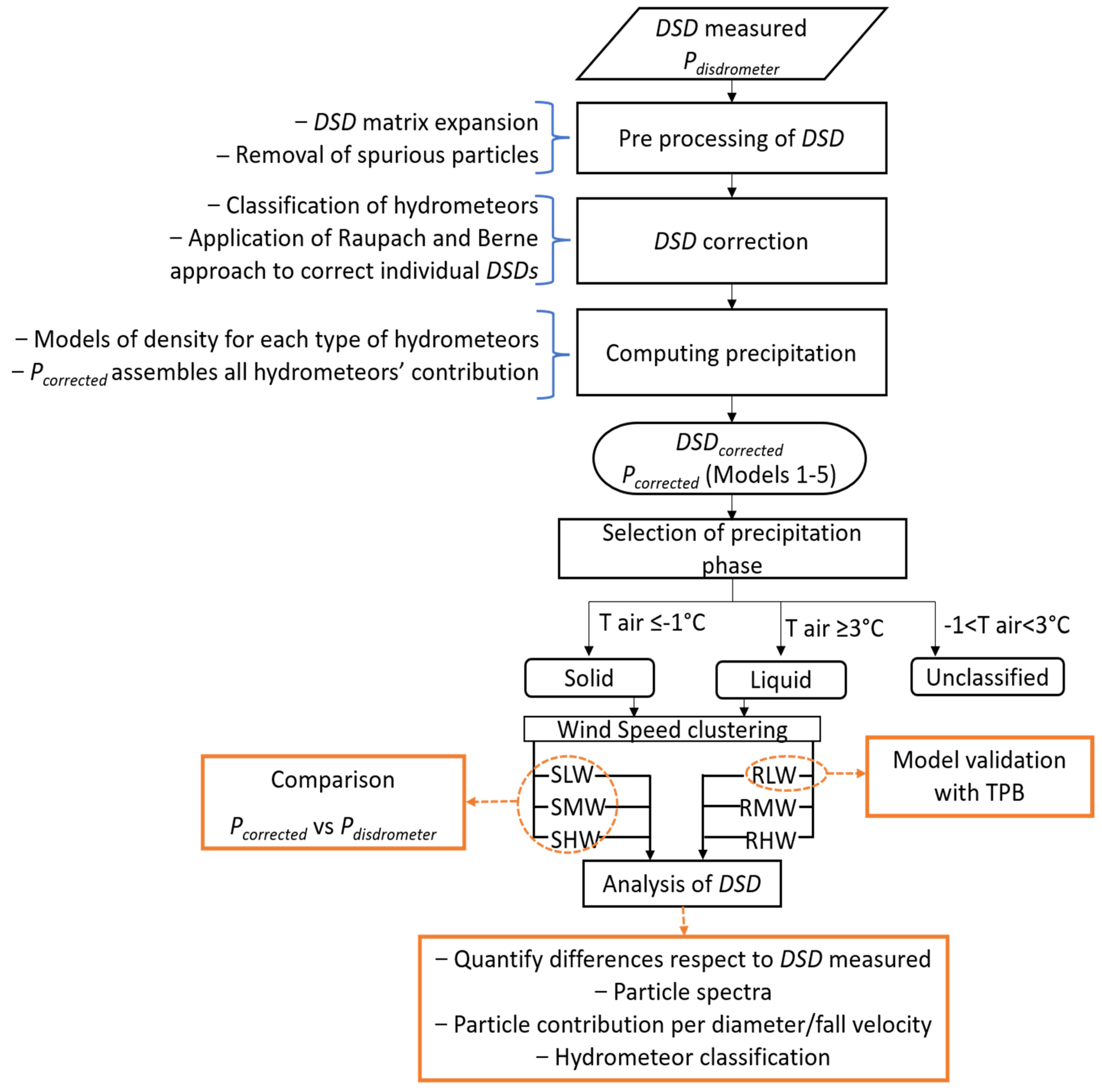
Continuous monitoring was performed between 13 July 2019 and 27 July 2020 (380 days). During this period, there were gaps only between 22–23 November 2019, due to routine maintenance and replacement of the anemometer out of order. To fill gaps of wind speed between 13 July and 23 November 2019, the measurements performed with the same type of anemometer at the ORE AWS were used. This station is located at 4850 m asl in the northwestern flank of the Antisana volcano (Figure 1b). Despite the differences in altitude and orientation, both locations showed a good correlation (r² = 0.82) and statistical significance (p < 0.01) at daily timescale for the 233 measurements available between 24 November 2019, and 27 July 2020. This ensured the reliability for fill the gap with the AWS ORE wind speed. Inspecting T_a and RH, values were within range and no corrections were applied.

Conversely, disdrometer data were filtered in order to remove erroneous measurements quoted by status flags and those with errors in DSD storage. Only measurements with both bulk variables and correct DSD measurements available were retained. Besides, trace amounts of precipitation with a rain rate less than 0.01 mm h⁻¹ were discarded in order to remove suspicious particles originated from instrument noise or dust particles [30]. Apart from 15 min measurements, we averaged meteorological conditions and integrated the DSD to obtain 30- and 60-min values, which will serve to assess the corrected precipitation over different time steps of aggregation.

3. Methods

3.1. Pre-Processing of Diameter Size Distributions (DSD)

3.1.1. DSD Matrix Expansion

Before applying a finer velocity, correction is mandatory to resize the original matrix of 32 × 32 (diameters × velocities) to 32 × 224 (diameters × velocities). This means that the diameter bins were kept unchanged, whereas the velocity bins were expanded. The first 10 velocity class bins remained the same as the original because their width is thinner than 0.1 ms⁻¹ [44]. In contrast, the velocity class bins from the 11th to 32nd were split into bins of 0.1 ms⁻¹ width. In order to redistribute the number of particles, random integers following the Latin-Hypercube method [48] were generated. Then, the original number of hydrometeors per bin was rearranged into the expanded vector. This procedure was repeated 100 times in each original bin such that the final values of the expanded vector correspond to the integer part of the average in this assemble. The non-integer difference was added to the central element of each vector keeping the sum of elements unchanged [25].

3.1.2. Diameter Based DSD Filtering

In order to remove hydrometeors that suffered deviations in their fall path to the ground, an adapted procedure using a chain of filters (F) is proposed as follows:

• F1: The particles with diameter D < 0.25 mm were removed because they are outside the sensitivity range of the instrument due to their low signal-to-noise ratio [17].
• F2: Measurements during high wind speeds are prone to particles misclassification causing large particles of DSD to appear with slow fall velocity. Therefore, particles with D > 10 mm and v < 1 ms⁻¹ were removed as suggested by Friedrich et al. [24].
• F3: Particles with diameter D < 2 mm and fall velocities 60% smaller than the fall velocity–diameter relationship of rain were removed to filter hydrometeors related to splashing [24]. These particles would have hit the housing of the disdrometer, breaking apart and rebounding back into the sampling area appearing as slow raindrops in the measured DSD.
• F4: Finally, particles with D > 20 mm were also removed because storms with large hail are more recurrent in mid-latitudes and rarely occur in the tropics [49]; therefore, the last two diameter bins were left empty.

3.2. Correction of DSD

3.2.1. DSD Decomposition

The Antisana area, due to its location on the equator, is exposed to strong daily variations in temperature and humidity [37,40]. These changes influence theirvertical profiles and modify the height of the 0 °C isotherm [50] driving phase changes that originate different types of hydrometeors [51]. Since the site is located near the 0 °C isotherm, this suggests that precipitation may be composed of a mixture of several types of hydrometeors, and the proportion of which will depend on meteorological conditions [52]. Different hydrometeor types thus may coexist for the same diameter.

Therefore, it is necessary to decompose the filtered DSDs into individual DSDs for each hydrometeor type before applying any diameter-based correction. First, the fall velocity–diameter relationship was calculated for raindrops (R), snow (S), wet snow (WS), graupel (G), lump graupel (LG), soft hail (SH), fresh hail (FH), and lump hail (LH). The relationships and diameters selected (

Table 2. Diameter range and fall velocity–diameter relationships used for the discrimination between: rain ([53], GK49; [59], AT73; [17], AM18), snow ([56], FH20; [54], LH74) wet snow (FH20), graupel (LH74), lump graupel (LH74), soft hail ([55], KN83; [24], FR13), fresh hail (KN83, FR13) and lump hail (KN83, FR13).

Type of Hydrometeor	Diameter Range (mm)	Fall Velocity (m s−1)
Rain	0.25 ≤ D ≤ 8 AM18	9.65 − (10.3 e−0.6D) GK49, AT73
Snow	0.5 ≤ D ≤ 9FH20	0.79D0.27 FH20, LH74
Wet Snow	0.5 ≤ D ≤ 9 FH20	4.65 − (5 e−0.95D) FH20
Lump Graupel	0.5 ≤ D ≤ 5 LH74	1.3 D0.66 LH74
Graupel		1.16 D0.46 LH74
Soft Hail	5 ≤ D ≤ 20 FR13	8.445(0.1D)0.553 KN83
Fresh Hail		12.43(0.1D)0.5 FR13
Lump Hail		10.58 (0.1D)0.267 KN83

) were based on the most common formulations for these hydrometeors found in the literature [24,53,54,55,56]. A correction factor was applied to the fall velocity values in order to consider the velocity increase caused by the decrease in air density [57]. This correction was calculated for the pressure (562 hPa at 4730 m asl), and the values of air temperature and relative humidity of the site according to Foote and Dutoit [58] and Atlas et al. [59].

Then, we classified the particles of the DSD according to their fall velocity and diameter. For this purpose, we computed the absolute value of the difference between the corresponding velocity class of the bin and the determined by the fall velocity–diameter relationship for the eight types of hydrometeors. In this step, only hydrometeors type inside each diameter range were considered (Table 2). The particles were allocated into the type of hydrometeor that minimized the above-mentioned absolute difference. To reduce the possibility that spurious raindrops and splashing raindrops were classified as graupel or hail in the comparison, the following preferred search order was assigned: rain, wet snow, lump graupel, graupel, snow, lump hail, fresh hail, and soft hail. This process was repeated for all bins of the expanded DSD such that the individual DSDs of each hydrometeor type was composed of particles that fell as close to their expected velocity as possible.

3.2.2. Velocity Class per Diameter Shifting

Once the individual DSDs of each hydrometeor type were obtained, we followed Raupach and Berne [25] to shift the recorded particles for each particle diameter class such that the mean velocity (from all velocity classes) aligns with the expected value according to the fall velocity–diameter relationship for each type of hydrometeor. This led to shifting each column up or down according to the difference between the mean fall velocity per diameter and the expected value.

Afterward, particles that fell through the edges of the sampling area appeared as faster or slower than the corresponding value for their fall velocity–diameter relationships. To avoid misinterpretation between splash-generated particles or fast rain particles, an additional filter (F5) was applied to remove particles outside the ±60% of the expected fall velocity according to each hydrometeor type [20,23]. Thus, the sum of all particles removed by filters F1 to F5 is represented by the net filter FT, and the “DSD corrected” resulted from regrouping the individual corrected DSDs for each type of hydrometeor. Finally, to return this DSD from the extended dimension to the original 32 × 32 diameter–velocity classes, we merged the particles in the bins corresponding to the original velocity ranges at each diameter. In the section Results, we will analyze the structure of corrected DSD through particle spectra, mean particle contribution per diameter, per fall velocity bins, and also, we will account for the hydrometeors type contribution for solid and liquid precipitation.

In order to measure the difference of particles in DSD corrected after applying the filters/corrections, we computed the difference matrix (DSD_dif) between the DSD measured by the disdrometer minus the corrected one. From this matrix, its Euclidean norm was calculated, and then the logarithm was applied to obtain the logNorm transform (Equation (3)).

$$logNorm=lo{g}_{10}DS{D}_{dif}=lo{g}_{10}\left(\sqrt{{\displaystyle \sum }_{i,j}{\left(n_{i,j}corrected-n_{i,j}measured\right)}^2}\right)$$

(3)

3.3. Calculation of Precipitation Rate

The drop concentration per unit of volume for the i-th discrete diameter class, N (D_i) (m⁻³ mm⁻¹) is defined by Equation (4). Where ∆D_i represents the interval width of each bin centered at D_i (mm), v_j is the central velocity of the j-th velocity class of DSD, and ∆t is the sampling interval generated every time step (e.g., ∆t = 900 s for 15 min). A_i (m²) corresponds to the adjusted effective sampling area for each diameter class D_i calculated by Equation (1), and n_i,j represents the number of particles in the i-th diameter class and j-th velocity class.

$$N\left(D_i\right)={\displaystyle \sum }_j\frac{n_{i,j}}{v_j}\frac{1}{A_i\Delta D_i\Delta t}$$

(4)

N(D_i) allows defining the precipitation rate (mm h⁻¹) for each type of hydrometeor R_hydrometeor by Equation (5) [60]. With a, and b the constants of the density-diameter relationships expressed by the power-law ρ = aD^b (g cm⁻³).

$$R_{hydrometeor}=6a\pi {10}^{-4}{\displaystyle \sum }_{i=1}^{32}{D}_i^{3+b}v\left(D_i\right)N\left(D_i\right)\Delta D_i=6a\pi {10}^{-4}{\displaystyle \sum }_{i,j}\frac{n_{i,j}{D}_i^{3+b}}{A_i\Delta t}$$

(5)

For raindrops, the water density 1 g cm⁻³ is broadly used, whereas density values are reported in the literature for the other hydrometeors, for snowflakes are known the relationships derived by Brandes et al. [61] and Yu et al. [62] from Parsivel measurements. For wet snow a constant value of 0.2 g cm⁻³ was reported by Zawadzki et al. [63]. Heymsfield and Wright [64], and KN83 reported 0.31 and 0.44 g cm⁻³ values for graupel and lump graupel, whereas Pruppacher and Klett [45] reported 0.5 and 0.7 g cm^−3, respectively, for soft hail is known the 0.61 g cm⁻³ value from KN83, and for lump hail had been reported 0.82 g cm⁻³ from KN83 and 0.91 g cm⁻³ from Knight et al. [65]. The fresh hail density was reported between 0.61 g cm⁻³ from KN83 and 0.7 g cm⁻³ from List [66]. In view of the above, we built 5 Models to encompass the reported values for each type of hydrometeor. Models 1 to 4 employ a combination of different values of density, while Model 5 assumed a constant density 1 g cm⁻³ for all hydrometeors.

Table 3. Set of density values (in g cm⁻³) for each type of hydrometeor in proposed models. For models 1–4, we applied the snow density-diameter relationships reported by Brandes et al. [61] (BR07) or Yu et al. [62] (YU20), while a constant value was assumed for the other hydrometeors. Model 5 assumed the density of all hydrometeors equals water density (1 g cm⁻³). Thus, the given values represent the a-parameter along with b = 0 fulfill the power-law expression ρ = aD^b.

	M1	M2	M3	M4	M5
Rain	1	1	1	1	1
Snow	YU20	BR07	YU20	BR07	1
Wet snow	0.2	0.2	0.2	0.2	1
Lump graupel	0.7	0.7	0.44	0.44	1
Graupel	0.5	0.5	0.33	0.33	1
Soft hail	0.61	0.61	0.61	0.61	1
Fresh hail	0.7	0.7	0.61	0.61	1
Lump hail	0.91	0.82	0.9	0.82	1

shows the set of the values chosen. The total precipitation rate (R_corrected) results from the total contribution of all types of hydrometeors according to each density model. The amount of precipitation is calculated by $P_{corrected} \left(mm\right)=R_{corrected}\Delta t_h$ with $\Delta t_h$ the sampling interval (in hours) (e.g., $\Delta t_h=0.25$ for 15-min records).

To assess the performance of corrected precipitation ($P_{corrected}$) with five models, we use the correlation coefficient (r²), and the root mean square error (RMSE) to check variability and residual errors with respect to reference measurements ($P_{reference}$). We also compared the accumulated $P_{corrected}$ respect to the accumulated $P_{reference}$ during available records and different wind speed regimes to obtain the relative difference (Diff) (Equation (6)) and the accumulated ratio ($A{c}_r$) (Equation (7)) in order to quantify the cumulative deviation.

$$Diff=\frac{\sum P_{corrected}-\sum P_{reference}}{\sum P_{corrected}}$$

(6)

$$A{c}_r=\frac{\sum P_{corrected}}{\sum P_{reference}}$$

(7)

As we stated in the Introduction section, we used measurements from the tipping bucket gauge (TPB) as a reference to compare low and medium wind speed records for liquid precipitation, while for the solid precipitation case, we used the Parsivel uncorrected measurements as a reference to compare the corrected solid precipitation since other measurements are not available.

3.4. Selection of Precipitation Types

The changes in temperature during precipitation events result in a transition between different phases [52,67]. Such transitions are more complex in alpines zones like the Inner Tropics where the temperature seasonal cycle is weak (Figure 2). For this reason, this study focuses on instantaneous records of solid, liquid, and unclassified precipitation instead of an event-wise analysis. To distinguish between solid and liquid precipitation phases (PP) we followed the work of Wagnon et al. [68]. Precipitation records with T_a ≤ −1 °C are considered as solid (PP = 0), and those with T_a ≥ 3 °C were considered as liquid precipitation (PP = 1). These temperature thresholds were derived through field observations and meteorological measurements at AWS ORE (Figure 1). The measurements between −1 and 3 °C correspond to unclassified precipitation type records which need further filters to ensure accurate phase forecasting. For this reason, only the DSDs corresponding to solid and liquid precipitation will be analyzed.

In addition, the precipitation types reported by the disdrometer through the SYNOP Code of Table 4680 [44] were related to a disdrometer precipitation phase (DPP). For instance, drizzle (cods = 51, 52, 53), drizzle-rain (cods = 57, 58, 59) and rain (cods = 61, 62, 63) were considered as rainfall, DPP = 1. Snow (cods = 71, 72, 73) and snow grains (cods = 77) were classified as snowfall, DPP = 0, whereas records detected as soft hail (cods = 87, 88), hail (cods = 89, 90) and rain-snow mixture (cods = 67, 68, 69) were taken as mixed precipitation, DPP = 0.5. Thus, we define a match record when DPP and PP coincided (i.e., PP and DPP = 0 for solid precipitation, similarly with PP and DPP = 1 for liquid precipitation). In contrast, a misclassified record corresponds to a mismatch (i.e., PP = 1 and DPP = 0 or 0.5, the same to PP = 0 for DPP = 1 or 0.5).

Since the type of precipitation is determined based on the size and typical speeds [17,44], there is a possibility that a small contribution of particles in the DSD can come from different hydrometeors. Therefore, the DSD of liquid precipitation based on the 3 °C threshold can include a small percentage of particles classified as snow, graupel, or hail according to the fall velocity–diameter relationship. Similarly, solid precipitation based on the −1 °C threshold can include a small contribution of particles classified as raindrops.

3.5. Clustering of Solid and Liquid Precipitation by Wind Speed

Once the records of solid and liquid precipitation were identified, the unsupervised learning clustering approach, k-means [69] was applied on the associated meteorological variables. For partitioning the records of the two sets, we used the meteorological variables: Air temperature (T_a), Dew point temperature (T_d), Specific humidity (q), and Wind speed (Ws). The number of groups to cluster solid and liquid precipitation was obtained by maximizing the silhouette criterion [70]. Considering this study aims to evaluate the impact of the correction for different wind speeds, the mean group values of Ws were used to identify low, mid and high wind speed regimes for both phases at which precipitation occurs.

Figure 3 summarizes the procedure described in the methodology. After pre-processing and applying DSD corrections, the precipitation was computed. Then, we classified records by air temperature into solid and liquid phases. Then, we applied the wind speed-based clustering to identify distinct regimes in order to reveal the differences in DSD and between corrected and measured precipitation.

4. Results

4.1. Solid and Liquid Precipitation

A summary of the data acquired by the Parsivel OTT² disdrometer at 15 min resolution and the corresponding cumulative values at 30 and 60 min are shown in

Table 4. Disdrometer data summary for the 15, 30, and 60 min time scales. Total number of records, errors, records with precipitation, and with precipitation rate >0.01 mm h⁻¹ are shown. The records with valid DSD and the common high-quality records containing (1) correct DSD, (2) correct bulk values, and (3) with precipitation > 0.01 mm h⁻¹ are also shown. Identified records as solid, liquid and unclassified precipitation are also included. The values in parentheses correspond to percentages of solid, liquid, and unclassified precipitation with regards to the number of records of the high-quality dataset.

Integration Time	15 min	30 min	60 min
Total records	36 496	18 248	9124
Retrieved measurements	35 603	17 769	8857
Error flags	486	118	74
Precipitation records	7776	4547	2711
Precipitation with R > 0.01 mm h−1	7724	4455	2595
Valid DSD	5004	2934	1680
Common high-quality records	4983	2876	1611
Identified Solid precipitation (Ta ≤ −1 °C)	159 (3%)	86 (3%)	40 (2%)
Identified Liquid precipitation (Ta ≥ 3 °C)	298 (6%)	217(7%)	152 (9%)
Unclassified precipitation (−1 °C < Ta < 3 °C)	4526 (91%)	2573 (90%)	1419 (89%)

. At the 15 min scale, technical problems (i.e., power supply failures and data communication problems) and erroneous measurements (i.e., reported by error flags) caused a missing of 2.4% and 1.3% of the 36 496 gathered measurements. When inspecting records with precipitation only, there were 7776 values, of which 5004 allowed us to correct recorded DSD. Thus, precipitation was present in 22% of the measurements, of which 21% corresponded to rain rates greater than 0.01 mm h⁻¹. Finally, after applying the quality data control, 4983 values with valid information for both the DSD, bulk variables and rain rates greater than 0.01 mm h⁻¹ were available. This means the common high-quality dataset, which contains the solid, liquid, and unclassified precipitation records, corresponded to 14% of the total data gathered in the one-year monitored period.

The precipitation phase selection allowed us to identify 298 records as liquid precipitation (6%), 159 as solid precipitation (3%). The remaining 4526 values (91%) corresponded to unclassified precipitation within the interval −1 °C < T_a < 3 °C. This result was expected due to the recurrent fluctuations of the 0 °C isotherm around the height of the site. The accumulation of measurements at 30- and 60-min scales reduced the high-quality records. Furthermore, the variability of temperature tends to decrease for larger time scales which hinders to have extended intervals with T_a ≤ −1 °C and reduced the number of records with solid precipitation, whereas the number of records above this threshold increased, explaining the increase of unclassified and liquid precipitation contribution (Table 4).

In addition, the DPP and the PP of the 15 min records of solid and liquid precipitation were examined (

Table 5. Comparison between the precipitation phase measured by the disdrometer (DPP) and the classified precipitation in this study. The percentages of contribution of each subgroup (LW, MW, HW) regarding liquid and solid precipitation are shown in parenthesis.

	Disdrometer Precipitation Phase (DPP)
Identified Precipitation	Snowfall	Mix	Rainfall
Liquid	73 (23.6)	46 (15.4)	179 (61)
RLW	6(4.6)	12(9.2)	112 (86.2)
RMW	26 (26)	21(21)	53 (53)
RHW	41 (60.3)	13 (19.1)	14 (20.6)
Solid	154 (96.8)	2 (1.3)	3 (1.9)
SLW	72(97.3)	1 (1.3)	1 (1.3)
SMW	56(96.6)	1 (1.7)	1 (1.7)
SHW	26 (96.3)	0 (0)	1 (3.7)

). For the solid precipitation, the disdrometer showed a hit rate of 96%, whereas for the liquid precipitation case, the hit rate was 61% on average. The air temperature and specific humidity during the records misclassified by the disdrometer were similar to those well-catalogued (

Table A1. Mean meteorological conditions for rainfall, mixed and snowfall reported by disdrometer concerning liquid and solid precipitation records.

Disdrometer Precipitation	Identified Precipitation (Based in Ta)	N	Ta (°C)	Td (°C)	q (g kg−1)	RH (%)	Ws (m s−1)
Rainfall	Liquid	179	3.63	2.26	7.93	90.97	4.19
Mix		46	3.68	0.71	7.11	81.23	6.58
Snowfall		73	3.81	0.17	6.82	77.26	9.46
Rainfall	Solid	3	−1.67	−2.38	5.72	94.9	6.71
Mix		2	−1.45	−1.70	6.01	98.15	3.53
Snowfall		154	−1.48	−1.87	5.94	97.16	3.21

). However, relative humidity and wind speed showed differences, especially in the records identified as liquid precipitation (T_a ≥ 3 °C) but reported as snowfall or mixed. This could occur because the measured particles under strong winds are prone to misclassification [24]. This affected the types of precipitation reported by the disdrometer and highlights the need to apply an additional filter to reclassify the phase precipitation in the disdrometer.

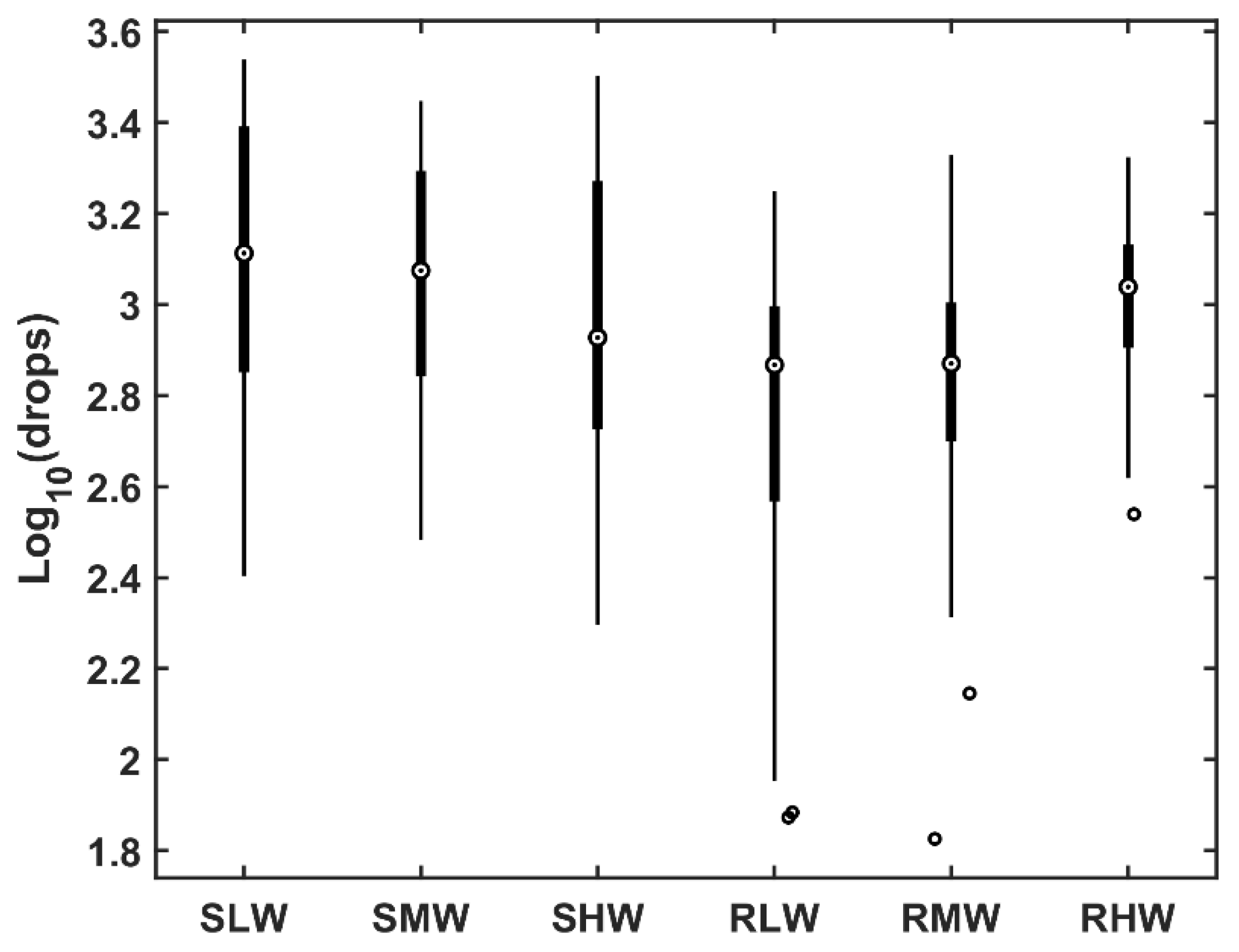
4.2. Clusters of Liquid and Solid Precipitation according to the Wind Speed Regime

The Silhouette criterion suggests 2 clusters for both solid and liquid precipitation by using the k-means technique. Nevertheless, the Ws differences between clusters’ centers were around 3.5 m s⁻¹ for solid and 7.5 m s⁻¹ for liquid precipitation as a consequence of its large variability (Table 1). This means that the harsh environmental conditions prevent obtaining measurements without disturbances. Thus, the number of groups was manually set to three in order to obtain an intermediate cluster of wind regimes. Clusters are hereafter referred to as low, medium, and high Ws regimes. The clusters’ centers are shown in

Table 6. Cluster means of solid and liquid precipitation records estimated at 15 min time scale by using K-means. N represents the number of records per group, parentheses are show the contribution for each phase respectively.

Precipitation Phase (Based on Ta)	Cluster	N (%)	Ta (°C)	Td (°C)	q (g kg−1)	RH (%)	Ws (m s−1)
Liquid	RLW	130 (44)	3.57	2.32	7.96	91.67	2.62
	RMW	100 (35)	3.66	1.3	7.41	84.88	5.92
	RHW	68 (20)	3.93	0.28	6.87	77.32	11.93
Solid	SLW	74 (47)	−1.39	−1.63	6.05	98.35	1.74
	SMW	58 (36)	−1.57	−2.04	5.87	96.64	3.68
	SHW	27 (17)	−1.5	−2.22	5.79	94.9	6.53

, which are interpreted as the more equidistant between Ws means according to the Euclidean distance. The resulting clusters for solid precipitation were renamed as solid with high wind (SHW), solid with moderate wind (SMW), and solid with light wind (SLW). While for liquid precipitation, we obtain liquid precipitation with high wind (RHW), liquid precipitation with moderate wind (RMW), and liquid precipitation with light wind (RLW).

Light wind records (RLW + SLW) accounted for the 45% of all analyzed records (Table 6). Moderate wind speed constituted about 35%, and high wind speed records accounted for the remaining 20%. The performance of the disdrometer for the three solid precipitation groups was good and achieved hit rate values greater than 95% (Table 5), suggesting that the low temperature threshold of −1 °C performs well for discriminating solid precipitation. For liquid precipitation the hit rate was 86% for RLW. For RMW this score decreased to 53% together with a reduction of T_d and q. The RHW displayed a hit rate of 20% with a drop in q below 7 g kg⁻¹ and T_d near to 0 °C (Table 6). These highly variable conditions during liquid precipitation could limit the disdrometer performance to wind speeds lower than 6 ms⁻¹ and RH over 85%.

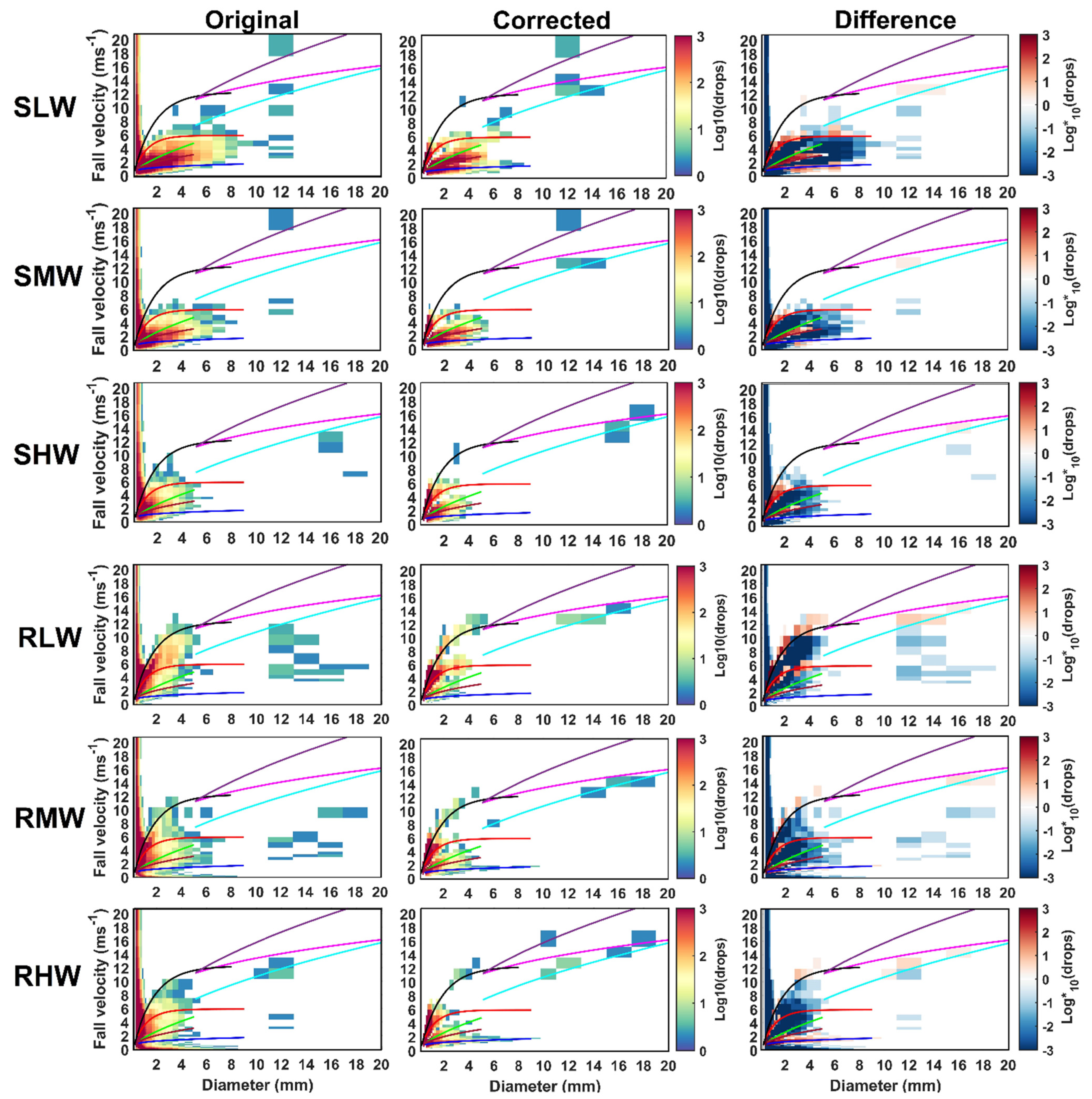
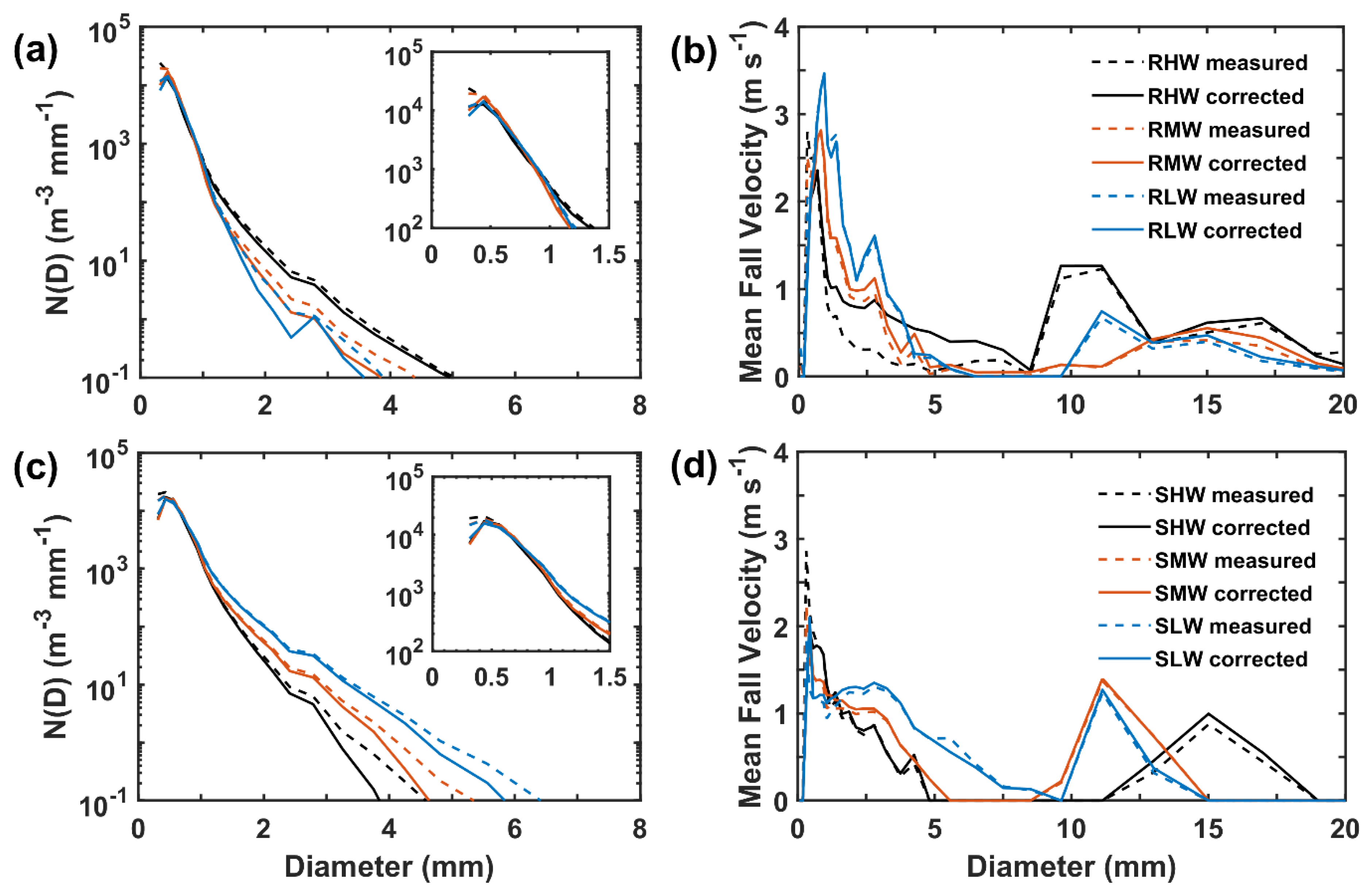
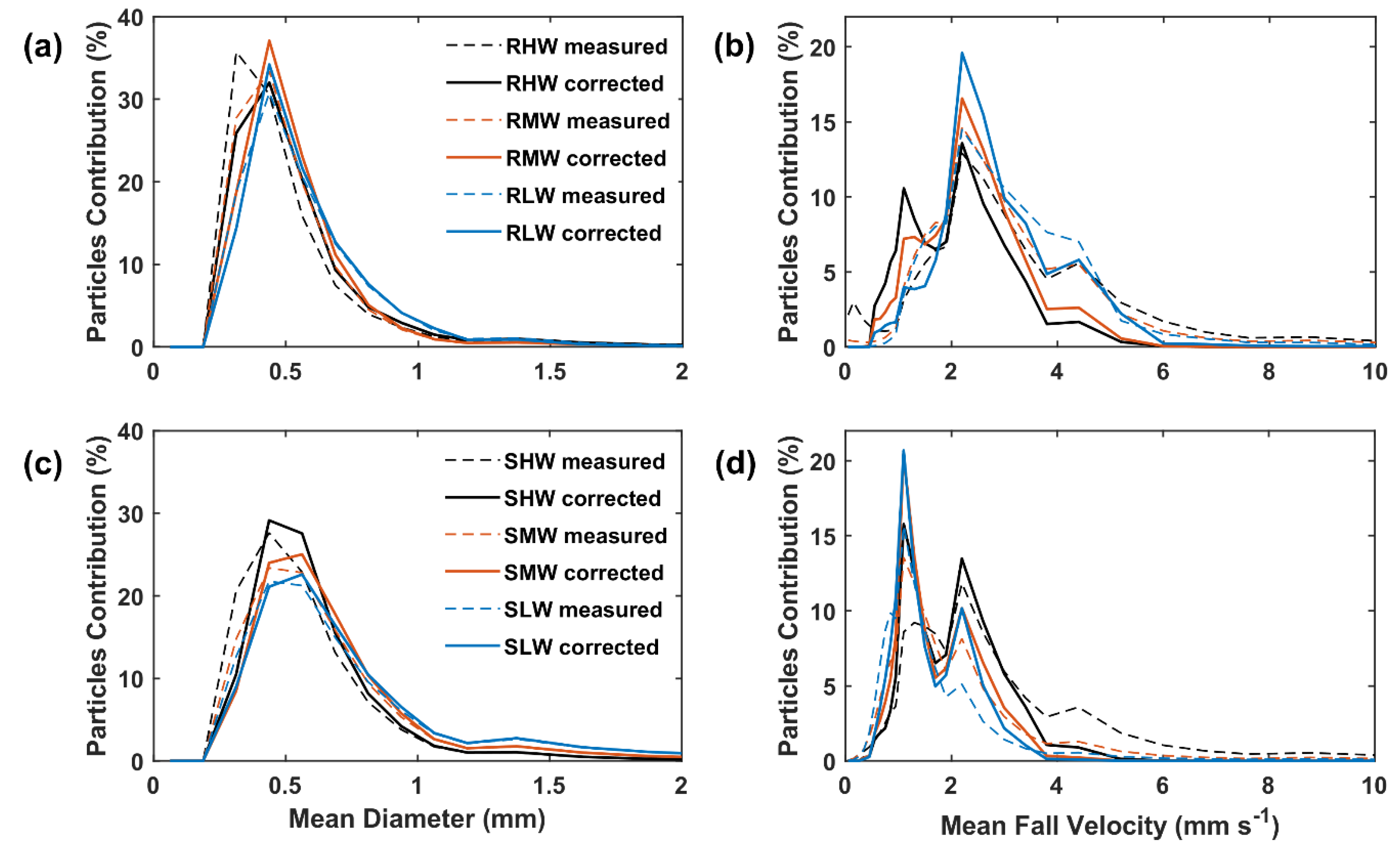
4.3. The Corrected Drop Size Distributions (DSDs)

In this section, we compared the changes of DSD after the implementation of filters and corrections described above. We also compared the differences between corrected solid and liquid DSDs. We skipped unclassified precipitation to simplify the analysis. Almost all particles of liquid precipitation had diameters D ≤ 8 mm between rain and snow curves, and a negligible contribution of hail (<1%) had diameters between 12 and 20 mm. Similarly, it occurred for solid precipitation, where most particles’ diameters span the area comprised between the curves of wet snow and snow (Figure 4). Filters primarily removed particles with D ≤ 1 mm that are faster than the fall velocity–diameter relationship of rain, wet snow, and wet graupel (F5). This was more frequent in RHW, RMW, and SHW subgroups (

Table 7. Mean percentages of removed particles by each filter applied in each group respect to measured DSDs. To account the changes of DSDs after filters/corrections, the mean logNorm value and the mean number of particles before and after corrections were included.

	Particles Filtered (%)						logNorm (log (Particles))	Number of Particles
	F1	F2	F3	F4	F5	FT		Measured	Corrected
Rain	1.8 × 10−4	4.4 × 10−4	0.74	1.4 × 10−4	11.56	12.3	2.85	1.01 × 104	9.34 × 103
RLW	2.9 × 10−4	6.2 × 10−4	0.24	0	5.62	5.12	2.77	9.68 × 103	8.91 × 103
RMW	1.1 × 10−4	4.6 × 10−4	0.83	2 × 10−4	14.06	11.23	2.84	1.09 × 104	1.02 × 104
RHW	0.7 × 10−4	3.2 × 10−4	1.55	3.2 × 10−4	19.25	18.36	3.01	9.29 × 103	8.97 × 103
Snow	0	2.1 × 10−4	4.25	0	7.02	11.28	3.04	1.82 × 104	1.65 × 104
SLW	0	2.8 × 10−4	5.11	0	4.49	9.61	3.08	1.91 × 104	1.71 × 104
SMW	0	0	3.92	0	7.44	11.36	3.04	1.78 × 104	1.63 × 104
SHW	0	0	2.62	0	13.07	15.69	2.96	1.66 × 104	1.55 × 104

) because wind speeds were higher than 5.92 m s⁻¹. Filters also removed particles of solid precipitation and RHW that passed through the sampling area with D ≤ 2 mm and velocities lower than 2 ms⁻¹ as a consequence of splashing effects. Inspecting the DSDs (Figure 4), there were scarce and probably unrealistic particles with D ≥ 10 mm and v ≤ 1 ms⁻¹ and few particles with D ≥ 20 mm or D ≤ 0.025 mm, which caused low percentages of particles removed (<0.001%). Hence, the removal produced by filters F1, F2, and F4 were negligible for both precipitation phases.

In effect, the corrections removed around 5% of the particles in the DSDs of the RLW group and promote the particles to align around the empirical curves employed. The particles of resulting DSDs present two regions of preference, one zone with particles with D ≤ 6 mm around the rain curve and another with D ≤ 4 mm around the wet snow curve. Particles with D ≥ 10 mm and v ≤ 6 ms⁻¹ were removed, and a small fraction of particles (<1%) with v ≥ 8 ms⁻¹ were aligned with the soft hail curve. In the RMW group, the corrections removed 11% of the total particles and generated a distribution similar to RLW. The particles with v ≥ 6 ms⁻¹ were aligned around the rain curve, whereas particles with v ≤ 6 ms⁻¹ aligned around wet snow and wet graupel curves. The DSDs of the RHW group were the most affected by the filters, particularly, F5 removed 19% of fast particles due to margin faller effects enhanced by the wind speed increase [24,71]. Therefore, the corrected DSD was narrow with diameter–velocity of particles concentrated up to D ≤ 4 mm and v ≤ 6 ms⁻¹.

Conversely, the DSDs of solid precipitation had a broader diameter spectrum (D ≤ 10 mm) with particles’ diameter–velocity mainly concentrated between wet and snow curves. Flow distortions around an exposed gauge device (like disdrometer) are proportional to wind speed [11,42]. Thus, the increase of wind speed caused more snowflakes to be deflected [15], reducing the frequency of direct collision to disdrometer housing and splashing effects. Therefore, the F3 filter removed more particles related to the splashing effect in SLW than SMW and SHW. The same snowflake deflection justifies the increase of fast particles removed by F5 in SMW and SHW respect SLW (Table 7). Both filters affected mainly SHW records which had narrow DSDs with particles up to 4 mm in diameter, while SLW had particles up to 9 mm. As consequence, the corrections/filters also forced solid precipitation DSDs to follow a bimodal distribution. One zone was around the rain and wet snow curves with D < 4 mm, and the second zone was around wet graupel and snow curves.

Furthermore, Figure 5 shows the boxplot of the logNorm values calculated for each phase’s subgroup in order to quantify the differences in DSDs produced by corrections. SLW had the greater values because this subgroup has the greater number of particles despite all filters FT removed 9.6% of measured particles. Hence, the difference was the largest, contrary to RHW which achieved the largest filtered percentage but had the lowest number of particles (Table 7). Consequently, DSDs of solid precipitation records were the most affected by the corrections than liquid precipitation, and precipitation with high wind speed (RHW and SHW) were more prone to corrections as was expected.

4.3.1. Characteristics of Corrected DSD

Figure 6 shows the average particle concentration spectra for liquid and solid precipitation. The DSDs of RLW, RMW, and RHW had an initial maximum concentration at a diameter of 0.31 mm; after corrections, this peak shifted towards 0.44 mm. As diameter increases, the concentration for larger particles dropped abruptly up to 3.75 mm for the RLW group. In RMW and RHW this decrease in concentration was damped to particles with diameters 4.25 and 5.5 mm respectively. For solid precipitation groups, the filters remove the fast particles with diameters 0.31 mm that reduced their initial concentration. For particles between 0.43 ≤ D ≤ 1 mm, the concentration of corrected DSDs was similar to the measured. The filters removed particles with larger diameters than D > 1 mm, which decreased particle concentrations regarding the values measured. This difference was more noticeable in SHW where the particle concentration dropped quickly after the peak at 0.44 mm with respect to SMW and SLW which retained particles with diameters larger than 5 mm. Thus, liquid precipitation DSDs were mostly concentrated up to diameters 3.75 mm, while in solid precipitation having particles with diameters up to 6 mm was possible. After these diameters, their concentration spectra were lower than 0.1 mm⁻³ mm⁻¹ and were not considered.

Moreover, the panels b and d of Figure 6 display the mean fall–velocity per diameter for the liquid and solid precipitation groups. These values resulted from averaging the fall–velocity of all particles in the corresponding diameter. Thus, the low fall–velocity of snow and graupel were compensated with the high values attained by rain and hail hydrometeors (Figure 4). The DSDs of liquid precipitation exhibit a peak of velocity frequencies around 2.5–3.5 ms⁻¹, corresponding to particles with 0.5–1.2 mm diameters and another peak around 1–1.5 ms⁻¹ for particles with diameters between 1.9–2.5 mm, in agreement with the bimodal distribution around the rain and wet snow curves (Figure 4). For the solid precipitation DSDs, the fall speed peaks around 2–2.5 ms⁻¹ for particles with diameters of 0.44–0.56 mm corresponding to melting snow and rain particles. The region within 0.56 ≤ D ≤ 2.5 mm showed mean fall speed around 1.25 ms⁻¹, which could correspond to wet snow or graupel particles, whereas for particles within 2.5 < D ≤ 5 mm this value decreased to around 0.5–1 ms⁻¹ in agreement with the fall velocity–diameter relationship of snow. For D ≥ 8 mm in both solid and liquid groups, there was a sudden fall speed rise related to the presence of soft and lump hail particles.

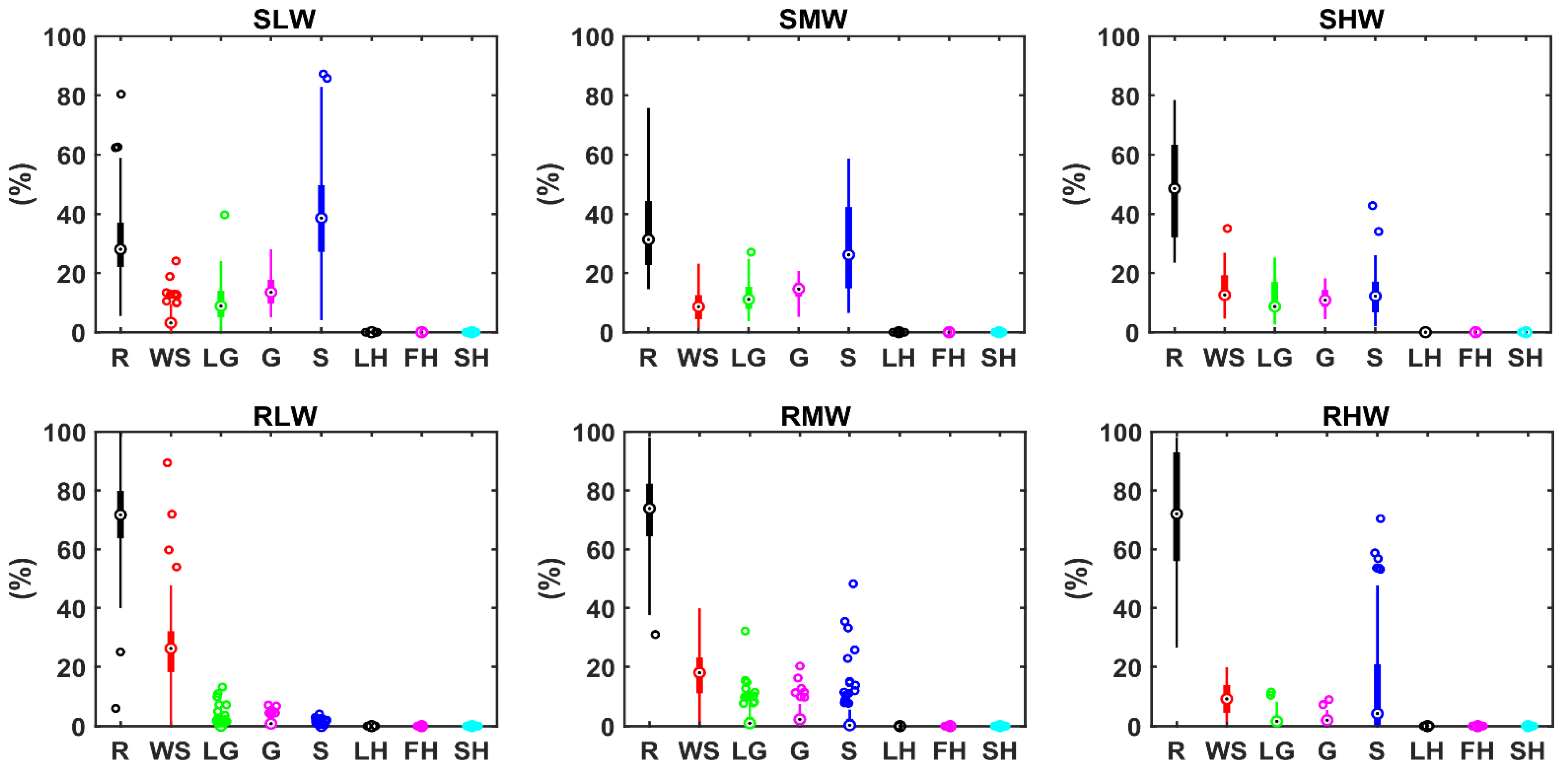
4.3.2. Composition Analysis of Corrected DSD

The major contribution by diameter in DSD occurred at 0.44 mm (Figure 7), which allowed us to confirm that the particles’ diameter follows a unimodal distribution, in agreement with the concentration spectra displayed in Figure 6. The 99% of DSD was composed of particles up to 1.2 mm for liquid precipitation and up to 1.63 mm for the solid case. DSDs with high wind speed (RHW and SHW) were concentrated between 0.31 ≤ D ≤ 0.81 mm, contrary to DSDs with low wind speed that had broader spectra. This could occur because the wind enhanced the collisional breakup process, reducing the concentrations of larger particles and modifying the DSDs [72].

Conversely, the fall speed of liquid precipitation follows a trimodal distribution, with a major peak at 2.2 ms⁻¹ corresponding to 0.44 mm diameter, which constitutes the highest concentration (Figure 6a) and in turn the largest diameter contribution (Figure 7a). The other two peaks correspond to 1.1 ms⁻¹ and 4.4 ms⁻¹ due to the concentration of particles around the values in the snow and wet snow curves, respectively (Figure 4). Conversely, the mean fall speed per diameter bins of solid precipitation DSDs followed a bimodal distribution. The first peak at 1.1 ms⁻¹ resulted from the particle concentration around the theoretical snow curve (SLW and SMW in Figure 4) that converged toward that value. The second peak occurred at 2.2 ms⁻¹, corresponding to the rain fall velocity–diameter relationship for D = 0.44 mm in agreement with the maximum particle concentration (Figure 6c) and contribution (Figure 7c). The concentration of particles with D > 2 mm was less than 10 particles m⁻³ mm⁻¹ for solid and liquid cases (Figure 6a,c), explaining the negligible diameter contribution beyond 2 mm and the slight velocity contribution beyond 5 m s⁻¹ in Figure 7.

Similarly, the decomposition of the measured DSDs (Section 3.2.1) allowed us to quantify the percentage contribution of each type of hydrometeor (based on the fall velocity–diameter relationship) for each subgroup (Figure 8). In general, the DSDs of solid precipitation records contain 48% of raindrops and 52% of solid hydrometeors distributed among snow (17%), graupel (15%), wet snow (11%), and wet graupel (9%). In SLW, precipitation was composed of rain (28%), snow (39%), graupel (22%), and wet snow (11%), whereas in SMW and SHW, the proportion of raindrops (40%) and wet snow (12%) increased, and the snow (19%) and graupel (12%) contribution decreased. These changes in hydrometeors proportions could be related to the breakup of larger hydrometeors with D > 2 mm induced by the wind speed increase [72]. Especially in SHW, the concentration of small particles with D < 0.8 mm accounted for 90% of DSD (Figure 6). In contrast, liquid precipitation DSDs were mainly composed of raindrops and wet snow particles. In RLW, these hydrometeors contributed with 71% and 27% of the total precipitation, whereas, for RMW and RHW the increase in wind speed could favor the breakup and also the melting of snowflakes [73] which decreased the contribution of wet snow to around 14%.

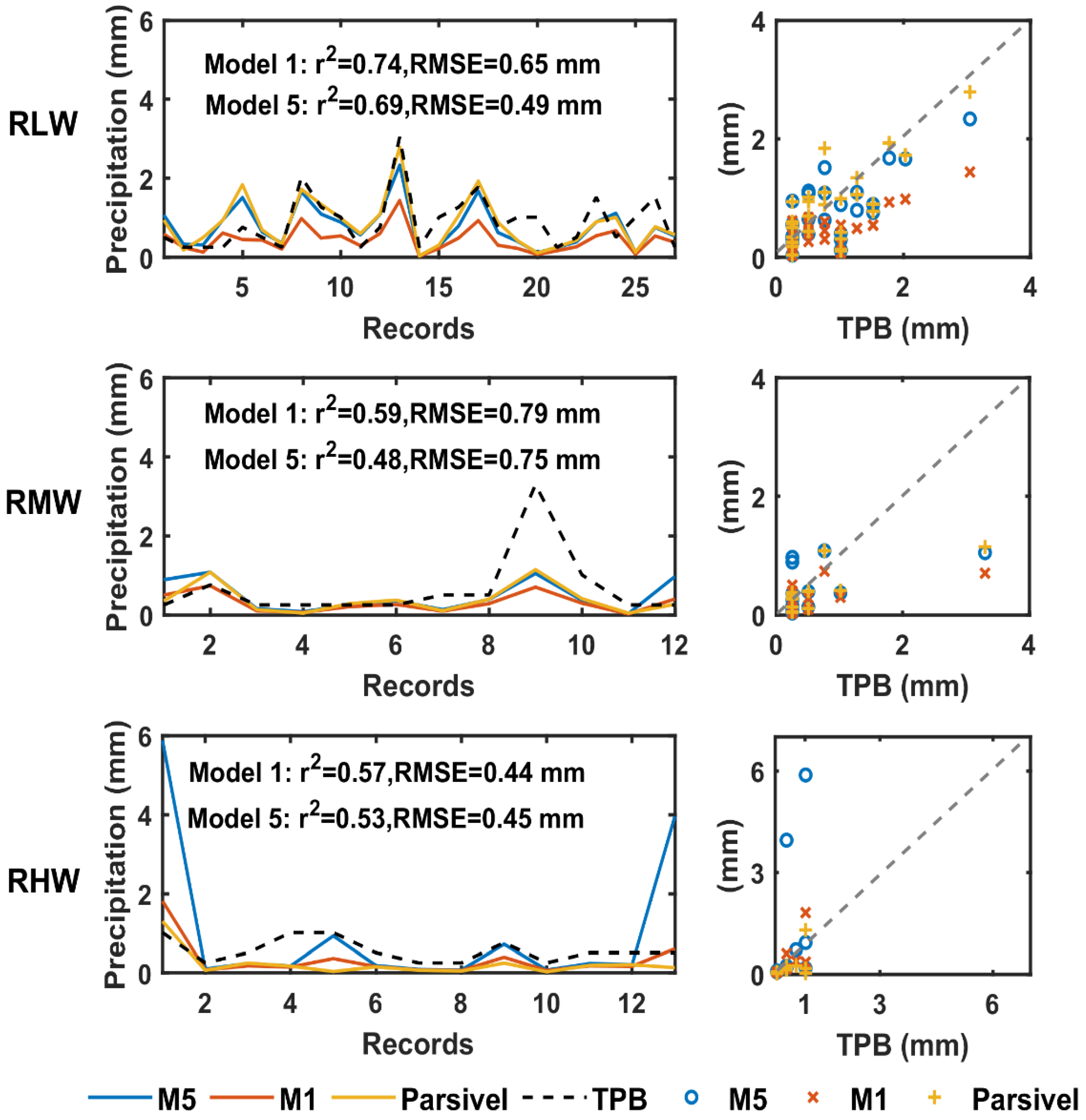
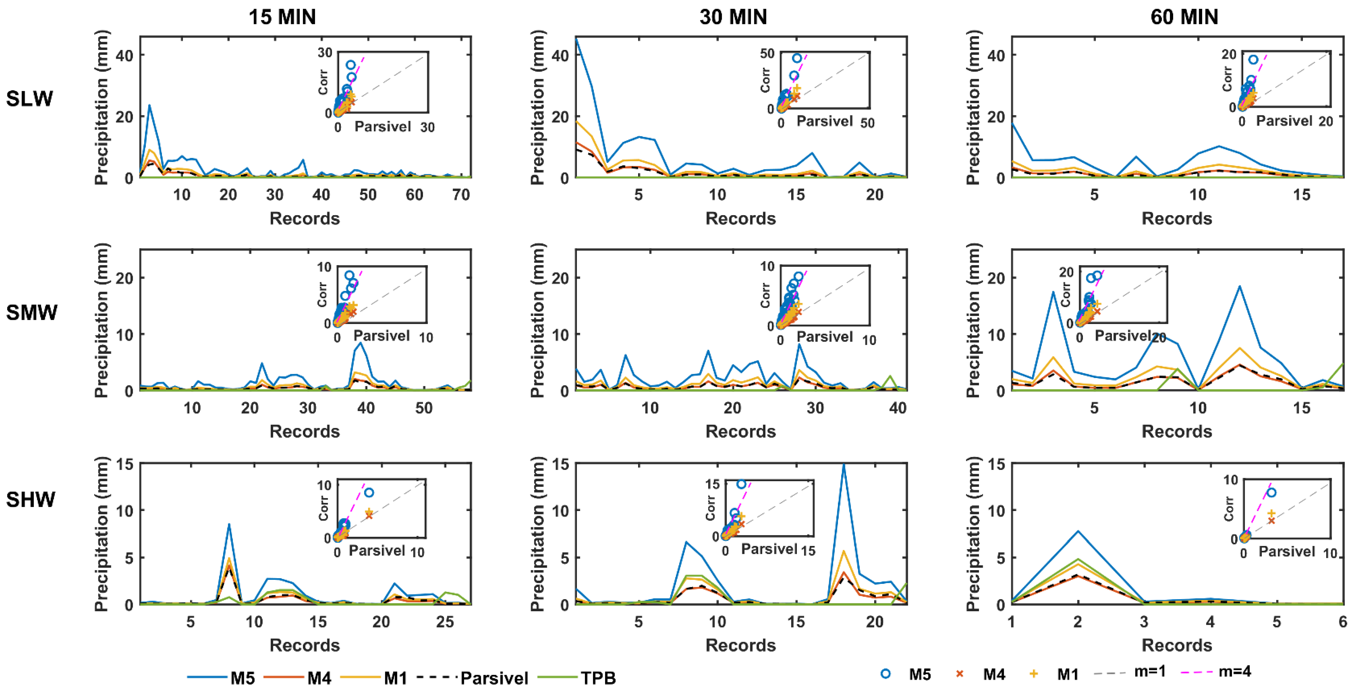
4.4. Corrected Precipitation according to Particle Density Models

To assess corrected precipitation obtained through the five density models (Section 3.3), we compare the corrected values for liquid precipitation with respect to TPB as reference. We first focus on records under the low wind speed regime (RLW) to ensure reliable measurements and to avoid the under-catch effect. For the 15 min records, all models exhibit negative relative differences (Diff in

Table 8. Coefficient of correlation (r²), RMSE, relative difference (Diff) and accumulated ratio (Ac_r) between corrected precipitation following the five density models and TPB precipitation for 15, 30, and 60 min timescales. Scores are displayed for low (RLW), moderate (RMW), and high wind speed (RHW) groups and for all liquid precipitation records.

	15 min				30 min				60 min
	r2	RMSE	Diff	Acr	r2	RMSE	Diff	Acr	r2	RMSE	Diff	Acr
	RLW
M1	0.18	0.44	−0.61	0.39	0.56	0.54	−0.51	0.49	0.76	0.69	−0.45	0.55
M2	0.19	0.44	−0.61	0.39	0.56	0.54	−0.51	0.49	0.76	0.69	−0.45	0.55
M3	0.19	0.44	−0.62	0.38	0.56	0.55	−0.51	0.49	0.76	0.69	−0.45	0.55
M4	0.19	0.44	−0.62	0.38	0.56	0.55	−0.52	0.48	0.76	0.69	−0.45	0.55
M5	0.17	0.46	−0.35	0.65	0.58	0.47	−0.2	0.8	0.78	0.51	−0.1	0.9
	RMW
M1	0.42	0.36	−0.54	0.46	0.65	0.46	−0.49	0.51	0.68	0.73	−0.38	0.62
M2	0.42	0.36	−0.56	0.44	0.66	0.46	−0.50	0.50	0.69	0.73	−0.40	0.60
M3	0.43	0.36	−0.57	0.43	0.66	0.47	−0.53	0.47	0.69	0.74	−0.42	0.58
M4	0.42	0.37	−0.59	0.41	0.65	0.48	−0.54	0.46	0.69	0.75	−0.44	0.56
M5	0.42	0.40	−0.20	0.80	0.64	0.51	−0.15	0.85	0.66	0.84	0.04	1.04
	RHW
M1	0.58	0.30	−0.43	0.57	0.59	0.51	−0.54	0.46	0.70	0.77	−0.52	0.48
M2	0.54	0.32	−0.52	0.48	0.58	0.52	−0.57	0.43	0.70	0.80	−0.55	0.45
M3	0.59	0.30	−0.45	0.55	0.60	0.51	−0.56	0.44	0.72	0.78	−0.55	0.45
M4	0.55	0.32	−0.54	0.46	0.59	0.53	−0.60	0.40	0.72	0.81	−0.59	0.41
M5	0.53	0.64	0.37	1.37	0.55	0.53	−0.27	0.73	0.67	0.74	−0.23	0.77
	Liquid Precipitation
M1	0.34	0.39	−0.55	0.45	0.59	0.51	−0.51	0.49	0.71	0.72	−0.45	0.55
M2	0.34	0.39	−0.58	0.42	0.59	0.52	−0.52	0.48	0.71	0.73	−0.46	0.54
M3	0.35	0.39	−0.57	0.43	0.6	0.52	−0.53	0.47	0.72	0.73	−0.47	0.53
M4	0.34	0.39	−0.59	0.41	0.59	0.52	−0.54	0.46	0.72	0.74	−0.48	0.52
M5	0.31	0.49	−0.15	0.85	0.58	0.5	−0.2	0.8	0.7	0.68	−0.1	0.9

) indicating that corrected precipitation underestimate the amount of precipitation. This occurs because selected records are non-continuous; thus, it was possible to introduce additional precipitation (as graupel, hail, or snowflakes) in precedent records that could be measured in the current record affecting the comparison. Similarly, the low correlations for all models occurred due to delays on the TPB suggesting that the 15 min timescale seems to be too short to derivate precipitation properly in the study site.

Therefore, we aggregated the 15 min records to 30 and 60 min temporal resolution and explore their behavior. Table 8 summarizes the scores achieved. The correlation of all models tends to be better with these datasets. All models reached correlation values greater than 0.55 and 0.75 for 30- and 60-min timescales, respectively. This can result from the necessary time for hydrometeors’ raindrops to slip from the rubber funnel until they arrive at the gauge orifice before causing tipping. Hence, longer time records compensate for the delays at 15 min, yielding an improvement in the timing detection at TPB.

Aggregating the temporal resolution also avoided disruptions in records between precipitation events since most of them surpass the 30 min at the site. Therefore, we reduced the loss of information between records. Furthermore, this minimizes the introduced solid or unclassified precipitation corresponding to precedent records. This fact can justify the reduction in the relative difference and in turn the reduction of underestimation at longer timescales for all models (Table 8). The accumulated ratio was shortened regarding the 15 min scores. The corrected precipitation with the Models 1 to 4 reached similar performance with slightly better performance of the Model 1 at 30 min records. (Table 8). M5 minimized the relative difference and maximized the correlation for the three time-scales. Figure 9 shows the series of liquid precipitation measured in Parsivel OTT² disdrometer and the values computed with density models 1 and 5 respect to TPB.

Furthermore, we examined only records without previous precipitation one hour before to reduce the possibility of measure introduced precipitation previous to the liquid records. Figure 10 shows the comparisons for M1 and M5 after this events selection at 60 min scale (following the better correlation coefficients). This imposed condition allowed to reduce the RMSE and the relative difference of both models, with M5 presenting the lowest difference for RLW. This demonstrates the delay effect of precedent time-step precipitation over current liquid precipitation records at TPB and its influence on the resulting scores.

Exploring the scores of M5 for RMW and RHW. The RMSE and Diff were the lowest, whereas the accumulated ratio Ac_r was the maximum respecting to M1-M4 scores as well (Table 8). This means that corrected precipitation with M5 densities reaches the minimum differences with respect to TPB as displayed in Figure 9 and Figure 10. M5 is thus the best model to represent liquid precipitation despite the expected undercatch greater than 23% for wind speed greater than 10 m s⁻¹ for conventional cylinder rain gauges similar to TPB [11]. Therefore, this model (i.e., the corrections applied by assuming the same density for all hydrometeors) can be employed to correct liquid precipitation as it has been reported for sites dominated by rainy conditions [25].

For the solid precipitation for the solid precipitation case, TPB did not allow to collect reliable instantaneous precipitation, and measurements did not represent the precipitation variability (Figure 10). Thus, we compare the corrected values regarding to uncorrected measurements. Comparing the corrected series with M5 with respect to the Parsivel series for SLW over different time scales (Figure 11), this density model got Ac_r between 4.1 to 4.8 (

Table 9. Root mean square error (RMSE), relative difference (Diff), and accumulated ratio (Ac_r) between precipitation corrected with five density models and Parsivel measurements for three timescales. Scores are displayed for low (SLW), moderate (SMW), and high wind speed (SHW) groups of solid precipitation.

	15 min			30 min			60 min
	RMSE	Diff	Acr	RMSE	Diff	Acr	RMSE	Diff	Acr
SLW
M1	0.84	0.71	1.71	2.49	0.88	1.88	1.15	0.88	1.88
M2	0.68	0.44	1.44	2.08	0.64	1.64	0.67	0.44	1.44
M3	0.35	0.29	1.29	0.97	0.37	1.37	0.65	0.52	1.52
M4	0.23	0.02	1.02	0.58	0.14	1.14	0.20	0.08	1.08
M5	3.49	3.08	4.08	9.80	3.60	4.60	5.37	3.82	4.82
SMW
M1	0.38	0.64	1.64	0.54	0.65	1.65	1.36	0.67	1.67
M2	0.24	0.29	1.29	0.28	0.27	1.27	0.85	0.36	1.36
M3	0.20	0.33	1.33	0.29	0.35	1.35	0.63	0.31	1.31
M4	0.08	−0.02	0.98	0.09	−0.04	0.96	0.23	0.00	1.00
M5	1.61	2.61	3.61	2.20	2.58	3.58	5.99	2.77	3.77
SHW
M1	0.23	0.25	1.25	0.67	0.48	1.48	0.44	0.33	1.33
M2	0.17	0.11	1.11	0.45	0.26	1.26	0.22	0.16	1.16
M3	0.11	0.04	1.04	0.33	0.17	1.17	0.14	0.11	1.11
M4	0.10	−0.10	0.90	0.18	−0.05	0.95	0.08	−0.05	0.95
M5	1.10	1.30	2.30	2.93	2.19	3.19	1.88	1.32	2.32
Solid Precipitation
M1	0.63	0.62	1.62	1.39	0.73	1.73	1.17	0.72	1.72
M2	0.49	0.35	1.35	1.11	0.44	1.44	0.71	0.37	1.37
M3	0.27	0.26	1.26	0.56	0.33	1.33	0.60	0.37	1.37
M4	0.17	−0.01	0.99	0.32	0.04	1.04	0.20	0.03	1.03
M5	2.61	2.69	3.69	5.49	2.98	3.98	5.29	3.04	4.04

). Since this disdrometer tends to overestimate the precipitation amount [74,75], these factors would reveal M5 overestimates not only Parsivel values but also precipitation amount. Thus, its application resulted in impractical differences. Therefore, the constant density assumption (1 g cm⁻³) for all hydrometeors seems to be inadequate for the site since liquid precipitation occurs only 7% of the time (Table 2). Conversely, models M1 to M4 with variable density for hydrometeors yield better scores even for SMW and SHW (Table 9), with M4 displaying the minimum differences (RMSE and Diff) (Figure 11). The fact that Ac_r was less than 1 allows us to argue that M4 values could better represent solid precipitation. However, the lack of reference measurements prevents us to validate the best density model for the zone for the case of solid precipitation.

5. Discussion and Conclusions

The high variability in temperature, humidity, and wind speed at the PRAA station offered an excellent opportunity to analyze the changes in the DSDs under different meteorological conditions and specifically under different wind speed regimes. Although several methodologies have been developed to identify solid and liquid precipitation through T_a, T_d, RH, and albedo (e.g., [67,76,77]), establishing the required thresholds or parameters to apply these procedures becomes a challenging task due to the lack of high-quality measurements. Instead, we use simple thresholds found in the literature (e.g., [68]) that have been measured in situ at AWS-ORE ~3 km close to the study site. Besides, the clustering approach was allowed to obtain isolated centers of wind speed values for three different groups (wind speed regimes), instead of using arbitrary thresholds that may need further analysis.

The −1 °C threshold employed to separate solid precipitation was less than the 0.5 °C already used in the zone [37]. Conversely, the 3 °C threshold used to separate liquid precipitation has been widely used in Tropical Ades [78]. Thus, the precipitation phase observed during fieldwork was in accordance with the established though these thresholds. The DPP reported by the disdrometer reach a hit rate of 96% for solid precipitation. In contrast, its performance was limited by wind speed for liquid precipitation records. Above 3 ms^−1, the disdrometer presented shortcomings for detecting the hydrometeors type correctly, and the hit rate decreased from 86%. This problem has already been recognized in windy locations [79] since in sheltered areas, the precipitation type measured in disdrometers agree with the rain gauges observations [52,80]. The ubication of the site (4730 m asl) near the freezing level, the low precipitation intensity (~1 mm h⁻¹), and the high wind speed fulfill the critical conditions where a significant disagreement between observer and automated weather sensor may occur [81]. This suggests the need to develop a scheme with additional filters to reclassify the precipitation type when the wind speed exceeds this threshold.

The filters application removed mostly fast particles with D ≤ 1 mm that fell through the edges of the sampling area, especially in RHW and SHW groups since it has been proven that the percentage of fast particles increases during windy periods [71]. The filters also removed particles with fall velocity lower than 2 ms⁻¹ related to splashing effects, especially for SLW. The deflection of particles remains reduced during low wind periods [42], favoring the frequency of collisions against disdrometer housing. In general, filters removed between 5–18% of the liquid precipitation particles and 9–15% of the solid precipitation particles. The high wind records were the most affected. Solid precipitation records had a larger number of particles regarding liquid precipitation. Consequently, SLW and SMW DSDs presented the most significant changes (greater logNorm values) concerning those measured, whereas RLW had the lowest.

It is known that the wind increase enhances the frequency of collision and breakup of larger particles [72], which may justify the reduction of the snowflakes fraction and the inherent raindrop increase observed in SHW, RMW, and RHW. Therefore, it can be stated the turbulence driven by wind speed controls: (1) the deflection/collision of particles and resulting erroneous particles, and (2) the precipitation structure through the concentration and dispersion of snow and rain particles. Despite not having a reference instrument to validate the corrections as in Raupach and Berne [25], and Park et al. [29], the composition of the corrected DSDs was similar to the results found in alpine areas (e.g., [30,79]).

The decomposition of DSDs using fall velocity–diameter relationships allows us to recognize both solid and liquid precipitation that contain a contribution of raindrops and snowflakes respectively, which varies depending on the temperature and wind speed. Thus, the precipitation of the site results from a mixture of several types of hydrometeors. Liquid precipitation contains 71% of raindrops which have a relatively well-defined fall velocity–diameter relationship, while solid precipitation is composed of a variety of snowflakes, graupel, and snow grains, whose shapes and dimensions will depend on the processes influencing their formation and the path followed by particles toward the surface [54,82]. The hydrometeors-type employed have been commonly used to describe the composition of DSDs [24,27,52,56]. Indeed, by superimposing these fall velocity–diameter relationships over the measured DSDs, almost 88% of the particles matched the envelope formed between snow and rain curves.

Although the overall shape of both phases was similar for particles up to 1 mm, the presence of larger particles in solid groups causes a smooth decrease in the particle concentration similar to the reported in pre-alpine areas [56]. Similarly, the main contributions of raindrops for liquid precipitation and snow/wet snow for solid precipitation explain the mean fall speed values. Hence, concentration spectra and diameter–fall speed contribution analysis combined with the changes in hydrometeors-type offered an alternative to relate the changes in DSDs under different wind speed regimes.

In addition, the decomposition of the DSDs into individuals according to each hydrometeor-types favored the density correction for precipitation rate calculations. Since liquid precipitation records were composed primarily of raindrops, this correction was negligible, and the resulting precipitation was slightly lower than the values measured in the disdrometer because spurious particles were removed by filters. In this case, the constant density assumption for all hydrometeors (Model 5) gave reliable results for RLW when compared with precipitation collected on TPB as it has been reported for rainy conditions [25]. For RMW and RHW, Model 5 also presents the minimum differences when compared to TPB values. However, caution should be taken due to the expected under-catch greater than 23% for wind speeds greater than 10 m s⁻¹ in conventional cylinder rain gauges [11] similar to TPB.

In contrast, the density variation in solid precipitation exerts a major effect on the corrected amount because these records presented a greater number of solid hydrometeors (e.g., snowflakes and graupel) linked to (1) a greater number of particles concerning liquid precipitation (Table 6), and (2) a higher proportion due to low temperatures. Therefore, corrected precipitation with the M4 model displayed the best fit respect to Parsivel measurements. Boudala et al. [60] and Zhang et al. [75] have proven that the density correction is critical to avoid overestimating solid precipitation, as occurred with Model 5.

The lack of snowfall measurements did not allow us to validate the proper density relationships for the site since the auxiliary snow depth probe was not available during the study period. Therefore, experiments to gather in situ measurements together with a reference gauge pit (like weighting precipitation gauges) should be conducted in future work.

The low correlation coefficients between TPB and corrected precipitation proved the delay issue of bucket-type gauge to detect properly liquid precipitation at 15 min records. An adequate temporal resolution for measuring liquid precipitation in TPB may be 30 min, whereas for the solid precipitation case, this device resulted in limitations with the inclusion of the rubber funnel. This outcome was already recognized in cylindrical rain gauges (similar to TPB), which presented a mean catch ratio of 10% and a zero-catch frequency between 60% and 80% for windy conditions [14]. Similarly, preliminary comparisons in the AWS-ORE showed that Davis bucket-type gauge underestimates 35% of precipitation when compared to a shielded Geonor gauge.

These aspects, together with the harsh conditions in the study site, make precipitation gaging a challenging task. Hence, the disdrometer became a powerful alternative to overcome the difficulties associated with traditional contact pluviographs and provides valuable information about precipitation characteristics.

The results presented in this work are unprecedented in the high altitudes of the tropical Andes and represent an advance in the knowledge of the precipitation microphysics of the study site, especially above 4700 m asl, where the snow cover outside glaciers varies in several hours, and data are scarce. It will be interesting to replicate the approach at different sites with present weather observers and reference instruments to test the robustness of the methodology when replicated under different climatological conditions. Further research should focus on taking advantage of longer disdrometer time series to assess the performance of satellite-based products and atmospheric modeling precipitation in this important zone for water resources.

References

1. Schreiner-McGraw, A.P.; Ajami, H. Impact of Uncertainty in Precipitation Forcing Data Sets on the Hydrologic Budget of an Integrated Hydrologic Model in Mountainous Terrain. Water Resour. Res. 2020, 56, e2020WR027639. [Google Scholar] [CrossRef]
2. Praskievicz, S.; Chang, H. A review of hydrological modelling of basin-scale climate change and urban development impacts. Prog. Phys. Geogr. 2009, 33, 650–671. [Google Scholar] [CrossRef]
3. Kotamarthi, V.; Mearns, L.; Hayhoe, K.; Castro, C.L.; Wuebbles, D. Use of Climate Information for Decision-Making and Impacts Research: State of Our Understanding. Strateg. Environ. Res. Dev. Progr. 2016, 1–55. [Google Scholar] [CrossRef]
4. Buytaert, W.; Moulds, S.; Acosta, L.; De Bièvre, B.; Olmos, C.; Villacis, M.; Tovar, C.; Verbist, K.M.J.J. Glacial melt content of water use in the tropical Andes. Environ. Res. Lett. 2017, 12, 114014. [Google Scholar] [CrossRef]
5. Simpson, M.J.; Hirsch, A.; Grempler, K.; Lupo, A. The importance of choosing precipitation datasets. Hydrol. Process. 2017, 31, 4600–4612. [Google Scholar] [CrossRef]
6. Sieck, L.C.; Burges, S.J.; Steiner, M. Challenges in obtaining reliable measurements of point rainfall. Water Resour. Res. 2007, 43, 1–23. [Google Scholar] [CrossRef]
7. Thériault, J.M.; Rasmussen, R.; Ikeda, K.; Landolt, S. Dependence of Snow Gauge Collection Efficiency on Snowflake Characteristics. J. Appl. Meteorol. Climatol. 2012, 5, 745–762. [Google Scholar] [CrossRef] [Green Version]
8. Baghapour, B.; Sullivan, P.E. A CFD study of the influence of turbulence on undercatch of precipitation gauges. Atmos. Res. 2017, 197, 265–276. [Google Scholar] [CrossRef]
9. Colli, M.; Pollock, M.; Stagnaro, M.; Lanza, L.G.; Dutton, M.; O’Connell, E. A Computational Fluid-Dynamics Assessment of the Improved Performance of Aerodynamic Rain Gauges. Water Resour. Res. 2018, 54, 779–796. [Google Scholar] [CrossRef]
10. Colli, M.; Stagnaro, M.; Lanza, L.G.; Rasmussen, R.; Thériault, J.M. Adjustments for Wind-Induced Undercatch in Snowfall Measurements Based on Precipitation Intensity. J. Hydrometeorol. 2020, 21, 1039–1050. [Google Scholar] [CrossRef] [Green Version]
11. Pollock, M.D.; O’Donnell, G.; Quinn, P.; Dutton, M.; Black, A.; Wilkinson, M.E.; Colli, M.; Stagnaro, M.; Lanza, L.G.; Lewis, E.; et al. Quantifying and Mitigating Wind-Induced Undercatch in Rainfall Measurements. Water Resour. Res. 2018, 54, 3863–3875. [Google Scholar] [CrossRef]
12. Cauteruccio, A.; Lanza, L.G. Parameterization of the Collection Efficiency of a Cylindrical Catching-Type Rain Gauge Based on Rainfall Intensity. Water 2020, 12, 3431. [Google Scholar] [CrossRef]
13. Fassnacht, S.R. Estimating Alter-shielded gauge snowfall undercatch, snowpack sublimation, and blowing snow transport at six sites in the coterminous USA. Hydrol. Process. 2004, 18, 3481–3492. [Google Scholar] [CrossRef]
14. Sugiura, K.; Ohata, T.; Yang, D. Catch Characteristics of Precipitation Gauges in High-Latitude Regions with High Winds. J. Hydrometeorol. 2006, 7, 984–994. [Google Scholar] [CrossRef]
15. Kochendorfer, J.; Rasmussen, R.; Wolff, M.; Baker, B.; Hall, M.E.; Meyers, T.; Landolt, S.; Jachcik, A.; Isaksen, K.; Brækkan, R.; et al. The quantification and correction of wind-induced precipitation measurement errors. Hydrol. Earth Syst. Sci. 2017, 21, 1973–1989. [Google Scholar] [CrossRef] [Green Version]
16. Löffler-Mang, M.; Joss, J. An Optical Disdrometer for Measuring Size and Velocity of Hydrometeors. J. Atmos. Ocean. Technol. 2000, 17, 130–139. [Google Scholar] [CrossRef]
17. Angulo-Martínez, M.; Beguería, S.; Latorre, B.; Fernández-Raga, M. Comparison of precipitation measurements by OTT Parsivel2 and Thies LPM optical disdrometers. Hydrol. Earth Syst. Sci. 2018, 22, 2811–2837. [Google Scholar] [CrossRef] [Green Version]
18. Ji, L.; Chen, H.; Li, L.; Chen, B.; Xiao, X.; Chen, M.; Zhang, G. Raindrop Size Distributions and Rain Characteristics Observed by a PARSIVEL Disdrometer in Beijing, Northern China. Remote Sens. 2019, 11, 1479. [Google Scholar] [CrossRef] [Green Version]
19. Liu, X.; He, B.; Zhao, S.; Hu, S.; Liu, L. Comparative measurement of rainfall with a precipitation micro-physical characteristics sensor, a 2D video disdrometer, an OTT PARSIVEL disdrometer, and a rain gauge. Atmos. Res. 2019, 229, 100–114. [Google Scholar] [CrossRef]
20. Tokay, A.; Wolff, D.B.; Petersen, W.A. Evaluation of the New Version of the Laser-Optical Disdrometer, OTT Parsivel2. J. Atmos. Ocean. Technol. 2014, 31, 1276–1288. [Google Scholar] [CrossRef]
21. Orellana-Alvear, J.; Célleri, R.; Rollenbeck, R.; Bendix, J. Analysis of Rain Types and Their Z-R Relationships at Different Locations in the High Andes of Southern Ecuador. J. Appl. Meteorol. Climatol. 2017, 56, 3065–3080. [Google Scholar] [CrossRef]
22. Basantes-Serrano, R. Contribution à L’étude de L’évolution des Glaciers et du Changement Climatique dans les Andes Équatoriennes Depuis les Années 1950. Ph.D. Dissertation, Université Grenoble Alpes, Grenoble, France, 2015. Available online: http://theses.fr/2015GREAU009 (accessed on 9 September 2021).
23. Jaffrain, J.; Berne, A. Experimental Quantification of the Sampling Uncertainty Associated with Measurements from PARSIVEL Disdrometers. J. Hydrometeorol. 2011, 12, 352–370. [Google Scholar] [CrossRef]
24. Friedrich, K.; Kalina, E.A.; Masters, F.J.; Lopez, C.R. Drop-Size Distributions in Thunderstorms Measured by Optical Disdrometers during VORTEX2. Mon. Weather Rev. 2013, 141, 1182–1203. [Google Scholar] [CrossRef]
25. Raupach, T.H.; Berne, A. Correction of raindrop size distributions measured by Parsivel disdrometers, using a two-dimensional video disdrometer as a reference. Atmos. Meas. Tech. 2015, 8, 343–365. [Google Scholar] [CrossRef] [Green Version]
26. Battaglia, A.; Rustemeier, E.; Tokay, A.; Blahak, U.; Simmer, C. PARSIVEL Snow Observations: A Critical Assessment. J. Atmos. Ocean. Technol. 2010, 27, 333–344. [Google Scholar] [CrossRef]
27. Jia, X.; Liu, Y.; Ding, D.; Ma, X.; Chen, Y.; Bi, K.; Tian, P.; Lu, C.; Quan, J. Combining disdrometer, microscopic photography, and cloud radar to study distributions of hydrometeor types, size and fall velocity. Atmos. Res. 2019, 228, 176–185. [Google Scholar] [CrossRef]
28. Brawn, D.; Upton, G. Estimation of an atmospheric gamma drop size distribution using disdrometer data. Atmos. Res. 2008, 87, 66–79. [Google Scholar] [CrossRef]
29. Park, S.G.; Kim, H.L.; Ham, Y.W.; Jung, S.H. Comparative Evaluation of the OTT PARSIVEL2 Using a Collocated Two-Dimensional Video Disdrometer. J. Atmos. Ocean. Technol. 2017, 34, 2059–2082. [Google Scholar] [CrossRef]
30. Ma, L.; Zhao, L.; Yang, D.; Xiao, Y.; Zhang, L.; Qiao, Y. Analysis of Raindrop Size Distribution Characteristics in Permafrost Regions of the Qinghai-Tibet Plateau Based on New Quality Control Scheme. Water 2019, 11, 2265. [Google Scholar] [CrossRef] [Green Version]
31. Nord, G.; Boudevillain, B.; Berne, A.; Branger, F.; Braud, I.; Dramais, G.; Gérard, S.; Le Coz, J.; Legoût, C.; Molinié, G.; et al. A high space-time resolution dataset linking meteorological forcing and hydro-sedimentary response in a mesoscale Mediterranean catchment (Auzon) of the Ardèche region, France. Earth Syst. Sci. Data 2017, 9, 221–249. [Google Scholar] [CrossRef] [Green Version]
32. Raupach, T.H.; Berne, A. Invariance of the Double-Moment Normalized Raindrop Size Distribution through 3D Spatial Displacement in Stratiform Rain. J. Appl. Meteorol. Climatol. 2017, 56, 1663–1680. [Google Scholar] [CrossRef]
33. Taufour, M.; Vié, B.; Augros, C.; Boudevillain, B.; Delanoë, J.; Delautier, G.; Ducrocq, V.; Lac, C.; Pinty, J.P.; Schwarzenböck, A. Evaluation of the two-moment scheme LIMA based on microphysical observations from the HyMeX campaign. Q. J. R. Meteorol. Soc. 2018, 144, 1398–1414. [Google Scholar] [CrossRef]
34. Pouget, J.C.; Proaño, D.; Vera, A.; Villacís, M.; Condom, T.; Escobar, M.; Le Goulven, P.; Calvez, R. Modélisation glacio-hydrologique et gestion des ressources en eau dans les Andes équatoriennes: L’exemple de Quito. Hydrol. Sci. J. 2017, 62, 431–446. [Google Scholar] [CrossRef]
35. Espinoza, J.C.; Garreaud, R.; Poveda, G.; Arias, P.A.; Molina-Carpio, J.; Masiokas, M.; Viale, M.; Scaff, L. Hydroclimate of the Andes Part I: Main Climatic Features. Front. Earth Sci. 2020, 8, 64. [Google Scholar] [CrossRef] [Green Version]
36. Francou, B.; Vuille, M.; Favier, V.; Cáceres, B. New evidence for an ENSO impact on low-latitude glaciers: Antizana 15, Andes of Ecuador, 0°28′S. J. Geophys. Res. Atmos. 2004, 109, 1–17. [Google Scholar] [CrossRef]
37. Favier, V.; Wagnon, P.; Chazarin, J.P.; Maisincho, L.; Coudrain, A. One-year measurements of surface heat budget on the ablation zone of Antizana Glacier 15, Ecuadorian Andes. J. Geophys. Res. Atmos. 2004, 109, 1–15. [Google Scholar] [CrossRef] [Green Version]
38. Basantes-Serrano, R.; Rabatel, A.; Francou, B.; Vincent, C.; Maisincho, L.; Cáceres, B.; Galarraga, R.; Alvarez, D. Slight mass loss revealed by reanalyzing glacier mass-balance observations on Glaciar Antisana 15α (inner tropics) during the 1995-2012 period. J. Glaciol. 2016, 62, 124–136. [Google Scholar] [CrossRef] [Green Version]
39. Jomelli, V.; Favier, V.; Rabatel, A.; Brunstein, D.; Hoffmann, G.; Francou, B. Fluctuations of glaciers in the tropical Andes over the last millennium and palaeoclimatic implications: A review. Palaeogeogr. Palaeoclimatol. Palaeoecol. 2009, 281, 269–282. [Google Scholar] [CrossRef]
40. Sklenár, P.; Kuècerová, A.; Macková, J.; Macek, P. Temporal variation of climate in the high-elevation páramo of Antisana, Ecuador. Suppl. Geogr. Fis. Din. Quat. 2015, 38, 67–78. [Google Scholar] [CrossRef]
41. Campbell, S. CS705 Snowfall Adapter Instruction Manual for Rain Gages with 8 in. orifices. Campbell Scientific Inc. 2017. Available online: https://www.campbellsci.com/cs705 (accessed on 29 June 2021).
42. Nešpor, V.; Sevruk, B. Estimation of Wind-Induced Error of Rainfall Gauge Measurements Using a Numerical Simulation. J. Atmos. Ocean. Technol. 1999, 16, 450–464. [Google Scholar] [CrossRef]
43. Duchon, C.E.; Biddle, C.J. Undercatch of tipping-bucket gauges in high rain rate events. Adv. Geosci. 2010, 25, 11–15. [Google Scholar] [CrossRef] [Green Version]
44. OTT. Present Weather Sensor OTT Parsivel2 Operating Instructions. OTT Hydromet GmbH 2016. Available online: https://www.fondriest.com/pdf/ott_parsivel2_manual.pdf (accessed on 29 June 2021).
45. Pruppacher, H.R.; Klett, J.D. Microphysics of Clouds and Precipitation, 2nd ed.; Springer: Dordrecht, The Netherlands, 2010. [Google Scholar]
46. Villalobos-Puma, E.; Martinez-Castro, D.; Flores-Rojas, J.L.; Saavedra-Huanca, M.; Silva-Vidal, Y. Diurnal Cycle of Raindrops Size Distribution in a Valley of the Peruvian Central Andes. Atmosphere 2020, 11, 38. [Google Scholar] [CrossRef] [Green Version]
47. Bolton, D. The Computation of Equivalent Potential Temperature. Mon. Weather Rev. 1980, 108, 1046–1053. [Google Scholar] [CrossRef] [Green Version]
48. Stafford, R. Random Vectors with Fixed Sum. MATLAB Central File Exchange. 2020. Available online: https://www.mathworks.com/matlabcentral/fileexchange/9700-random-vectors-with-fixed-sum (accessed on 6 November 2020).
49. Kumar, S.; Silva, Y. Distribution of hydrometeors in monsoonal clouds over the South American continent during the austral summer monsoon: GPM observations. Int. J. Remote Sens. 2020, 41, 3677–3707. [Google Scholar] [CrossRef]
50. Thériault, J.M.; Stewart, R.E.; Henson, W. On the Dependence of Winter Precipitation Types on Temperature, Precipitation Rate, and Associated Features. J. Appl. Meteorol. Climatol. 2010, 49, 1429–1442. [Google Scholar] [CrossRef] [Green Version]
51. Harpold, A.A.; Kaplan, M.; Klos, P.Z.; Link, T.; McNamara, J.P.; Rajagopal, S.; Schumer, R.; Steele, C.M. Rain or snow: Hydrologic processes, observations, prediction, and research needs. Hydrol. Earth Syst. Sci. 2016, 21, 1–48. [Google Scholar] [CrossRef] [Green Version]
52. Yuter, S.E.; Kingsmill, D.E.; Nance, L.B.; Löffler-Mang, M. Observations of Precipitation Size and Fall Speed Characteristics within Coexisting Rain and Wet Snow. J. Appl. Meteorol. Climatol. 2006, 45, 1450–1464. [Google Scholar] [CrossRef] [Green Version]
53. Gunn, R.; Kinzer, G.D. The Terminal Velocity of Fall for Water Droplets in Stagnant Air. J. Atmos. Sci. 1949, 6, 243–248. [Google Scholar] [CrossRef] [Green Version]
54. Locatelli, J.D.; Hobbs, P.V. Fall speeds and masses of solid precipitation particles. J. Geophys. Res. 1974, 79, 2185–2197. [Google Scholar] [CrossRef]
55. Knight, N.C.; Heymsfield, A.J. Measurement and Interpretation of Hailstone Density and Terminal Velocity. J. Atmos. Sci. 1983, 40, 1510–1516. [Google Scholar] [CrossRef] [Green Version]
56. Fehlmann, M.; Rohrer, M.; Von Lerber, A.; Stoffel, M. Automated precipitation monitoring with the Thies disdrometer: Biases and ways for improvement. Atmos. Meas. Tech. 2020, 13, 4683–4698. [Google Scholar] [CrossRef]
57. Niu, S.; Jia, X.; Sang, J.; Liu, X.; Lu, C.; Liu, Y. Distributions of Raindrop Sizes and Fall Velocities in a Semiarid Plateau Climate: Convective versus Stratiform Rains. J. Appl. Meteorol. Climatol. 2010, 49, 632–645. [Google Scholar] [CrossRef]
58. Foote, G.B.; Du Toit, P.S. Terminal Velocity of Raindrops Aloft. J. Appl. Meteorol. Climatol. 1969, 8, 249–253. [Google Scholar] [CrossRef] [Green Version]
59. Atlas, D.; Srivastava, R.C.; Sekhon, R.S. Doppler radar characteristics of precipitation at vertical incidence. Rev. Geophys. 1973, 11, 1–35. [Google Scholar] [CrossRef]
60. Boudala, F.S.; Isaac, G.A.; Rasmussen, R.; Cober, S.G.; Scott, B. Comparisons of Snowfall Measurements in Complex Terrain Made During the 2010 Winter Olympics in Vancouver. Pure Appl. Geophys. 2014, 171, 113–127. [Google Scholar] [CrossRef]
61. Brandes, E.A.; Ikeda, K.; Zhang, G.; Schönhuber, M.; Rasmussen, R.M. A Statistical and Physical Description of Hydrometeor Distributions in Colorado Snowstorms Using a Video Disdrometer. J. Appl. Meteorol. Climatol. 2007, 46, 634–650. [Google Scholar] [CrossRef]
62. Yu, T.; Chandrasekar, V.; Xiao, H.; Joshil, S.S. Characteristics of Snow Particle Size Distribution in the PyeongChang Region of South Korea. Atmosphere 2020, 11, 1093. [Google Scholar] [CrossRef]
63. Zawadzki, I.; Szyrmer, W.; Bell, C.; Fabry, F. Modeling of the Melting Layer. Part III: The Density Effect. J. Atmos. Sci. 2005, 62, 3705–3723. [Google Scholar] [CrossRef]
64. Heymsfield, A.; Wright, R. Graupel and Hail Terminal Velocities: Does a “Supercritical” Reynolds Number Apply? J. Atmos. Sci. 2014, 71, 3392–3403. [Google Scholar] [CrossRef]
65. Knight, C.; Knight, N.; Brooks, H.E.; Skripnikova, K. Hail and Hailstorms. In Reference Module in Earth Systems and Environmental Sciences; Elsevier: Amsterdam, The Netherlands, 2019. [Google Scholar] [CrossRef]
66. List, R. Kennzeichen Atmosphärischer Eispartikeln. Z. Angew. Math. Phys. 1958, 9, 180–192. [Google Scholar] [CrossRef]
67. Harder, P.; Pomeroy, J. Estimating precipitation phase using a psychrometric energy balance method. Hydrol. Process. 2013, 27, 1901–1914. [Google Scholar] [CrossRef]
68. Wagnon, P.; Lafaysse, M.; Lejeune, Y.; Maisincho, L.; Rojas, M.; Chazarin, J.P. Understanding and modeling the physical processes that govern the melting of snow cover in a tropical mountain environment in Ecuador. J. Geophys. Res. Atmos. 2009, 114, 1–14. [Google Scholar] [CrossRef]
69. MacKay, D.J.C. An Example Inference Task: Clustering. Information Theory, Inference and Learning Algorithms; Cambridge University Press: Cambridge, UK, 2003; Chapter 20. [Google Scholar]
70. Rousseeuw, P.J. Silhouettes: A graphical aid to the interpretation and validation of cluster analysis. J. Comput. Appl. Math. 1987, 20, 53–65. [Google Scholar] [CrossRef] [Green Version]
71. Montero-Martínez, G.; García-García, F. On the behaviour of raindrop fall speed due to wind. Q. J. R. Meteorol. Soc. 2016, 142, 2013–2020. [Google Scholar] [CrossRef]
72. Testik, F.Y.; Pei, B. Wind Effects on the Shape of Raindrop Size Distribution. J. Hydrometeorol. 2017, 18, 1285–1303. [Google Scholar] [CrossRef]
73. Fujiyoshi, Y.; Muramoto, K. The Effect of Breakup of Melting Snowflakes on the Resulting Size Distribution of Raindrops. J. Meteorol. Soc. Japan 1996, 74, 343–353. [Google Scholar] [CrossRef] [Green Version]
74. Wong, K.C. Performance of Several Present Weather Sensors as Precipitation Gauges. In Proceedings of the Technical Conference (TECO) on Meteorological and Environmental Methods of Observation, Brussels, Belgium, 16–18 October 2012. [Google Scholar]
75. Zhang, L.; Zhao, L.; Xie, C.; Liu, G.; Gao, L.; Xiao, Y.; Shi, J.; Qiao, Y. Intercomparison of Solid Precipitation Derived from the Weighting Rain Gauge and Optical Instruments in the Interior Qinghai-Tibetan Plateau. Adv. Meteorol. 2015. [Google Scholar] [CrossRef] [Green Version]
76. Ye, H.; Cohen, J.; Rawlins, M. Discrimination of Solid from Liquid Precipitation over Northern Eurasia Using Surface Atmospheric Conditions. J. Hydrometeorol. 2013, 14, 1345–1355. [Google Scholar] [CrossRef] [Green Version]
77. Froidurot, S.; Zin, I.; Hingray, B.; Gautheron, A. Sensitivity of Precipitation Phase over the Swiss Alps to Different Meteorological Variables. J. Hydrometeorol. 2014, 15, 685–696. [Google Scholar] [CrossRef]
78. L’Hôte, Y.; Chevallier, P.; Coudrain, A.; Lejeune, Y.; Etchevers, P. Relationship between precipitation phase and air temperature: Comparison between the Bolivian Andes and the Swiss Alps. Hydrol. Sci. J. 2005, 50, 989–997. [Google Scholar] [CrossRef]
79. Cha, J.W.; Yum, S.S. Characteristics of Precipitation Particles Measured by PARSIVEL Disdrometer at a Mountain and a Coastal Site in Korea. Asia-Pac. J. Atmos. Sci. 2020, 57, 261–276. [Google Scholar] [CrossRef] [Green Version]
80. Chen, B.; Hu, W.; Pu, J. Characteristics of the raindrop size distribution for freezing precipitation observed in southern China. J. Geophys. Res. Atmos. 2011, 116, 1–10. [Google Scholar] [CrossRef]
81. Merenti-Välimäki, H.-L.; Lönnqvist, J.; Laininen, P. Present weather: Comparing human observations and one type of automated sensor. Meteorol. Appl. 2001, 8, 491–496. [Google Scholar] [CrossRef]
82. Stewart, R.E.; Thériault, J.M.; Henson, W. On the Characteristics of and Processes Producing Winter Precipitation Types near 0 °C. Bull. Am. Meteorol. Soc. 2015, 96, 623–639. [Google Scholar] [CrossRef] [Green Version]
Figure 1. (a) Map of study area respect to city of Quito and the Ecuadorian Andean mountain range. (b) Topography of Antisana massif and locations of AWS PRAA, AWS ORE and P8 rain gauge. The Antisana icecap outline was taken from Basantes-Serrano [22]. The elevation was presented in meters above sea level (m a.s.l). (c) Photography of AWS PRAA. (d) Disdrometer Parsivel OTT2. (e) Pluviograph Texas electronics TE 525WS with rubber funnel used as a reference for liquid precipitation under low wind speed conditions.
Water 13 02576 g001
Figure 2. (a) Monthly precipitation values (blue line) measured at P8 rain gauge for 2005–2014 and 2019–2020 period. The same for air temperature (red line) measured at AWS PRAA station for 2010–2017 and 2019–2020 period. (b) Mean monthly wind speed (green line) at AWS PRAA station for 2012–2016 and 2019–2020 period. Verticals bars represent the monthly standard deviation computed for each cycle. (c) Wind rose displaying wind directions at the PRAA station for the 2019–2020 period.
Water 13 02576 g002
Figure 3. Scheme of processes applied to obtain diameter size distributions (DSD) and precipitation corrected. Then, the records were classified as solid, liquid, and unclassified precipitation using air temperature. Finally, the solid (S) and liquid (R) sets were introduced to be clustered in low (LW), medium (MW), and high (HW) wind speed.
Water 13 02576 g003
Figure 4. Scattergram of accumulated particle size distributions for each precipitation groups: solid with light wind (SLW at first row), solid with moderate wind (SMW at second row), solid with high wind (SHW at third row), liquid with light wind (RLW at fourth rows), liquid with moderate wind (RMW at fifth row) and liquid with high wind (RHW at sixth row). The original DSDs measured are shown in first column; corrected DSDs correspond to second column. Third column shows the bins affected by filters/corrections applied. Colorbar represents the logarithm of absolute values (Log*10) of DSDdif including their sign. Red bins correspond to particles added and blue bins correspond to particles removed. Solid lines indicate the fall velocity–diameter relationships for each type of hydrometeor: raindrops (black), wet snow (red), snow (blue), lump graupel (green), graupel (brown), soft hail (light blue), lump hail (purple), and fresh hail (dark purple).
Water 13 02576 g004
Figure 5. Boxplot of logNorm values for solid and liquid precipitation groups. White circles represent the median of the values for each subgroup while isolated points represent the outliers.
Water 13 02576 g005
Figure 6. Mean raindrop size spectra for liquid and solid precipitation groups (a,c) and mean particle fall speed as a function of particle diameter (b,d). The dashed line refers to measured DSD, while the continuous line refers to corrected DSDs. For better visualization, raindrop size spectra values for D ≤ 1.5 mm are zoomed in the inset plot.
Water 13 02576 g006
Figure 7. Mean particles’ contribution per diameter and per fall velocity for liquid (a,b) and solid precipitation groups (c,d). The percentages were derived from the total particles of each DSD before being averaged. Dashed line refers to measured DSDs, while continuous line refers to the corrected DSDs.
Water 13 02576 g007
Figure 8. Boxplot of contribution (%) of each type of hydrometeor in solid and liquid precipitation groups. The acronyms represent: raindrops (R), wet snow (WS), lump graupel (LG), graupel (G), snow (S), lump hail (LH), fresh hail (FH), and soft hail (SH).
Water 13 02576 g008
Figure 9. Comparison of liquid precipitation series for different time-scales (columns) and for low (RLW), medium (RMW) and high wind speed group (RHW). Values correspond to TPB measurements (black dashed line), Parsivel measurements (yellow line) and corrected precipitation with density model 1 (M1 in red line) and 5 (M5 in blue line). In each plot, a scatterplot is included of Parsivel, M4 and M5 respect to TPB as reference. The dashed gray line shows the slope m = 1.
Water 13 02576 g009
Figure 10. Measured values in disdrometer (black dashed line), and corrected solid precipitation according to density models 1 (M1 in yellow line), 4 (M4 in red line), and 5 (M5 in blue line) for low (SLW), medium (SMW) and high wind speed (SHW) groups for different time-scales (columns). The TPB values (green line) were included just for reference due to the limitations of this device prevent to measurement properly solid and unclassified precipitation. Scatterplots of M1, M4 and M5 respect to Parsivel were included. Dashed gray line and dashed light-purple line show m = 1 and m = 4 slopes, respectively.
Water 13 02576 g010
Figure 11. Measured values in disdrometer (blue line dotted) and corrected solid precipitation, according to density models for 15 min (up), 30 min (middle) and 60 min records (down). The TPB values (red line) were included just for reference due to limitations of this device preventing to measure properly solid and unclassified precipitation. Scatterplots of M1, M4 and M5 respect to Parsivel were included. Dashed gray line and dashed light purple show m = 1 and m = 4 slopes, respectively.
Water 13 02576 g011