Stringency of Water Conservation Determines Drinking Water Quality Trade-Offs: Lessons Learned from a Full-Scale Water Distribution System

1
NSERC Industrial Chair in Drinking Water, Department of Civil, Geological and Mining Engineering, Polytechnique Montréal, CP 6079, Succ. Centre-Ville, Montréal, QC H3C 3A7, Canada
2
Mechanical and Process Engineer, Water Management Service, Drinking Water Div., Laval, QC H7V 3Z4, Canada
*
Author to whom correspondence should be addressed.
Water 2021, 13(18), 2579; https://doi.org/10.3390/w13182579
Submission received: 5 August 2021
/
Revised: 15 September 2021
/
Accepted: 15 September 2021
/
Published: 18 September 2021
(This article belongs to the Section Urban Water Management)
Abstract
:Demand variations over time affect the hydraulic and water quality behavior of water distribution systems. Therefore, it is important to assess the network performance under various future water demand scenarios to plan effectively for demand management strategies, considering the network’s topology, volume, and operational conditions. The performance of a full-scale water distribution system is evaluated by means of hydraulic and water quality simulations under different hypothetical demand management strategies. Residential and nonresidential consumptions are varied, resulting in different global multiplicative factors (from 0.53 to 1.18). Criteria including water loss, velocity, water age, free chlorine, and THMs are selected to compare the performance of the network between the current scenario and eight demand scenarios. Water conservation generally increases nodal water age values more in smaller diameter pipes. A nodal chlorine residual reliability index is proposed to account for the duration of low chlorine residuals. With a goal of maintaining a reference free chlorine concentration of ≥0.2 mg/L, the reliability index is less than 0.9 for about 14% of nodes under the reference scenario and this proportion increases to 34% of nodes under the most extreme future water conservation scenario. The robustness of the studied network under different water conservation scenarios is tested by increasing the chlorine residual at the outlet of the WTPs from 1 to 2 mg/L. This is an easily implemented adjustment and dramatically improves the chlorine reliability (<0.9 at only 15% of the nodes), even for the most extreme future water conservation scenario. However, this reliability comes at the cost of higher yet compliant THM concentrations for the low demand scenarios, revealing the challenges of balancing competing water quality goals. With a goal of maintaining a reference level of THMs at ≤80 ug/L, the THM reliability index is ≥0.9 at almost all nodes even under the most extreme conservation scenario. The evaluation of self-cleaning potential velocities shows that sufficient velocities can only be reached at daily maximum flow in 5% of smaller diameter piping even in the reference scenario.
1. Introduction
Water conservation measures are being implemented around the world in response to constraints such as water scarcity and drought stress conditions or to reduce the cost and energy associated with drinking water treatment and distribution (pumping). As water conservation can adversely affect the water quality, the impacts of future water conservation strategies on the robustness of water networks should be considered to adapt their operation and design, as well as to define demand management policies.
Future water demand per capita will continue to decrease. Water consumption reduction has been mandated by existing codes and standards such as the U.S. Environmental Protection Agency’s WaterSense program, and it is possible that the use be reduced even more in the future [1]. Water consumer behavioral changes, meteorological variables, the spatial shifts in population and densification, installation of meters and smart meters, water volume pricing, and adoption of water-efficient appliances are among the factors that can affect household water demand quantification [2,3,4,5]. Demand reductions for potable water can be expected by application of rainwater harvesting or greywater reuse for toilet flushing or outdoor uses [6,7,8]. Adopting green building strategies reduces significantly water usage as compared to conventional building design strategies. Water companies and utilities have observed that water use is not necessarily increased by population growth [1].
Reductions in demand can be substantial. Gregg, et al. [9] reported a saving of 225,000 L/d by replacing more than 300 spray washing valves, which often use 12–24 L/min, with new inexpensive valves (6 L/min) in restaurants. The Residential End Uses of Water, Version 2 (REU2016) [10] assessed water demands of single-family homes across North America and monitored the changes in water use as compared with the 1999 Residential End Uses of Water (REU1999) [11]. Significant reduction (15.4%) in indoor per capita water use was reported compared with REU1999 [10], mainly due to more efficient fixtures, with most indoor water use accounted for by toilets, showerheads, faucets, washers, and leaks, respectively. The Seattle home water conservation study reported an average reduction of 39% in water use per household after the retrofit of 37 single-family homes with new toilets, clothes washers, showerheads, and faucet aerators [12]. Pickard et al. [5] reported that the per capita water demand in most US counties has modestly and steadily decreased based on the past 30 years of water use data. While this reduction has been largely attributed to efficiency improvement requirements, the reduction in demand may also be due to population reduction, for example, because of displacement from rural areas to large urban areas.
Including water quality criteria to evaluate network performance. Reliability is a measure of the performance of a network in providing water to consumers with adequate quality, quantity, and pressure under any operating conditions [13,14]. The reliability of a water network can be affected adversely by mechanical, hydraulic, or water quality failure. Conservative North American fire protection practices can also have a negative impact on water quality because of the overdesign of water distribution networks [15]. Also, applying water conservation to existing infrastructure will increase water age across existing distribution systems (DS). All these may deteriorate the quality of the delivered water, for instance, by decreasing secondary disinfectant coverage and concentration, increasing disinfection by-products and dissolved metal concentrations (e.g., iron and lead), or causing turbidity and red water issues. While water discoloration is recognized as a major cause of water quality complaints, red water has been recently related to an increased risk of Legionella outbreaks [16,17]. While some studies have focused on water age as a water quality indicator [15,18], others take into account disinfectant residual levels for water-quality-based reliability analysis [19,20]. The latter is useful since it can be used to evaluate the reliability of the network in terms of maintaining adequate residuals throughout the network (based on the local regulations) and assess the formation of disinfection by-products. However, color, taste, and odor problems may not be predicted by disinfectant residual modeling [15]. Velocity has been suggested as an indicator of water quality to evaluate turbidity and discoloration due to resuspension of accumulated particles [21,22]. It is stated that if a pipe experiences a daily maximum velocity greater than 0.20–0.25 m/s, at least for a few minutes, it can be considered as a self-cleaning pipe [23].
Water DS robustness under possible demand variation scenarios through hydraulic modeling. Some studies have presented approaches to predicting future demand scenarios and to optimizing the design or rehabilitation of the network under future water demand uncertainty [4,24,25]. The robustness of existing networks has also been evaluated under future demand scenarios regarding hydraulic or water quality performance. Recently, the performance of urban water networks was investigated using five metrics, including peak flow, water loss, water age, energy input, and energy loss, under a scenario of residential demand reduction [26]. The conservation scenario adversely affected water age and losses as compared to the base scenario, while improvements were reported for energy. The robustness of an existing network in a residential area in the south of the Netherlands was investigated by Agudelo-Vera, et al. [23] using a stress test under 12 future demand scenarios. Evaluation was performed for conventional looped and self-cleaning layouts based on three criteria, including pressure, water quality (self-cleaning capacity and water age), and continuity of supply. Although both network layouts were robust enough for medium and high stress future demand scenarios, the conventional looped network required cleaning in all scenarios. In another recent study, using an advection–dispersion transport model and considering a lower residential water demand, the modeling results showed that water conservation practices can lead to significant degradation of chlorine residuals in the dead-end branches [27]. The performance of DSs in the gradual adoption of conservation strategies was evaluated through resilience, reliability, and vulnerability indicators. Monotonic trends were observed for reliability and vulnerability, and no monotonic trends were reported for the response of resilience to gradual adoption of the reduced demand. Sitzenfrei, et al. [8] assessed the impact of transitions from a fully centralized water supply to a hybrid water supply (combination of centralized and decentralized technologies) and reported local water quality degradation (i.e., increasing water age and chlorine decay) because of the interaction of low-density areas with high rainwater harvesting potential.
Various hydraulic and water quality indicators have been used to evaluate the water quality performance of existing drinking water networks under future demand scenarios using simulation and single-species water quality modeling. While most of the studies only examined water age as the indicator of water quality when assessing the performance of a network under future water demand scenarios, some also relied on chlorine residuals. Long-term exposure to high levels of disinfection by-products such as trihalomethanes (THMs) is associated with undesirable health effects. Therefore, changes in exposure to disinfection by-products resulting from future demand scenarios need to be considered, especially if disinfectant residuals must be maintained across the system.
Our main objective is to assess the impact of eight scenarios of demand reduction on the performance of a full-scale water network serving a population of about 400,000. The demand variation scenarios, determined from literature and expert knowledge, range in severity of reduction and in types of affected demand. Residential and nonresidential consumptions are modified to different extents to investigate the impact of implementing various water demand management strategies with different demand reduction intensities and spatial distributions on the studied full-scale network. To the best of our knowledge, this is the first attempt to investigate the performance of a water network under various water conservation scenarios considering both free chlorine and THM levels by means of multi-species water quality simulation. Changes in exposure to THMs resulting from future demand scenarios must be taken into account, especially if various measures aimed at increasing disinfectant residuals are considered. Performance criteria include water loss, velocity, water age, free chlorine and THMs levels. Robustness of the of the studied network is assessed by increasing the free chlorine residual at the outlet of the WTPs from 1 to 2 mg/L using chlorine and THM reliability indicators. THM and chlorine indicators can help water managers to trade off between water conservation and water quality in challenging demand conditions.
2. Methodology
2.1. Network Information and Performance Evaluation
A full-scale water distribution system was selected for the simulations with a total pipe length of about 1600 km (30,078 nodes). The network is located in a region that has a humid continental climate with usually long, cold, and snowy winters. A 2015 study provided by the utility detailed the percentages of different demand types as follows: residential (52%), industrial–commercial–institutional (I-C-I) (16%), municipal (7%), and leakage (25%). Employing this information, the base demand in the previously calibrated network model was adjusted for each type of user. The total average day flow rate of 2015, supplied by three water treatment plants (WTPs), was 210,364 m3/day. The whole network is hydraulically interconnected, and there are no storage tanks or pump stations in the network. In 2015, a total of 418,538 domestic users were supplied by the public network, and the average occupancy rate was 2.4 people per housing unit. In this study, the population was considered to remain unchanged.
The commercial software WaterGEMS® was applied to model the hydraulic and water quality behavior of the network. Total THMs were modeled with the Multi-Species eXtension (MSX) available in WaterGEMS CONNECT. The Extended Period Simulation (EPS) for each scenario had a duration of 240 h with hydraulic and water quality time steps of 30 and 5 min, and a reporting time step of 1 h. The water quality results were then reported for the last day when equilibrium conditions of the water quality parameters were reached. Detailed information on daily demand patterns, chlorine decay, and THM formation modeling are presented in Supplementary Material Section A.
A total of eight demand variation scenarios were considered and compared to the reference scenario (Sc1). The network response was assessed based on water loss, water age, chlorine and THM levels, and pipe velocities taken from hydraulic and water quality simulations. Chlorine concentration at the outlet of each WTP was fixed at 1 mg/L and increased to 2 mg/L in the reference scenario and two of the water conservation scenarios for the intervention evaluation.
In this study, reliability indicators in terms of chlorine and THMs were applied to account for the fraction of time during the day over which the nodal concentrations met the defined thresholds. The indicators in terms of chlorine ( and THMs ( for each node (i) and at each time step (t) were defined based on the specified thresholds as follows, and the average value during the day at each node was then used as a reliability indicator for chlorine and THMs .
where is the maximum acceptable level of THMs, which is considered to be 80 μg/L [28], and is considered to be 0.2 mg/L for the purpose of the present analysis. A reliability index in terms of chlorine was applied previously by Abokifa, et al. [27] to evaluate the reliability of dead-end nodes.
2.2. Water Conservation Scenarios
Table 1 describes nine water demand scenarios including current, past, and future scenarios. The coefficients of each scenario show reductions or increases in each demand category as compared to Sc1, considered to be the current reference scenario. The current scenario represents the 2015 average day demand for the studied network. The focus of this study was not to develop future water demand forecasts, but to evaluate the impact of major demand changes, mostly due to water conservation programs, on the performance and robustness of the studied full-scale DS. Detailed information about the rationale behind the selection and the specifics of each of the scenarios is presented in Supplementary Material Section B. Based on the available data for residential average day demand and the 2015 population, the estimated residential consumption is 259 L per capita per day (LCD) (Sc1).
2.3. Water Loss
The network leakage rate can be influenced by factors such as aging infrastructure, pipe replacement rate, pressure control programs, and changes in operational conditions of the network. Water loss was calculated and compared for selected scenarios (Sc1-Sc6 and Sc1-Sc7), using daily average nodal pressures. The comparison made it possible to assess by how much the leakage could be influenced by pressure variations caused by water demand changes if the outlet pumping pressure remained the same. A second objective was to assess the validity of the assumption that the leakage demands in the hydraulic network model were not modified from one scenario to another, while, in reality, the amount of leakage and pressure values in DSs are interdependent. Detailed assumptions about estimating leakage can be found in Supplementary Material Section C.1. The expected increases in the average daily network leakage due to pressure rises were relatively small (<6%), even for the most water conservative scenario. Therefore, in this study, leakage demands in the hydraulic network model were not modified from one scenario to another. More discussion on how much the leakage can be influenced by pressure variations in different scenarios and the validity of the assumption can be found in Supplementary Material Section C.2.
2.4. Water Velocity
Maximum daily velocity through the network was investigated under three scenarios, including average day, average winter day, and maximum day (Table 2). ScA, which corresponds to the 2015 average day, is the same as Sc1 from Table 1. The fractions of pipe length of D ≤ 200 mm with a daily maximum velocity of ≥0.2 m/s were compared. The global multiplicative factor (FG) was estimated based on the total network demand. Residential consumption was considered to be the main driver of demand variations in ScB and ScC (Table 2). Therefore, the equivalent multiplicative factor (FR) was applied only to residential demands so that the result was the targeted global factor (Table 2).
3. Results
3.1. Impact of Water Demand Variations on Water Age
To assess the impact of the demand management programs outlined in Sc2 to Sc8, the change in daily maximum water age at each node was compared to the corresponding nodal value of the reference scenario (Sc1) and the distribution is plotted in Figure 1a. In Sc2 and Sc3, water age generally improved in the network since the residential demands were increased by a factor of 1.17 and 1.34, respectively. For all other scenarios, a water conservation program with different degrees of intensity was implemented, as described in Table 1. Figure 1b shows the median water age differences, which varied from −1 (shorter residence times) to 7 h (longer residence times).
Distributions of the nodal daily maximum water ages of Sc1 to Sc8 for four groups of nodes categorized based on the largest diameter of the pipe connected to that node were compared (Figure S3). The medians of maximum water age varied from 14 to 25 h under different scenarios for the nodes that were only connected to small pipes (D ≤ 200 mm). The nodal water age values as well as the differences between median water ages under different scenarios got smaller for groups of nodes with a larger diameter (more detailed results are available in section D, Supplementary Material).
3.2. Impact of Water Demand Variations on Chlorine Residuals
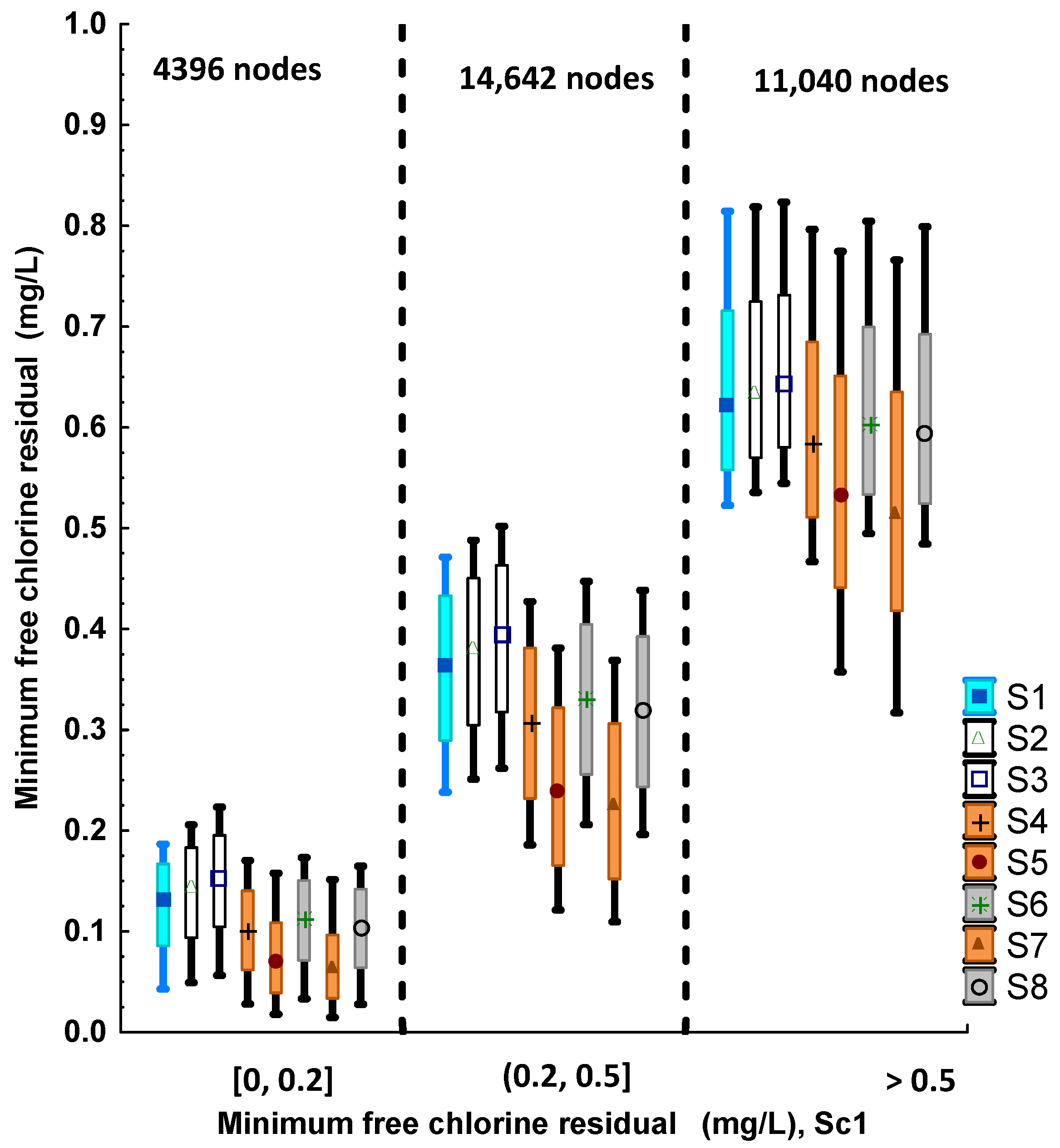
Figure 2 shows the distribution of daily minimum chlorine residuals for Sc1 to Sc8. The nodes were categorized based on their daily minimum chlorine concentration in the reference scenario (Sc1) to better visualize the impact of demand variation scenarios. In Sc1, the minimum chlorine residual was between 0 and 0.2 mg/L for 4396 nodes, with a median of 0.13 mg/L. It should be noted that these are the nodes that are most vulnerable to potential contamination because of their low disinfectant residual concentration. In all the water conservation scenarios (Sc4 to Sc8), 25% of the abovementioned nodes experienced an even lower minimum chlorine residual of less than 0.07 mg/L. For the same group of nodes, the median increased to 0.15 mg/L in Sc3, while it dropped to 0.07 and 0.06 mg/L in Sc5 and Sc7, respectively. A similar trend was observed for the second group of nodes (49% of all nodes), experiencing a minimum Cl2 > 0.2 mg/L during the whole day under the reference scenario. However, a fraction of these nodes experienced a minimum Cl2 < 0.2 mg/L under the studied water conservative scenarios, depending on the severity of the water demand reduction. The percentage of nodes in the second group with a minimum Cl2 < 0.2 mg/L was significantly higher in Sc5 and Sc7 (i.e., >25% of the nodes).
3.3. Impact of Water Demand Variations on Chlorine Reliability
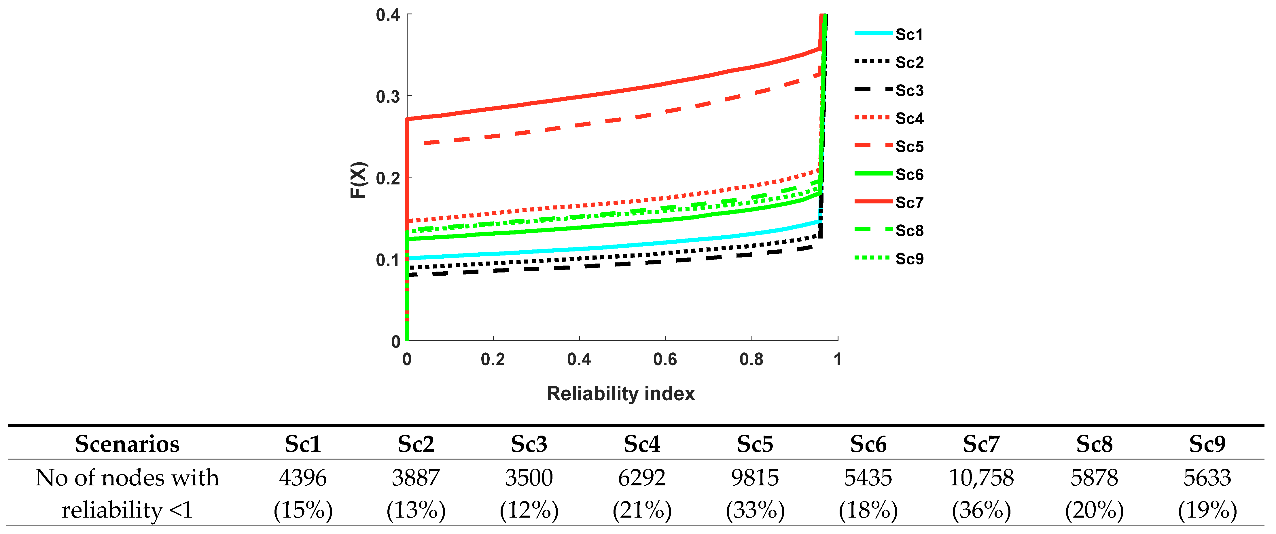
While minimum residual concentration at any time was informative, the chlorine reliability indicator provided more actionable information. Figure 3 is plotted based on the estimated chlorine reliability indicators at each node integrating the duration of low chlorine residuals (<0.2 mg/L), indicative of the severity of the chlorine loss. For the reference scenario (Sc1), a chlorine reliability of less than or equal to 0.9 was observed for about 14% of nodes, while it reached 34% under the most extreme future water conservation scenario. The number of nodes with a chlorine reliability lower than one ranged from 4396 for Sc1 to 10,758 in Sc7.
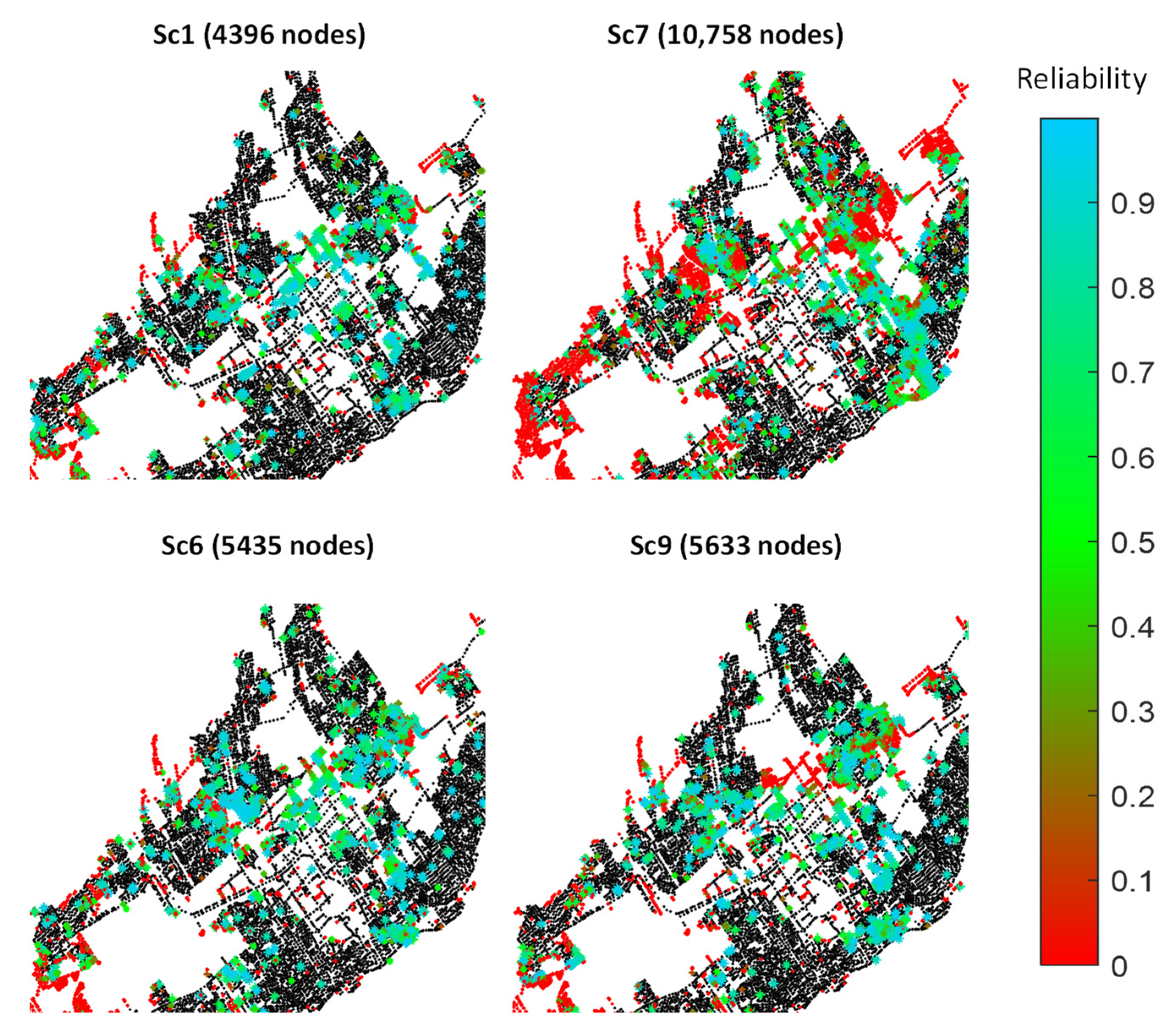
It was also important to consider the spatial distribution of nodal chlorine reliability considering various scenarios of demand reduction intensity (Sc6, Sc7, Sc9) in comparison to the reference scenario (Sc1) (Figure 4). While Sc6 focuses on investigating the effect of reducing residential consumptions, Sc9 aims to investigate the impact of lower I-C-I demand consumptions resulting from extensive lockdown of industrial, commercial, and institutional facilities. Such emergency response shutdowns can result from extreme climate events or a response to a pandemic such as the current COVID-19 pandemic. I-C-I demands were reduced to a minimum in Sc9 from the current scenario (Sc1), while other demand types they remained as in Sc1. Although the global multiplicative factors for Sc6 and Sc9 (0.86 vs. 0.84, Table 1) and the fraction of nodes with a chlorine reliability of less than one (18% vs. 19%, Figure 3) remained almost the same, the spatial distribution of nodal chlorine reliability for these two scenarios was quite different at some areas (Figure 4). The impact of the most severe scenario (47% of global demand and 82% of residential demand reduction) was observed by comparing the geographical distribution of the chlorine reliability indicators in Sc1 and Sc7 (Figure 4).
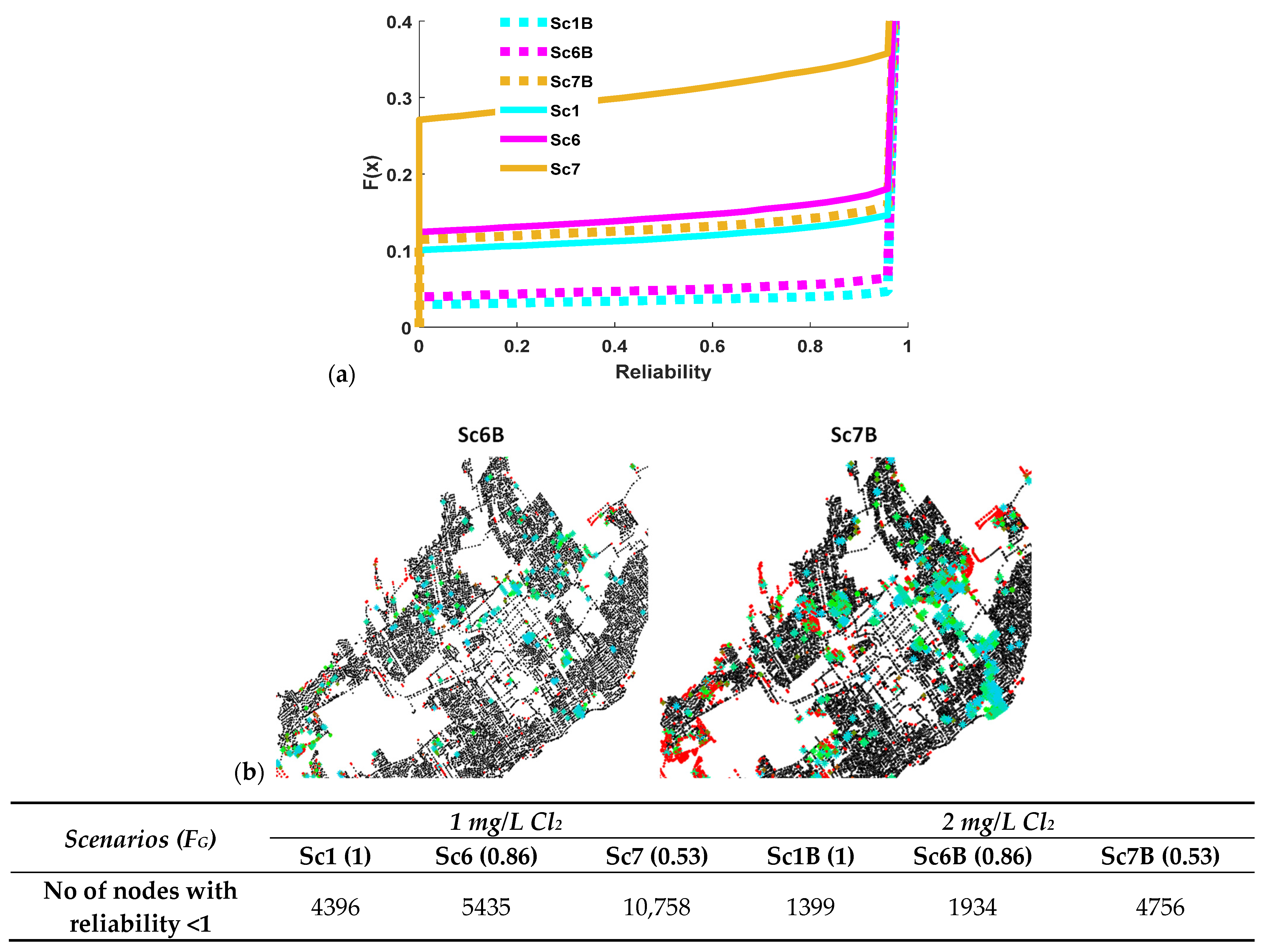
Installing chlorine booster stations at strategic network locations or increasing the outlet disinfectant dose directly at the sources are among commonly used measures to increase disinfectant residuals throughout the network [29]. To test the network robustness to lower demand, the chlorine concentrations at the outlet of each of the three WTPs were increased to 2 mg/L. This allowed for investigating the potential of increasing chlorine dosage at the WTPs to compensate for the performance degradation under water conservation scenarios. Chlorine adjustments were tested for three scenarios (Sc1, Sc6, and Sc7) with different global multiplicative factors (1, 0.86, and 0.53) and are referred to as Sc1B, Sc6B, and Sc7B, respectively. Figure 5a shows that this intervention can remarkably improve the reliability of the network in terms of maintaining target chlorine residuals (here considered ≥0.2 mg/L). Interestingly, chlorine reliability improved so remarkably in the most extreme water conservation scenario (Sc7) after increasing to 2 mg Cl2/L (Sc7B), that the cumulative probability distribution of the reliability was very close to that of the reference scenario. While about 14% of the nodes showed a chlorine reliability of less than or equal to 0.9 under the reference scenario (Sc1), this value slightly increased to 15% under the most extreme future water conservation scenario with increased chlorine dosage at the WTPs (Sc7B), as compared to 34% without any intervention (Sc7). As shown in Figure 5a, even better results were achieved in Sc6B (FG = 0.86, 2 mg/L Cl2) as compared to the reference scenario (Sc1).
3.4. Impact of Lower Water Demand on THMs
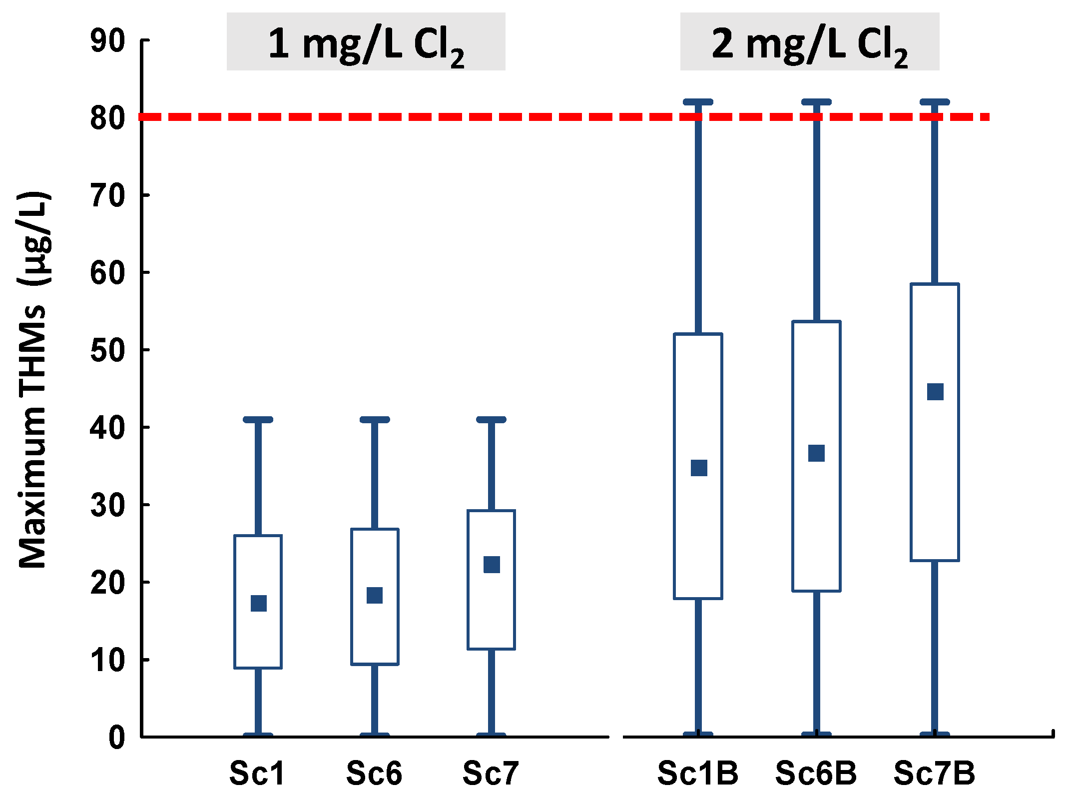
Different parameters such as water age, chlorine dose, pH, and water temperature can contribute to the formation of THMs and other chlorination by-products throughout the network. Therefore, increasing chlorine dosage in order to compensate for future water conservation strategies should be weighed against the risk of increasing THM levels. The distribution of daily maximum modeled THM levels across the network is illustrated for Sc1, Sc6 and Sc7, and with an increased chlorine dosage (Sc1B, Sc6B and Sc7B) (Figure 6). THM concentrations generally increased under water conservation conditions because of increased water age and chlorine consumption. However, resulting THM concentrations remained well below current standards because of the quality of the treated water. Lower demand resulted in slightly higher median THM concentrations (from 17 µg/L in Sc1 to 22 µg/L in Sc7) with 90% ranging from 26 to 29 µg/L. In the case of doubling the chlorine dosage at the WTP outlet, an even more significant increase in THM formation was observed with a maximum value of 82 µg/L. When doubling the chlorine dosage, median concentrations increased from 35 µg/L (Sc1B) to 45 µg/L (Sc7B). These modeled results showed that maintaining a residual of 0.2 mg/L across the system increased concentrations of formed THMs; however, under the studied conditions, it did not lead to noncompliance with acceptable levels set by standards and guidance THMs.
3.5. Impact of Various Water Demand Conditions on Pipe Water Velocity
Water velocity throughout the pipe system was investigated during various demand periods of the year, including average day (ScA), average winter day (ScB), and maximum day (ScC). Table S1 shows that only 15% of the network length with D ≤ 200 mm was designed to experience a daily maximum velocity ≥0.2 m/s during the maximum day, even before implementing any water conservation measures. This value was ≤5% for the actual average day scenario (ScA) and average winter day scenario (ScB).
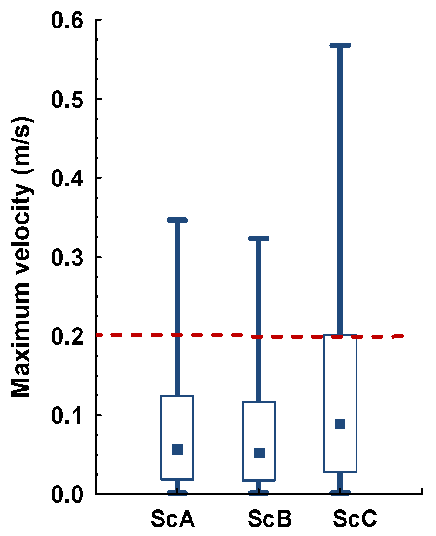
Distributions of maximum velocity in scenarios ScA, ScB, and ScC are illustrated in Figure 7. The median value for all three scenarios was <0.1 m/s, while the 75th percentile increased from about 0.1 m/s in ScB, to 0.2 m/s in ScC (Figure 7). Distributions of maximum daily velocity vs. pipe diameter for the scenarios of average day, average winter day, and maximum day were also investigated (Figure S7). For both groups of pipes (D ≤ 100 mm and 100 < D ≤ 200 mm), the 75th percentile maximum velocity never reached 0.2 m/s, even in the maximum day scenario.
4. Discussion
4.1. Impact of Conservation Demand Scenarios on Water Quality
Various measures aimed at increasing disinfectant residuals, such as chlorine booster stations, disinfectant dose increase at the plant outlet, automated or manual flushing, flowing blowoffs, and other types of demand increase or positioning (e.g., when feasible, connecting a large consumer as the last user on a dead-end pipe) have been described in the literature [29,30].
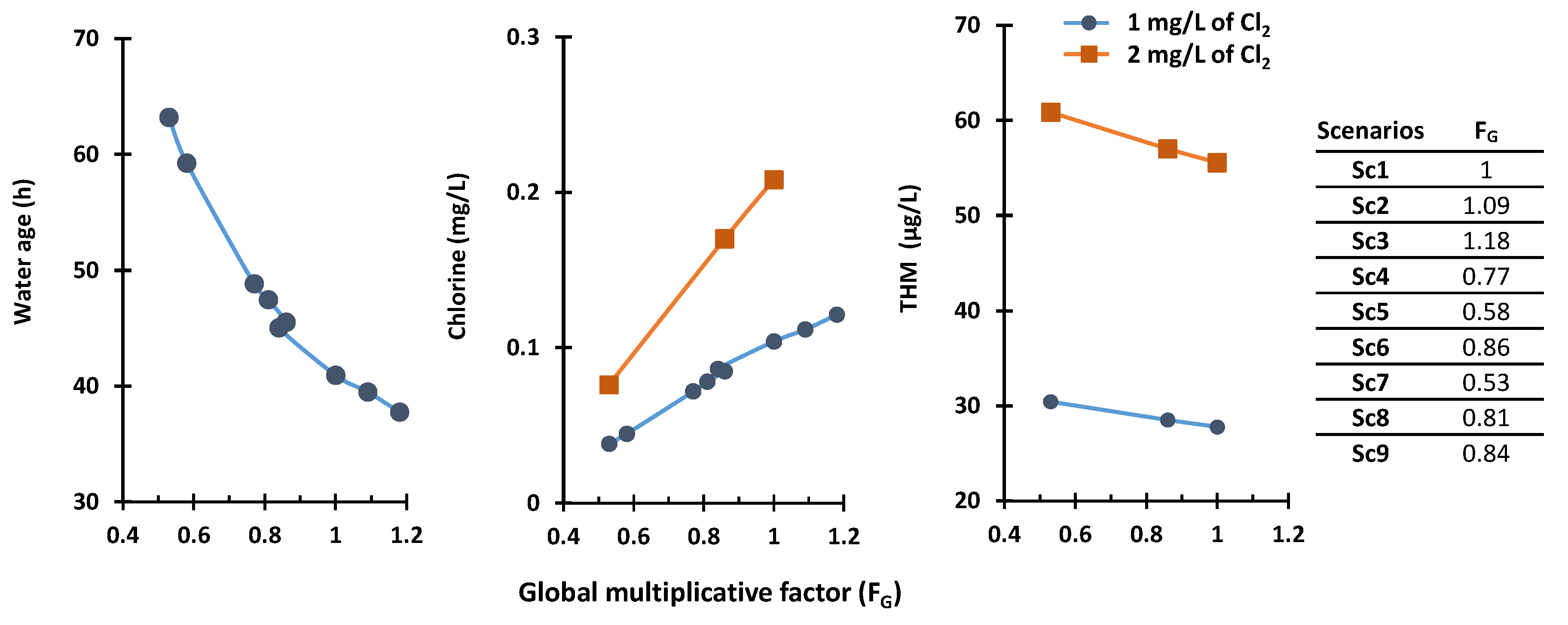
Various water quality parameters including water age, residual free chlorine concentrations, and THM levels were selected to evaluate the water quality performance under eight generated water conservation scenarios with different demand intensities and spatial distributions. Figure 8 summarizes the impact of the severity of water demand changes, represented by a global multiplicative factor, on the values of the water quality parameters. To assist in the discussion, the values plotted were the 95th percentile of nodal maximum water age and THM concentration and the 5th percentile of nodal minimum free chlorine level. The results indicated clearly that water quality generally deteriorated as the total water consumption decreased, and the increased water age resulted in lower chlorine residuals and higher THM levels across the system.
The implications of the chlorine residual losses resulting from varying scenarios depend on the severity of demand reduction. The presence of a residual disinfectant is recommended by some countries, such as the US and the UK [31]. Maintaining measurable chlorine residuals is considered an indispensable measure to prevent microbial regrowth and an important barrier to contamination by ingress water. On the other hand, in most European countries, secondary disinfectants are not applied, reflecting the high level of source protection and treatment and the low vulnerability of DSs to ingress [31]. Maintaining chlorine across a system can increase the formation of toxic disinfection by-products, and taste and odor issues [32]. The efficacy of low chlorine residuals in DSs to inactivate contaminating water has been challenged [33,34] and proof of the ability of disinfectant residuals to prevent waterborne diseases caused by opportunistic pathogens in surface water is lacking [31]. Recent studies across numerous DSs in the US have shown that the prevalence of opportunistic pathogens such as Mycobacterium and Legionella was lower in the presence of a detectable free chlorine residual (>0.1 mg/L) [35]. Some regulations specifically prescribe minimum levels of free chlorine (e.g., detectable, 0.1 or 0.2 mg/L) throughout the network [29] or at a high percentage of sampled locations (95%). For example, based on 40 CFR 141.72, the residual disinfectant concentration in the network “cannot be undetectable in more than 5% of the samples each month” [36].
Figure 8 illustrates the significant challenge if chlorine residuals were to be maintained at all times over a reference value of 0.1 or 0.2 mg/L Cl2 in 95% of the studied network. A reference value of 0.2 mg/L was clearly not achievable in the current operational reference scenario and even less so considering all water conservation scenarios. While only 5% of nodes experienced a chlorine residual of less than 0.1 mg/L during the day in the current operational reference scenario, this value increased to 16% under the most extreme water conservation scenario (Sc7) (Figure S4). A different view of the challenges of meeting minimum residuals across the system was provided by the chlorine reliability indicator. If the disinfectant residual is to be maintained at ≥0.2 mg/L 90% of the time (0.9), reliability will be achieved in 86% (Cl2) of the nodes under the reference scenario and will decrease to 66% (Cl2) of nodes under the most extreme future water conservation scenario. If the level of THMs is to be maintained at ≤80 ug/L, THM reliability of 1 will be achieved at all the nodes in Sc1, Sc6, and Sc7 at 1 mg/L Cl2 (Figure 6).
To almost restore the initial chlorine residual coverage, chlorine dosage at the outlet of the WTPs would need to be increased to a value of 2 mg/L Cl2. Residual maintenance across the system was remarkably improved even for the most extreme water conservation scenario (chlorine reliability achieved at 85% of nodes as compared to 66% of nodes). This showed that it was possible to reconcile water conservation and the maintenance of residual chlorine in the studied network, but at the cost of increased (by a factor of 2) yet compliant THM levels (THM reliability was achieved 90% of the time at almost all the nodes (99.8%)). It can be argued that considering the 95th centile values obtained by modeling (Figure 8) reflected the intent of disinfection by-product regulations that rely on sampling at points with elevated or maximum water age to protect all users from excessive exposure. While the system may remain compliant with the 80 ug/L standard, the exposure to THMs and other disinfection by-products would significantly increase, raising valid concerns over acceptable risk trade-offs.
It is important to consider that chlorine residuals and associated THM values can vary remarkably during the day at some nodes, reflecting network characteristics, demand patterns, and the resulting water age (Figure S5). When setting a minimal residual goal, it is important to acknowledge that some nodes will only reach the desired levels during daily periods of water use. Figure S6 shows significantly lower concentrations of chlorine and increased THMs during low water usage periods at some nodes. These fluctuations showed the impact of sampling timing on monitoring results. The significance of these variations in terms of microbial protection and exposure to undesirable disinfection by-products have yet to be assessed.
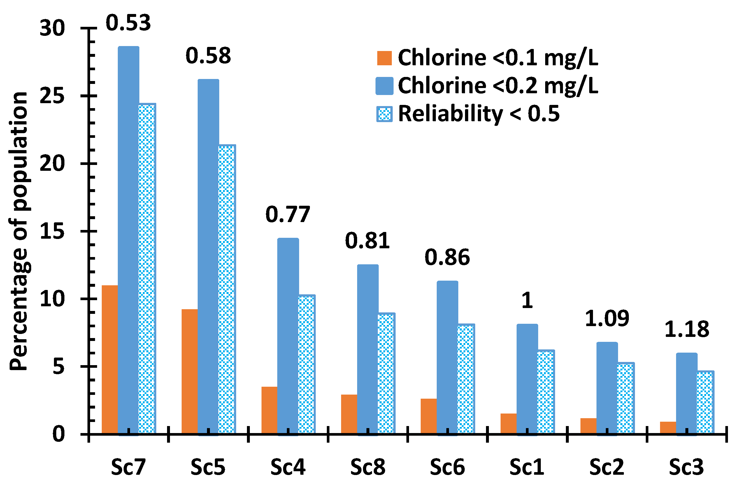
The impact of water conservation scenarios on the number of people supplied with low chlorine residual water at the service connection was also considered (Figure 9). This did not take into account chlorine decay in premise plumbing where water age increases further. The fractions of people supplied with water having a chlorine concentration of <0.2 mg/L (<0.1 mg/L) at any time during the day varied from 6 to 29% (1 to 11%) under different demand scenarios. In Sc6, Sc8 and Sc4, the fraction of the population supplied with water having low chlorine residuals (<0.2 or <0.1 mg/L) progressively increased when compared with the reference scenario (Sc1), while the changes were more substantial in Sc5 and Sc7 (Figure 9).
Finally, nodal reliability indicators in terms of chlorine were used to evaluate the duration over which a population was supplied with a chlorine residual of <0.2 mg/L. Figure 9 shows that the fractions of population exposed to chlorine <0.2 mg/L for more than 12 h during the day (reliability <0.5) varied from 5 to 24%. These results emphasized the need for appropriate operational measures, especially under severe water conservation scenarios, to maintain the performance of DSs. However, it should be considered that despite the intensity of the increase in population percentage, the presence of vulnerable populations (e.g., hospitals and long-term care facilities, daycare centers, etc.) in the low chlorine areas should be considered when managing water conservation programs.
4.2. Remediation Strategies to Improve Water Velocity
Water pipe velocities play an important role in water quality, as red water is a most common cause of customer complaints and has been linked to an increased risk of Legionella [17]. Blokker [37] observed that pipes stay clean (sediment will not accumulate in the pipes) if the maximum velocity reaches 0.2–0.25 m/s once every two days. These self-cleaning recommendations were developed for the tertiary network with smaller pipe diameters (generally <150 mm).
Modeled conditions in the DS were highly favorable to deposition even before implementing any water conservation: 95% of the length of the network with D ≤ 200 mm experienced Vmax < 0.2 m/s in the reference scenario. Our observations were in line with previous reports regarding self-cleaning capacity for conventional layouts (i.e., 6%) [23]. Gibson, et al. [15] also reported low velocities (median = 0.02 m/s) based on North American systems design (fire flow requirements of 3800 L/min and D ≥ 150 mm) when applying an optimization algorithm to maximize the number of pipes with a velocity of >0.1 m/s. However, it should be considered that the self-cleaning reference value of 0.2 m/s was developed in the tertiary network with smaller pipes and without any residual disinfectant. This value may not be applicable to the studied network with larger diameter pipes (D ≤ 200 mm) and in the presence of free chlorine residuals. Existing chlorine residuals can limit biofilm-associated risks such as discoloration [38]. In our network, only 2% of the pipe length had a diameter of 100 mm or smaller, while 67% of pipe length consisted of 200 mm or smaller diameter pipes. Accumulation of loose deposits and corrosion by-products in areas with unlined cast iron piping was addressed by unidirectional flushing on a yearly basis in the studied network.
The very low velocities observed in the studied DS reflected the high fire flows that are recommended by AWWA and insurance companies in North America. In North America, the standard criteria for minimum pipe diameters are 150 mm for loops and 200 mm for dead ends [39]. Revisiting the minimum pipe diameter of 150 mm, redundant loops and high nominal fire flows would bring benefits in terms of capital costs and water quality [15]. Also, employing smaller diameter pipes would result in reduced capital costs, water ages, bacterial growth, and sediment deposition [40,41]. The low water velocities in most of the pipes in the studied network (Figure 7), even without implementing any water conservation program, stressed the need to review fire flow requirements and sources to ensure water quality when designing or extending a drinking water distribution network.
Flushing is widely used as a response to low velocities. Strategies designed to remove deposits, limit red water complaints, or respond to a contamination event have been proposed [42,43]. Automatic drain valves are another alternative option to compensate for changes in water age.
As North American networks are commonly overdesigned, flushing programs will need to be adjusted to compensate the loss of velocity resulting from the implementation of conservation scenarios. As the need for flushing is likely to increase, the trade-offs between water conservation and wasted water during flushing will need to be considered. However, further research is required to determine if an enhanced efficient flushing program would be feasible and could counteract the changes in water age and low velocities.
In fact, a trade-off between water conservation and water quality is necessary in order to maintain the performance and reliability of a water network. All water issues (residual maintenance, disinfection by-products, velocity, taste, and odor, etc.) should be considered simultaneously. Although regulatory attention is directed to the maintenance of a chlorine residual across the system (e.g., by boosting chlorine injection at the WTP outlet or at strategic network locations), this measure does not solve critical issues such as red water events and discoloration or the prevention of Legionella. The costs and benefits of corrective actions made necessary by water conservation, such as flushing or increasing residuals, should also be weighed in terms of public health outcomes.
4.3. Limitations and Future Research
The future water demand scenarios considered were mainly specified based on the adoption of more efficient fixtures and on changes in water consumption behavior, while the effects of population variation and climate change were not taken into account. Population growth and densification of municipalities could, to some extent, compensate future water conservation strategies. In future investigations, more specific network data regarding different factors that can affect outdoor usage, such as house age, irrigation systems, drought restrictions and weather conditions, can be incorporated to enhance future water demand scenarios. The presented approach can be easily tailored to different systems considering their local constraints in reducing different types of demand.
Our observations are valid under the conditions studied in this article. Different reaction rates for bulk and wall chlorine decay and/or the formation of THMs, network characteristics, or temperature variations can affect the results. Future research can investigate the sensitivity of our results to different water quality parameters. It should be considered that the presented approach has no limitation on use other than the availability of the input data. It should also be considered that disregarding dispersion transport mechanisms and spatial demand aggregation can result in overestimation of predicted chlorine concentrations, especially at the dead-end branches, as demonstrated by Abokifa, et al. [27]. Other uncertainties affecting water quality include complete mixing at nodes and plug flow in the model. Also, as demonstrated by Blokker, et al. [44], a hydraulic model with stochastic diurnal patterns can lead to different residual chlorine levels, as compared with considering one specific demand pattern for each user type.
5. Conclusions
In order to assess the impact of various water demand management strategies on the hydraulic and water quality performance of a full-scale DS, nine conceptual water demand scenarios were examined, in which the residential and/or nonresidential consumptions were varied to different extents. The potential impact on water quality was then assessed by analyzing the distribution of water age, the impact on pipe velocity, and the ability to maintain a minimum of 0.2 mg/L free chlorine (reliability index) while meeting the current maximum contaminant level of 80 ug/L THM.
Key findings include:
- Water quality generally gets poorer (i.e., higher water age and THMs and lower free chlorine residuals) under the studied water conservation scenarios as compared to the reference scenario. Nodal water age values increase more for nodes serving smaller diameter pipes, where maintaining water quality is a greater challenge.
- The reliability of maintaining a free chlorine residual was less than or equal to 0.9 for about 14% of the nodes throughout the network under the reference scenario and increased to 34% of the nodes under the most extreme future water conservation scenario. The loss of chlorine reliability across the system raises significant water quality management challenges if regulations require the maintenance of chlorine residuals across the network.
- Increasing chlorine at the outlet of the plant from 1 to 2 mg/L, an easily implemented adjustment, dramatically improves the network reliability in terms of chlorine residual (≥0.2 mg/L). Even in the extreme future water conservation scenario, residual coverage was recovered almost to levels found in the reference scenario. However, this reliability came at the cost of increased yet compliant THM formation, especially in the low demand scenarios, raising the challenge of managing competing water quality goals.
- The spatial distribution of chlorine reliability can assist in determining the areas requiring operational measures such as flushing or optimizing chlorine booster locations under future water conservation programs.
- Self-cleaning velocity is a key factor to controlling turbidity and red-water-related complaints. Any water conservation scenario considered will generally lower critical velocities that may require additional remedial strategies, especially in legacy overdesigned DSs. As red water has recently been linked to an increased risk of Legionella, lower demands in distributions systems will also increase the need for optimal corrosion control.
- For operational measures counteracting demand reduction to be optimal, water quality, network characteristics, total water saving amounts, and the additional burden to operators should be taken into consideration.
- To improve this assessment, more representative future water demand scenarios can be defined by including the effects of population variation and climate change. Other factors such as gradual adoption of water conservation programs, consumers’ behavioral variability, and the impact of different water quality parameters can be considered in further studies.
- These results revealed that in order to provide a framework for water demand management programs and to implement efficient operational measures under water conservation conditions, we should take into consideration not only the total water saving amounts, but also the spatial changes of the anticipated demand reduction.
Supplementary Materials
The following are available online at https://www.mdpi.com/article/10.3390/w13182579/s1, Figure S1: Daily demand patterns, Figure S2: nodal pressure and nodal water loss, Figure S3: Distribution of nodal water age, Figure S4: Number of nodes for various ranges of minimum chlorine residuals, Figure S5: Distribution of chlorine residuals and THMs nodal differences between maximum and minimum values during the day, Figure S6: Variations of chlorine residuals and associated THM values during the day, Figure S7: Maximum velocity vs. pipe diameter, Table S1: Fraction of pipe length with self-cleaning capacity.
Author Contributions
Conceptualization, F.H., M.P. and G.E.; Investigation, methodology and formal analysis, F.H. and M.P.; Software and writing—original draft, F.H.; Writing—review and editing, M.P. and G.E. All authors have read and agreed to the published version of the manuscript.
Funding
This research was funded by the NSERC Industrial Chair on Drinking Water at Polytechnique Montréal.
Institutional Review Board Statement
Not applicable.
Data Availability Statement
Some or all data used/generated during the study are available from the corresponding author by request.
Acknowledgments
The authors would like to thank the participating utility that provided information on the network model and Bentley Systems for providing academic access, with unlimited pipes version. The NSERC Industrial Chair on Drinking Water at Polytechnique Montréal funded this research.
Conflicts of Interest
The authors declare no conflict of interest.
References
- Mayer, P.W. Water Research Foundation study documents water conservation potential and more efficiency in households. J. AWWA 2016, 108, 31–40. [Google Scholar] [CrossRef]
- Parker, J.M.; Wilby, R.L. Quantifying household water demand: A review of theory and practice in the UK. Water Resour. Manag. 2013, 27, 981–1011. [Google Scholar] [CrossRef] [Green Version]
- Gurung, T.R.; Stewart, R.A.; Sharma, A.K.; Beal, C.D. Smart meters for enhanced water supply network modelling and infrastructure planning. Resour. Conserv. Recycl. 2014, 90, 34–50. [Google Scholar] [CrossRef] [Green Version]
- Arbués, F.; García-Valiñas, M.Á.; Martínez-Espiñeira, R. Estimation of residential water demand: A state-of-the-art review. J. Socio-Econ. 2003, 32, 81–102. [Google Scholar] [CrossRef]
- Pickard, B.R.; Nash, M.; Baynes, J.; Mehaffey, M. Planning for community resilience to future United States domestic water demand. Landsc. Urban Plan. 2017, 158, 75–86. [Google Scholar] [CrossRef] [PubMed] [Green Version]
- Pidou, M.; Memon, F.A.; Stephenson, T.; Jefferson, B.; Jeffrey, P. Greywater recycling: Treatment options and applications. Proc. Inst. Civ. Eng. Eng. Sustain. 2007, 160, 119–131. [Google Scholar] [CrossRef] [Green Version]
- Byrne, J.; Dallas, S.; Anda, M.; Ho, G. Quantifying the benefits of residential greywater reuse. Water 2020, 12, 2310. [Google Scholar] [CrossRef]
- Sitzenfrei, R.; Zischg, J.; Sitzmann, M.; Bach, P.M. Impact of hybridwater supply on the centralised water system. Water 2017, 9, 855. [Google Scholar] [CrossRef] [Green Version]
- Gregg, T.T.; Strub, D.; Gross, E. Water efficiency in Austin, Texas, 1983–2005: An historical perspective. J. AWWA 2007, 99, 76–86. [Google Scholar] [CrossRef]
- Water Research Foundation (WRF). Residential End Uses of Water; Version 2; WRF: Denver, CO, USA, 2016; p. 363. [Google Scholar]
- Mayer, P.W.; DeOreo, W.B.; Opitz, E.M.; Kiefer, J.C.; Davis, W.Y.; Dziegielewski, B.; Nelson, J.O. Residential End Uses of Water (Executive Summary); American Water Works Association Research Foundation and Aquacraft, Inc.: Denver, CO, USA, 1999. [Google Scholar]
- Mayer, P.W.; DeOreo, W.B.; Lewis, D.M. Seattle Home Water Conservation Study. The Impacts of High Efficiency Plumbing Fixture Retrofits in Single-Family Homes; Submitted to Seattle Public Utilities and The United States Environmental Protection Agency; Aquacraft, Inc., Water Engineering and Management: Boulder, CO, USA, 2000; p. 10. [Google Scholar]
- Gheisi, A.; Forsyth, M.; Naser, G. Water distribution systems reliability: A review of research literature. J. Water Resour. Plan. Manag. 2016, 142, 04016047. [Google Scholar] [CrossRef]
- Huang, J.; McBean, E.; James, W. A review of reliability analysis for water quality in water distribution systems. J. Water Manag. Model. 2005, 7, 107–130. [Google Scholar] [CrossRef] [Green Version]
- Gibson, J.; Karney, B.; Guo, Y. Water quality and fire protection trade-offs in water distribution networks. J. Am. Water Work. Assoc. 2019, 111, 44–52. [Google Scholar] [CrossRef]
- Vreeburg, J.H.G.; Boxall, J.B. Discolouration in potable water distribution systems: A review. Water Res. 2007, 41, 519–529. [Google Scholar] [CrossRef] [PubMed]
- Rhoads, W.J.; Garner, E.; Ji, P.; Zhu, N.; Parks, J.; Schwake, D.O.; Pruden, A.; Edwards, M.A. Distribution system operational deficiencies coincide with reported legionnaires’ disease clusters in Flint, Michigan. Environ. Sci. Technol. 2017, 51, 11986–11995. [Google Scholar] [CrossRef]
- Fu, G.; Kapelan, Z.; Kasprzyk Joseph, R.; Reed, P. Optimal design of water distribution systems using many-objective visual analytics. J. Water Resour. Plan. Manag. 2013, 139, 624–633. [Google Scholar] [CrossRef] [Green Version]
- Kanta, L.; Zechman, E.; Brumbelow, K. Multiobjective evolutionary computation approach for redesigning water distribution systems to provide fire flows. J. Water Resour. Plan. Manag. 2012, 138, 144–152. [Google Scholar] [CrossRef]
- Gupta, R.; Dhapade, S.; Ganguly, S.; Bhave, P.R. Water quality based reliability analysis for water distribution networks. ISH J. Hydraul. Eng. 2012, 18, 80–89. [Google Scholar] [CrossRef]
- Blokker, E.; Vreeburg, J.; Schaap, P.; van Dijk, J. The self-cleaning velocity in practice. In Proceedings of the Water Distribution System Analysis Conference, Tucson, AZ, USA, 12–15 September 2010; p. 13. [Google Scholar]
- van Dijk, J.C.; Horst, P.; Blokker, E.J.M.; Vreeburg, J.H.G. Velocity-based self-cleaning residential drinking water distribution systems. Water Supply 2009, 9, 635–641. [Google Scholar]
- Agudelo-Vera, C.; Blokker, M.; Vreeburg, J.; Vogelaar, H.; Hillegers, S.; van der Hoek, J.P. Testing the robustness of two water distribution system layouts under changing drinking water demand. J. Water Resour. Plan. Manag. 2016, 142, 05016003. [Google Scholar] [CrossRef] [Green Version]
- Basupi, I.; Kapelan, Z. Flexible water distribution system design under future demand uncertainty. J. Water Resour. Plan. Manag. 2015, 141, 04014067. [Google Scholar] [CrossRef]
- Tsegaye, S.; Gallagher, K.C.; Missimer, T.M. Coping with future change: Optimal design of flexible water distribution systems. Sustain. Cities Soc. 2020, 61, 102306. [Google Scholar] [CrossRef]
- Zhuang, J.; Sela, L. Impact of emerging water savings scenarios on performance of urban water networks. J. Water Resour. Plan. Manag. 2020, 146, 04019063. [Google Scholar] [CrossRef]
- Abokifa, A.A.; Xing, L.; Sela, L. Investigating the impacts of water conservation on water quality in distribution networks using an advection-dispersion transport model. Water 2020, 12, 1033. [Google Scholar] [CrossRef] [Green Version]
- United States Environmental Protection Agency (USEPA). EPA Drinking Water Guidance on Disinfection by-Products. Advice Note No. 4. Version 2. Disinfection by-Products in Drinking Water; USEPA: Washington, DC, USA, 2012; p. 27. [Google Scholar]
- Walski, T. Raising the bar on disinfectant residuals. World Water 2019, 35, 2. [Google Scholar]
- Avvedimento, S.; Todeschini, S.; Giudicianni, C.; Di Nardo, A.; Walski, T.; Creaco, E. Modulating nodal outflows to guarantee sufficient disinfectant residuals in water distribution networks. J. Water Resour. Plan. Manag. 2020, 146, 04020066. [Google Scholar] [CrossRef]
- Rosario-Ortiz, F.; Rose, J.; Speight, V.; von Gunten, U.; Schnoor, J. How do you like your tap water? Science 2016, 351, 912–914. [Google Scholar] [CrossRef]
- Hrudey, S.E. Chlorination disinfection by-products, public health risk tradeoffs and me. Water Res. 2009, 43, 2057–2092. [Google Scholar] [CrossRef] [PubMed]
- Payment, P. Poor efficacy of residual chlorine disinfectant in drinking water to inactivate waterborne pathogens in distribution systems. Can. J. Microbiol. 1999, 45, 709–715. [Google Scholar] [CrossRef] [PubMed]
- Hatam, F.; Besner, M.-C.; Ebacher, G.; Prévost, M. Limitations of E. coli monitoring for confirmation of contamination in distribution systems due to intrusion under low pressure conditions in the presence of disinfectants. J. Water Resour. Plan. Manag. 2020, 146, 04020056. [Google Scholar] [CrossRef]
- Donohue, M.J.; Vesper, S.; Mistry, J.; Donohue, J.M. Impact of chlorine and chloramine on the detection and quantification of Legionella pneumophila and Mycobacterium species. Appl. Environ. Microbiol. 2019, 85, e01942-19. [Google Scholar] [CrossRef] [PubMed] [Green Version]
- Code of Federal Regulations (CFR). National Primary Drinking Water Regulations, Subpart H—Filtration and Disinfection, Disinfection; 40 CFR 141.72; U.S. Government: Washington, DC, USA, 2010; pp. 456–458. [Google Scholar]
- Blokker, E.J.M. Stochastic Water Demand Modelling for a Better Understanding of Hydraulics in Water Distribution Networks; Water Management Academic Press: Delft, The Netherlands, 2010; p. 218. [Google Scholar]
- Fish, K.E.; Reeves-McLaren, N.; Husband, S.; Boxall, J. Unchartered waters: The unintended impacts of residual chlorine on water quality and biofilms. NPJ Biofilms Microbiomes 2020, 6, 34. [Google Scholar] [CrossRef] [PubMed]
- American Water Works Association (AWWA). M31 Distribution System Requirements for Fire Protection, 4th ed.; American Water Works Association (AWWA): Denver, CO, USA, 2008. [Google Scholar]
- Myburgh, H.M.; Jacobs, H.E. Water for firefighting in five South African towns. Water SA 2014, 40, 11–18. [Google Scholar] [CrossRef]
- Gibson, J.; Karney, B.; Guo, Y. Effects of relaxed minimum pipe diameters on fire flow, cost, and water quality indicators in drinking water distribution networks. J. Water Resour. Plan. Manag. 2020, 146, 04020059. [Google Scholar] [CrossRef]
- Carrière, A.; Gauthier, V.; Desjardins, R.; Barbeau, B. Evaluation of loose deposits in distribution systems through unidirectional flushing. J. Am. Water Work. Assoc. 2005, 97, 82–92. [Google Scholar] [CrossRef]
- Haxton, T.B.; Walski, T.M. Modeling a hydraulic response to a contamination event. In Proceedings of the World Environmental and Water Resources Congress 2009, Kansas City, MO, USA, 17–21 May 2009; pp. 575–583. [Google Scholar]
- Blokker, M.; Vreeburg, J.; Speight, V. Residual chlorine in the extremities of the drinking water distribution system: The influence of stochastic water demands. Procedia Eng. 2014, 70, 172–180. [Google Scholar] [CrossRef] [Green Version]
Figure 1.
(a) Distribution of nodal differences in daily maximum water age from Sc2 to Sc8 and the current scenario (Sc1); Median; Box: 25–75%; Whisker: 10–90%; and (b) Median of maximum water age differences (from Figure 1a) vs. the associated global multiplicative factor (FG).
Figure 1.
(a) Distribution of nodal differences in daily maximum water age from Sc2 to Sc8 and the current scenario (Sc1); Median; Box: 25–75%; Whisker: 10–90%; and (b) Median of maximum water age differences (from Figure 1a) vs. the associated global multiplicative factor (FG).

Figure 2.
Distribution of nodal minimum chlorine residuals in Sc1 to Sc8, for all nodes in the network that were categorized based on their daily minimum chlorine concentration under the current scenario (Sc1); Median; Box: 25–75%; Whisker: 10–90%.
Figure 2.
Distribution of nodal minimum chlorine residuals in Sc1 to Sc8, for all nodes in the network that were categorized based on their daily minimum chlorine concentration under the current scenario (Sc1); Median; Box: 25–75%; Whisker: 10–90%.

Figure 3.
Probability that the chlorine reliability indicator will be ≤x for different water conservation scenarios considering all nodes, Y-axis is cut at 0.4 for better visualization. The number and fraction of nodes with a chlorine reliability of less than one are included in the table.
Figure 3.
Probability that the chlorine reliability indicator will be ≤x for different water conservation scenarios considering all nodes, Y-axis is cut at 0.4 for better visualization. The number and fraction of nodes with a chlorine reliability of less than one are included in the table.

Figure 4.
Spatial distribution of nodal chlorine reliability with a value of less than one in Sc1, Sc6, Sc7, and Sc9. Reliability values are represented by both color and size (a function of its value).
Figure 4.
Spatial distribution of nodal chlorine reliability with a value of less than one in Sc1, Sc6, Sc7, and Sc9. Reliability values are represented by both color and size (a function of its value).

Figure 5.
(a) Probability that the chlorine reliability will be ≤x for different water conservation scenarios considering all nodes, Y-axis is cut at 0.4 for better visualization. (b) Spatial distribution of nodal chlorine reliabilities of less than one in Sc6B and Sc7B (same color legend as in Figure 4). The number of nodes with a chlorine reliability <1 is indicated in the table.

Figure 6.
Distribution of maximum THM levels during a whole day period for all nodes in Sc1, Sc6, and Sc7 at 1 and 2 mg/L Cl2 at the WTPs. Median; Box: 10–90%; Whisker: min-max. Red line: maximum acceptable level of THMs (80 μg/L) (USEPA, 2012).
Figure 6.
Distribution of maximum THM levels during a whole day period for all nodes in Sc1, Sc6, and Sc7 at 1 and 2 mg/L Cl2 at the WTPs. Median; Box: 10–90%; Whisker: min-max. Red line: maximum acceptable level of THMs (80 μg/L) (USEPA, 2012).

Figure 7.
Maximum velocity distribution for scenarios of average day (ScA), average winter day (ScB), and maximum day (ScC) (Table 2). Median; Box: 25–75%; Whisker: 5–95%.
Figure 7.
Maximum velocity distribution for scenarios of average day (ScA), average winter day (ScB), and maximum day (ScC) (Table 2). Median; Box: 25–75%; Whisker: 5–95%.

Figure 8.
Water quality variations (water age, chlorine residuals, THMs) in different scenarios based on the global demand multiplicative factor corresponding to each scenario, for 1 and 2 mg/L free chlorine residuals at the WTPs’ outlet. The 95th percentile of nodal maximum water age and THM concentration and the 5th percentile of nodal minimum free chlorine level of all nodes.

Figure 9.
Fraction of total population supplied with water having a daily minimum chlorine level of <0.2 and <0.1 mg/L and a chlorine reliability of <0.5, using 0.2 mg/L as the threshold. The global multiplicative factor (FG) for each scenario is indicated above each column.
Figure 9.
Fraction of total population supplied with water having a daily minimum chlorine level of <0.2 and <0.1 mg/L and a chlorine reliability of <0.5, using 0.2 mg/L as the threshold. The global multiplicative factor (FG) for each scenario is indicated above each column.


Table 1.
Residential demand in liters per capita per day (LCD), and the implemented multiplicative factors for different user types: residential, industrial–commercial–institutional (I-C-I), and municipal for nine water demand scenarios. The global multiplicative factor (FG) is the ratio of the scenario total demand to the total network demand of Sc1.
| Scenarios | Residential demand (LCD) | Description/Reference for Residential Demand | Multiplicative Factor | |||||
|---|---|---|---|---|---|---|---|---|
| Indoor | Outdoor | Total | Residential | I-C-I | Municipal | FG | ||
| Sc1 (Current) | 259 | Average day of 2015 for the studied network | 1 | 1 | 1 | 1 | ||
| Sc2 | 222 | 82 | 304 | Indoor use: based on nine utilities (737 homes) surveys (REU2016) (WRF, 2016) and outdoor use: 27% of the total residential based on 23,749 single-family homes surveys (WRF, 2016) | 1.17 | 1 | 1 | 1.09 |
| Sc3 (Past) | 347 | Average day of 2005 for the studied network | 1.34 | 1 | 1 | 1.18 | ||
| Sc4 (Future) | 119 | 23 | 142 | Netherlands’ actual average daily drinking water demand (Agudelo-Vera et al., 2016) | 0.55 | 1 | 1 | 0.77 |
| Sc5 (Future) | 47 | 0 | 47 | Netherlands’ most conservative scenario (Agudelo-Vera et al., 2016) | 0.18 | 1 | 1 | 0.58 |
| Sc6 (Future) | 139 | 51 | 190 | Indoor use: EPA’s WaterSense New Home Specifications, and outdoor use: 27% of the total residential (WRF, 2016) | 0.73 | 1 | 1 | 0.86 |
| Sc7 (Future) | 47 | 0 | 47 | Netherlands most conservative scenario (Agudelo-Vera et al., 2016) (Same as Sc5) | 0.18 | 0.8 | 0.8 | 0.53 |
| Sc8 (Future) | 139 | 51 | 190 | Indoor use: EPA’s WaterSense New Home Specifications, and outdoor use: 27% of the total residential (WRF, 2016) (Same as Sc6) | 0.73 | 0.8 | 0.8 | 0.81 |
| Sc9 (Lockdown) | 259 | Average day of 2015 for the studied network (Same as Sc1) | 1 | 0 | 1 | 0.84 | ||
Table 2.
Scenarios for investigating the self-cleaning capacity.
| Scenarios | Period | Total Flow Rate m3/day | FG | FR |
|---|---|---|---|---|
| ScA (Same as Sc1, Table 1) | Average day, 2015 | 210,364 | 1 | 1 |
| ScB | Average winter day November to March, 2014 | 199,000 | 0.95 | 0.90 |
| ScC | Maximum day, 2015 | 315,550 | 1.50 | 1.97 |
Publisher’s Note: MDPI stays neutral with regard to jurisdictional claims in published maps and institutional affiliations. |
© 2021 by the authors. Licensee MDPI, Basel, Switzerland. This article is an open access article distributed under the terms and conditions of the Creative Commons Attribution (CC BY) license (https://creativecommons.org/licenses/by/4.0/).
Share and Cite
MDPI and ACS Style
Hatam, F.; Ebacher, G.; Prévost, M. Stringency of Water Conservation Determines Drinking Water Quality Trade-Offs: Lessons Learned from a Full-Scale Water Distribution System. Water 2021, 13, 2579. https://doi.org/10.3390/w13182579
AMA Style
Hatam F, Ebacher G, Prévost M. Stringency of Water Conservation Determines Drinking Water Quality Trade-Offs: Lessons Learned from a Full-Scale Water Distribution System. Water. 2021; 13(18):2579. https://doi.org/10.3390/w13182579
Chicago/Turabian StyleHatam, Fatemeh, Gabrielle Ebacher, and Michèle Prévost. 2021. "Stringency of Water Conservation Determines Drinking Water Quality Trade-Offs: Lessons Learned from a Full-Scale Water Distribution System" Water 13, no. 18: 2579. https://doi.org/10.3390/w13182579
Note that from the first issue of 2016, this journal uses article numbers instead of page numbers. See further details here.