
Development of a Numerical Multi-Layered Groundwater Model to Simulate Inter-Aquifer Water Exchange in Shelby County, Tennessee

 ,
,
Abstract
:1. Introduction
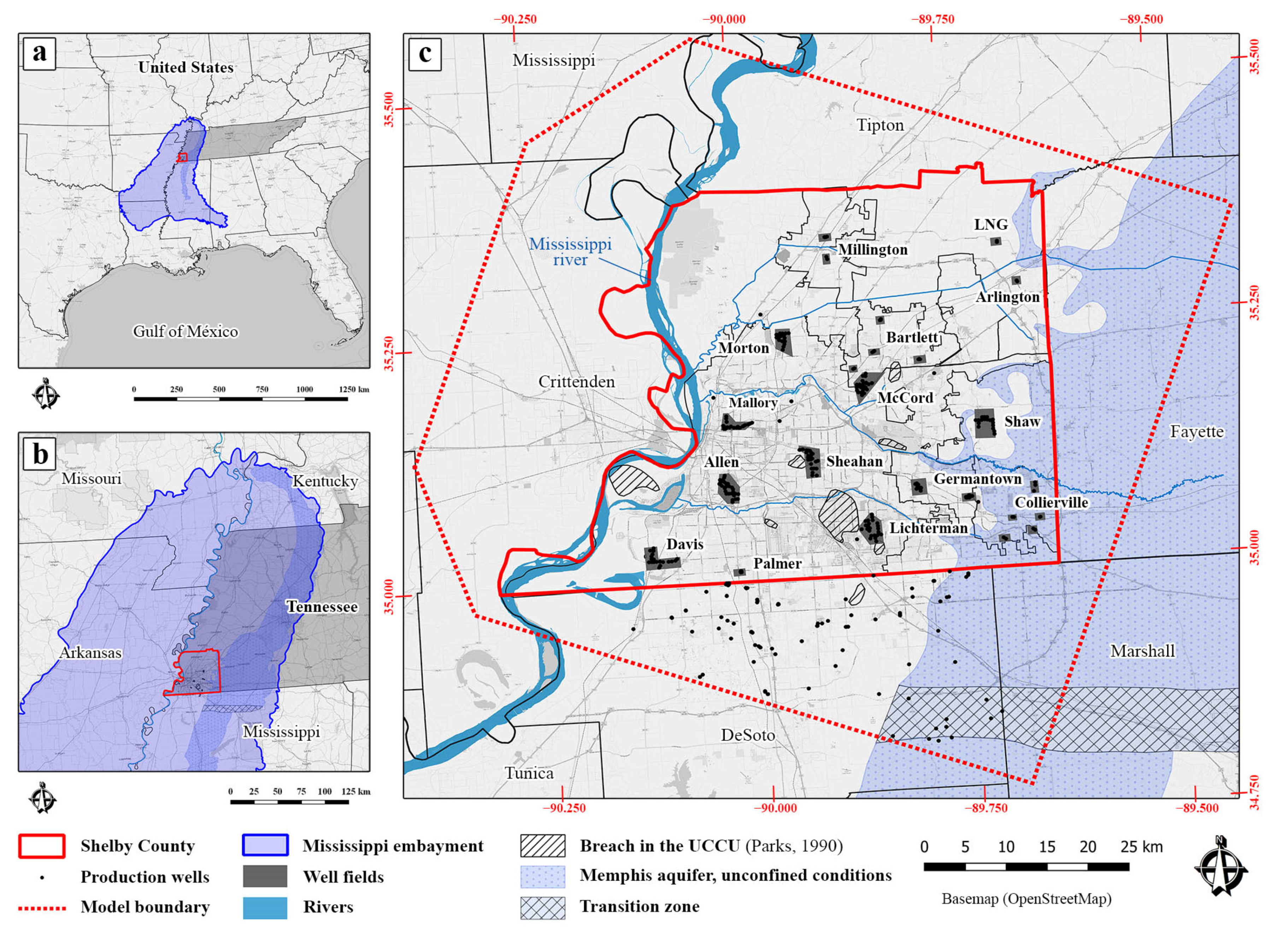
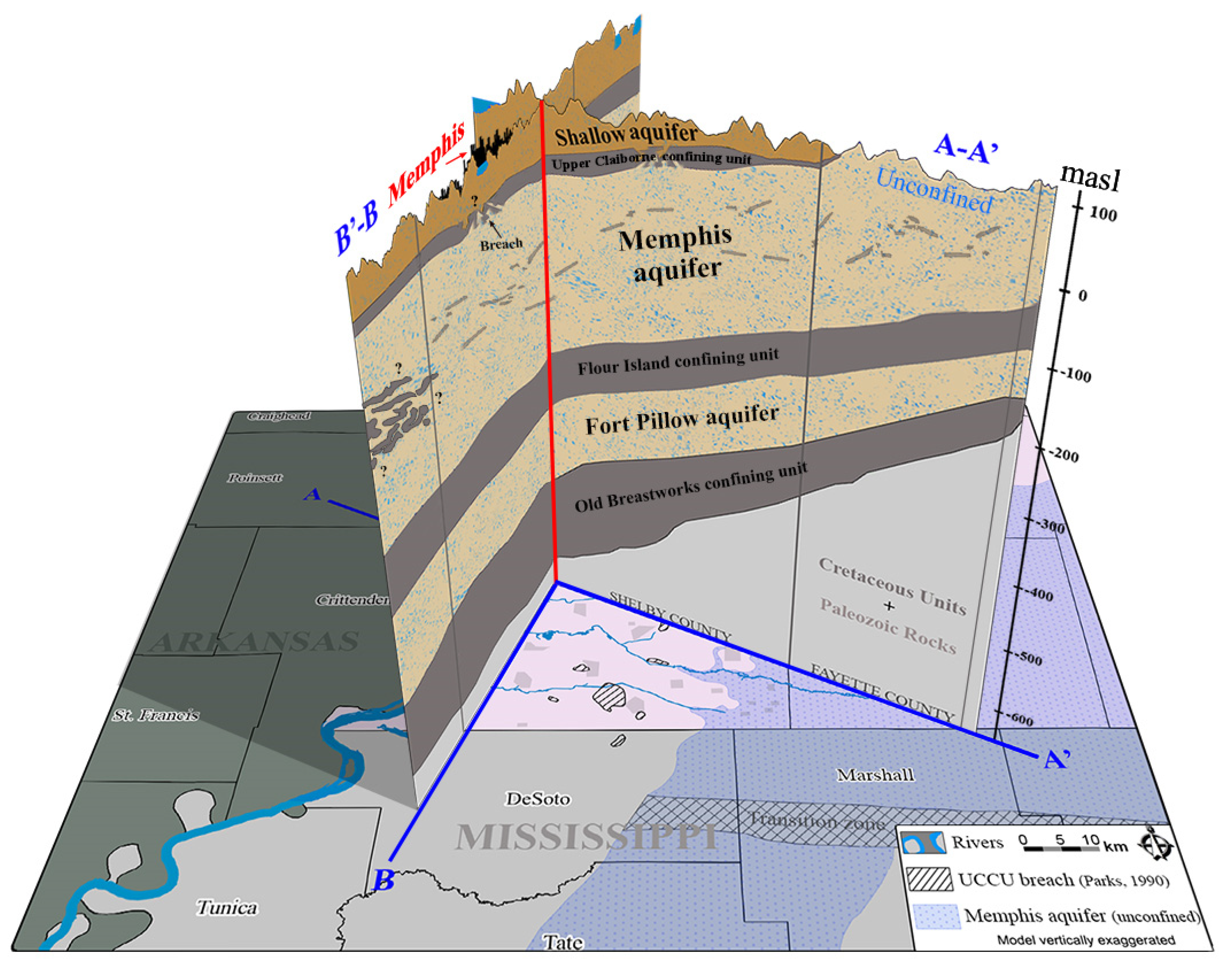
Hydrogeologic Units
2. Materials and Methods
2.1. Conceptual Model
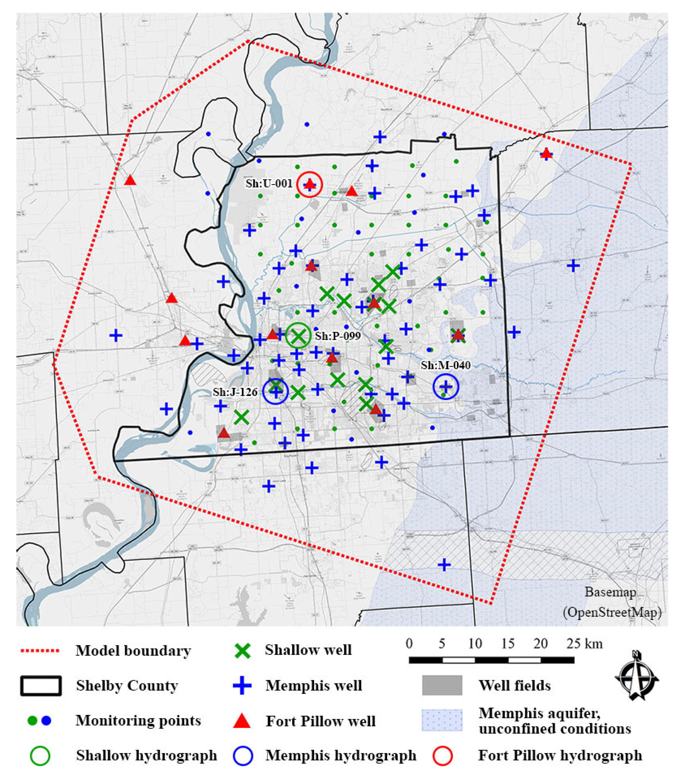
2.1.1. Boundary Conditions
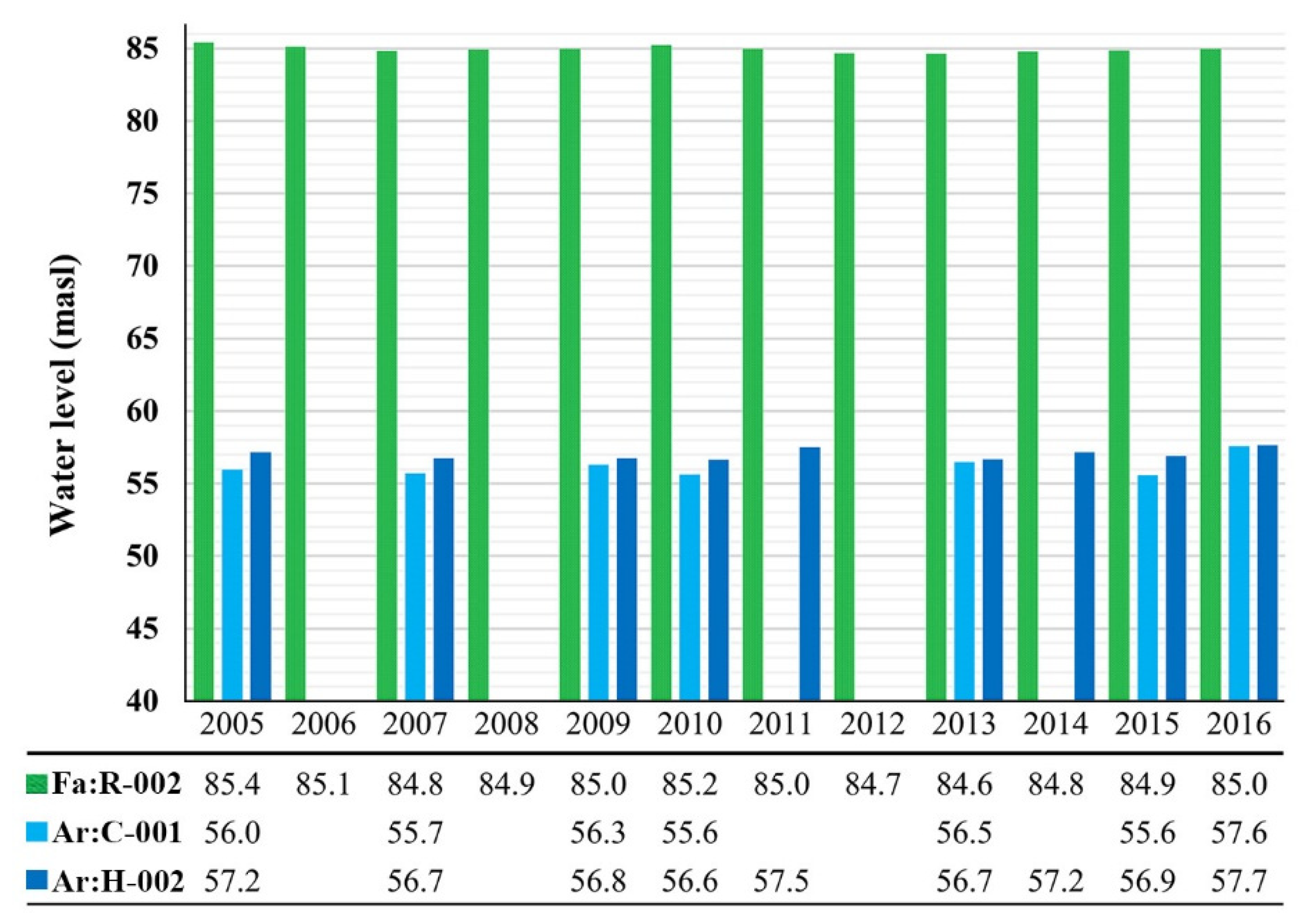
2.1.2. Initial Conditions
2.1.3. Hydraulic Properties and Recharge
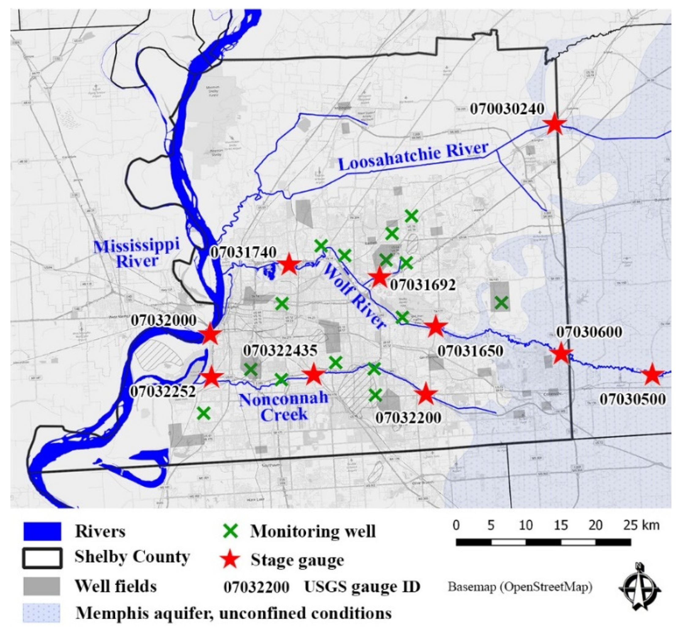
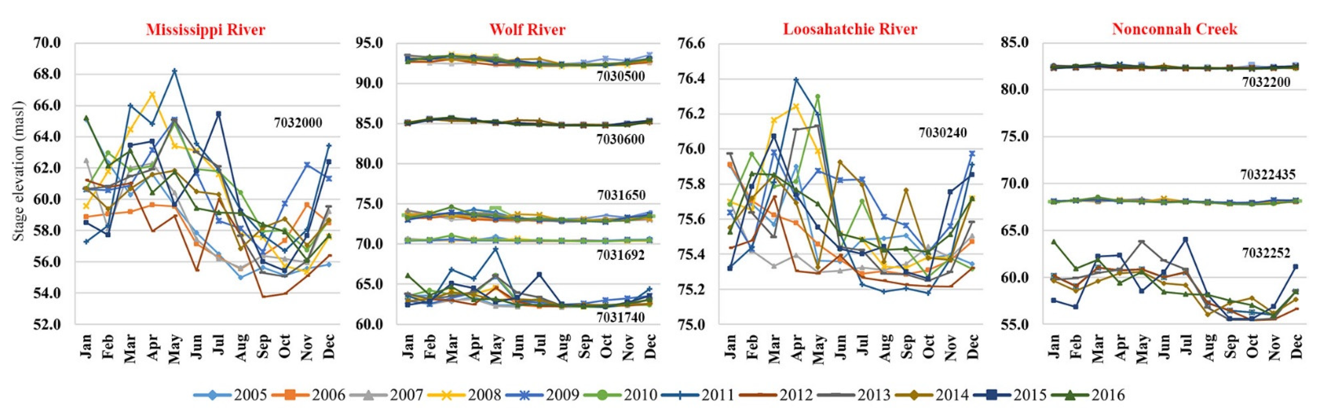
2.1.4. Rivers and Streams
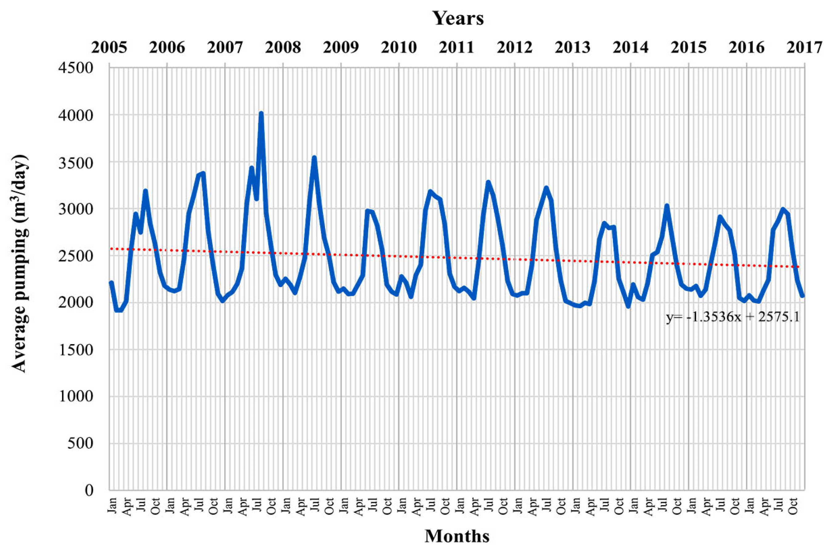
2.1.5. Wells and Groundwater Pumpage
2.2. Calibration
3. Results and Discussion
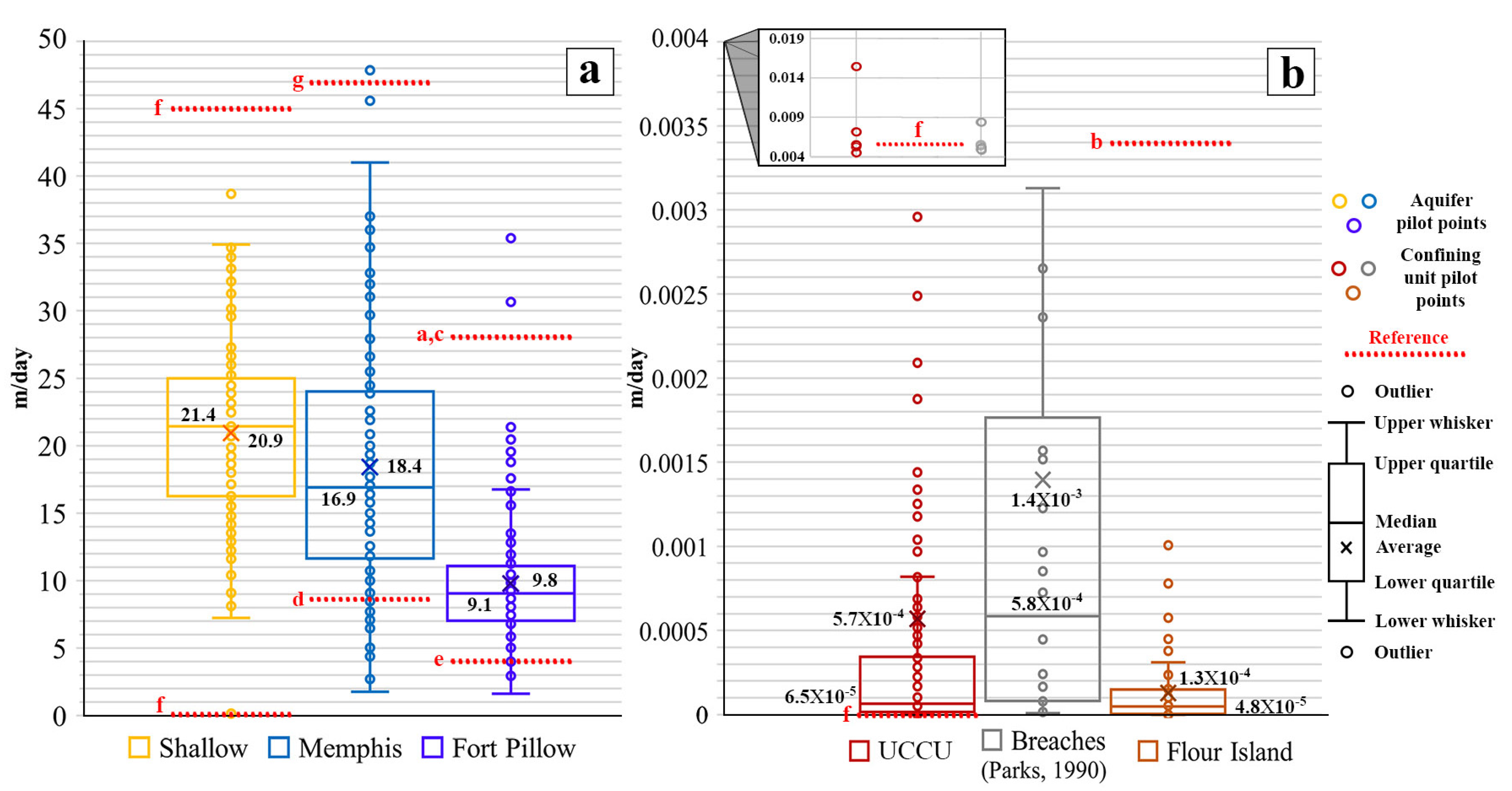
3.1. Hydraulic Parameters
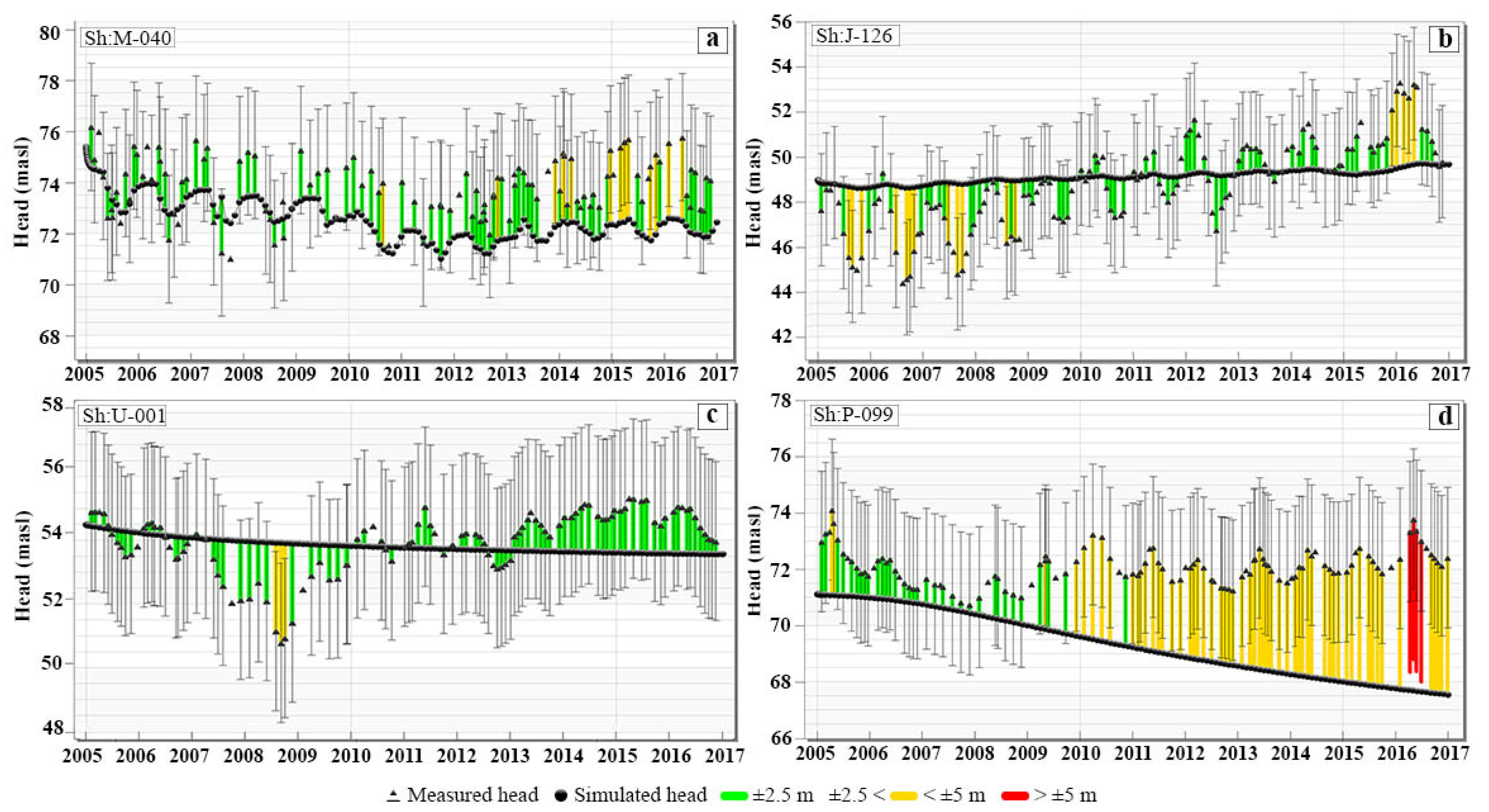
3.2. Model Evaluation
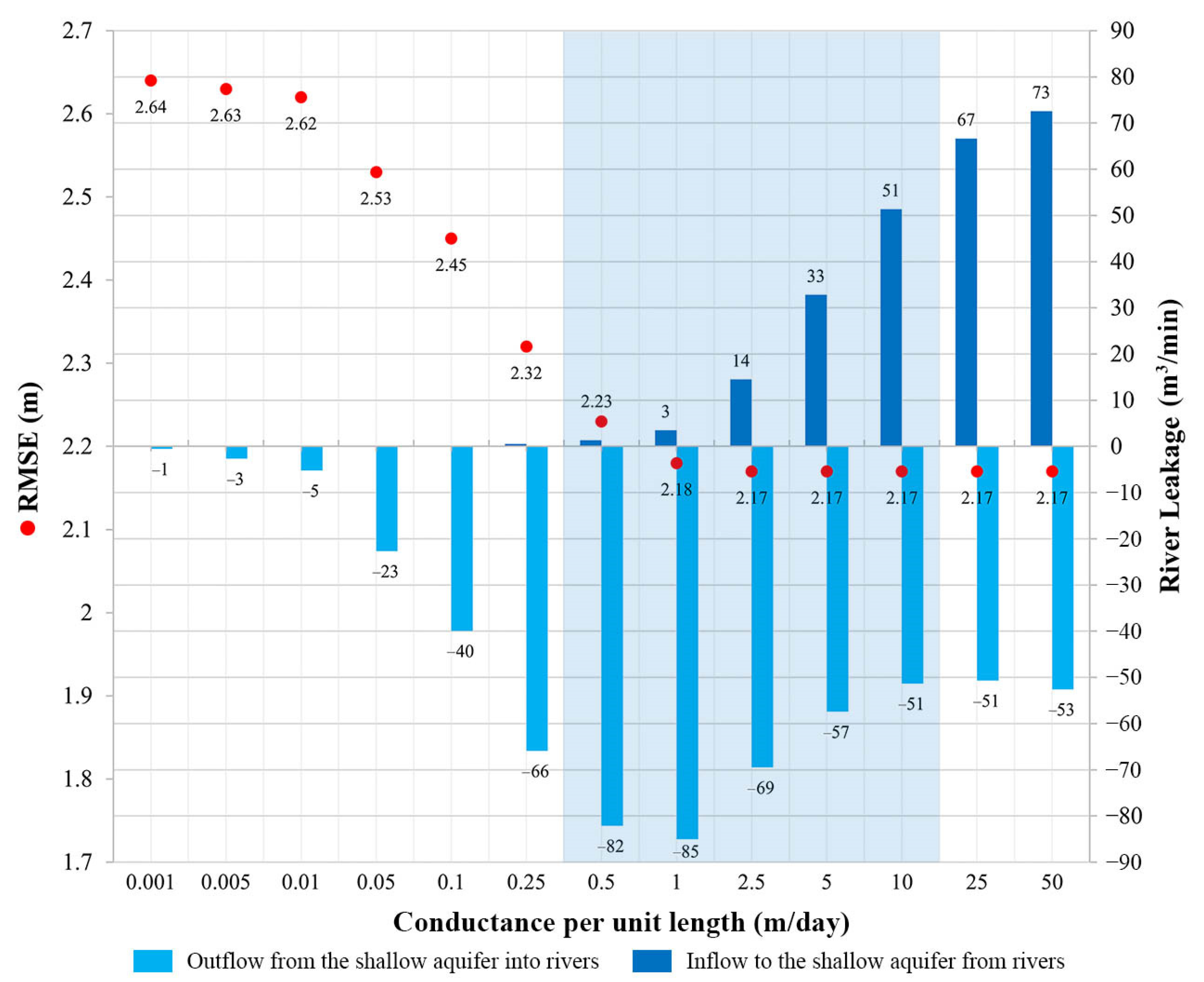
3.3. Flow Budget and Inter-Aquifer Water Exchange
3.4. Multi-Layer Average Daily Flow Budget
3.5. Water Exchanged between the UCCU and the Memphis Aquifer
4. Conclusions and Implications
Supplementary Materials
Author Contributions
Funding
Institutional Review Board Statement
Informed Consent Statement
Data Availability Statement
Acknowledgments
Conflicts of Interest
References
- White, D.E.; Baker, E.T.; Sperka, R. Hydrology of the Shallow Aquifer and Uppermost Semi-Confined Aquifer near El Paso, Texas; Geological Survey Water-Resources Investigations Report 97-4263; U.S. Geological Survey: Austin, TX, USA, 1997; 46p. [CrossRef]
- Lawrence, A.; Gooddy, D.; Kanatharana, P.; Meesilp, W.; Ramnarong, V. Groundwater Evolution Beneath Hat Yai, a Rapidly Developing City in Thailand. Hydrogeol. J. 2000, 8, 564–575. [Google Scholar] [CrossRef] [Green Version]
- Elliot, T.; Chadha, D.S.; Younger, P.L. Water quality impacts and palaeohydrogeology in the Yorkshire Chalk aquifer, UK. Q. J. Eng. Geol. Hydrogeol. 2001, 34, 385–398. [Google Scholar] [CrossRef]
- Parks, W.S. Hydrogeology and Preliminary Assessment of the Potential for Contamination of the Memphis Aquifer in the Memphis Area, Tennessee. U.S. Geological Survey Water-Resources Investigations Report 90-4092; 1990; 39p. Available online: https://pubs.er.usgs.gov/publication/wri904092 (accessed on 27 January 2018).
- Robinson, J.L.; Carmichael, J.K.; Halford, K.J.; Ladd, D.E. Hydrogeologic Framework and Simulation of Ground-water Flow and Travel Time in the Shallow Aquifer System in the Area of Naval Support Activity Memphis, Millington, Tennessee; U.S. Geological Survey Water-Resources Investigations Report 97-4228, 1997; 56p. Available online: https://pubs.er.usgs.gov/publication/wri974228 (accessed on 3 May 2018).
- Larsen, D.; Gentry, R.W.; Solomon, D.K. The geochemistry and mixing of leakage in a semi-confined aquifer at a municipal well field, Memphis, Tennessee, USA. Appl. Geochem. 2003, 18, 1043–1063. [Google Scholar] [CrossRef]
- Waldron, B.A.; Harris, J.B.; Larsen, D.; Pell, A. Mapping an aquitard breach using shear-wave seismic reflection. Hydrogeol. J. 2008, 17, 505–517. [Google Scholar] [CrossRef]
- Barlow, J.R.; Kingsbury, J.; Coupe, R.H. Changes in Shallow Groundwater Quality beneath Recently Urbanized Areas in the Memphis, Tennessee Area. JAWRA J. Am. Water Resour. Assoc. 2012, 48, 336–354. [Google Scholar] [CrossRef]
- Bradley, M.W. Ground-Water Hydrology and the Effects of Vertical Leakage and Leachate Migration on Ground-Water Quality Near the Shelby County Landfill, Memphis, Tennessee. U.S. Geological Survey Water-Resources Investigations Report 90-4075; 1991; 42p. Available online: https://pubs.er.usgs.gov/publication/wri904075 (accessed on 3 May 2018).
- Parks, W.S.; Mirecki, J.E. Hydrogeology, Ground-Water Quality, and Potential for Water-Supply Contamination Near the Shelby County Landfill in Memphis, Tennessee; U.S. Geological Survey Water-Resources Investigations Report 91-4173; 1992; 79p. Available online: https://pubs.er.usgs.gov/publication/wri914173 (accessed on 6 August 2017).
- Doudrick, K.W. A Predictive Model of Groundwater Flow and Contaminant Transport of Cr(VI) and TCE in Collierville, Tennessee. Master’s Thesis, University of Memphis, Memphis, TN, USA, 2008; 98p. [Google Scholar]
- Waldron, B.; Larsen, D.; Hannigan, R.; Csontos, R.; Anderson, J.; Dowling, C.; Bouldin, J. Mississippi Embayment Regional Ground Water Study; U.S. Environmental Protection Agency: Washington, DC, USA, 2011; 220p, EPA/600/R-10/130, 2011.
- Carmichael, J.K.; Kingsbury, J.A.; Larsen, D.; Schoefernacker, S. Preliminary Evaluation of the Hydrogeology and Groundwater Quality of the Mississippi River Valley Alluvial Aquifer and Memphis Aquifer at the Tennessee Valley Authority Allen Power Plants, Memphis, Shelby County, Tennessee. U.S. Geological Survey Open-File Report 2018–1097; 2018; 66p. Available online: https://pubs.er.usgs.gov/publication/ofr20181097 (accessed on 29 June 2019).
- Schoefernacker, S. Evaluation and Evolution of a Groundwater Contaminant Plume at the Former Shelby County Landfill, Memphis, Tennessee. Ph.D. Thesis, University of Memphis, Memphis, TN, USA, 2018; 167p. [Google Scholar]
- Blandford, N.; Blazer, D. Hydrologic Relationships and Numerical Simulations of the Exchange of Water between the Southern Ogallala and Edwards–Trinity Aquifers in Southwest Texas. In Aquifers of the Edwards Plateau; Mace, R.E., Angle, E.S., Mullican, W.F., III, Eds.; Report 360; Texas Water Development Board: Austin, TX, USA, 2004; pp. 115–131. [Google Scholar]
- Proce, J.; Ritzi, R.; Dominic, D.; Dai, Z. Modeling Multiscale Heterogeneity and Aquifer Interconnectivity. Groundwater 2004, 42, 658–670. [Google Scholar] [CrossRef] [PubMed]
- Brunner, P.; Cook, P.; Simmons, C. Hydrogeologic Controls on Disconnection between Surface Water and Groundwater. Water Resour. Res. 2009, 45, W01422. [Google Scholar] [CrossRef] [Green Version]
- Frick, M.; Scheck-Wenderoth, M.; Cacace, M.; Schneider, M. Boundary condition control on inter-aquifer flow in the subsurface of Berlin (Germany)—New insights from 3-D numerical modelling. Adv. Geosci. 2019, 49, 9–18. [Google Scholar] [CrossRef] [Green Version]
- Cognac, K.E.; Ronayne, M.J. Changes to inter-aquifer exchange resulting from long-term pumping: Implications for bedrock groundwater recharge. Hydrogeol. J. 2020, 28, 1359–1370. [Google Scholar] [CrossRef]
- Butler, J.J., Jr.; Tsou, M.-S. Pumping-induced Leakage in a Bounded Aquifer: An Example of a Scale-Invariant Phenomenon. Water Resour. Res. 2003, 39, 1344. [Google Scholar] [CrossRef]
- Huang, Y.; Scanlon, B.R.; Nicot, J.P.; Reedy, R.; Dutton, A.; Kelley, V.; Deeds, N. Sources of Groundwater Pumpage in a Layered Aquifer System in the Upper Gulf Coastal Plain, USA. Hydrogeol. J. 2012, 20, 783–796. [Google Scholar] [CrossRef]
- Jazaei, F.; Waldron, B.; Schoefernacker, S.; Larsen, D. Application of Numerical Tools to Investigate a Leaky Aquitard beneath Urban Well Fields. Water 2019, 11, 5. [Google Scholar] [CrossRef] [Green Version]
- Brahana, J.V. Two-Dimensional Digital Ground-Water Model of the Memphis Sand and Equivalent Units, Tennessee, Arkansas, Mississippi. U.S. Geological Survey Open-File Report 82-99; 1982; 62p. Available online: https://pubs.er.usgs.gov/publication/ofr8299 (accessed on 7 September 2017).
- Arthur, J.K.; Taylor, R.E. Definition of the Geohydrologic Framework and Preliminary Simulation of Ground-water Flow in the Mississippi Embayment Aquifer System, Gulf Coastal Plain, United States. U.S. Geological Survey Water-Resources Investigation Report 86-4364; 1990; 97p. Available online: https://pubs.er.usgs.gov/publication/wri864364 (accessed on 15 February 2018).
- Arthur, J.K.; Taylor, R.E. Ground-Water Flow Analysis of the Mississippi Embayment Aquifer System, South central United States. U.S. Geological Survey Professional Paper 1416-I; 1998; 48p. Available online: https://pubs.er.usgs.gov/publication/pp1416I (accessed on 22 July 2018).
- Brahana, J.V.; Broshears, R.E. Hydrogeology and Groundwater Flow in the Memphis and Fort Pillow Aquifers in the Memphis Area, Tennessee. U.S. Geological Survey Water-Resources Investigations Report 89-4131; 2001; 56p. Available online: https://pubs.er.usgs.gov/publication/wri894131 (accessed on 16 February 2018).
- Clark, B.R.; Hart, R.M. The Mississippi Embayment Regional Aquifer Study (MERAS): Documentation of a Groundwater-Flow Model Constructed to Assess Water Availability in the Mississippi Embayment. U.S. Geological Survey Scientific Investigations Report 2009-5172; 2009; 62p. Available online: https://pubs.er.usgs.gov/publication/sir20095172 (accessed on 1 January 2018).
- Clark, B.R.; Westerman, D.A.; Fugitt, D.T. Enhancements to the Mississippi Embayment Regional Aquifer Study (MERAS) Groundwater-Flow Model and Simulations of Sustainable Water-Level Scenarios. U.S. Geological Survey Scientific Investigations Report 2013-5161; 2013; 29p. Available online: https://pubs.usgs.gov/sir/2013/5161 (accessed on 22 March 2019).
- Krinitzsky, E.L. Geological Investigation of Gravel Deposits in the Lower Mississippi Valley and Adjacent Uplands; Waterways Experiment Station Technical Memorandum no. 3-273; U.S. Army Corps of Engineers: Vicksburg, MS, USA, 1949; 58p.
- Moore, G.K.; Brown, D.L. Stratigraphy of the Fort Pillow Test Well Lauderdale County, Tennessee; Report of Investigations 26 1 sheet; Tennessee Division of Geology: Nashville, TN, USA, 1969.
- Saucier, R.T. Geomorphological Interpretations of Late Quaternary Terraces in Western Tennessee and Their Regional Tectonic Implications; U.S. Geological Survey Professional Paper 1336-A; U.S. Geological Survey: Austin, TX, USA, 1987; 19p. Available online: https://pubs.er.usgs.gov/publication/pp1336A (accessed on 18 May 2018).
- Graham, D.D.; Parks, W.S. Potential for Leakage among Principal Aquifers in the Memphis Area, Tennessee. U.S. Geological Survey Water-Resources Investigations Report 85-4295; 1986; 46p. Available online: https://pubs.er.usgs.gov/publication/wri854295 (accessed on 25 July 2017).
- Carmichael, J.K.; Parks, W.S.; Kingsbury, J.A.; Ladd, D.E. Hydrogeology and Ground-water Quality at the Naval Support Activity Memphis, Near Millington, Tennessee. U.S. Geological Survey Water-Re Investigations Report 97-4158; 1997; 64p. Available online: https://pubs.er.usgs.gov/publication/wri974158 (accessed on 5 June 2018).
- Van Arsdale, R.B.; Bresnahan, R.P.; McCallister, N.S.; Waldron, B. The Upland Complex of the Central Mississippi River Valley: Its Origin, Denudation, and Possible Role in Reactivation of the New Madrid Seismic Zone. In Continental Intraplate Earthquakes: Science, Hazard, and Policy Issues; Special Paper 425; Stein, S., Mazzotti, S., Eds.; Geological Society of America: Boulder, CO, USA, 2007; pp. 177–192. [Google Scholar] [CrossRef]
- Criner, J.H.; Parks, W.S. Historic Water-Level Changes and Pumpage from the Principal Aquifers of the Memphis Area, Tennessee: 1886–1975. U.S. Geological Survey Water-Resources Investigations Report 76-67; 1976; 45p. Available online: https://pubs.er.usgs.gov/publication/wri7667 (accessed on 5 June 2018).
- Kingsbury, J.A. Altitude of the Potentiometric Surfaces, September 1995, and Historical Water-Level Changes in the Memphis and Fort Pillow Aquifers in the Memphis Area, Tennessee. U.S. Geological Survey Water-Resources Investigations Report 96-4278; 1996. Available online: https://pubs.er.usgs.gov/publication/wri964278 (accessed on 6 July 2018).
- Larsen, D.; Waldron, B.; Schoefernacker, S.; Gallo, H.; Koban, J.; Bradshaw, E. Application of Environmental Tracers in the Memphis Aquifer and Implication for Sustainability of Groundwater Resources in the Memphis Metropolitan Area, Tennessee. J. Contemp. Water Res. Educ. 2016, 159, 78–104. [Google Scholar] [CrossRef]
- Kenny, J.F.; Barber, N.L.; Hutson, S.S.; Linsey, K.S.; Lovelace, J.K.; Maupin, M.A. Estimated Use of Water in the United States in 2005; U.S. Geological Survey Circular 1344; 2009; 52p. Available online: https://pubs.usgs.gov/circ/1344/ (accessed on 8 September 2018).
- Dieter, C.A.; Maupin, M.A.; Caldwell, R.R.; Harris, M.A.; Ivahnenko, T.I.; Lovelace, J.K.; Barber, N.L.; Linsey, K.S. Estimated Use of Water in the United States in 2015; U.S. Geological Survey Circular 1441. 2018; 65p. Available online: https://doi.org/10.3133/cir1441 (accessed on 7 August 2020).
- Parks, W.S.; Mirecki, J.E.; Kingsbury, J.A. Hydrogeology, Groundwater Quality, and Source of Ground Water Causing Water-Quality Changes in the Davis Well Field at Memphis, Tennessee. U.S. Geological Survey Water-Resources Investigations Report 94-4212; 1995; 58p. Available online: https://pubs.er.usgs.gov/publication/wri944212 (accessed on 19 September 2018).
- Narsimha, V.K.K. Altitudes of Ground Water Levels for 2005 and Historic Water Level Change in Surficial and Memphis Aquifers, Shelby County, Tennessee. Master’s Thesis, University of Memphis, Memphis, TN, USA, 2007; 54p. [Google Scholar]
- Bradshaw, E.A. Assessment of Ground-water Leakage through the Upper Claiborne Confining Unit to the Memphis Aquifer in the Allen Well Field, Memphis, Tennessee. Master’s Thesis, University of Memphis, Memphis, TN, USA, 2011; 81p. [Google Scholar]
- Gallo, H.G. Hydrologic and Geochemical Investigation of Modern Leakage beneath the McCord Well Field, Memphis, Tennessee. Master’s Thesis, University of Memphis, Memphis, TN, USA, 2015; 55p. [Google Scholar]
- Ogletree, B.T. Geostatistical Analysis of the Water Table Aquifer in Shelby County, Tennessee. Master’s Thesis, University of Memphis, Memphis, TN, USA, 2016; 25p. [Google Scholar]
- Mahon, G.L.; Ludwig, A.H. Simulation of Groundwater Flow in the Mississippi River Alluvial Aquifer in Eastern Arkansas. U.S. Geological Survey Water-Resources Investigations Report 89-4145, 1990; 57p. Available online: https://pubs.er.usgs.gov/publication/wri894145 (accessed on 28 August 2018).
- Ackerman, D.J. Hydrology of the Mississippi River Valley Alluvial Aquifer, South-Central United States. U.S. Geological Survey Professional Paper, 1416-D, 1996; 56p. Available online: https://pubs.er.usgs.gov/publication/pp1416D (accessed on 23 July 2018).
- Stanton, G.P.; Clark, B.R. Recalibration of a Ground-Water Flow Model of the Mississippi River Valley Alluvial Aquifer in Southeastern Arkansas, 1918-1998, With Simulations of Hydraulic Heads Caused by Projected Groundwater Withdrawals Through 2049. U.S. Geological Survey Water-Resources Investigations Report 03-4232; 2003; 48p. Available online: https://pubs.usgs.gov/wri/wri034232/ (accessed on 7 January 2019).
- Schrader, T.P. Potentiometric Surface in the Sparta-Memphis Aquifer of the Mississippi Embayment, Spring 2007. U.S. Geological Survey Scientific Investigations Map 3014. 2008. Available online: https://pubs.er.usgs.gov/publication/sim3014 (accessed on 6 July 2017).
- Lloyd, O.B.; Lyke, W.L. Ground Water Atlas of the United States: Segment 10, Illinois, Indiana, Kentucky, Ohio, Tennessee. U.S. Geological Survey Hydrologic Atlas 730-K; 1995; 30p. Available online: https://pubs.er.usgs.gov/publication/ha730K (accessed on 7 July 2017).
- Anderson, M.P.; Woessner, W.W.; Hunt, R.J. Applied Groundwater Modeling- Simulation of Flow and Advective Transport, 2nd ed.; Academic Press: San Diego, CA, USA, 2015; 630p. [Google Scholar]
- Nyman, J.D. Predicted Hydrologic Effects of Pumping from the Lichterman Well Field in the Memphis Area, Tennessee. U.S. Geological Survey Water Supply Paper 1819-B, 1965; 26p. Available online: https://pubs.er.usgs.gov/publication/wsp1819B (accessed on 25 May 2018).
- Urbano, L.; Waldron, B.; Larsen, D.; Shook, H. Groundwater–surfacewater interactions at the transition of an aquifer from unconfined to confined. J. Hydrol. 2006, 321, 200–212. [Google Scholar] [CrossRef]
- Larsen, D.; Morat, J.; Waldron, B.; Ivey, S.; Anderson, J. Stream Loss Contributions to a Municipal Water Supply Aquifer in Memphis, Tennessee. Environ. Eng. Geosci. 2013, 19, 265–287. [Google Scholar] [CrossRef]
- Schneider, R.; Cushing, E.M. Geology and Water-bearing Properties of the “1400 foot” Sand in the Memphis Area. U.S. Geological Survey Circular 0033; 1948; 13p. Available online: https://pubs.er.usgs.gov/publication/cir33 (accessed on 10 May 2018).
- Parks, W.S.; Carmichael, J.K. Geology and Groundwater Resources of the Fort Pillow Sand in Western Tennessee. U.S. Geological Survey Water-Resources Investigations Report 89-4120. 1989; 20p. Available online: https://pubs.er.usgs.gov/publication/wri894120 (accessed on 11 June 2018).
- Parks, W.S.; Carmichael, J.K. Geology and Ground-water Resources of the Memphis Sand in Western Tennessee. U.S. Geological Survey Water-Resources Investigations Report 88-4182. 1990; 30p. Available online: https://pubs.er.usgs.gov/publication/wri884182 (accessed on 11 June 2018).
- Gentry, R.; McKay, L.; Thonnard, N.; Anderson, J.L.; Larsen, D.; Carmichael, J.K.; Solomon, D.K. Novel Techniques for Investigating Recharge to the Memphis Aquifer; AWWARF Report 91137; American Water Works Association: Denver, CO, USA, 2006; 97p. [Google Scholar]
- Hart, R.M.; Clark, B.R.; Bolyard, S.E. Digital Hydrogeologic Surface and Thickness for the Hydrogeologic Units of the Mississippi Embayment Regional Aquifer Study (MERAS). U.S. Geological Survey Scientific Investigations Report 2008-5098. 2008; 33p. Available online: https://pubs.usgs.gov/sir/2008/5098/ (accessed on 1 November 2017).
- Criner, J.H.; Sun, P.-P.; Nyman, D.J. Hydrology of Aquifer Systems in the Memphis Area, Tennessee. U.S. Geological Survey Water Supply Paper 1779-O, 1964; 31p. Available online: https://pubs.er.usgs.gov/publication/wsp1779O (accessed on 7 August 2018).
- Stantec, 2019. 2018 Annual Groundwater Monitoring and Corrective Action Report. TVA Allen Fossil Plant East Ash Disposal Area CCR Unit. Available online: https://www.tva.com/Environment/Environmental-Stewardship/Coal-Combustion-Residuals/Allen (accessed on 5 February 2020).
- Torres-Uribe, H.E.; Waldron, B.; Larsen, D.; Schoefernacker, S. Application of Numerical Groundwater Model to Determine Spatial Configuration of Confining Unit Breaches near a Municipal Well Field in Memphis, Tennessee. J. Hydrol. Eng. 2021, 26, 05021021. [Google Scholar] [CrossRef]
- Larsen, D.; Brock, C.F. Sedimentology and Petrology of the Eocene Memphis Sand and Younger Terrace Deposits in Surface Exposures of Western Tennessee. Southeast. Geol. 2014, 50, 193–214. [Google Scholar]
- Niswonger, R.G.; Panday, S.; Ibaraki, M. MODFLOW-NWT, A Newton Formulation for MODFLOW-2005. U.S. Geological Survey Techniques and Methods, Book 6 (A37). 2011; 44p. Available online: https://pubs.usgs.gov/tm/tm6a37/ (accessed on 7 April 2017).
- Harbaugh, A.W. MODFLOW-2005, the U.S. Geological Survey Modular Ground-Water Model- The Ground-water Flow Process. U.S. Geological Survey Techniques and Methods, Book 6 (A16). 2005; 253p. Available online: https://pubs.er.usgs.gov/publication/tm6A16 (accessed on 6 April 2017).
- Aquaveo, LLC. Groundwater Modeling System (GMS) Version: 10.3, Aquaveo, UT, USA. 2017. Available online: https://www.aquaveo.com/ (accessed on 1 February 2017).
- Sugarbaker, L.J.; Constance, E.W.; Heidemann, H.K.; Jason, A.L.; Lukas, V.; Saghy, D.L.; Stoker, J.M. The 3D Elevation Program initiative—A call for Action; U.S. Geological Survey Circular 1399. 2014, 35p. Available online: https://pubs.usgs.gov/circ/1399/ (accessed on 17 July 2017).
- U.S. Geological Survey, 3D Elevation Program (3DEP). U.S. Geological Survey, the National Map Web Page. 2017. Available online: http://nationalmap.gov/3DEP/ (accessed on 17 February 2017).
- Schrader, T.P. Water Levels and Water Quality in the Sparta-Memphis Aquifer (Middle Claiborne Aquifer) in Arkansas, Spring-summer 2011. U.S. Geological Survey Scientific Investigations Report 2014-5044. 2014; 44p. Available online: https://pubs.er.usgs.gov/publication/sir20145044 (accessed on 16 February 2018).
- Waldron, B.; Larsen, D. Pre-Development Groundwater Conditions Surrounding Memphis, Tennessee: Controversy and Unexpected Outcomes. JAWRA J. Am. Water Resour. Assoc. 2014, 51, 133–153. [Google Scholar] [CrossRef]
- Brahana, J.V.; Mesko, T.O. Hydrogeology and Preliminary Assessment of Regional Flow in the Upper Cretaceous and Adjacent Aquifers in the Northern Mississippi Embayment. U.S. Geological Survey Water-Resources Investigations Report 87-4000. 1988; 65p. Available online: https://pubs.usgs.gov/wri/wri87-4000 (accessed on 29 June 2018).
- U.S. Geological Survey. USGS Water Data for the Nation—U.S. Geological Survey National Water Information System Web Interface. 2017. Available online: http://waterdata.usgs.gov/nwis/ (accessed on 19 October 2017).
- Freeze, R.A.; Cherry, J.A. Groundwater; Prentice-Hall: Englewood Cliffs, NJ, USA, 1979; 604p. [Google Scholar]
- U.S. Geological Survey. National Hydrography Dataset (NHD). U.S. Geological Survey. 2017. Available online: http://nhd.usgs.gov/ (accessed on 29 June 2017).
- Kingsbury, J.A. Altitude of the Potentiometric Surface, 2000–15, and Historical Water-Level Changes in the Memphis Aquifer in the Memphis area, Tennessee. U.S. Geological Survey Scientific Investigations Map 3415, 1 sheet; 2018. Available online: https://pubs.er.usgs.gov/publication/sim3415 (accessed on 19 November 2018).
- Hill, M.C.; Tiedeman, C.R. Effective Groundwater Model Calibration- With Analysis of Data, Sensitivities, Predictions, and Uncertainty; Wiley and Sons: New York, NY, USA, 2007; 455p. [Google Scholar]
- Doherty, J. PEST: Model-independent Parameter Estimation User Manual Part I, 6th ed.; Watermark Numerical Computing: Corinda, Australia, 2016; 366p. [Google Scholar]
- Fienen, M.N.; Muffels, C.T.; Hunt, R.J. On Constraining Pilot Point Calibration with Regularization in PEST. Groundwater 2009, 47, 835–844. [Google Scholar] [CrossRef]
- Doherty, J.E. Hunt, Approaches to Highly Parameterized Inversion—A Guide to Using PEST for Groundwater-Model Calibration. U.S. Geological Survey Scientific Investigations Report 2010-5169. 2010; 59p. Available online: https://pubs.usgs.gov/sir/2010/5169/ (accessed on 16 July 2018).
- Doherty, J.E.; Fienen, M.N.; Hunt, R.J. Approaches to Highly Parameterized Inversion- Pilot-Point Theory, Guidelines, and Research Directions. U.S. Geological Survey Scientific Investigations Report 2010-5168. 2010; 36p. Available online: https://pubs.er.usgs.gov/publication/sir20105168 (accessed on 16 July 2018).
- Kalman, D. A Singularly Valuable Decomposition: The SVD of a Matrix. Coll. Math. J. 1996, 27, 2–23. [Google Scholar] [CrossRef]
- Tikhonov, A.N.; Arsenin, V.I.A. Solution of Ill-posed Problems; Halsted: New York, NY, USA, 1977; 258p. [Google Scholar]
- Tonkin, M.J.; Doherty, J. A hybrid regularized inversion methodology for highly parameterized environmental models. Water Resour. Res. 2005, 41, W10412. [Google Scholar] [CrossRef] [Green Version]
- Hunt, R.J.; Doherty, J.; Tonkin, M.J. Are Models Too Simple? Arguments for Increased Parameterization. Groundwater 2007, 45, 254–262. [Google Scholar] [CrossRef]
- Doherty, J. Ground Water Model Calibration Using Pilot Points and Regularization. Groundwater 2003, 41, 170–177. [Google Scholar] [CrossRef] [PubMed]
- Hunt, R.J.; Zheng, C. The Current State of Modeling. Groundwater 2012, 50, 330–333. [Google Scholar] [CrossRef]
- Larsen, D.; Bursi, J.; Waldron, B.; Schoefernacker, S.; Eason, J. Recharge pathways and rates for a sand aquifer beneath a loess-mantled landscape in western Tennessee, U.S.A. J. Hydrol. Reg. Stud. 2020, 28, 100667. [Google Scholar] [CrossRef]
- Simco, W.A. Recharge of the Memphis Aquifer in an Incised Urban Watershed. Master’s Thesis, University of Memphis, Memphis, TN, USA, 2018; 49p. [Google Scholar]
- Smith, S.R. Recharge of the Memphis Aquifer in an Incised Urban Watershed: Implications of Impervious Surfaces and Stream Incision. Master’s Thesis, University of Memphis, Memphis, TN, USA, 2019; 68p. [Google Scholar]
- Bouzeid, S. Factors Influencing Recharge to the Memphis Aquifer in an Urban Watershed. Master’s Thesis, University of Memphis, Memphis, TN, USA, 2021; 47p. Unpublished Manuscript. [Google Scholar]
- Kenley, D.W. A Ground Water Flow Model of the Northern Mississippi Embayment. Master’s Thesis, University of Memphis, Memphis, TN, USA, 1993; 91p. [Google Scholar]
- McKee, P.W.; Clark, B.R. Development and Calibration of a Ground-water Flow Model for the Sparta Aquifer of Southeastern Arkansas and North-Central Louisiana and Simulated Response to Withdrawals, 1998–2027. U.S. Geological Survey Water-Resources Investigations Report 03-4132; 2003; 71p. Available online: https://pubs.er.usgs.gov/publication/wri034132 (accessed on 7 August 2018).
- Langevin, C.D.; Hughes, J.D.; Banta, E.R.; Niswonger, R.G.; Panday, S.; Provost, A.M. MODFLOW 6-Description of Input and Output, Documentation for the MODFLOW 6 Groundwater Flow Model. U.S. Geological Survey Techniques and Methods, mf6io and 6-A55, 188 and 197p; 2017. Available online: https://pubs.er.usgs.gov/publication/tm6A55 (accessed on 7 August 2018).
- Czarnecki, J.B.; Gillip, J.A.; Jones, P.M.; Yeatts, D.S. Groundwater-Flow Model of the Ozark Plateaus Aquifer System, Northwestern Arkansas, Southeastern Kansas, Southwestern Missouri, and Northeastern Oklahoma. U.S. Geological Survey Scientific Investigations Report 2009-5148. 2009; 62p. Available online: https://pubs.usgs.gov/sir/2009/5148/ (accessed on 21 June 2018).
- Masterson, J.P.; Pope, J.P.; Fienen, M.N.; Monti, J.; Nardi, M.R.; Finkelstein, J.S. Documentation of a Groundwater Flow Model Developed to Assess Groundwater Availability in the Northern Atlantic Coastal Plain Aquifer System from Long Island, New York, to North Carolina. U.S. Geological Survey Scientific Investigations Report 2016–5076. 2016; 70p. Available online: https://pubs.er.usgs.gov/publication/sir20165076 (accessed on 21 June 2018).
- Koban, J.; Larsen, D.; Ivey, S. Resolving the source and mixing proportions of modern leakage to the Memphis aquifer in a municipal well field using geochemical and 3H/3He data, Memphis, Tennessee, USA. Environ. Earth Sci. 2011, 66, 295–310. [Google Scholar] [CrossRef]
- Gentry, R.W.; Larsen, D.; Ivey, S.S. Efficacy of GA to Investigate Small Scale Aquitard Leakage. J. Hydraul. Eng. 2003, 129, 527–535. [Google Scholar] [CrossRef]
- Smith, M.R. Evaluating Modern Recharge to the Memphis Aquifer at the Lichterman Well Field, Memphis, Tennessee. Master’s Thesis, University of Memphis, Memphis, TN, USA, 2018; 90p. [Google Scholar]


| System and Series | Group | Stratigraphic Unit | Hydro- Stratigraphic Unit | Thickness (m) | Lithology | Model Layer | Hydraulic Conductivity (m/day) | ||
|---|---|---|---|---|---|---|---|---|---|
| Min | Max | ||||||||
| Quaternary | Holocene and Pleistocene | Alluvium | shallow (alluvial) aquifer | 0–50 | Sand, gravel, silt, and clay. Underlies the Mississippi River alluvial plain and alluvial plains of tributary streams in western Tennessee. Thickest beneath the Mississippi River alluvial plain, where commonly between 30 and 45 m thick; generally, less than 15 m thick elsewhere. | 1 | 2.5 × 10⁻⁵ f | 45 f | |
| Pleistocene | Loess | Leaky confining unit | 0–20 | Silt, silty clay, and minor sand. Principal unit at the surface in upland areas of western Tennessee. Thickest on the bluffs that border the Mississippi alluvial plain; thinner eastward from the bluffs. | |||||
| Quaternary and Tertiary | Pleistocene and Pliocene (?) | Fluvial terrace deposits | shallow (Fluvial) aquifer | 0–30 | Sand, gravel, minor clay, and ferruginous sandstone. Generally, underlies the loess in upland areas, but locally absent. Thickness varies greatly because of erosional surfaces at top and base. | ||||
| Tertiary | Eocene | Claiborne | Jackson Formation | upper Claiborne confining unit | 0–110 | Clay, silt, sand, and lignite. Because of similarities in lithology, the Jackson Formation and upper part of the Claiborne Group cannot be reliably subdivided based on available information. Most of the preserved sequence is the Cockfield and Cook Mountain Formations undivided. | 2 | 1.5 × 10⁻⁶ f | 6.0 × 10⁻³ f |
| Cockfield and Cook Mountain formations | |||||||||
| Memphis Sand | Memphis aquifer | 150–270 | Sand, clay, and minor lignite. Thick body of sand with lenses of clay at various stratigraphic horizons and minor lignite. Thickest in the southwestern part of the Memphis area; thinnest in the northeastern part. | 3–6 | 8.5 d | 47 g | |||
| Eocene(?) | Wilcox | Flour Island Formation | Flour Island confining unit | 50–95 | Clay, silt, sand, and lignite. Consists primarily of silty clays and sandy silts with lenses and interbedded fine sand and lignite. | 7 | 3.5 × 10⁻³ b | ||
| Paleocene | Fort Pillow Sand | Fort Pillow aquifer | 40–95 | Sand with minor clay and lignite. Sand is fine to medium grained. Thickest in the southwestern part of the Memphis area; thinnest in the northern and northeastern parts. | 8 | 4 e | 28 a,c | ||
| Midway | Old Breastworks Formation | Old Breastworks confining unit | 55–110 | Clay, silt, sand, and lignite. Consists primarily of silty clays and clayey silts with lenses and interbedded fine sand and lignite. | No-Flow Boundary | ||||
| Location | Wells 1 | Aquifer | Average Depth (m) | Screen Length (m) |
|---|---|---|---|---|
| Bartlett | 11 | M | 150 | 30 |
| Collierville | 12 | M | 100 | 20 |
| Germantown | 20 | M | 120 | 20 |
| Millington | 2 | M | 105 | 20 |
| 4 | F.P | 460 | 20 | |
| Allen | 27 | M | 140 | 30 |
| Davis | 19 | M | 140 | 25 |
| Lichterman | 23 | M | 145 | 30 |
| LNG | 2 | M | 115 | 30 |
| Mallory | 24 | M | 190 | 30 |
| McCord | 27 | M | 165 | 30 |
| Morton | 17 | M | 165 | 35 |
| Palmer | 4 | M | 120 | 25 |
| Shaw | 14 | M | 195 | 35 |
| 3 | F.P | 360 | 35 | |
| Sheahan | 24 | M | 170 | 30 |
| DeSoto | 84 | M | 105 | 20 |
| 9 | F.P | 445 | 30 |
| Vertical Discretization | Average Layer Thickness (m) | Wells > 80% Screen |
|---|---|---|
| 3 layers | 77 | 70% |
| 4 layers | 58 | 72% |
| 5 layers | 46 | 63% |
| 6 layers | 39 | 50% |
| 7 layers | 33 | 57% |
| Measure of Error (m) | Entire Model | Shallow | Memphis | Fort Pillow | |
|---|---|---|---|---|---|
| Monitoring wells | This model | 74 | 15 | 46 | 13 |
| Mean error | 0.0 | 0.1 | 0.4 | −0.8 | |
| Mean absolute error | 1.6 | 1.8 | 1.4 | 1.8 | |
| RMSE | 2.0 | 2.2 | 1.8 | 2.3 | |
| Reference | Shallow | Memphis | Fort Pillow | ||
| Previous models RMSE | h | NM | ±1.5 * | NM | |
| i | NM | ~16 | ~11 | ||
| j | NM | 11.5 | 10.3 | ||
| k | NM | 4.3 | 3.0 | ||
| l | NM † | 10.9 | NR | ||
| m | NM † | 9.8 | NR | ||
Publisher’s Note: MDPI stays neutral with regard to jurisdictional claims in published maps and institutional affiliations. |
© 2021 by the authors. Licensee MDPI, Basel, Switzerland. This article is an open access article distributed under the terms and conditions of the Creative Commons Attribution (CC BY) license (https://creativecommons.org/licenses/by/4.0/).
Share and Cite
Villalpando-Vizcaino, R.; Waldron, B.; Larsen, D.; Schoefernacker, S. Development of a Numerical Multi-Layered Groundwater Model to Simulate Inter-Aquifer Water Exchange in Shelby County, Tennessee. Water 2021, 13, 2583. https://doi.org/10.3390/w13182583
Villalpando-Vizcaino R, Waldron B, Larsen D, Schoefernacker S. Development of a Numerical Multi-Layered Groundwater Model to Simulate Inter-Aquifer Water Exchange in Shelby County, Tennessee. Water. 2021; 13(18):2583. https://doi.org/10.3390/w13182583
Chicago/Turabian StyleVillalpando-Vizcaino, Rodrigo, Brian Waldron, Daniel Larsen, and Scott Schoefernacker. 2021. "Development of a Numerical Multi-Layered Groundwater Model to Simulate Inter-Aquifer Water Exchange in Shelby County, Tennessee" Water 13, no. 18: 2583. https://doi.org/10.3390/w13182583