
Multiple-Depth Soil Moisture Estimates Using Artificial Neural Network and Long Short-Term Memory Models
by
 , , , and
Heechan Han
1 ,
,
Changhyun Choi
2,
Jongsung Kim
3,
Ryan R. Morrison
4 ,
,
Jaewon Jung
5 and
Hung Soo Kim
3,* 1
Blackland Extension and Research Center, Texas A&M AgriLife, Temple, TX 76502, USA
2
Risk Management Office, KB Claims Survey and Adjusting, Seoul 04027, Korea
3
Department of Civil Engineering, Inha University, Incheon 22212, Korea
4
Department of Civil and Environmental Engineering, Colorado State University, Fort Collins, CO 80523, USA
5
Institute of Water Resources System, Inha University, Incheon 22212, Korea
*
Author to whom correspondence should be addressed.
Water 2021, 13(18), 2584; https://doi.org/10.3390/w13182584
Submission received: 12 August 2021
/
Revised: 13 September 2021
/
Accepted: 16 September 2021
/
Published: 18 September 2021
(This article belongs to the Special Issue The Application of Artificial Intelligence in Hydrology)
Abstract
:Accurate prediction of soil moisture is important yet challenging in various disciplines, such as agricultural systems, hydrology studies, and ecosystems studies. However, many data-driven models are being used to simulate and predict soil moisture at only a single depth. To predict soil moisture at various soil depths with depths of 100, 200, 500, and 1000 mm from the surface, based on the weather and soil characteristic data, this study designed two data-driven models: artificial neural networks and long short-term memory models. The developed models are applied to predict daily soil moisture up to 6 days ahead at four depths in the Eagle Lake Observatory in California, USA. The overall results showed that the long short-term memory model provides better predictive performance than the artificial neural network model for all depths. The root mean square error of the predicted soil moisture from both models is lower than 2.0, and the correlation coefficient is 0.80–0.97 for the artificial neural network model and 0.90–0.98 for the long short-term memory model. In addition, monthly based evaluation results showed that soil moisture predicted from the data-driven models is highly useful for analyzing the effects on the water cycle during the wet season as well as dry seasons. The prediction results can be used as basic data for numerous fields such as hydrological study, agricultural study, and environment, respectively.
1. Introduction
Soil moisture is a component of the natural hydrological cycle that is influenced by rainfall, evapotranspiration, runoff, and fluctuations in the groundwater level, and it is an important element that links climate, soil, and vegetation in this cycle. It is defined as the moisture present in soil voids (space between soil particles) and controls the water–energy exchange between the soil and the atmosphere, accounting for approximately 0.0001% of the surface water [1]. Due to the high variability of soil moisture, it is very important to understand changes in its spatial and temporal distribution. This information can be used in many areas, such as weather forecasting, drought monitoring, runoff forecasting, flood control, yield estimation, and reservoir management [2,3,4,5,6,7]. In certain fields, soil moisture must be understood according to the soil depth. For example, for efficient yield management, it is important to obtain the soil moisture information at relatively varied depths because the root depth varies according to the crop type [8]. As the effect of soil moisture, layer-by-layer, on flooding and drought varies in terms of hydrology, it is essential to analyze the soil moisture at various depths rather than at specific depths.
There are two types of methodologies for measuring soil moisture content: direct and indirect methods. The gravimetric method, which derives the moisture content from the weight difference of the collected soil samples before and after drying, is a typical direct method. The indirect methods include those using a neutron probe, time-domain reflectometry, and psychrometry [9,10]. However, to understand the spatial variability of soil moisture throughout a region, soil moisture should be measured on a site-by-site or point-by-point basis, using gravitational, nuclear, electromagnetic, tension, and humidity techniques over a wide geographical area, which requires considerable time and expensive equipment. For this reason, various physical models capable of predicting the amount of soil moisture, such as the National Water Model (NWM), soil-plant-atmosphere-water model (SPAW), the U.S. Department of Agriculture Hydrograph Laboratory model (USDAHL), and Sacramento-soil moisture accounting model (SAC-SMA) have been developed and used [11,12,13].
To improve the quality of soil moisture prediction, techniques for predicting soil moisture using a remote sensing system have been developed, which can provide a wide range of practical information [14,15,16,17]. However, when predicting soil moisture using a remote sensing system, a downscaling technique is required owing to the low spatial resolution of the remote sensing system. Parinussa et al. [18] combined images of high- and low-resolution measurement data and applied downscaling by using the smoothing filter-based intensity modulation method. Chauhan et al. [19] downscaled the soil moisture data using the special sensor microwave/imager and the advanced very high-resolution radiometer data, with NDVI, land-surface temperature, and surface albedo used as the parameters. Using this method, Ray et al. [20] downscaled the 25-km soil moisture data obtained by the Advanced Microwave Scanning Radiometer on the Earth Observing System to 1 km and compared them with the soil moisture data derived from the VIC-3L-model, which is a physical/dynamic model. However, conventional measuring methods have limitations in that the prediction reliability is reduced due to problems such as the increased observation period, obsolescence of observation equipment, and missing points, as well as the requirement of considerable time, manpower, and money. In addition, the soil moisture data derived from remote sensing have limitations in terms of the lattice size and observation depth and need to be calibrated as they are significantly influenced by factors such as vegetation cover, soil temperature, and terrain. To overcome these limitations, various data-driven models have recently been studied to estimate soil moisture.
With the recent development in computer technology, various models for estimating soil characteristics, such as soil temperature and soil moisture, are being developed by applying data-driven models such as artificial neural network (ANN), support vector machine (SVM), and long short-term memory (LSTM) models. The main concept of data-driven models, such as machine learning, is to determine the relationship between input and output variables in the absence of a clear understanding of the physical process of a certain system. These methods can be more effective than physical or dynamic models for solving complex and nonlinear problems [21]. James et al. [22] applied convolutional neural networks (CNN) for water segmentation using satellite imagery. The results have shown that CNN is suitable for contributing to the wider use of satellite imagery for water management. Furthermore, Kim et al. [23] applied a multilayer perceptron (MLP) and an adaptive neuro-fuzzy inference system to predict the daily soil temperature at two observation points (Champaign and Springfield stations) located in Illinois, USA. A comparison of the simulation results with the observed data confirmed that both models appropriately predicted the soil temperature. Feng et al. [24] confirmed the applicability of various machine learning methods (extreme learning machine (ELM), generalized regression neural networks, backpropagation neural networks, and random forest (RF)) using meteorological factors to predict soil temperature according to the soil depth. As a result of the analysis, all models led to statistically significant results, and in particular, the ELM model was excellent in terms of performance and computational speed. In addition, Sutskever et al. [25] presented improved sequence-based data analysis results using a sequence-to-sequence structure that can consider temporal dependence on the LSTM model (LSTM-s2s). Various studies have been conducted to develop prediction models for soil moisture and soil temperature based on data-driven models [26,27,28]. Gill et al. [29] developed two models to predict soil moisture by applying SVM and ANN and compared their performances. Consequently, although both models performed well, SVM showed a better performance. Prakash et al. [30] predicted soil moisture using machine learning techniques, multiple linear regression, support vector regression (SVR), and recurrent neural networks; evaluated the predictive power using mean square error (MSE) and R2; and confirmed the applicability of various machine learning models for soil moisture prediction. Achieng [31] predicted and evaluated soil moisture using machine learning techniques such as the radial basis function (RBF), single-layer ANN, and deep neural network, among which RBF was found to be outstanding. Adeyemi et al. [32] predicted soil moisture through dynamic neural network modeling. The model was trained to generate a one-day-ahead prediction of the volumetric soil moisture content based on the previously conducted soil moisture, precipitation, and climatic measurements. In their study, the field data obtained from three sites were used for the prediction, and an R2 value of above 0.94 was obtained in all sites through the model evaluation. Other studies have been conducted for the prediction and evaluation of soil moisture using a machine learning technique and comparison with existing methods [33,34,35,36].
However, in previous studies, since soil moisture at a single depth was simulated and predicted, it is difficult to recognize the performance of the data-driven models for soil moisture prediction at various depths from surface to deep layers. To address these limitations, this study aims to develop prediction models to estimate soil moisture at multiple depths by considering machine learning techniques (i.e., ANN) and deep learning techniques (i.e., LSTM).
2. Materials and Methods
2.1. Study Area and Data
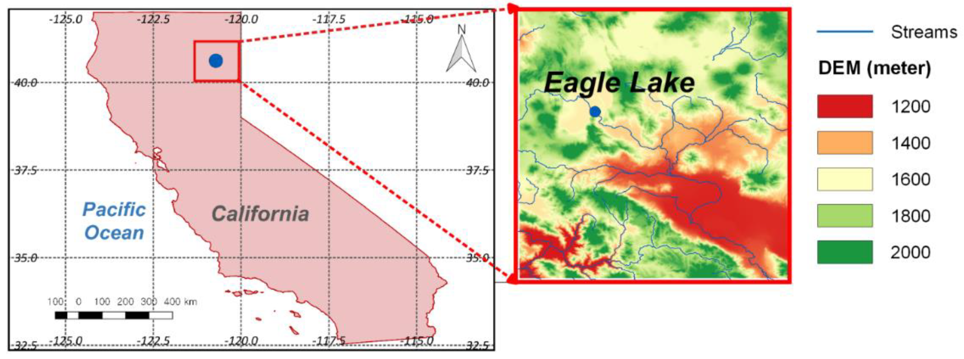
The Eagle Lake catchment (40°37′ N latitude, 120°43′ W longitude), located in California, USA, was designated as the study area (Figure 1). The hydrological data in this area are in high demand due to the annual flood and drought damage caused by various topographic and climate phenomena. Since flooding and drought are highly related to soil moisture [37], it is important to observe and manage the soil moisture data to reduce the damage. The average annual precipitation in the region is 550 mm, where over 90% of the precipitation occurs from November to March. In addition, large amounts of rainfall are generated in the region from extratropical cyclones or jet streams from the Pacific Ocean [38], and heavy rains are generated from atmospheric rivers during the rainy season [39,40].
In this study, five variables provided by the Soil Climate Analysis Network (SCAN), containing air temperature, precipitation, vapor pressure, soil temperature, and relative humidity, were used as input data for each model to predict soil moisture at four depths. These data were collected on a daily time scale from November 2014 to February 2020 at an observation station located in Eagle Lake (Figure 1). In the SCAN monitoring system, the dielectric constant measuring device was used for measuring soil moisture at multiple depths. In this study, the soil temperature and soil moisture data were collected from four layers at the monitoring site, with depths of 100, 200, 500, and 1000 mm from the surface, for predicting the soil moisture at various depths. In this study, approximately 70% (November 2014 to June 2018) of the total data were used for training the model, and the remaining 30% (July 2018 to February 2020) were used for testing.
2.2. Methods
2.2.1. Long Short-Term Memory Model (LSTM)
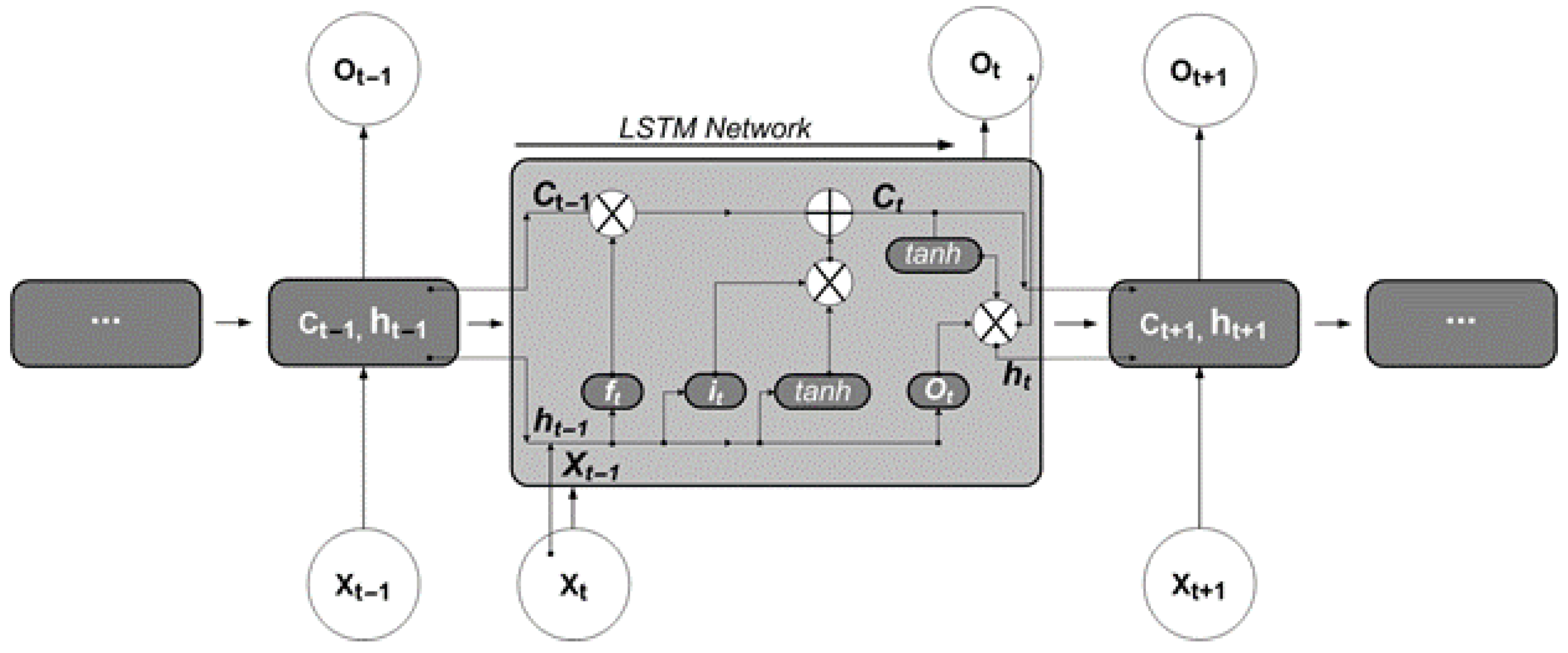
Long short-term memory (LSTM), introduced by Hochreiter and Schmidhuber (1997) [41], is a deep learning model based on a recurrent neural network (RNN), which was developed to solve the problem of gradient vanishing or gradient exploding of the error slope in the RNN model when analyzing long-term data. LSTM model is used for learning continuously composed data, mainly for purposes such as language translation and speech pattern recognition. In the field of hydrology, it is used for prediction through learning the hydrological time-series data, such as runoff prediction [42,43,44] and water-level prediction [45]. Figure 2 shows the structure and conceptual diagram of LSTM.
LSTM is composed of several blocks, each of which comprises cells that can maintain their state with time and three nonlinear gates that control the data flow (Figure 2). The three gates are the forget gate (ft; Equation (6)), input gate (it; Equation (7)), and output gate (ot; Equation (8)). The forget gate can determine how much of the information from the previous block should be retained. The purpose of the input gate is to determine which of the new information is stored in the cell. The output gate determines the final output value among the information stored in the cell. The LSTM algorithm is operated from an input sequence data Xt to final outcome Ot by looping through Equations (1)–(6) with initial values of C0 = 0 and h0 = 0 [32].
where σ is the nonlinear activation function. Wf, Wi, Wo, and Wc are weight values of forget gate, input gate, output gate, and memory cells, ht−1 denotes output data from the previous cell, xt is current input data, and bf, bi, and bo are bias vectors of each gate, respectively. In addition, is the state of any cell generated from the activation function. In this study, Rectified Linear Unit (Relu) functions were used as activation functions.
As the calculation process of LSTM is based on various parameters, it is somewhat more complicated and time-consuming than the other models but presents a high-performance result. In addition, unlike other models, it is very useful for learning the relation of long-term data because it uses the concept of a cell to store and update information selectively according to the previous state and current input [46,47]. The LSTM model is available as standard packages in various software programs, and the Keras framework in the Python 3.4 was used to operate the models in this study.
2.2.2. Artificial Neural Network (ANN)
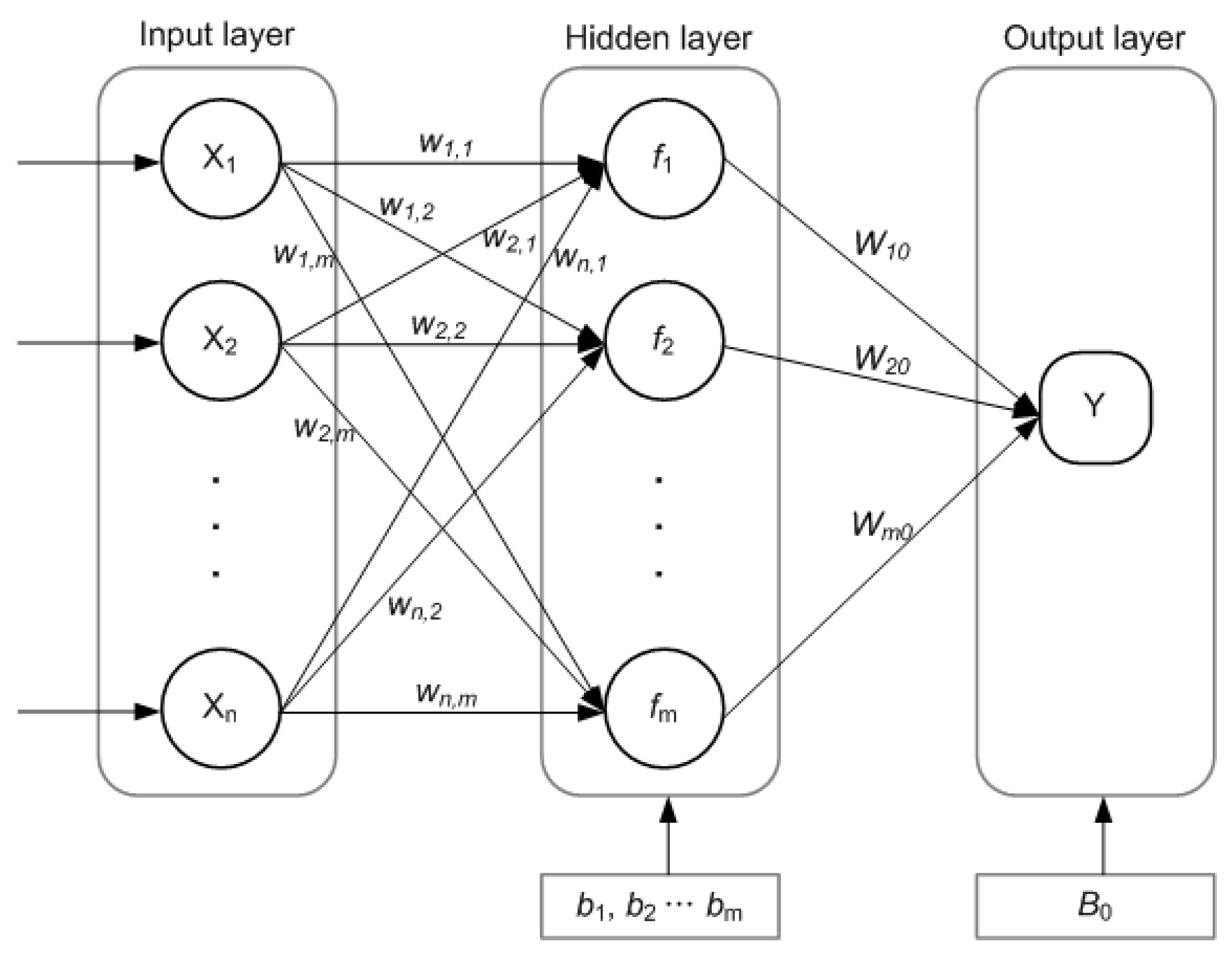
McCulloch and Pitts (1943) introduced the ANN model, which is a supervised machine learning algorithm. Generally, the ANN model is applied to solve problems for the classification and prediction of specific variables that have undefined mathematical relationships. The ANN model is described as a mathematical structure capable of representing the complex and nonlinear process correlating the input and output of the system [48]. The ANN model has shown desirable performance for the analysis of nonlinear relationships between independent and dependent variables in a given data set [49]. Figure 3 represents the conceptual diagram of the ANN model.
The initial ANN model is a single-layer perceptron containing one input and output layer. It is known as an effective method for linear separation, but it has the limitation that it is hard to solve nonlinear problems [50]. To overcome this limitation, Multi-Layer Perceptron (MLP), one of the most common neural network models, was implemented. The MLP is a class of ANN model and is a complex network that consists of three different types of layers, including input, hidden, and output layers (Figure 3). Since the ANN with multiple layers was used, it can be called ANN, MLP, or ANN-MLP models (In this study, the ANN term is used). These three layers contain sets of neurons that are fully connected with neurons in the following layer, and each layer has different weight values. The ANN model was designed to reduce the difference between estimated and targeted values by the process of adjusting the parameters of the model. The ANN model can be mathematically formulated as following Equation (7).
where f denotes the activation function in the layers, and X, w represent the input value and weight values between layers. B and b indicate the biases in the output and hidden layers. In the model algorithm, the X can be multiplied by the weight value (w), and then the coupled value is converted by the activation function (f). The representative activation functions used in the ANN model include sigmoid, hyperbolic tangent function (tanh), and Relu functions. In this study, the Relu function was used as an activation function for the ANN model.
2.3. Model Development
In order to predict soil moisture for each layer at t + n time points, the historical observation data from t − m to t time points were used as input for each model. Soil moisture at four layers was predicted using Equation (8):
where S is the soil moisture value, I indicates input variables, k is the number of input variables, and l denotes the four layers. m means the previous time steps of input data, n is the prediction time. In this study, the observed meteorological and soil moisture data from the previous 12 days were used as input data to predict soil moisture from 1 to 6 days ahead.
The collected input data required two pre-processing steps. The first step is to supplement the missing values of the data generated during the observation, to enhance the data continuity. The process of supplementing the missing values is essential for the data-driven models, as the temporal continuity of the data is very important. In this study, a missing value was substituted with the average value of the soil moisture data before and after the time step. The second pre-processing step involved data normalization. As the unit and range of each data set differ in each model, the function values are very likely to diverge, thus degrading the simulation performance. Therefore, in this study, all input data were converted to values between 0 and 1 through the normalization process (Equation (9)), as follows:
where Zi is the normalized variable, Xi is the actual variable, and Xmax and Xmin are the maximum and minimum values of the variable, respectively.
2.4. Evaluation Methods
In this study, the correlation coefficient (CC), root mean square error (RMSE), Nash–Sutcliffe efficiency (NSE), and relative error (RE) were used to evaluate the predictive performance of models applied for soil moisture prediction. CC is an index indicating the degree of the linear relation between the actual and predicted values. A CC value close to one indicates that the two variables have a very strong positive linear relation. RMSE is the standard deviation of the prediction error, which is a difference between predicted results and observation. As the value of RMSE is closer to zero, the prediction can be determined to be more accurate with fewer errors. In addition, the NSE value of one indicates that the model perfectly simulates the observed value, and a value less than zero means that the average observed value is better than simulated results. RE denotes the ratio of the difference between simulated and observed values to the observation. RE value of zero means the best performance of simulated results. Equations (10)–(13) indicate the formula for CC, RMSE, NSE, and RE, respectively.
where Yobs is the actual value, Ypre is the predicted value derived from the model, and are the averaged value of Yobs and Ypre. n is the number of data sets.
3. Results
3.1. Comparison with Observations at Four Layers
In this study, the quality of daily soil moisture at four layers, predicted from the LSTM and ANN models, was evaluated through a comparison with the soil moisture observed at the soil moisture station in Eagle Lake. The evaluation was conducted on the daily soil moisture data observed between July 2018 and February 2020.
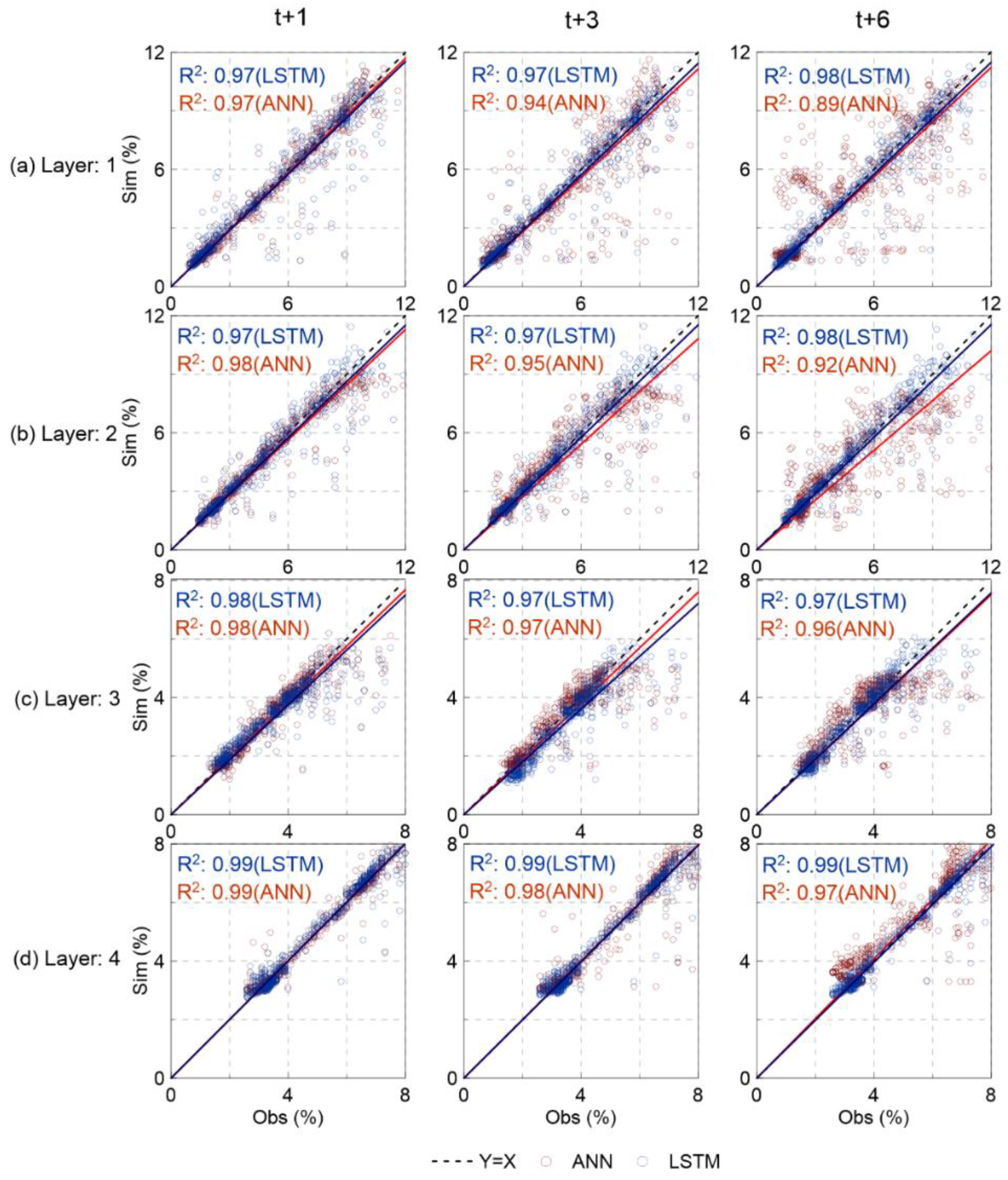
Figure 4 shows scatter plots of the observed soil moisture and predicted results from the two models (i.e., ANN and LSTM) for the four layers. All data-driven models predicted soil moisture values acceptably, compared with the observed values. The comparison results show that the LSTM model provides relatively better performance than the ANN model for all depths. In addition, the predictive performance of the ANN model seems to decrease as the lead time increases from 1 to 6 days. For example, for a lead time of 6 days, the points representing soil moisture predicted from the ANN model appear to be relatively far apart on the X = Y line. Moreover, it was found that the simulation performance for the soil moisture of the surface layer was relatively worse than that of the deep layer. It can be inferred that the large temporal variability of soil moisture in the surface layer than in the deep layer affected the simulation results.
In this study, three statistical factors (e.g., CC, RMSE, and NSE) were used for the statistical evaluation of the performance of the two models for soil moisture prediction. With these factors, the prediction performance of the models, based on the predicted amount and tendency of soil moisture, was compared with the observed data. Table 1 shows statistical metrics for the soil moisture predicted from the two data-driven models, LSTM and ANN models. The prediction performance of the two models was found to be generally acceptable based on the statistical factors. The statistical metrics showed that the LSTM model showed relatively better predictive performance than the ANN model in all layers. Considering that the CC values were ranged from 0.80 to 0.97 for ANN and from 0.90 to 0.98 for the LSTM model, the RMSE value was lower than 2.0, and the NSE values were ranged from 0.62 to 0.94 for ANN and from 0.74 to 0.96 for the LSTM model in all layers. However, as the lead time increased, the difference in predictive performance between the two models was obviously indicated. In the case of the ANN model, the predictive performance decreased as the lead time increased, whereas the LSTM model showed no significant differences.
3.2. Monthly Based Evaluation
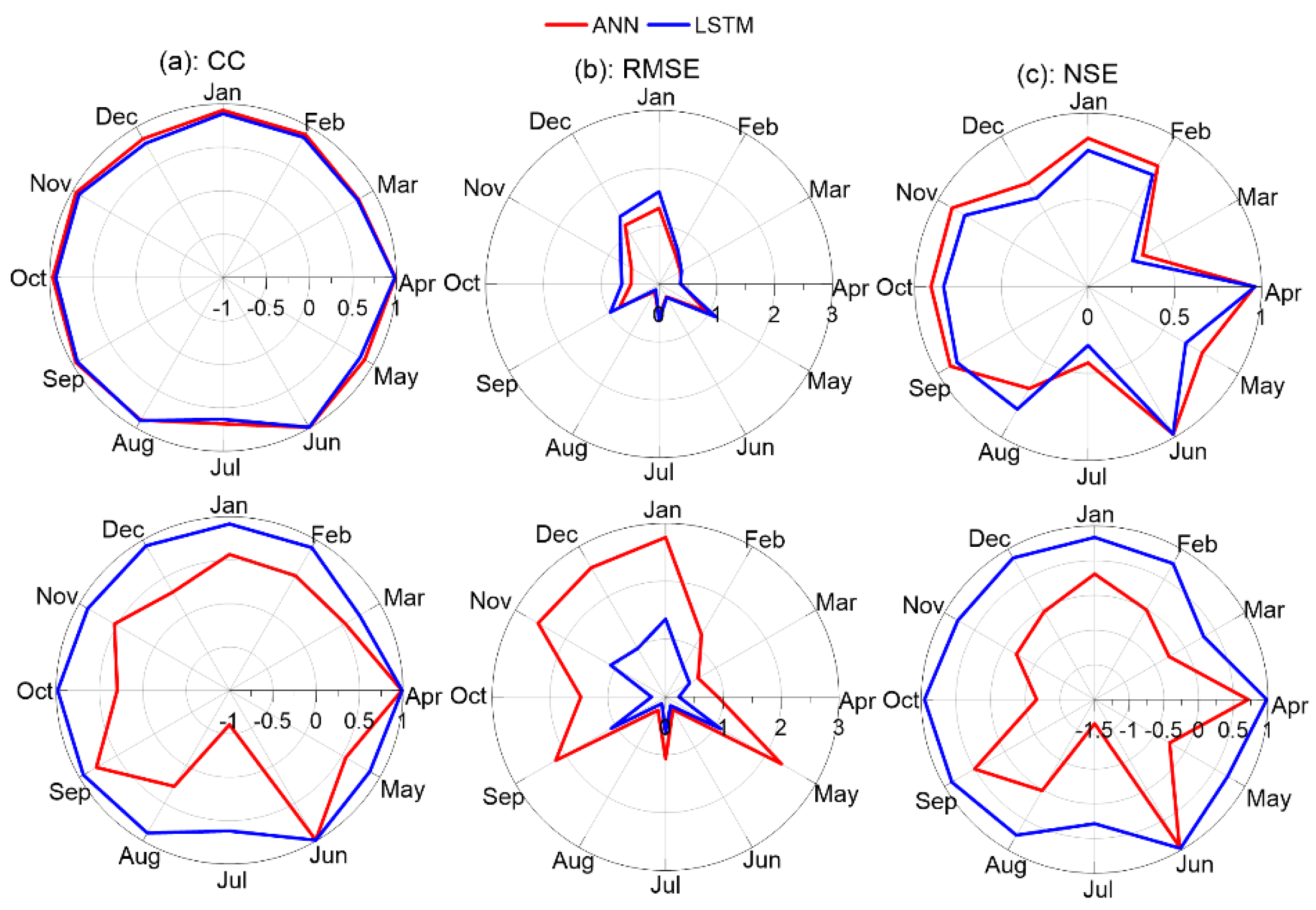
It is very important to understand the prediction performance on a monthly basis, as soil moisture significantly influences flooding and drought. Figure 5 and Figure 6 show the monthly based predictive performance of data-driven models for soil moisture prediction with a lead time of 1 and 6 days for layers 1 and 4. Because the evaluation results of layers 2 and 3 were not significantly different from the results of layers 1 and 4, the evaluation results for each top and deep layer were presented (i.e., layer 1 and layer 4). In the case of layer 1 during the hydrologically wet season (November to March), the evaluation results of the ANN model demonstrate that the average CC was analyzed to be 0.89 and 0.49, RMSE values were 0.81 and 1.95, and NSE values were 0.72 and −0.04 for a lead time of 1 and 6 days. The LSTM model showed better evaluation results, containing 0.85 and 0.87 for CC, 0.99 and 0.90 for RMSE, and 0.65 and 0.71 for NSE. It was found that the ANN model provides slightly better performance for a lead time of 1 day compared to the LSTM model, but the predictive ability decreased as lead time increased.
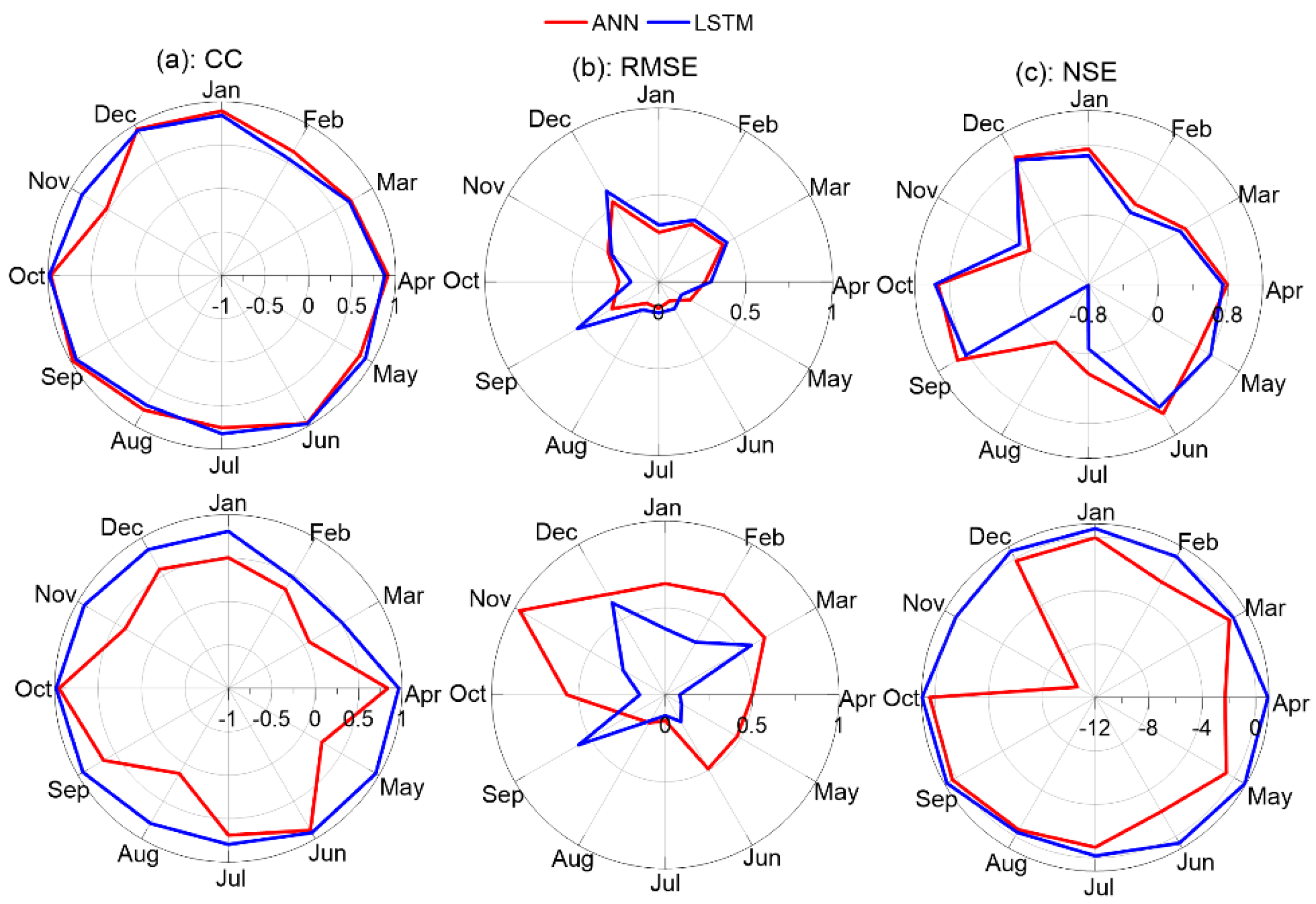
In addition, these models showed sufficient potential for soil moisture prediction during the dry season (April to October) as well as the wet season. Both models provide suitable prediction performance with average CC values of 0.91 and 0.89, RMSE values of 0.51 and 0.59, and NSE values of 0.81 and 0.78 for a lead time of 1 day (Figure 5). As shown in Figure 6, both models provided moderate prediction results, but the ANN model has worse performance for a lead time of 6 days. From the monthly based evaluation results, it was concluded that the data-driven models are sufficient for soil moisture prediction for wet and dry seasons for various soil layers, but it was recommended that the ANN model is suitable for predicting soil moisture for only surface layer than a deep layer, and the LSTM model can provide better soil moisture predictions for both surface and deep layers.
3.3. Errors in Predicted Soil Moisture
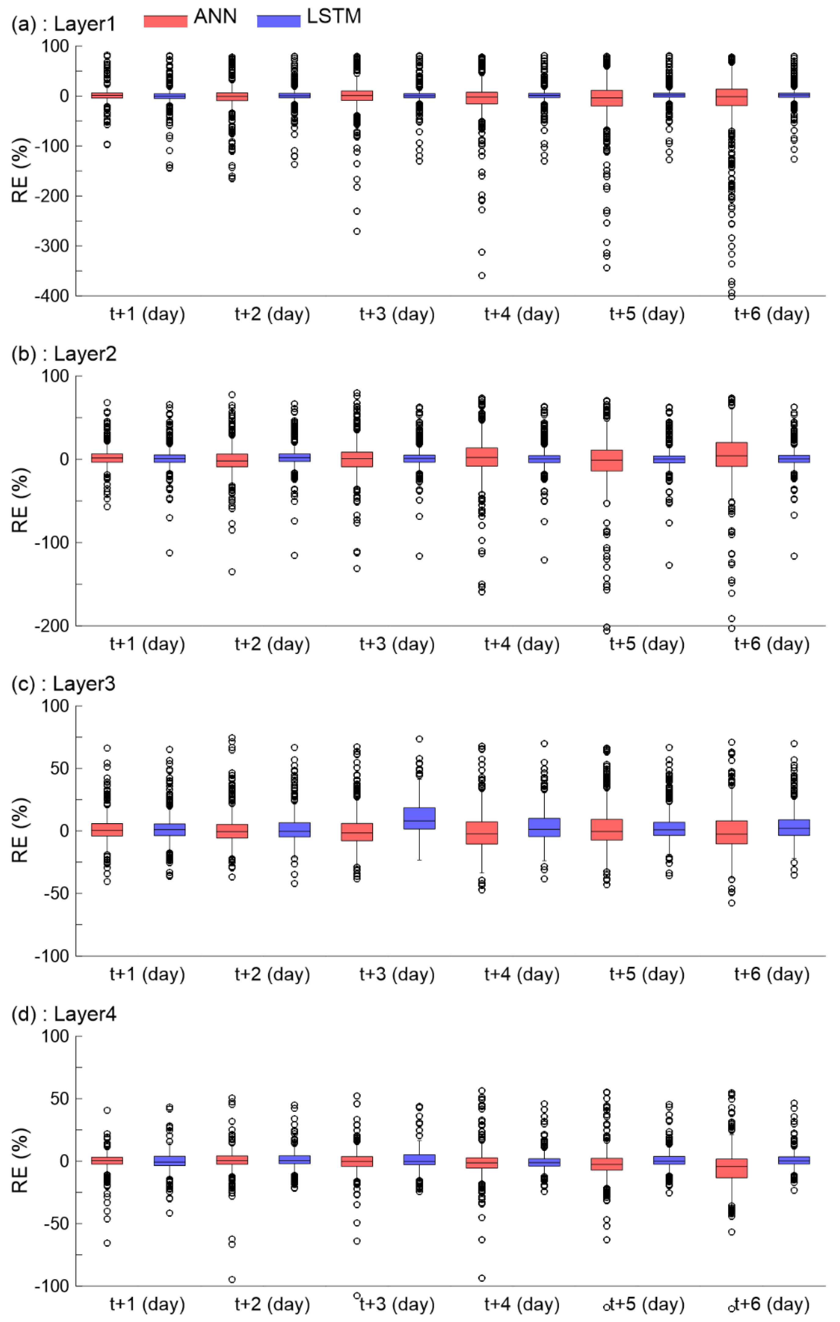
This study investigated how many errors are inherent in the prediction results as the predictive models must be considered according to the characteristics of possible errors for each layer and each lead time. For this, this study used another evaluation metric (i.e., RE (%)) to compare the errors in soil moisture prediction results from ANN and LSTM models. Figure 7 shows box plots representing how much errors are inherent in predicted soil moisture from both models for each layer and lead time from 1 to 6 days.
As shown in Figure 7, it was found that the range of RE values became smaller as the layer became deeper. For example, in layer 1, the maximum RE range was −400% to 100% (lead time of t + 6), whereas in layer 4, it was found to be −100% to 75% (lead time of t + 3 and t + 4). This confirms that the ANN and LSTM models provide a lower prediction error compared to the observation for deep layers, where the temporal variability of soil moisture is relatively small. Moreover, this result shows that the data-driven models have sufficient predictive power for soil moisture prediction for various depths from surface to deep layers. However, comparing the performance of the two models, there was a significant difference in the prediction performance, and the LSTM model clearly demonstrated better prediction results than the ANN model for most of the lead times. ANN model shows better performance for surface layers and short-term prediction. For example, ANN model has better predictive performance for lead time of 1 h and layer 1 (CC = 0.97, RMSE = 0.76, and NSE = 0.94) compared to the LSTM model (CC = 0.96, RMSE = 0.91, and NSE = 0.91). In addition, the ANN model has values of RE ranged from −100% to 80%, whereas the LSTM model has RE values that are ranged from −150% to 80%. Therefore, this study suggested that it is important to select an appropriate model for soil moisture prediction for various depths and lead times.
4. Discussions and Conclusions
In this study, the soil moisture at multiple layers was predicted using meteorological variables with two data-driven models (i.e., ANN and LSTM). This study has the novelty that it provides soil moisture prediction results for multiple layers instead of only a single layer, as shown in other studies. In addition, the prediction results produced from two data-driven models indicated that both models have sufficient potentials for soil moisture analysis as an alternative to the physical-based methods and support to improve the physical-based model’s prediction performance. The results of this study demonstrated that both models showed acceptable prediction results, but the LSTM model showed better predictive performance than the ANN model. More specifically, the LSTM model provided high accurate prediction results with a lead time of 1 to 6 days for four layers. However, the ANN model showed better performance for short-term and surface layers than the LSTM model.
4.1. Limitations of the Data-Driven Models
Although both models showed highly accurate soil prediction results for multiple depths, there are some limitations for the prediction of soil moisture using data-driven models. First, the quality of predicted soil moisture during specific periods showed lower performance compared to the observation. Second, the predicted soil moisture at the third layer showed poor performance than the other three layers.
The main reason for these errors is uncertainties during the training process of the models. The quality and quantity of training data sets affect the performances of the models since the data-driven models predict the time series using the information learned from the data sets [43]. This study used five input data sets to predict the soil moisture for each layer, and if there is uncertainty in only one of them, it can affect the output quality. For example, missing values of observation data affect the training process of the data-driven models and model parameters, which can be transmitted as uncertainty in the validation results. Therefore, it is essential to use quality-proven data sets for model training in order to avoid the malfunction of the data-driven models.
Another reason for the errors in the predicted soil moisture is the uncertainty in the process of driving the models. The data-driven models are called the black-box model because it is difficult for users to capture the uncertainty generated during operating the models. The performances of the data-driven models are significantly influenced by parameters and model structure that are important for training. Inappropriate parameter selection is able to cause overfitting or false-learned issues, which can provide prediction results with lower accuracy. Therefore, it is essential to find optimal values such as dropout rate, various model parameters and use proper equations before the training. Although this study tried to find optimal values of some key parameters and kept them constant after the initial setting, some errors were shown in the predicted soil moisture. The effect of the parameters on model performance is out of the scope of this study, and it will be an important task for future studies.
4.2. Implications for Hydrological Analysis Using Soil Moisture
In this study, two types of data-driven models were applied to predict soil moisture at multiple depths in Eagle Lake point as a case study. The proposed models showed excellent performance, and they can be effective alternatives or supporters of the physical-based model for soil moisture prediction. It was found that the data-driven models can be effective approaches for soil moisture analysis in the area where it is difficult to observe soil moisture directly at various depths due to physical limitations. In addition, it is noteworthy that the data-driven models can collaborate with agricultural, hydrology, and environmental fields that have different purposes of soil moisture usage for each layer. It is expected that the use of the data-driven models will become valuable as the quality of forcing data is improved, and as the technology of computing systems is getting more advanced, the application of complicated data-driven models will be becoming more convenient.
This study suggests that the data-driven models are an effective alternative to the layer-by-layer soil moisture observation method, which has temporal/spatial constraints and is expensive. Moreover, the data-driven models, which have been verified for their reliability in soil moisture prediction, can be used as a reference method for improving the quality of physical models based on complex and diverse equations and methodologies. In this study, a method for predicting the soil moisture value after six days was proposed using meteorological and soil characteristic data. To improve the usability of the predicted results, in future studies, we intend to develop a method for predicting soil moisture for long-term lead time. In addition, based on the results of this study, we intend to develop a complementary method that supplements the weaknesses of both the data-driven models and physical models.
Author Contributions
Conceptualization, H.H., R.R.M., and C.C.; methodology, J.K., H.H. and J.J.; software, C.C. and J.J.; validation, H.H., R.R.M. and H.S.K.; formal analysis, C.C., J.K. and J.J.; investigation, H.H., R.R.M. and H.S.K.; resources, H.S.K.; data curation, C.C. and J.K.; writing—original draft preparation, H.H., J.K. and R.R.M.; writing—review and editing, H.H., R.R.M. and H.S.K.; visualization, H.H. and J.J.; supervision, R.R.M.; project administration, H.S.K.; funding acquisition, H.S.K. All authors have read and agreed to the published version of the manuscript.
Funding
This research was supported by the National Research Foundation of Korea (NRF) grant funded by the Korean government (MSIT) (No. 2017R1A2B3005695).
Conflicts of Interest
The authors declare no conflict of interest.
References
- Islam, S.; Engman, T. Why bother for 0.0001% of Earth’s water? Challenges for soil moisture research. Eos Trans. Am. Geophys. Union 1996, 77, 420. [Google Scholar] [CrossRef]
- Corradini, C.; Morbidelli, R.; Melone, F. On the interaction between infiltration and Hortonian runoff. J. Hydrol. 1998, 204, 52–67. [Google Scholar] [CrossRef]
- Koster, R.D.; Dirmeyer, P.A.; Guo, Z.; Bonan, G.; Chan, E.; Cox, P.; Gordon, C.T.; Kanae, S.; Kowalczyk, E.; Lawrence, D.; et al. Regions of strong coupling between soil moisture and precipitation. Science 2004, 305, 1138–1140. [Google Scholar] [CrossRef] [PubMed] [Green Version]
- Komma, J.; Blöschl, G.; Reszler, C. Soil moisture updating by ensemble Kalman filtering in real-time flood forecasting. J. Hydrol. 2008, 357, 228–242. [Google Scholar] [CrossRef]
- Beck, H.K.; de Jeu, R.A.; Schellekens, J.; van Dijk, A.I.; Bruijnzeel, L.A. Improving curve number based storm runoff estimates using soil moisture proxies. IEEE J. Sel. Top. Appl. Earth Obs. Remote Sens. 2009, 2, 250–259. [Google Scholar] [CrossRef]
- Brocca, L.; Melone, F.; Moramarco, T.; Wagner, W.; Naeimi, V.; Bartalis, Z.; Hasenauer, S. Improving runoff prediction through the assimilation of the ASCAT soil moisture product. Hydrol. Earth Syst. Sci. 2010, 14, 1881–1893. [Google Scholar] [CrossRef] [Green Version]
- Hirschi, M.; Seneviratne, S.I.; Alexandrov, V.; Boberg, F.; Boroneant, C.; Christensen, O.B.; Formayer, H.; Orlowsky, B.; Stepanek, P. Observational evidence for soil-moisture impact on hot extremes in southeastern Europe. Nat. Geosci. 2011, 4, 17–21. [Google Scholar] [CrossRef]
- Li, J.; Islam, S. On the estimation of soil moisture profile and surface fluxes partitioning from sequential assimilation of surface layer soil moisture. J. Hydrol. 1999, 220, 86–103. [Google Scholar] [CrossRef]
- Evans, R.O.; Sneed, R.E. Measuring Soil Water for Irrigation Scheduling: Monitoring Methods and Devices; AG-North Carolina Agricultural Extension Service, North Carolina State University (USA): Raleigh, NC, USA, 1991; Volume 455, 5p. [Google Scholar]
- Ling, P. A review of soil moisture sensors. Assn. Flor. Prof. Bull 2004, 886, 22–23. [Google Scholar] [CrossRef]
- Saxton, K.E.; Johnson, H.P.; Shaw, R.H. Modeling Evapotranspiration and Soil Moisture. Trans. ASAE 1974, 17, 673–677. [Google Scholar] [CrossRef]
- Holtan, H.N. USDAHL-74 Revised Model of Watershed Hydrology; Tech. Bull. 1518; Agricultural Research Service, US Department of Agriculture: Washington, DC, USA, 1975. [Google Scholar]
- Peck, E.L. Catchment Modeling and Initial Parameter Estimation for the National Weather Service River Forecast System; NOAA Technical Memorandum; NWS Hydo-31; National Weather Service: Silver Spring, MD, USA, 1976. [Google Scholar]
- Njoku, E.G.; Jackson, T.J.; Lakshmi, V.; Chan, T.K.; Nghiem, S.V. Soil moisture retrieval from AMSR-E. IEEE Trans. Geosci. Remote Sens. 2003, 41, 215–229. [Google Scholar] [CrossRef]
- Moran, M.S.; Peters-Lidard, C.F.; Watts, J.M.; McElroy, S. Estimating soil moisture at the watershed scale with satellite-based radar and land surface models. Can. J. Remote Sens. 2004, 30, 805–826. [Google Scholar] [CrossRef] [Green Version]
- Wagner, W.; Blöschl, G.; Pampaloni, P.; Calvet, J.C.; Bizzarri, B.; Wigneron, J.P.; Kerr, Y. Operational readiness of microwave remote sensing of soil moisture for hydrologic applications. Hydrol. Res. 2007, 38, 1–20. [Google Scholar] [CrossRef]
- Peng, J.; Loew, A. Recent advances in soil moisture estimation from remote sensing. Water 2017, 9, 530. [Google Scholar] [CrossRef] [Green Version]
- Parinussa, R.M.; Yilmaz, M.T.; Anderson, M.C.; Hain, C.R.; de Jeu, R.A.M. An intercomparison of remotely sensed soil moisture products at various spatial scales over the Iberian Peninsula. Hydrol. Process. 2014, 28, 4865–4876. [Google Scholar] [CrossRef]
- Chauhan, N.S.; Miller, S.; Ardanuy, P. Spaceborne soil moisture estimation at high resolution: A microwave-optical/IR synergistic approach. Int. J. Remote Sens. 2003, 24, 4599–4622. [Google Scholar] [CrossRef]
- Ray, R.L.; Jacobs, J.M.; Cosh, M.H. Landslide susceptibility mapping using downscaled AMSR-E soil moisture: A case study from Cleveland Corral, California, US. Remote Sens. Environ. 2010, 114, 2624–2636. [Google Scholar] [CrossRef]
- Solomatine, D.P.; Ostfeld, A. Data-driven modelling: Some past experiences and new approaches. J. Hydroinf. 2008, 10, 3–22. [Google Scholar] [CrossRef] [Green Version]
- James, T.; Schillaci, C.; Lipani, A. Convolutional neural networks for water segmentation using sentinel-2 red, green, blue (RGB) composites and derived spectral indices. Int. J. Remote Sens. 2021, 42, 5342–5369. [Google Scholar] [CrossRef]
- Kim, S.; Singh, V.P. Modeling daily soil temperature using data-driven models and spatial distribution. Theor. Appl. Climatol. 2014, 118, 465–479. [Google Scholar] [CrossRef]
- Feng, Y.; Cui, N.; Hao, W.; Gao, L.; Gong, D. Estimation of soil temperature from meteorological data using different machine learning models. Geoderma 2019, 338, 67–77. [Google Scholar] [CrossRef]
- Sutskever, I.; Vinyals, O.; Le, Q.V. Sequence to sequence learning with neural networks. Adv. Neural Inf. Process. Syst. 2014, 27, 3104–3112. [Google Scholar]
- Baghdadi, N.; Gaultier, S.; King, C. Retrieving Surface Roughness and Soil Moisture from Synthetic Aperture Radar (SAR) Data Using Neural Networks. Can. J. Remote Sens. 2002, 28, 701–711. [Google Scholar] [CrossRef]
- Zaman, B.; McKee, M.; Neale, C.M. Fusion of remotely sensed data for soil moisture estimation using relevance vector and support vector machines. Int. J. Remote Sens. 2012, 33, 6516–6552. [Google Scholar] [CrossRef]
- Shukla, A.; Panchal, H.; Mishra, M.; Patel, P.R.; Srivastava, H.S.; Patel, P.; Shukla, A.K. Soil moisture estimation using gravimetric technique and FDR probe technique: A comparative analysis. Am. Int. J. Res. Form. Appl. Nat. Sci 2014, 8, 89–92. [Google Scholar]
- Gill, M.K.; Asefa, T.; Kemblowski, M.W.; McKee, M. Soil moisture prediction using support vector machines. JAWRA J. Am. Water Resour. Assoc. 2006, 42, 1033–1046. [Google Scholar] [CrossRef]
- Prakash, S.; Sharma, A.; Sahu, S.S. Soil moisture prediction using machine learning. In Proceedings of the 2018 Second International Conference on Inventive Communication and Computational Technologies (ICICCT), Coimbatore, India, 20–21 April 2018; pp. 1–6. [Google Scholar]
- Achieng, K.O. Modelling of soil moisture retention curve using machine learning techniques: Artificial and deep neural networks vs support vector regression models. Comput. Geosci. 2019, 133, 104320. [Google Scholar] [CrossRef]
- Adeyemi, O.; Grove, I.; Peets, S.; Domun, Y.; Norton, T. Dynamic neural network modelling of soil moisture content for predictive irrigation scheduling. Sensors 2018, 18, 3408. [Google Scholar] [CrossRef] [Green Version]
- Ahmad, S.; Kalra, A.; Stephen, H. Estimating soil moisture using remote sensing data: A machine learning approach. Adv. Water Resour. 2010, 33, 69–80. [Google Scholar] [CrossRef]
- Gorthi, S.; Dou, H. Prediction models for the estimation of soil moisture content. In Proceedings of the ASME 2011 International Design Engineering Technical Conferences and Computers and Information in Engineering Conference, Washington, DC, USA, 28 August 2011; pp. 945–953. [Google Scholar]
- Ali, I.; Greifeneder, F.; Stamenkovic, J.; Neumann, M.; Notarnicola, C. Review of machine learning approaches for biomass and soil moisture retrievals from remote sensing data. Remote Sens. 2015, 7, 16398–16421. [Google Scholar] [CrossRef] [Green Version]
- Efremova, N.; Zausaev, D.; Antipov, G. Prediction of Soil Moisture Content Based on Satellite Data and Sequence-to-Sequence Networks. arXiv 2019, arXiv:1907.03697. [Google Scholar]
- Norbiato, D.; Borga, M.; Degli Esposti, S.; Gaume, E.; Anquetin, S. Flash flood warning based on rainfall thresholds and soil moisture conditions: An assessment for gauged and ungauged basins. J. Hydrol. 2018, 362, 274–290. [Google Scholar] [CrossRef]
- Kim, J.; Han, H.; Kim, B.; Chen, H.; Lee, J. Use of a high-resolution-satellite-based precipitation product in mapping continental-scale rainfall erosivity: A case study of the United States. Catena 2020, 193, 104602. [Google Scholar] [CrossRef]
- Ralph, F.M.; Neiman, P.J.; Wick, G.A.; Gutman, S.I.; Dettinger, M.D.; Cayan, D.R.; White, A.B. Flooding on California’s Russian River: Role of atmospheric rivers. Geophys. Res. Lett. 2006, 33. [Google Scholar] [CrossRef] [Green Version]
- Han, H.; Kim, J.; Chandrasekar, V.; Choi, J.; Lim, S. Modeling Streamflow Enhanced by Precipitation from Atmospheric River Using the NOAA National Water Model: A Case Study of the Russian River Basin for February 2004. Atmosphere 2019, 10, 466. [Google Scholar] [CrossRef] [Green Version]
- Hochreiter, S.; Schmidhuber, J. Long short-term memory. Neural Comput. 1997, 9, 1735–1780. [Google Scholar] [CrossRef]
- Hu, C.; Wu, Q.; Jian, S.; Li, N.; Lou, Z. Deep learning with a long short-term memory networks approach for rainfall-runoff simulation. Water 2018, 10, 1543. [Google Scholar] [CrossRef] [Green Version]
- Fan, H.; Jiang, M.; Xu, L.; Zhu, H.; Cheng, J.; Jiang, J. Comparison of Long Short Term Memory Networks and the Hydrological Model in Runoff Simulation. Water 2020, 12, 175. [Google Scholar] [CrossRef] [Green Version]
- Xiang, Z.; Yan, J.; Demir, I. A rainfall-runoff model with LSTM-based sequence-to-sequence learning. Water Resour. Res. 2020, 56, e2019WR025326. [Google Scholar] [CrossRef]
- Zhang, J.; Zhu, Y.; Zhang, X.; Ye, M.; Yang, J. Developing a Long Short-Term Memory (LSTM) based model for predicting water table depth in agricultural areas. J. Hydrol. 2018, 561, 918–929. [Google Scholar] [CrossRef]
- Tran, Q.K.; Song, S.K. Water level forecasting based on deep learning: A use case of Trinity river-Texas-The United States. J. KIISE 2017, 44, 607–612. [Google Scholar] [CrossRef]
- Lee, G.H.; Jung, S.H.; Lee, D.E. Comparison of physics-based and data-driven models for streamflow simulation of the Mekong river. J. Kor. Water Resour. Assoc. 2018, 51, 503–514. [Google Scholar] [CrossRef]
- Tanty, R.; Desmukh, T.S. Application of artificial neural network in hydrology—A review. Int. J. Eng. Res. Tech. 2015, 4, 184–188. [Google Scholar]
- Jung, J.; Han, H.; Kim, K.; Kim, H.S. Machine Learning-Based Small Hydropower Potential Prediction under Climate Change. Energies 2021, 14, 3643. [Google Scholar] [CrossRef]
- Han, H.; Morrison, R.R. Data-driven approaches for runoff prediction using distributed data. Stoch. Environ. Res. Risk Assess. 2021, 35, 1–19. [Google Scholar] [CrossRef]
Figure 1.
Study area and digital elevation model (DEM). The blue point indicates a SCAN observatory for monitoring various elements.
Figure 1.
Study area and digital elevation model (DEM). The blue point indicates a SCAN observatory for monitoring various elements.

Figure 2.
Conceptual diagram of LSTM model.

Figure 3.
Conceptual diagram of the artificial neural network model [48].
Figure 3.
Conceptual diagram of the artificial neural network model [48].

Figure 4.
Comparison of predicted soil moisture with observations for the four layers ((a): Layer 1, (b): Layer 2, (c): Layer 3, (d): Layer 4) using two data-driven models.
Figure 4.
Comparison of predicted soil moisture with observations for the four layers ((a): Layer 1, (b): Layer 2, (c): Layer 3, (d): Layer 4) using two data-driven models.

Figure 5.
Monthly evaluation results. (a–c) show the statistical metrics (CC, RMSE, and NSE). for layer 1. The first and second lows represent monthly evaluation results for lead times of 1 and 6 days of lead times.
Figure 5.
Monthly evaluation results. (a–c) show the statistical metrics (CC, RMSE, and NSE). for layer 1. The first and second lows represent monthly evaluation results for lead times of 1 and 6 days of lead times.

Figure 6.
Monthly evaluation results. (a–c) show the statistical metrics (CC, RMSE, and NSE) for layer 4. The first and second lows represent monthly evaluation results for lead times of 1 and 6 days of lead times.
Figure 6.
Monthly evaluation results. (a–c) show the statistical metrics (CC, RMSE, and NSE) for layer 4. The first and second lows represent monthly evaluation results for lead times of 1 and 6 days of lead times.

Figure 7.
Box plots representing relative error (RE, %) of predicted soil moisture from both models for four layers ((a): Layer 1, (b): Layer 2, (c): Layer 3, (d): Layer 4). The red box represents ANN, and the blue is LSTM results.
Figure 7.
Box plots representing relative error (RE, %) of predicted soil moisture from both models for four layers ((a): Layer 1, (b): Layer 2, (c): Layer 3, (d): Layer 4). The red box represents ANN, and the blue is LSTM results.


Table 1.
Evaluation results obtained by statistical metrics for estimated soil moistures from the two models.
Table 1.
Evaluation results obtained by statistical metrics for estimated soil moistures from the two models.
| Layers | Lead Time (days) | ANN | LSTM | ||||
|---|---|---|---|---|---|---|---|
| CC | RMSE | NSE | CC | RMSE | NSE | ||
| 1 | 1 | 0.97 | 0.76 | 0.94 | 0.96 | 0.91 | 0.91 |
| 2 | 0.93 | 1.10 | 0.87 | 0.96 | 0.88 | 0.92 | |
| 3 | 0.89 | 1.42 | 0.78 | 0.96 | 0.88 | 0.92 | |
| 4 | 0.86 | 1.59 | 0.73 | 0.96 | 0.87 | 0.92 | |
| 5 | 0.82 | 1.78 | 0.66 | 0.96 | 0.84 | 0.92 | |
| 6 | 0.80 | 1.89 | 0.62 | 0.96 | 0.84 | 0.93 | |
| 2 | 1 | 0.97 | 0.68 | 0.93 | 0.96 | 0.75 | 0.91 |
| 2 | 0.93 | 0.96 | 0.86 | 0.95 | 0.79 | 0.90 | |
| 3 | 0.89 | 1.19 | 0.78 | 0.96 | 0.76 | 0.91 | |
| 4 | 0.85 | 1.35 | 0.71 | 0.95 | 0.76 | 0.91 | |
| 5 | 0.83 | 1.42 | 0.68 | 0.95 | 0.78 | 0.90 | |
| 6 | 0.82 | 1.51 | 0.64 | 0.96 | 0.75 | 0.91 | |
| 3 | 1 | 0.93 | 0.51 | 0.85 | 0.91 | 0.58 | 0.81 |
| 2 | 0.87 | 0.65 | 0.75 | 0.90 | 0.58 | 0.80 | |
| 3 | 0.85 | 0.68 | 0.73 | 0.90 | 0.66 | 0.74 | |
| 4 | 0.85 | 0.70 | 0.72 | 0.90 | 0.58 | 0.80 | |
| 5 | 0.83 | 0.74 | 0.67 | 0.90 | 0.58 | 0.80 | |
| 6 | 0.80 | 0.79 | 0.63 | 0.90 | 0.59 | 0.80 | |
| 4 | 1 | 0.98 | 0.32 | 0.97 | 0.98 | 0.36 | 0.96 |
| 2 | 0.97 | 0.45 | 0.93 | 0.98 | 0.36 | 0.96 | |
| 3 | 0.95 | 0.53 | 0.90 | 0.98 | 0.38 | 0.95 | |
| 4 | 0.94 | 0.60 | 0.88 | 0.98 | 0.37 | 0.95 | |
| 5 | 0.93 | 0.63 | 0.87 | 0.98 | 0.38 | 0.95 | |
| 6 | 0.91 | 0.74 | 0.82 | 0.98 | 0.37 | 0.95 | |
Publisher’s Note: MDPI stays neutral with regard to jurisdictional claims in published maps and institutional affiliations. |
© 2021 by the authors. Licensee MDPI, Basel, Switzerland. This article is an open access article distributed under the terms and conditions of the Creative Commons Attribution (CC BY) license (https://creativecommons.org/licenses/by/4.0/).
Share and Cite
MDPI and ACS Style
Han, H.; Choi, C.; Kim, J.; Morrison, R.R.; Jung, J.; Kim, H.S. Multiple-Depth Soil Moisture Estimates Using Artificial Neural Network and Long Short-Term Memory Models. Water 2021, 13, 2584. https://doi.org/10.3390/w13182584
AMA Style
Han H, Choi C, Kim J, Morrison RR, Jung J, Kim HS. Multiple-Depth Soil Moisture Estimates Using Artificial Neural Network and Long Short-Term Memory Models. Water. 2021; 13(18):2584. https://doi.org/10.3390/w13182584
Chicago/Turabian StyleHan, Heechan, Changhyun Choi, Jongsung Kim, Ryan R. Morrison, Jaewon Jung, and Hung Soo Kim. 2021. "Multiple-Depth Soil Moisture Estimates Using Artificial Neural Network and Long Short-Term Memory Models" Water 13, no. 18: 2584. https://doi.org/10.3390/w13182584
Note that from the first issue of 2016, this journal uses article numbers instead of page numbers. See further details here.