
Environmental Flows as a Proactive Tool to Mitigate the Impacts of Climate Warming on Freshwater Macroinvertebrates


1
Hellenic Centre for Marine Research, Institute of Marine Biological Resources & Inland Waters, 46.7 km Athens-Sounio Ave., 19013 Anavyssos, Greece
2
Department of Water Resources & Environmental Engineering, National Technical University of Athens, 5 Iroon Polytechniou Str., 15780 Athens, Greece
*
Author to whom correspondence should be addressed.
Water 2021, 13(18), 2586; https://doi.org/10.3390/w13182586
Submission received: 30 June 2021
/
Revised: 10 September 2021
/
Accepted: 13 September 2021
/
Published: 18 September 2021
(This article belongs to the Special Issue Emerging Trends in Freshwater Ecology and Ecosystem Management)
Abstract
:What would happen in Mediterranean rivers and streams if warming but not drying occurred? We examined whether the delivery of environmental flows within a warming climate can maintain suitable macroinvertebrate habitats despite warming. A two-dimensional ecohydraulic model was used to (1) simulate the influence of water temperature and flow on macroinvertebrates by calculating habitat suitability for 12 climate change scenarios and (2) identify the mechanism by which macroinvertebrate assemblages respond to warming. The results suggest that not all watersheds will be equally influenced by warming. The impact of warming depends on the habitat conditions before warming occurs. Watersheds can, thus, be categorized as losing (those in which warming will degrade current optimal thermal habitat conditions) and winning ones (those in which warming will optimize current sub-optimal thermal habitat conditions, until a given thermal limit). Our models indicate that in losing watersheds, the delivery of environmental flows can maintain suitable habitats (and, thus, healthy macroinvertebrate assemblages) for up to 1.8–2.5 °C of warming. In winning watersheds, environmental flows can maintain suitable habitats when thermal conditions are optimal. Environmental flows could, thus, be used as a proactive strategy/tool to mitigate the ecological impacts of warming before more expensive reactive measures within a changing climate become necessary.
1. Introduction
Since the 1940s, and mostly since the 1980s, the Earth’s natural cooling–warming cycle has been interrupted by specific, rapidly expanding human activities, outcompeting natural processes. Agro-industrial and residential carbon dioxide (CO2) and methane (CH4) emissions have been strongly associated with a post-1980 steep increase in the global average air temperature [1,2]. Eventually, this global temperature rise—expected to increase by 3–5 °C by 2100, compared to the early 2000s [2]—has already caused, and it is expected to intensify, a global climate change that has resulted, inter alia, in more frequent and extreme local floods and droughts [3]. In Mediterranean climate areas, warming has already led to higher rates of evaporation and lower levels of precipitation, resulting in decreased river flows and lake water levels [4,5,6]. It is projected that Mediterranean climate river waters will warm by 0.5–4 °C and river flows will decline by 34% by 2071–2100 [7,8].
Thus, global warming causes varying and often contrasting local hydrological responses [4,9]. For example, river flows in northern Europe, northern Asia and high-latitude North America are projected to increase by 10–40% by 2050, but in southern Africa, southern Europe, the Middle East and mid-latitude western North America, they are expected to decline by 10–30% [4]. These warming-induced hydroclimatic changes have already changed the structure and functioning of Mediterranean freshwater ecosystems, but ecosystem response to climate change also varies across regions [9]. Macroinvertebrate assemblages in warming waters have been characterized by lower density [10], biodiversity and taxonomic richness [11] compared to colder waters, but elsewhere, overall assemblage abundance and richness did not change [12] or even increase [13,14]. As a result, there are (and will further be) winners and losers across regions within continents, and across watersheds within regions, both from a hydrological (discharge may increase in some regions (winners) and decrease in others (losers)) and from an ecological perspective (density, biodiversity and richness may increase in some regions (winners) and decrease in others (losers)).
While most studies have focused on assessing the hydro-ecological impacts of climate change, few studies have explored the effects of proactive climate change mitigation practices on freshwater ecosystems. Theoretically, mitigation tools, and associated practices, exist but environmental flows are rarely explored as one of them [15,16]. Forslund et al. [15], based on a study in the central and lower Yangtze River, concluded that “securing environmental flows builds the capacity of the ecosystem to better adapt to impacts from climate change”. This has been further supported for benthic macroinvertebrates by Theodoropoulos et al. [16], who concluded that environmental flows could partially counterbalance macroinvertebrate habitat loss due to warming, compensating benthic assemblages for up to 3–5 °C of warming if near-natural flows are maintained in Mediterranean rivers. However, relevant studies to further support or apply (or even possibly disprove) this concept (the concept that environmental flows could increase the resistance and resilience of aquatic ecosystems to warming) are rare.
The aim of this study was to examine if the delivery and maintenance of environmental flows in Mediterranean streams within a warming aquatic environment (due to climate change) are capable of maintaining suitable macroinvertebrate habitats (and thus, healthy benthic assemblages) despite warming. Using 365 macroinvertebrate samples from Greece, we quantified the influence of water temperature on macroinvertebrate habitat suitability (HSI) and simulated HSI changes in varying warming scenarios (from 0 to +5 °C) and flow conditions (from natural and near-natural to environmental and near-dry flows), in two river reaches in Greece. Our purpose was not only to examine whether or not environmental flows can be used as a proactive climate change mitigation tool, but also to quantify, for each warming scenario, the flow requirements of benthic macroinvertebrates that are necessary to maintain suitable habitats (and, thus, their assemblage structure unchanged) despite warming. To clarify and further elaborate, we know that in Mediterranean climates, global warming has and will further cause local drying, forcing aquatic ecosystems to eventually adapt [7,8]; but what would happen if rivers kept flowing despite the increased water temperatures? We suggest that if macroinvertebrate habitats remained healthy and able to sustain healthy macroinvertebrate communities, it would be worth researching and funding proactive practices/strategies of delivering environmental flows to rivers to keep their ecosystem habitats healthy and maintain the valuable services they provide to societies, despite the inevitable warming.
2. Materials and Methods
2.1. Case Studies
The effects of climate warming on macroinvertebrate habitat suitability were explored in two study areas in Greece: (1) the Evrotas River and (2) the Oenoe Stream. The Evrotas River reach is 443 m long (catchment area: 10,227 m2), located in southern Peloponnese, at an elevation of 227 m a.s.l. The Oenoe Stream reach is 370 m long (catchment area: 3731 m2), located in Attica, downstream of the Marathon Reservoir, at an elevation of 102 m a.s.l. (Figure 1). Both areas have a temperate Mediterranean climate characterized by mild winters and hot, prolonged dry summers. Air temperature mostly varies between 5 °C and 29 °C, often reaching below 0 °C and above 33 °C. Average annual precipitation is low, compared to that of the western and northern parts of the Greek territory. July, August and September are the driest months of the year. Both areas are surrounded by forests and shrubs, which have been gradually replaced mostly by agricultural and less by urban areas.
2.2. Climatic Data and Climate Change Scenarios
First, we calculated the average annual water discharge (Q) and the average annual water temperature (TW) for each study reach based on historical hydro-climatic data assembled from (i) https://www.meteoblue.com (accessed on 18 September 2021) (30-year simulated air temperatures) and (ii) seasonal TW and Q records of the Greek Surface Water Monitoring Programme from 2012 to 2020. Then, we simulated the hydraulic properties (flow velocity and water depth distribution) and macroinvertebrate habitat suitability at each river reach for 12 primary climate change scenarios (Table 1) and for 18 additional Q-TW scenarios, corresponding to all Q and TW combinations for a Q change of 0%, 25%, 50%, 75%, 90% and 99%, and TW change of 0 °C, 1.6–1.8 °C, 2–2.5 °C, 3 °C and 5 °C from the current average. Six of the 12 primary scenarios were based on the standard Special Report on Emissions Scenarios projected for the 2071–2100 period by the Intergovernmental Panel on Climate Change (SRES A2 and SRES B1) [17], adapted for freshwaters by [7] using three general circulation models (CNCM3, ECHAM, IPSL). The other six primary scenarios were extreme-case, study-specific scenarios (Q change ≥ 90%; TW change ≥ 2–2.5 °C).
The annual average Q and TW for the Evrotas River were 2.5 m3/s and 15.46 °C, respectively, based on 2-year and 4-year hydro-climatic datasets (daily observations from 2010 to 2011 for Q, and from 2016 to 2020 for TW). The annual average Q and TW for the Oenoe Stream were 0.6 m3/s and 16.46 °C, respectively, based on 11-year and 8-year hydro-climatic datasets (daily observations from 2003 to 2013 for Q, and from 2010 to 2018 for TW).
2.3. Hydraulic Models
Hydraulic simulations have been previously applied in both study reaches to calculate environmental flows [18,19] The topography of each reach was mapped with topographic points recording longitude, latitude and altitude using a real-time kinematic (RTK) GPS (Spectra Precision SP60 GNSS Receiver + MobileMapper 10 GIS-GPS Receiver; Trimble Inc., California, CA, USA). A total of 719 coordinate points were recorded for the 443 m long Evrotas River reach, and 459 points were recorded for the 370-meter-long Oenoe Stream reach. Data were processed in Blue KenueTM 64 v3.3 (NRCC, Canada). An unstructured, triangular computational mesh was developed for each study reach (Oenoe Stream reach: 3938 nodes, 7140 elements; Evrotas River reach: 13,477 nodes, 25,998 elements), and boundary and initial conditions were defined for each climate change scenario. Q was prescribed at the upstream boundary and the water surface elevation was prescribed at the downstream boundary based on relevant stage–discharge curves. The TELEMAC-2D v6.2 hydrodynamic model [20] was used to calculate water depths (D) and depth-averaged flow velocities (V) in various discharges. Three hydrometric surveys were carried out (in three different discharges: 0.008 m3/s, 0.02 m3/s and 0.5 m3/s) in the Evrotas River reach to calibrate and validate the hydraulic simulations. Two hydrometric surveys were carried out in the Oenoe Stream reach (0.03 m3/s and 0.3 m3/s). At each survey, flow velocity (V) and water depth (D) were measured at 15–20 randomly selected points across each reach. For the Evrotas River reach, simulations were calibrated using the V and D values from the 0.02 m3/s hydrometric survey and validated using the V and D values from the other two surveys. For the Oenoe Stream reach, simulations were calibrated using the V and D values from the 0.03 m3/s hydrometric survey and validated using the V and D values of the 0.3 m3/s survey. Both models were calibrated–validated by adjusting the Manning’s roughness coefficient at different sections of each study reach, based on an on-site visual assessment of the substrate types (S), until acceptable R2 values between calculated and observed V and D were achieved. The validated models were used to calculate V and D for all discharges included in the 12 climate change scenarios + the current “reference” discharge (in total: (5 + 1) discharges × 2 study areas = 12 hydraulic simulations).
2.4. Habitat Suitability Curves and Habitat Suitability Models
Macroinvertebrate habitat preferences for V, D, S and TW were acquired from the benthos-GR dataset [21], consisting of 380 microhabitat observations relating V, D, S and TW with the habitat suitability of macroinvertebrates (HSI; totally unsuitable: 0, totally suitable: 1) using an assemblage-based index that combines taxonomic richness, diversity (Shannon’s index), Ephemeroptera–Plecoptera–Trichoptera (EPT) richness and total assemblage abundance [22]. Macroinvertebrates were sampled from a maximum of 20 rectangular microhabitats delineated as combinations of V, D and S at nine sites in Greece, in three seasons (spring, summer, autumn). A 0.25 × 0.25 m2 Surber sampler with a mesh size of 500 μm was used, resulting in a total sampling area of 0.0625 m2 at each microhabitat. Macroinvertebrates were sorted and identified to the family level using a stereo microscope. HSI–TW relationships were identified by developing generalized linear mixed-effects models (GLMMs) in R version 3.5.1 [23]. GLMMs were fitted using the gamlss package v5.3-4 [24]. The logspline package v2.1.16 [25] was employed to find the distribution that best fitted our response variable (HSI). TW was used as a fixed factor. Flow velocity, water depth, the type of substrate, sampling season, river basin and site were used as random factors to account for spatial and temporal autocorrelation. We applied both linear and cubic-splines-based models and selected the model that best fitted our data based on the lowest AIC and highest R2 coefficient (Cox–Snell presudo-R2 using the rsq package v2.2 [26]).
Using the benthos–GR dataset as a reference/training dataset, macroinvertebrate habitat suitability at each node of the computational mesh for each Q and TW scenario was calculated using a fuzzy rule-based Bayesian algorithm (FRB), implemented in the HABFUZZ v2.8.1 software [27]. For each node of the computational mesh, (1) the numerical outputs of the hydraulic simulations (the V and D values calculated), (2) the node’s S and (3) the reach’s TW (based on the scenarios of Table 1) were used as inputs to the FRB habitat model and converted to overlapping, trapezoidal-shaped, membership functions (fuzzy sets) [21,28]. Thus, each numerical input was assigned to one or more fuzzy sets with a membership degree (MD) ranging from zero to one; HSI values were also categorized in five classes (0 ≤ bad ≤ 0.2; 0.2 < poor ≤ 0.4; 0.4 < moderate ≤ 0.6; 0.6 < good ≤ 0.8; 0.8 < high ≤ 1). Based on the training dataset, IF–THEN rules, relating the input fuzzy sets with a specific HSI class were developed. The fuzzy MD of each input variable (V, D, S and TW) was considered as the probability of occurrence of the particular fuzzy set, such as “IF V is low with a membership degree of 1 AND D is moderate with a MD of 1 AND S is gravel with a MD of 1 THEN HSI is high with an MD of 0.3 and good with a MD of 0.7”. The IF–THEN rules were then combined using the Bayesian joint probability, so that (referring to the previous example) the probability of the specific node’s being high is the joint probability that V is low AND D is moderate AND S is gravel AND HSI is high (1 × 1 × 1 × 0.3 = 0.3), while the probability of HSI being good is the joint probability that V is low AND D is moderate AND S is gravel AND HSI is good (1 × 1 × 1 × 0.7 = 0.7). A score was assigned to each HSI class (bad: 0.1, poor: 0.3, moderate: 0.5, good: 0.7, high: 0.9) and the habitat suitability for each node of the mesh was predicted as , where HSI is the calculated habitat suitability, Mij denotes the joint probability of occurrence of each HSI class, and Sij denotes the score of each HSI class. For the previous example, HSI equals to 0.7 × 0.7 + 0.3 × 0.9 = 0.76 (good).
Based on the climate change scenarios of Table 1, and the additional scenarios, we developed a test dataset for each scenario by appropriately changing the V and D (calculated for each Q from the hydraulic simulations) and the TW values accordingly. In total, 12 test datasets were developed for each study reach, corresponding to the 12 primary climate change scenarios, and 18 test datasets were additionally developed for each study reach, corresponding to all other Q and TW combinations (in total: (12 + 18) scenarios × 2 study reaches = 60 habitat simulations).
2.5. Reach-Scale Habitat Suitability and Comparisons between Scenarios
Based on the HSI, we calculated a reach-scale suitability index (HSIR) as follows: , where is the mean HSI of all mesh nodes, w is the number of wetted (not dry) nodes of the reach, and C is the ratio of connected (neighboring) nodes with HSI > 0.6 to the total number of wetted nodes with HSI > 0.6. HSI and HSIR values > 0.6 were considered suitable, and all comparisons between the 12 + 18 climate change scenarios were based on the values of the node-scale HSI and the reach-scale HSIR suitability indices. To ease comparisons among climate change scenarios, each scenario is expressed as “the Q|Tw scenario”. For example, the SRES B1/CNCM3 scenario, with a 25–50% Q change from current average and a 1.6–1.8 °C TW change from current average, is written as “the 50%|1.6–1.8 scenario”. To identify potential macroinvertebrate assemblage differences between groups of sites, permutational analysis of variance (PERMANOVA) was applied in the PRIMER 6+ Software v6.1.13 (PRIMER-e, Auckland, New Zealand).
3. Results
3.1. Water Temperature and Macroinvertebrate Habitat Suitability
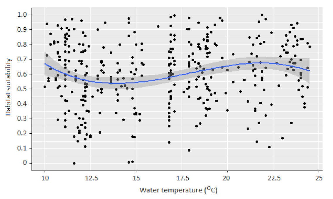
Water temperature in the 380-microhabitat dataset ranged from 10 to 24.5 °C (mean: 16.41 °C; SD: 4.33) and significantly influenced the habitat suitability of macroinvertebrates (p = 0.00014). The relationship between TW and HSI was best modelled (using cubic-splines-based generalized linear mixed-effects models) by a sine-shaped habitat suitability curve (R2 = 0.42) (Figure 2). This best-fit curve starts with a peak HSI (0.67) at the lowest TW (10 °C), declines until TW = 14 °C, increases after 14 °C and peaks again at approx. 22 °C, further declining to HSI < 0.6 until 24.5 °C.
3.2. Case Study I: The Oenoe Stream (a Losing Watershed)
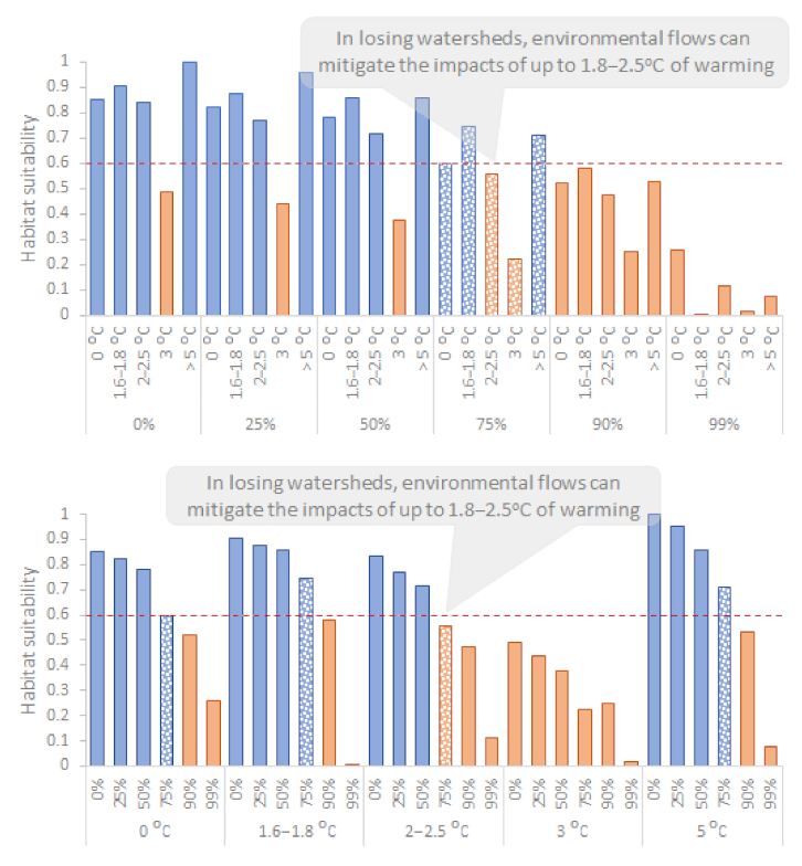
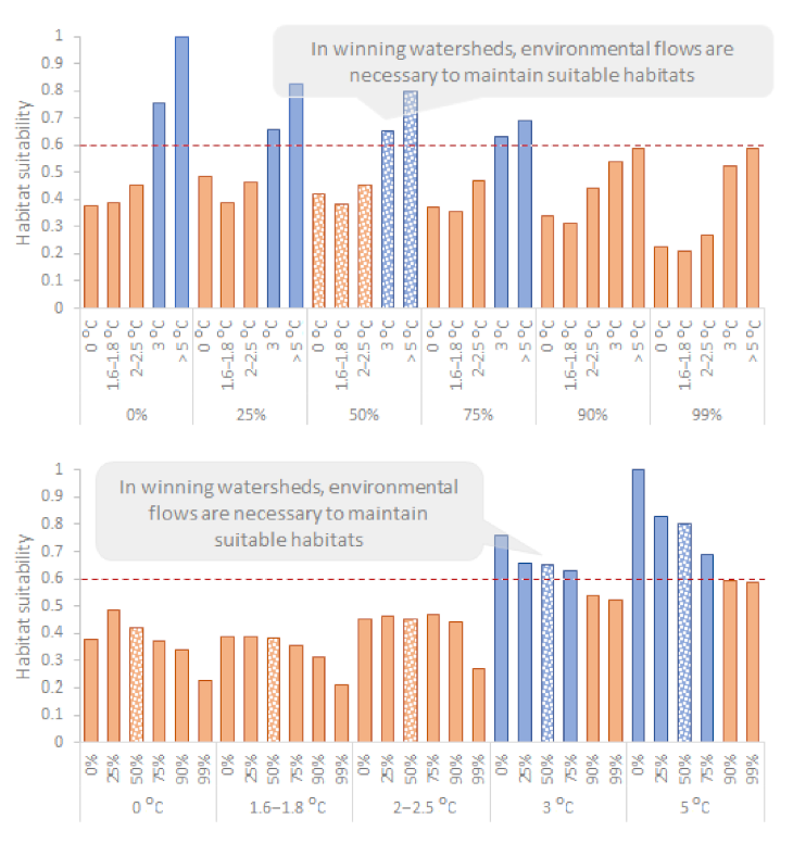
The reference annual average Q in the Oenoe Stream was 0.61 m3/s and the reference annual average TW was 16.46 °C. Within the various IPCC-based and extreme climate warming scenarios simulated, the following patterns were observed (Figure 3): (1) Overall, TW-HSIR relationships followed the sine-shaped habitat suitability curve, with HSIR peaking at low TW values (0 °C to +1.6–1.8 °C TW change), decreasing as TW increased (+1.6–1.8 °C, +2–2.5 °C, +3 °C) and increasing again as warming reached +5 °C, following the second peak of the sine-shaped curve. (2) Regardless of Q change, HSIR was unsuitable (<0.6) for all +3 °C scenarios. (3) Regardless of TW change, HSIR was unsuitable for all Q > 90% and Q > 99% change scenarios. (4) For up to 75% of Q decrease from current average (corresponding to the environmental flow for this study reach), HSIR was suitable (>0.6) for a TW increase of up to 1.8 °C and slightly below 0.6 for a 2.5 °C TW increase from the current average.
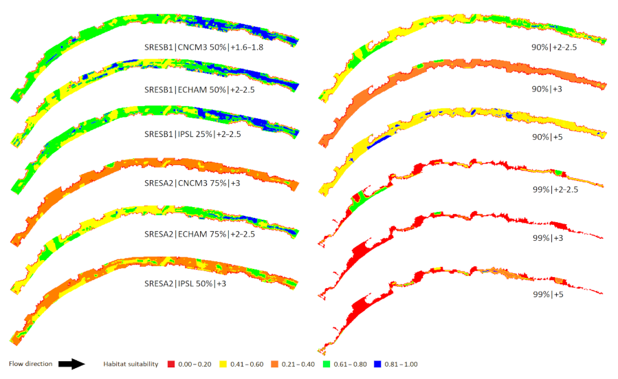
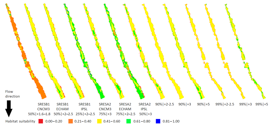
Three of the six IPCC scenarios (SRES B1/CNCM3: Q = −50%, TW = +1.6–1.8 °C; SRES B1/IPSL: Q = −25%, TW = +2–2.5 °C; SRES B1/ECHAM: Q = −50%, TW = +2–2.5 °C) (50%) were mostly suitable for macroinvertebrates (Figure 4), with HSIR = 0.86, 0.77 and 0.72, respectively. For 2/6 scenarios (SRES A2/CNCM3: Q = −75%, TW = +3 °C; SRES A2/IPSL: Q = −50%, TW = +3 °C) (33%), most microhabitats across the reach were unsuitable for macroinvertebrates, with HSIR = 0.22 and 0.38, respectively. For 1/6 scenarios (SRES A2/ECHAM: Q = −75%, TW = +2–2.5 °C) (17%), the share between suitable and unsuitable microhabitats was almost equal (the upstream half being mostly unsuitable; the downstream half being mostly suitable). All extreme drying scenarios (Q change > 90%) resulted in unsuitable macroinvertebrate habitats, with the lowest suitability for Q > 99% change scenarios.
3.3. Case Study II: The Evrotas River (a Winning Watershed)
The reference annual average Q in the Evrotas River was 2.5 m3/s, and the reference annual average TW was 15.46 °C. Within the various IPCC-based and extreme climate warming scenarios simulated, the following patterns were observed (Figure 5): (1) Overall, TW-HSIR relationships partially followed the sine-shaped habitat suitability curve, with HSIR being low at lowest TW values (corresponding to the current TW average), slightly decreasing at TW = +1.6–1.8 °C and increasing again as TW further increased, peaking only at the highest TW values (+3 °C and +5 °C TW change). (2) Regardless of Q change, HSIR was unsuitable (<0.6) for all +0 °C, +1.6–1.8 °C and +2–2.5 °C change scenarios. (3) Regardless of TW change, HSIR was unsuitable for all Q > 90% and Q > 99% scenarios. (4) HSIR was suitable only for high TW values (+3 °C and +5 °C TW change), as long as Q change is ≤75% (slightly lower than the environmental flow of the study reach).
Two of the six IPCC scenarios (SRES A2/CNCM3: Q = −75%, TW = +3 °C; SRES A2/IPSL: Q = −50%, TW = +3 °C) (33%) were suitable for macroinvertebrates (although with extended unsuitable areas) (Figure 6), with HSIR = 0.63 and 0.65, respectively. For 4/6 scenarios (SRES B1/CNCM3: Q = −50%, TW = +1.6–1.8 °C; SRES B1/IPSL: Q = −25%, TW = +2–2.5 °C; SRES B1/ECHAM: Q = −50%, TW = +2–2.5 °C; SRES A2/ECHAM: Q = −75%, TW = +2–2.5 °C) (67%), most microhabitats across the reach were unsuitable for macroinvertebrates, with HSIR = 0.38, 0.46, 0.45 and 0.47, respectively. All extreme drying scenarios (Q change > 90%) resulted in unsuitable macroinvertebrate habitats regardless of TW.
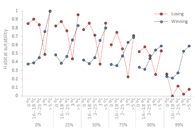
3.4. Losing vs. Winning Watersheds
The Oenoe Stream is a losing watershed; habitat suitability in current TW and Q conditions (reference scenario; 0 °C change) is high and decreases as TW increases (although suddenly peaking when TW change exceeds 5 °C; see the discussion for a possible explanation) (Figure 3 and Figure 7). In contrast, the Evrotas River is a winning watershed; habitat suitability in current TW and Q conditions is low and increases as TW increases, peaking at TW change > 5 °C (Figure 5 and Figure 7). These winning or losing TW–HSIR trends are repeated in all Q scenarios for both areas/watersheds but successively decline as Q decreases from the current average.
4. Discussion
The results of the study indicate an interactive influence of water temperature and flow on the habitat suitability of benthic macroinvertebrates. At near-dry flows (>90% discharge decrease from current average), flow is the major determinant of macroinvertebrate habitat suitability (our models showed habitat suitability <0.6 for all warming scenarios at discharge change >90%). For discharges up to 50–75% decreased from the current average, water temperature is the major determinant of macroinvertebrate habitat suitability. It seems that the mechanism, based on which habitat suitability is shaped by water temperature in these flows (natural, near-natural, intermediate and environmental flows), depends on the current (reference) average water temperature (i.e., the average thermal conditions in the river at the time that warming begins). As such, watersheds can be categorized in (1) winning watersheds: those in which current thermal conditions are sub-optimal for macroinvertebrates, and thus, climate warming will likely lead to optimizing macroinvertebrate habitats and habitat suitability, and (2) losing watersheds: those in which current thermal conditions are optimal for macroinvertebrates, and thus, warming will likely lead to sub-optimal, unsuitable habitats and habitat suitability. In our study, the Evrotas River reach is a winning watershed, and the Oenoe Stream reach is a losing one. This could be possibly due to the different altitudes of each study reach that resulted in different “initial” thermal conditions, but latitude could also be a second variable shaping different “initial” thermal conditions upon which climate warming will act.
4.1. In Losing Watersheds, Environmental Flows Can Mitigate the Impacts of up to 1.8–2.5 °C of Warming
In our losing watershed (the Oenoe Stream reach), maintenance of natural flows (0% decrease from current average), near-natural (−25%) and intermediate flows (−50%) resulted in acceptable habitat suitability for up to 2.5 °C of warming. Environmental flows (−75% from current average) also shaped suitable habitats for up to 1.8 °C of warming, marginally unacceptable (HSIR = 0.55) at 2–2.5 °C. When warming exceeded 2.5 °C, habitat suitability was low/unacceptable in all discharges simulated, increasing again as warming increased to +5 °C. Thus, our models indicate that (1) when current thermal conditions are optimal for macroinvertebrates (a losing watershed), warming will reduce habitat suitability, but the delivery of natural or near-natural flows could maintain suitable habitats for up to 2–2.5 °C of warming. The delivery of environmental flows could maintain suitable habitats for up to 1.8 °C of warming. (2) When warming exceeds 3 °C, our data indicate that existing macroinvertebrate assemblages decline, cold-dwelling and/or thermo-sensitive taxa are replaced by thermo-tolerant ones and assemblages are forced to adapt to warmer conditions. In our case (in the 380-microhabitat dataset), thermo-sensitive taxa within families of Chironomidae [29], Baetidae [30], Heptageniidae [31] and Ephemerellidae [32] were probably gradually replaced by thermo-tolerant taxa of Caenidae [33], Gomphidae [34], Hydropsychidae, Elmidae, Hydraenidae [35] and Leuctridae (Appendix, Table A1); the latter being the only taxonomic group that does not fully support our interpretation (Leuctridae have long been considered thermo-sensitive, with the optimal water temperature at 14 °C [36]; however, they also occur in warmer waters [37,38])—it must be noted that not all genera and/or species within a family are thermo-tolerant or thermo-sensitive. At 5 °C of warming, thermo-tolerant taxa are well established, habitat suitability increases again to acceptable levels but this is probably due to a new macroinvertebrate assemblage that has eventually been established (assemblage structure at <2–2.5 °C was statistically different from that at +5 °C of warming; PERMANOVA t = 4.175; p < 0.001).
4.2. In Winning Watersheds, Environmental Flows Are Necessary to Maintain Suitable Habitats
In our winning watershed (the Evrotas River reach), water temperature was the main habitat suitability determinant, and flow did not significantly affect habitat suitability, which was low (<0.6), for up to 2.5 °C of warming. However, when warming reached 3 and 5 °C, macroinvertebrate habitats became suitable only when natural, near-natural or intermediate/environmental flows were provided. Thus, our models indicate that when current thermal conditions are sub-optimal for macroinvertebrates (a winning watershed), warming will likely lead to optimal thermal conditions, but macroinvertebrate habitats will not be suitable unless at least environmental flows are provided. We further suggest that this habitat optimization probably lasts until a thermal limit, beyond which habitat suitability will eventually decline. Although we did not calculate this limit for the Evrotas River reach, by expanding our trendlines, this limit (for this specific reach) would be approx. at +6–7 °C of warming. In addition, it is likely that this warm-adapted, optimal macroinvertebrate assemblage will be much different than the current one, similarly to the above-mentioned losing watershed. The difference between the two is that in losing watersheds, current thermal conditions shape optimal habitats and, thus, healthy/functional macroinvertebrate assemblages, and warming stresses them until they eventually “evolve” into a new functional structure; whereas in winning watersheds, current thermal conditions shape sub-optimal habitats and, thus, stressed macroinvertebrate assemblages, and warming forces them to “evolve” into a new functional structure (until a given thermal limit).
4.3. Securing Environmental Flows Builds the Capacity of the Ecosystem to Better Adapt to Impacts from Climate Change
Whether it is a losing or a winning watershed, environmental flows can mitigate the ecological impacts of up to 1.8–2.5 °C of warming. Such flows can be directly released downstream of dams, or transferred to wetlands via pumps, gates and other structures, such as weirs, locks, levee banks and regulators [39]. Our results support those of the few similar studies available [15,16]. Forslund [15] found increased fish diversity and productivity due to improved water quality and quantity (resulting from the delivery of environmental flows), further highlighting the re-introduction of a previously disappeared fish species. Theodoropoulos et al. [16] similarly concluded that near-natural environmental flows (25–50% decrease from current average) could compensate macroinvertebrates for up to 3–5 °C of warming. In our case studies, all climate warming scenarios that included near-natural, intermediate or environmental flows in optimal thermal conditions (0–2.5 °C of warming for our losing watershed; 3–5 °C for our winning watershed) resulted in mostly acceptable habitat conditions (in the losing watershed these were the SRESB1|CNCM3, SRESB1|ECHAM, SRESB1|IPSL, SRESA2|ECHAM; in the winning watershed, they were SRESA2|CNCM3, SRESA2|IPSL). In contrast, all warming scenarios that included near-dry flows resulted in unacceptable macroinvertebrate habitat conditions regardless of warming.
4.4. Limitations and Future Research
We acknowledge that all our analyses were based on averages. Average annual water temperatures were used to calculate average warming/drying scenarios and the reach-scale habitat suitability (i.e., the average habitat suitability of all nodes used to simulate each study reach) was used to compare between scenarios and conclude on their influence on macroinvertebrate assemblages. Such averaging inevitably smoothed any seasonal and inter-annual thermal and hydrological variability (and associated macroinvertebrate habitat variability), which characterizes Mediterranean climate rivers [40]. Moreover, biotic interactions (e.g., predator–prey relationships) were not included in our models but such relationships, as well as other biotic interactions (e.g., species competition), may also change due to climate warming and may further enhance or reduce the effect of warming on macroinvertebrate assemblage structure [41,42]. These issues, however, do not prevent exploring long-term thermal and hydrological trends and their relationships with ecological (macroinvertebrate) trends. For example, in a losing watershed, in 5 °C of (average) warming and with environmental flows being delivered, habitat suitability will likely be low and relevant macroinvertebrate assemblages highly stressed. Seasonal temperature variability may temporarily upgrade or further degrade habitat suitability, but the average trend remains: “losing watershed and 5 °C and delivery of environmental flows” → “stressed macroinvertebrate assemblage”. Similarly, despite the seasonal thermal variability, “losing watershed and 1.8 °C and delivery of environmental flows” → “healthy macroinvertebrate assemblage”.
5. Conclusions
Macroinvertebrate habitats (and, thus, assemblages) are, and will further be, highly affected by climate warming and change. Our study showed that not all watersheds will be equally influenced by warming. The impact of warming depends on the habitat conditions before warming occurs, and thus, watersheds may be either losing (those in which warming will degrade current optimal thermal habitat conditions) or winning ones (those in which warming will optimize current sub-optimal thermal habitat conditions, until a given thermal limit). Environmental flows could be used as a proactive practice to mitigate the ecological impacts of warming. In losing watersheds, the delivery of environmental flows can maintain suitable habitats (and, thus, healthy macroinvertebrate assemblages) for up to 1.8–2.5 °C of warming. In winning watersheds, environmental flows can maintain suitable habitats when thermal conditions are optimal. Our study highlights the value of using environmental flows as a proactive tool to mitigate the impacts of climate warming, before (as Palmer et al. [43] rightfully state) more expensive reactive measures within a changing climate are necessary.
Author Contributions
Conceptualization, C.T. and I.K.; methodology, C.T., I.K. and A.S.; formal analysis, C.T. and I.K.; resources, I.K.; data curation, C.T. and I.K.; writing—original draft preparation, C.T.; writing—review and editing, C.T., I.K. and A.S.; visualization, C.T.; supervision, I.K. and A.S. All authors have read and agreed to the published version of the manuscript.
Funding
This research received no external funding.
Institutional Review Board Statement
Not applicable.
Informed Consent Statement
Not applicable.
Data Availability Statement
The data used in this study are available by the corresponding author upon request.
Acknowledgments
The authors would like to thank the colleagues of HCMR for their assistant in the field and the three anonymous reviewers for their valuable comments that improved an earlier version of the manuscript.
Conflicts of Interest
The authors declare no conflict of interest.
Appendix A

Table A1.
Average taxonomic differences (SIMPER analysis) between warmer (T ≥ 19.96 °C) (n = 86) and colder (T ≤ 18.96 °C) (n = 277) macroinvertebrate samples. Group 1 differs significantly from group 2 based on PERMANOVA (t = 4.175; p < 0.001).
Table A1.
Average taxonomic differences (SIMPER analysis) between warmer (T ≥ 19.96 °C) (n = 86) and colder (T ≤ 18.96 °C) (n = 277) macroinvertebrate samples. Group 1 differs significantly from group 2 based on PERMANOVA (t = 4.175; p < 0.001).
| Group 1: T ≤ 18.96 °C | Group 2: T ≥ 19.96 °C | |||||
|---|---|---|---|---|---|---|
| Taxa | Average abundance | Average abundance | Average dissimilarity | Dissimilarity/SD | Contribution (%) | Cumulative contribution (%) |
| Baetidae | 24.84 | 7.6 | 16.9 | 1.01 | 20.83 | 20.83 |
| Leuctridae | 4.47 | 16.99 | 11.27 | 0.9 | 13.9 | 34.73 |
| Chironomidae | 14.22 | 7.1 | 10.81 | 0.82 | 13.33 | 48.06 |
| Caenidae | 0.83 | 11.58 | 6.63 | 0.79 | 8.18 | 56.23 |
| Gomphidae | 0.16 | 5.33 | 4.74 | 0.5 | 5.84 | 62.08 |
| Heptageniidae | 5.17 | 1.42 | 4.58 | 0.67 | 5.65 | 67.73 |
| Hydropsychidae | 2.87 | 4.88 | 4.24 | 0.78 | 5.23 | 72.95 |
| Elmidae | 1.84 | 2.42 | 2.65 | 0.69 | 3.27 | 76.22 |
| Hydraenidae | 1.98 | 2.13 | 2.33 | 0.54 | 2.87 | 79.09 |
| Ephemerellidae | 2.82 | 0.35 | 2.23 | 0.54 | 2.75 | 81.84 |
| Perlidae | 1.75 | 0.5 | 1.52 | 0.5 | 1.87 | 83.71 |
| Hydroptilidae | 0.18 | 1.4 | 1.29 | 0.53 | 1.59 | 85.3 |
| Oligochaeta | 0.11 | 1.08 | 1.23 | 0.4 | 1.51 | 86.81 |
| Simuliidae | 1.58 | 0.36 | 1.11 | 0.34 | 1.37 | 88.18 |
| Hydracarina | 0.27 | 1.35 | 1.06 | 0.48 | 1.31 | 89.49 |
| Athericidae | 0.9 | 0.44 | 1.05 | 0.51 | 1.29 | 90.78 |
Thermo-sensitive and thermo-tolerant taxa (within families of broader thermal preferences) have been marked in blue and orange colors, respectively.
References
- Houghton, J. Global Warming: The Complete Briefing, 4th ed.; Cambridge University Press: Cambridge, UK, 2009. [Google Scholar]
- Collins, M.; Knutti, R.; Arblaster, J.; Dufresne, J.L.; Fichefet, T.; Friedlingstein, P.; Gao, X.; Gutowski, W.J.; Johns, T.; Krinner, G.; et al. Long-term Climate Change: Projections, Commitments and Irreversibility. In Climate Change 2013: The Physical Science Basis; Contribution of Working Group I to the Fifth Assessment Report of the Intergovernmental Panel on Climate, Change; Stocker, T.F., Qin, D., Plattner, G.K., Tignor, M., Allen, S.K., Boschung, J., Nauels, A., Xia, Y., Bex, V., Midgley, P.M., Eds.; Cambridge University Press: New York, NY, USA, 2013; pp. 1029–1136. [Google Scholar]
- Trenberth, K.E. The impact of climate change and variability on heavy precipitation, floods, and droughts. In Encyclopedia of Hydrological Sciences; John Wiley & Sons, Ltd.: Hoboken, NJ, USA, 2006. [Google Scholar] [CrossRef] [Green Version]
- Milly, P.C.D.; Dunne, K.A.; Vecchia, A.V. Global pattern of trends in streamflow and water availability in a changing climate. Nature 2005, 438, 347–350. [Google Scholar] [CrossRef] [PubMed]
- Erol, A.; Randhir, T.O. Climatic change impacts on the ecohydrology of Mediterranean watersheds. Clim. Chang. 2012, 114, 319–341. [Google Scholar] [CrossRef]
- Stahl, K.; Tallaksen, L.M.; Hannaford, J.; Van Lanen, H.A.J. Filling the white space on maps of European runoff trends: Estimates from a multi-model ensemble. Hydrol. Earth Syst. Sci. 2012, 16, 2035–2047. [Google Scholar] [CrossRef] [Green Version]
- Van Vliet, M.T.H.; Franssen, W.H.P.; Yearsley, J.R.; Ludwig, F.; Haddeland, I.; Lettenmaier, D.P.; Kabat, P. Global river discharge and water temperature under climate change. Glob. Environ. Chang. 2013, 23, 450–464. [Google Scholar] [CrossRef]
- Pascual, D.; Pla, E.; Lopez-Bustins, J.A.; Retana, J.; Terradas, J. Impacts of climate change on water resources in the Mediterranean Basin: A case study in Catalonia, Spain. Hydrol. Sci. J. 2015, 60, 2132–2147. [Google Scholar] [CrossRef] [Green Version]
- Walther, G.-R.; Post, E.; Convey, P.; Menzel, A.; Parmesan, C.; Beebee, T.J.C.; Fromentin, J.-M.; Hoegh-Guldgerb, O.; Bairlein, F. Ecological responses to recent climate change. Nature 2002, 416, 389–395. [Google Scholar] [CrossRef]
- Hogg, I.D.; Williams, D.D. Response of stream invertebrates to a global-warming thermal regime: An ecosystem-level manipulation. Ecology 1996, 77, 395–407. [Google Scholar] [CrossRef] [Green Version]
- USEPA (US Environmental Protection Agency). Climate Change Effects on Stream and River Biological Indicators: A Preliminary Analysis; EPA/600/R-07/085; Global Change Research Program, National Center for Environmental Assessment: Washington DC, USA, 2008. [Google Scholar]
- Jourdan, J.; O’Hara, R.B.; Bottarin, R.; Huttunen, K.L.; Kuemmerlen, M.; Monteith, D.; Muotka, T.; Ozoliņš, D.; Paavola, R.; Pilotto, F.; et al. Effects of changing climate on European stream invertebrate communities: A long-term data analysis. Sci. Total Environ. 2018, 621, 588–599. [Google Scholar] [CrossRef]
- Haase, P.; Pilotto, F.; Fengqing, L.; Sundermann, A.; Lorenz, A.W.; Tonkin, J.D.; Stoll, S. Moderate warming over the past 25 years has already reorganized stream invertebrate communities. Sci. Total Environ. 2019, 658, 1531–1538. [Google Scholar] [CrossRef] [PubMed]
- Baranov, V.; Jourdan, J.; Pilotto, F.; Wagner, R.; Haase, P. Complex and nonlinear climate-driven changes in freshwater insect communities over 42 years. Conserv. Biol. 2020, 34, 1241–1251. [Google Scholar] [CrossRef]
- Forslund, A. Securing Water for Ecosystems and Human Well-Being: The Importance of Environmental Flows; Swedish Water House Report 24; Swedish Water House: Stockholm, Sweden, 2009. [Google Scholar]
- Theodoropoulos, C.; Karaouzas, I. Climate change and the future of mediterranean freshwater macroinvertebrates. Hydrobiologia 2021, in press. [Google Scholar] [CrossRef]
- Nakicenovic, N.; Alcamo, J.; Davis, G.; de Vries, H.J.M.; Fenhann, J.; Gaffin, S.; Gregory, K.; Grubler, A.; Jung, T.Y.; Kram, T.; et al. Emissions Scenarios: A Special Report of Working Group III of the Intergovernmental Panel on Climate Change; Cambridge University Press: Cambridge, UK, 2000. [Google Scholar]
- Theodoropoulos, C.; Georgalas, S.; Mamassis, N.; Stamou, A.; Rutschmann, P.; Skoulikidis, N. Comparing environmental flow scenarios from hydrological methods, legislation guidelines, and hydrodynamic habitat models downstream of the Marathon Dam (Attica, Greece). Ecohydrology 2018, 11, e2019. [Google Scholar] [CrossRef]
- Theodoropoulos, C.; Papadaki, C.; Vardakas, L.; Dimitriou, E.; Kalogianni, E.; Skoulikidis, N. Conceptualization and pilot application of a model-based environmental flow assessment adapted for intermittent rivers. Aquat. Sci. 2019, 81, 10. [Google Scholar] [CrossRef] [Green Version]
- Hervouet, J.M. Hydrodynamics of Free Surface Flows: Modelling with the Finite Element Method; John Wiley & Sons Ltd.: Hoboken, NJ, USA, 2007. [Google Scholar]
- Theodoropoulos, C.; Vourka, A.; Skoulikidis, N.; Rutschmann, P.; Stamou, A. Evaluating the performance of habitat models for predicting the environmental flow requirements of benthic macroinvertebrates. J. Ecohydraulics 2018, 3, 30–44. [Google Scholar] [CrossRef]
- Theodoropoulos, C.; Skoulikidis, N.; Rutschmann, P.; Stamou, A. Ecosystem-based environmental flow assessment in a Greek regulated river with the use of 2D hydrodynamic habitat modelling. River Res. Appl. 2018, 34, 538–547. [Google Scholar] [CrossRef]
- R Core Team. R: A Language and Environment for Statistical Computing; R Foundation for Statistical Computing: Vienna, Austria, 2020; Available online: https://www.R-project.org/ (accessed on 8 September 2021).
- Stasinopoulos, D.M.; Rigby, R.A. Generalized additive models for location, scale, and shape (GAMLSS) in R. J. Stat. Softw. 2007, 23, 1–46. [Google Scholar] [CrossRef] [Green Version]
- Kooperberg, C. Package ‘logspline’ v2.1.9. Available online: https://cran.r-project.org/web/packages/logspline/index.html (accessed on 8 September 2021).
- Zhang, D. Package ‘rsq’. R-Squared and Related Measures. Available online: https://cran.r-project.org/web/packages/rsq/rsq.pdf (accessed on 8 September 2021).
- Theodoropoulos, C.; Skoulikidis, N.; Stamou, A. HABFUZZ: A tool to calculate the instream hydraulic habitat suitability using fuzzy logic and fuzzy Bayesian inference. J. Open Source Softw. 2016, 1, 82. [Google Scholar] [CrossRef]
- Van Broekhoven, E.; Adriaenssens, V.; De Baets, B.; Verdonschot, P.F.M. Fuzzy rule-based macroinvertebrate habitat suitability models for running waters. Ecol. Model. 2006, 198, 71–84. [Google Scholar] [CrossRef]
- Marziali, L.; Rossaro, B. Response of chironomid species (Diptera, Chironomidae) to water temperature: Effects on species distribution in specific habitats. J. Entomol. Acarol. Res. 2013, 45, 73–89. [Google Scholar] [CrossRef] [Green Version]
- Suter, P.J. Baetidae. In Mayfly Nymphs of Australia. A guide to Genera; Identification Guide No. 7; Dean, J.C., Suter, P.J., Eds.; Cooperative Research Centre for Freshwater Ecology: Albury, NSW, Australia; pp. 13–28.
- Zuellig, R.E.; Kondratieff, B.C.; Ruiter, D.E.; Thorp, R.A. An Annotated List of the Mayflies, Stoneflies, and Caddisflies of the Sand Creek Basin, Great Sand Dunes National Park and Preserve, Colorado, 2004 and 2005. USGS Data series 183. Available online: https://pubs.usgs.gov/ds/ds183/#heptageniidae (accessed on 23 June 2021).
- Elliott, J.M. Effect of temperature on the hatching time of eggs of Ephemerella ignita (Poda) (Ephemeroptera: Ephemerellidae). Freshw. Biol. 1978, 8, 51–58. [Google Scholar] [CrossRef]
- Puckett, R.T.; Cook, J.L. Physiological tolerance ranges of larval Caenis latipennis (Ephemeroptera: Caenidae) in response to fluctuations in dissolved oxygen concentration, pH and temperature. Tex. J. Sci. 2004, 56, 123–130. [Google Scholar]
- Braune, E.; Richter, O.; Söndgerath, D.; Suhling, F. Voltinism flexibility of a riverine dragonfly along thermal gradients. Glob. Chang. Biol. 2008, 14, 470–482. [Google Scholar] [CrossRef]
- Dallas, H. The Effect of Water Temperature on Aquatic Organisms: A Review of Knowledge and Methods for Assessing Biotic Responses to Temperature; WRC Report No. KV 213/09; The Freshwater Consulting Group Freshwater Research Unit, Department of Zoology, University of Cape Town: Cape Town, South Africa, 2009. [Google Scholar]
- Elliott, J.M. Temperature-induced changes in the life cycle of Leuctra nigra (Plecoptera: Leuctridae) from a Lake District stream. Freshw. Biol. 1987, 18, 177–184. [Google Scholar] [CrossRef]
- Puig, M.A. Distribution and ecology of the stoneflies (Plecoptera) in Catalonian rivers (NE-Spain). Int. J. Limnol. 1984, 20, 75–80. [Google Scholar] [CrossRef] [Green Version]
- Karaouzas, I.; Andriopoulou, A.; Kouvarda, T.; Murányi, D. An annotated checklist of the Greek Stonefly Fauna (Insecta: Plecoptera). Zootaxa 2016, 4111, 301–333. [Google Scholar] [CrossRef] [PubMed]
- Murray-Darling Basin Authority—Delivering Water for the Environment. Available online: https://www.mdba.gov.au/issues-murray-darling-basin/water-for-environment/delivering-water-environment (accessed on 8 September 2021).
- Bonada, N.; Rieradevall, M.; Prat, N. Macroinvertebrate community structure and biological traits related to flow permanence in a Mediterranean river network. Hydrobiologia 2007, 589, 91–106. [Google Scholar] [CrossRef]
- Woodward, G.; Perkins, D.M.; Brown, L.E. Climate change and freshwater ecosystems: Impacts across multiple levels of organization. Philos. Trans. R. Soc. B 2010, 365, 2093–2106. [Google Scholar] [CrossRef] [PubMed] [Green Version]
- Stoks, R.; Geerts, A.N.; De Meester, L. Evolutionary and plastic responses of freshwater invertebrates to climate change: Realized patterns and future potential. Evol. Appl. 2014, 7, 42–55. [Google Scholar] [CrossRef]
- Palmer, M.A.; Lettenmaier, D.P.; Poff, N.L.; Postel, S.L.; Richter, B.; Warner, R. Climate change and river ecosystems: Protection and adaptation options. Environ. Manag. 2009, 44, 1053–1068. [Google Scholar] [CrossRef]
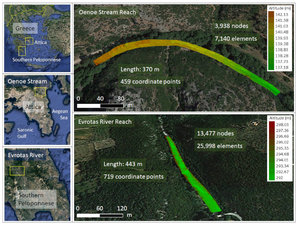
Figure 1.
Location of the two study areas. The Oenoe Stream reach (southern Peloponnese) was mapped with 370 coordinate points, and an unstructured computational mesh was developed consisting of 3938 nodes and 7140 triangular elements. The Evrotas River reach (Attica) was mapped with 719 coordinate points and the developed mesh consisted of 13477 nodes and 25998 elements.

Figure 2.
Assemblage-based macroinvertebrate habitat suitability for water temperature based on 380 microhabitats [21]. The blue line represents the cubic-splines-based, sine-shaped curve that best fitted the data (p < 0.001; R2 = 0.42).
Figure 2.
Assemblage-based macroinvertebrate habitat suitability for water temperature based on 380 microhabitats [21]. The blue line represents the cubic-splines-based, sine-shaped curve that best fitted the data (p < 0.001; R2 = 0.42).

Figure 3.
Macroinvertebrate habitat suitability in the Oenoe Stream (losing watershed) for 0%, 25% (Q = 0.45 m3/s), 50% (Q = 0.3 m3/s), 75% (Q = 0.15 m3/s), 90% (Q = 0.06 m3/s) discharge change from current average (Q = 0.61 m3/s) and near-dry flows (99%; Q = 0.006 m3/s) in the various water temperature change scenarios (1.6–1.8 °C, 2–2.5 °C, 3–5 °C, >5 °C). The dashed red line indicates the suitable habitat suitability limit (HSI > 0.6 corresponding to good and high classes). Environmental flows have been highlighted by a different pattern; discharges resulting to unsuitable habitats (HSI ≤ 0.6) have been colored orange.

Figure 4.
Macroinvertebrate habitat suitability in the Oenoe Stream for the six Intergovernmental Panel on Climate Change SRES scenarios [17], as adapted by [7] using three general circulation models (CNCM3, ECHAM, IPSL) (left pane) and (ii) the six extreme change scenarios developed in this study (right pane). The numbers below each map correspond to a change in discharge (%) | water temperature (°C).

Figure 5.
Macroinvertebrate habitat suitability in the Oenoe Stream (losing watershed) for 0%, 25% (Q = 0.45 m3/s), 50% (Q = 0.3 m3/s), 75% (Q = 0.15 m3/s), 90% (Q = 0.06 m3/s) discharge change from current average (Q = 0.61 m3/s) and near-dry flows (99%; Q = 0.006 m3/s) in the various water temperature change scenarios (1.6–1.8 °C, 2–2.5 °C, 3–5 °C, > 5 °C). The dashed red line indicates the suitable habitat suitability limit (HSI > 0.6 corresponding to good and high classes). Environmental flows have been highlighted by a different pattern; discharges resulting to unsuitable habitats (HSI ≤ 0.6) have been colored orange.

Figure 6.
Macroinvertebrate habitat suitability in the Evrotas River (winning watershed) for (i) the six Intergovernmental Panel on Climate Change SRES scenarios [17], as adapted by [7] using three general circulation models (CNCM3, ECHAM, IPSL) and (ii) the six extreme change scenarios developed in this study. The numbers below each map correspond to a change in discharge (%) | water temperature (°C).

Figure 7.
Winning (Evrotas River) and losing (Oenoe Stream) watershed recurring trends. A specific habitat suitability trend is repeated across discharge scenarios as water temperature increases, with overall declining suitability values but with the same suitability variation.
Figure 7.
Winning (Evrotas River) and losing (Oenoe Stream) watershed recurring trends. A specific habitat suitability trend is repeated across discharge scenarios as water temperature increases, with overall declining suitability values but with the same suitability variation.

Table 1.
The 12 climate change scenarios studied; six IPCC-based (SRES) scenarios [17] adapted by [7] (using three General Circulation Models, the CNCM3, ECHAM and IPSL) and six extreme-case scenarios.
| Climate Change Scenarios for 2071–2100 | Mean Discharge Change for 2071–2100 Compared to Current (%) | Mean Water Temperature Change for 2071–2100 Compared to Current (°C) | Evrotas-Specific Discharge (m3/s) | Evrotas-Specific Temperature (°C) | Oenoe-Specific Discharge (m3/s) | Oenoe-Specific Temperature (°C) |
|---|---|---|---|---|---|---|
| Standard (IPCC; [7,17]) | ||||||
| SRES B1/CNCM3 | 25–50 | 1.6–1.8 | 1.25 | 17.06 | 0.3 | 18.06 |
| SRES B1/ECHAM | 25–50 | 2–2.5 | 1.25 | 17.96 | 0.3 | 18.96 |
| SRES B1/IPSL | 0–25 | 2–2.5 | 1.875 | 17.96 | 0.45 | 18.96 |
| SRES A2/CNCM3 | >50 | 3–5 | 0.625 | 18.96 | 0.15 | 19.96 |
| SRES A2/ECHAM | >50 | 2–2.5 | 0.625 | 17.96 | 0.15 | 18.96 |
| SRES A2/IPSL | 25–50 | 3–5 | 1.25 | 18.96 | 0.3 | 19.96 |
| Extreme scenarios (study-specific) | ||||||
| EXT1 | 90 | 2–2.5 | 0.25 | 17.96 | 0.06 | 18.96 |
| EXT2 | 90 | 3–5 | 0.25 | 18.96 | 0.06 | 19.96 |
| EXT3 | 90 | >5 | 0.25 | 20.46 | 0.06 | 21.46 |
| EXT4 | 99 | 2–2.5 | 0.025 | 17.96 | 0.006 | 18.96 |
| EXT5 | 99 | 3–5 | 0.025 | 18.96 | 0.006 | 19.96 |
| EXT6 | 99 | >5 | 0.025 | 20.46 | 0.006 | 21.46 |
Publisher’s Note: MDPI stays neutral with regard to jurisdictional claims in published maps and institutional affiliations. |
© 2021 by the authors. Licensee MDPI, Basel, Switzerland. This article is an open access article distributed under the terms and conditions of the Creative Commons Attribution (CC BY) license (https://creativecommons.org/licenses/by/4.0/).
Share and Cite
MDPI and ACS Style
Theodoropoulos, C.; Karaouzas, I.; Stamou, A. Environmental Flows as a Proactive Tool to Mitigate the Impacts of Climate Warming on Freshwater Macroinvertebrates. Water 2021, 13, 2586. https://doi.org/10.3390/w13182586
AMA Style
Theodoropoulos C, Karaouzas I, Stamou A. Environmental Flows as a Proactive Tool to Mitigate the Impacts of Climate Warming on Freshwater Macroinvertebrates. Water. 2021; 13(18):2586. https://doi.org/10.3390/w13182586
Chicago/Turabian StyleTheodoropoulos, Christos, Ioannis Karaouzas, and Anastasios Stamou. 2021. "Environmental Flows as a Proactive Tool to Mitigate the Impacts of Climate Warming on Freshwater Macroinvertebrates" Water 13, no. 18: 2586. https://doi.org/10.3390/w13182586
Note that from the first issue of 2016, this journal uses article numbers instead of page numbers. See further details here.