
Aquifer Storage and Recovery in Layered Saline Aquifers: Importance of Layer-Arrangements


1
College of Water Conservancy and Hydropower Engineering, Hohai University, Nanjing 210098, China
2
State Key Laboratory of Hydrology-Water Resources and Hydraulic Engineering, Hohai University, Nanjing 210098, China
*
Author to whom correspondence should be addressed.
Water 2021, 13(18), 2595; https://doi.org/10.3390/w13182595
Submission received: 1 September 2021
/
Revised: 17 September 2021
/
Accepted: 18 September 2021
/
Published: 20 September 2021
(This article belongs to the Section Hydrogeology)
Abstract
:Aquifer storage and recovery (ASR) refers to injecting freshwater into an aquifer and later withdrawing it. In brackish-to-saline aquifers, density-driven convection and fresh-saline water mixing lead to a reduced recovery efficiency (RE, i.e., the volumetric ratio between recovered potable water and injected freshwater) of ASR. For a layered aquifer, previous studies assume a constant hydraulic conductivity ratio between neighboring layers. In order to reflect the realistic formation of layered aquifers, we systematically investigate 120 layered heterogeneous scenarios with different layer arrangements on multiple-cycle ASR using numerical simulations. Results show that the convection (as is reflected by the tilt of the fresh-saline interface) and mixing phenomena of the ASR system vary significantly among scenarios with different layer arrangements. In particular, the lower permeable layer underlying the higher permeable layer restricts the free convection and leads to the spreading of salinity at the bottom of the higher permeable layer and early salt breakthrough to the well. Correspondingly, the RE values are different among the heterogeneous scenarios, with a maximum absolute RE difference of 22% for the first cycle and 9% for the tenth cycle. Even though the difference in RE decreases with more ASR cycles, it is still non-negligible and needs to be considered after ten ASR cycles. The method to homogenize the layered heterogeneity by simply taking the arithmetic and geometric means of the hydraulic conductivities among different layers as the horizontal and vertical hydraulic conductivities is shown to overestimate the RE for multiple-cycle ASR. The outcomes of this research illustrate the importance of considering the geometric arrangement of layers in assessing the feasibility of multiple-cycle ASR operations in brackish-to-saline layered aquifers.
1. Introduction
Aquifer storage and recovery (ASR) refers to injecting freshwater into an aquifer for temporary water storage when freshwater is in surplus, and later withdrawal at shortfalls of freshwater supply using the same or, less commonly, a nearby well [1,2,3,4]. ASR schemes typically include three phases: (1) injection phase, when there is excess freshwater available to be injected into the aquifer; (2) storage phase, when neither injection nor pumping is performed; and (3) recovery phase, when the freshwater supply is at shortfall and the injected freshwater is withdrawn [5]. ASR provides a possibility to balance seasonal freshwater supply and demand without extra land acquisition or in-stream barriers, and it avoids the evaporation that occurs in surface water reservoirs [6]. Other advantages of ASR include large storage volumes, a reduced threat of contamination from natural and anthropogenic sources, less environmental impacts compared to the surface storage options, lower costs and technical resources requirements, and reduced seawater intrusion and reuse of desalinated seawater in coastal areas [7,8,9,10,11]. The performance of ASR can be impacted by clogging issues, geochemical processes, hydrogeological conditions, hydrodynamic dispersion, and wellfield design and operation parameters [12,13,14,15,16,17].
The performance of ASR is most commonly evaluated by the calculation of recovery efficiency (RE [%]), defined as [18]:
where Vinj [L3] is the volume of injected freshwater during a single ASR cycle, and Vrec [L3] is the recovered volume of potable water during the same ASR cycle. RE is calculated after each ASR cycle. Each ASR cycle includes the injection, storage, and recovery phases. RE values are reported to range from 0 to 100% [19,20,21,22]. Extreme values close to 0 indicate that ASR is not feasible under local aquifer conditions and ASR practices.
Since ASR is often implemented in brackish or saline aquifers located in coastal or semi-arid and arid areas [7,23,24,25], RE is reduced due to density-driven free convection and mixing of saline water with freshwater. Esmail and Kimbler [26] investigated the feasibility of ASR in confined homogeneous isotropic saline aquifers by performing an analytical analysis. They found that storing freshwater in saline aquifers is feasible, yet, RE is reduced due to density-driven convection which leads to a tilted fresh-saline interface and an early salt breakthrough at the bottom of the ASR well.
Ward et al. [27] conducted the mixed convection analysis of ASR. In their models, the pumping-induced forced convection and density-driven free convection simultaneously control the flow during injection and recovery, whereas flow during storage is only controlled by the free convection. The density effect was quantified by the dimensionless mixed convection ratio of buoyancy (arising from the density differences of injected freshwater and native saline water) to advective (driven by pumping) forces during the injection phase [27]:
where K [LT−1] is the hydraulic conductivity, B [L] is the confined aquifer thickness, Q [L3T−1] is the pumping rate, [-] is the density difference ratio, which equals to , ρs [ML−3] is the density of the native saline groundwater, ρf [ML−3] is the density of injected freshwater, θ [-] is the effective porosity, and ti [T] is the duration of the injection phase. A higher M value indicates a stronger intensity of density-driven convection and it leads to an earlier saline water breakthrough at the bottom of the ASR well during recovery phases, thereby reducing the RE [27].
Since natural aquifers are heterogeneous and a different K value results to a different density effect (refer to Equation (2)), Ward et al. [28] investigated a layered aquifer incorporating successive horizontal, isotropic layers with alternating low and high hydraulic conductivities. The isotropic hydraulic conductivity K in Equation (2) was replaced with the averaged vertical hydraulic conductivity Kzave (geometric mean of hydraulic conductivities of all stratum). In addition, a dimensionless Rayleigh number was introduced to characterize the relative contributions of density-driven convection versus dispersion (by neglecting diffusion) during the storage phase [28]:
where αL [L] is the longitudinal dispersivity. The performance of ASR was found to be sensitive to the layering patterns. Since density-driven convection can be suppressed by the low permeability layer underlying the high permeability layer, a higher RE value was obtained for the scenario with greater hydraulic conductivity contrast between the neighboring layers. Ward et al. [28] also suggested that layered heterogeneity can be simplified to homogeneous anisotropy by taking the geometric mean and arithmetic mean (respectively) of the hydraulic conductivities of all stratum as the vertical and horizontal hydraulic conductivities for the whole domain. Although this method led to an overestimation of RE in early cycles, they found that the long-term ASR RE (i.e., after ten ASR cycles) was not overestimated [28].
One limitation in Ward et al. [28] is the assumption of the specified constant ratio of hydraulic conductivities between every two neighboring layers. A realistic distribution of heterogeneous layers in natural aquifers is more complex. For example, the tertiary limestone injection zone at the Hialeah test site (Hialeah, Dade County, FL, USA) is composed of three layers of different thickness, and different horizontal and vertical hydraulic conductivities [29]. The ASR performance in such more realistic conditions remains unknown.
The present study aims to extend the knowledge of multiple-cycle ASR implemented in heterogeneous layered saline aquifers, particularly about the effect of multiple layer arrangements on flow and transport phenomena and RE. This is achieved through numerical simulations of hypothetical scenarios that are modified versions of those adopted in previous studies (e.g., [27,28]). The outcomes gained from this research are expected to improve the planning and feasibility assessment of ASR in heterogeneous layered brackish-to-saline aquifers.
2. Conceptual Model
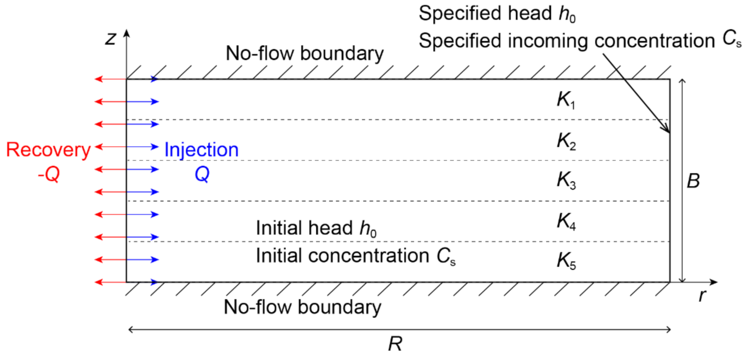
The current analysis considered axisymmetric groundwater flow and transport, which can be simulated in cross-section by multiplying K, θ and specific storage (Ss [L−1]) of each cell by 2πr (where r [L] is taken as the distance between the axis of symmetry and the center of the cell) to account for the increased flow area and cell volume with radial distance from the well [30]. The conceptual model adopted in this study, as shown in Figure 1, is based on the model in Ward et al. [28]. We divided the model domain into five horizontal layers with equal thickness. However, the hydraulic conductivities of all layers are different (K1 ≠ K2 ≠ K3 ≠ K4 ≠ K5). We investigated 120 scenarios including all possible arrangements of layers. Note that the contrast of conductivities between two neighboring layers is not limited to a constant in each scenario in this study, which is different from the identical conductivity contrast assumed in [28].
Both the top and bottom of the model are no-flow boundaries, representing impermeable confining beds. The left side of the model is set as the ASR well, which is simulated using a time-variant specified-flux boundary. The well boundary is composed of high vertical hydraulic conductivity cells (106 m/d) with θ set to unity. During the injection and recovery phases, the pumping rate is specified to 500 m3/d (Q, indicated with blue arrows in Figure 1) and −500 m3/d (−Q, indicated with red arrows in Figure 1), respectively. The fluxes that enter/leave the aquifer through the well zone are distributed uniformly across the entire well depth (i.e., the entire aquifer thickness). During the storage phase, the well boundary is converted to a no-flow boundary and the pumping rate is zero. Such settings of the well boundary are used following Maliva et al. [7] and Kang et al. [31]. The solute concentration of the water entering the model by injection (left boundary) is specified as zero (i.e., Ci = 0). The right side of the model domain is designated as a specified-head boundary with hydrostatic head distribution reflecting the density of the native saline water (i.e., h0 = 100 m). Groundwater entering the model through the right boundary has a concentration of Cs = 10 g/L, which is at the moderate range of that applied in previous ASR studies (2–28 g/L; e.g., [19,27,28]). At the start of the first ASR cycle, the aquifer is saturated with native saline water with a concentration of Cs. The initial head is h0, which is larger than the aquifer thickness (B = 50 m) to guarantee the confined aquifer condition.
3. Numerical Modelling
The present study applied the variable-density, finite-difference code SEAWAT-2000 [32], which solves coupled density-dependent flow and transport equations by combining MODFLOW-2000 [33] and MT3DMS [34]. It was successfully verified by comparing to several variable-density flow and transport benchmark problems [35], and was employed in numerical simulations of ASR (e.g., [7]).
3.1. Governing Equations
The governing equation for saturated density-dependent flow is expressed as [32]:
where ρ [ML−3] is the fluid density, h [L] is the water head, t [T] is time, z [L] is the vertical coordinate directed upward, ρss [ML−3] is the source/sink density, and qss [T−1] is the sink/source flow rate per unit volume of the aquifer.
The governing equation for non-reactive advective-dispersive transport is expressed as [34]:
where C [ML−3] is the solute concentration, D [L2T−1] is the hydrodynamic dispersion coefficient tensor, and v [LT−1] is the pore water velocity vector.
3.2. Model Discretization and Solver Setup
The model domain was uniformly discretized in the vertical direction with a cell thickness of 0.5 m. The 250-m radius of the model was subdivided into 410 columns with increasing cell widths, namely 0.2 m (r = 0 to 20 m), 0.5 m (r = 20 to 100 m), and 1 m (r = 100 to 250 m). The largest cell width meets the requirement that ∆r < 4αL (with αL equals 0.3 m), such that the numerical dispersion arising from truncation errors is avoided [34].
The duration of each ASR cycle was 365 days, comprising 100 days of injection, 165 days of storage, and 100 days of recovery. Similar to the approach of Bakker [20], the recovery pumping was terminated (i.e., −Q = 0) for the remainder of the ASR cycle once the salinity of recovered water exceeded a predefined value of 0.3 g/L. This value is regarded as the limit of potability (e.g., [7,27,28]). Therefore, RE is controlled by the pumping duration in the recovery phase. Ten consecutive cycles of ASR were simulated, which is a typical timeframe considering long-term ASR schemes (e.g., [28,36]).
The preconditioned conjugate gradient (PCG) solver was used with a head convergence criterion of 10−4 m, and the flow convergence criterion was set to 10−4 m3/d. For the transport equation, the generalized conjugate gradient (GCG) solver was used with the third-order total-variation-diminishing (TVD) scheme [37] to solve the advection term and for automatic timestep control (with courant number set to 0.9). TVD scheme is preferred here, because it is inherently mass conservative and does not introduce excessive numerical dispersion and artificial oscillation [34]. The concentration convergence criterion was set to 10−9 g/L.
3.3. Input Parameters and Scenarios
The adopted parameters of simulated cases were similar to those of [28], and they are listed in Table 1.
In total, 120 scenarios were simulated with different arrangements of the horizontal isotropic layers. We use EL, L, M, H, and EH to describe the degree of permeability (see Table 1), and each scenario can be indicated by an ordered combination of these texts. For instance, ‘EL-L-M-H-EH’ represents the scenario where the hydraulic conductivities monotonically increase from the top to bottom layers of the aquifer. The geometric mean and arithmetic mean of the isotropic hydraulic conductivities of layers (i.e., Krave and Kzave respectively) are identical among the 120 scenarios, which are calculated as:
These two average conductivity values were employed in the equivalent homogeneous anisotropic case.
4. Results and Discussion
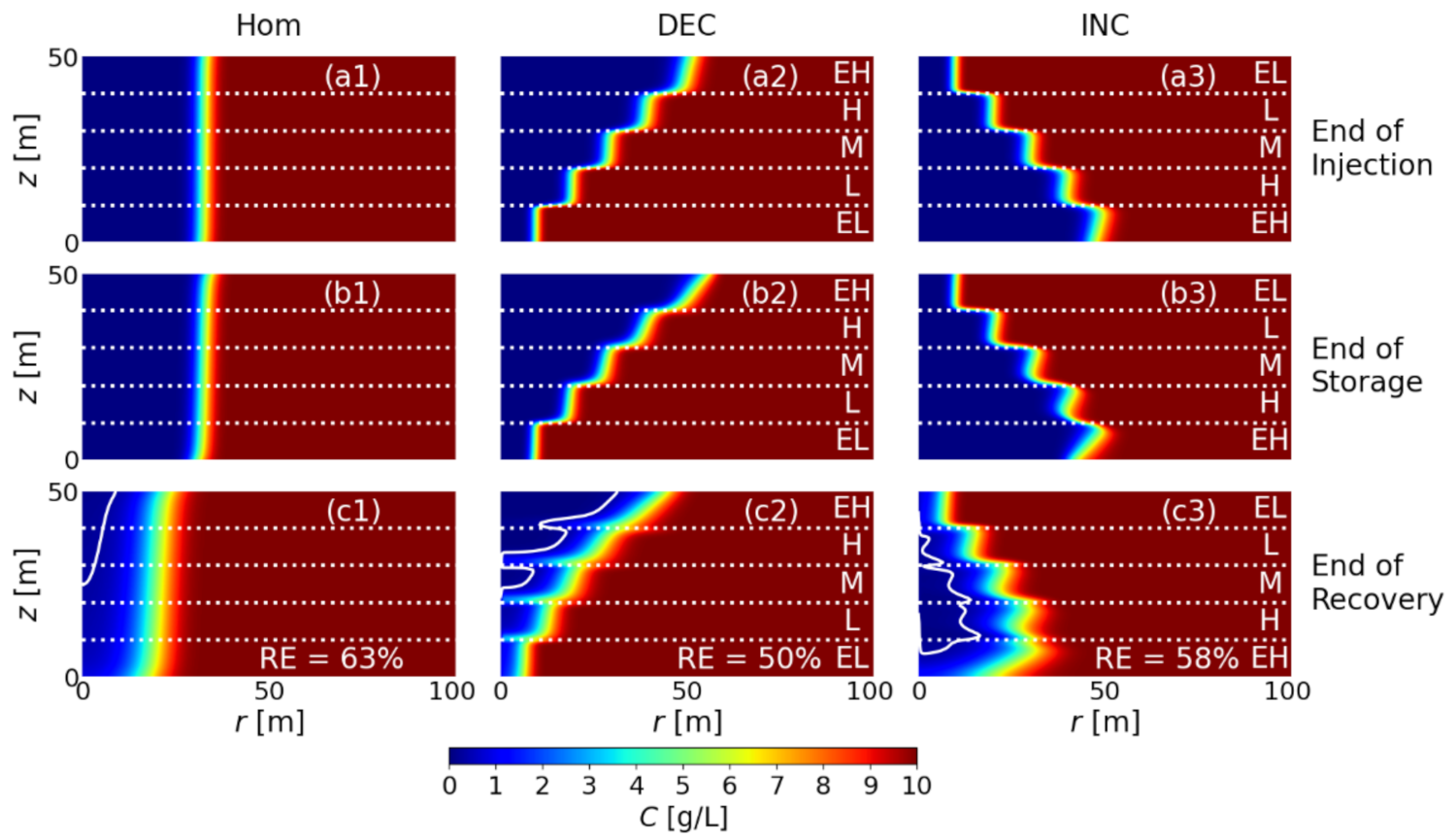
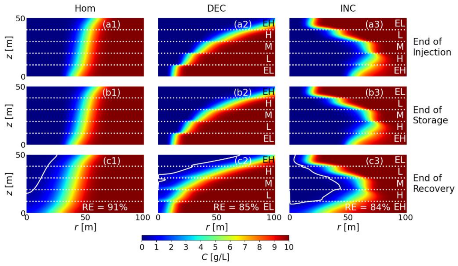
Figure 2 shows the salinity distributions for the equivalent homogeneous anisotropic case ‘Hom’, and heterogeneous cases ‘DEC’ (monotonically decreasing hydraulic conductivities with aquifer depth for the five layers, EH-H-M-L-EL) and ‘INC’ (monotonically increasing hydraulic conductivities with aquifer depth for the five layers, EL-L-M-H-EH) at the end of injection, storage, and recovery phases for the first ASR cycle. Contours of C = 0.3 g/L (white lines) are plotted in the recovery phase, with the RE values listed at the bottom of each scenario.
The aquifer in the ‘Hom’ case can be considered as five layers of identical hydraulic conductivity. In this case, the injected freshwater forms a vertical zone around the ASR well in the injection phase (see the dark blue zone in Figure 2(a1)). This indicates relative low density effect during injection, and it is consistent to the small value of mixed convection ratio (M = 8.772 × 10⁻³). The boundary of this zone is slightly tilted at the end of the storage phase due to the density effect and its resulting free convection (Figure 2(b1)). At this phase, the Rayleigh number equals to 1.462, representing the fact that density effect and dispersion have a similar magnitude during storage. The tilt of the interface is magnified in the recovery phase as a result of a combined effect from pumping, free convection and time (Figure 2(c1)). The mixing zone between the freshwater and saline water can be visualized by the gradual color changes shown in Figure 2. The mixing zone is narrow during the injection and storage phases, yet it becomes much wider in the recovery phase. The difference between the injection and recovery phases can be explained by the different combination of the directions between longitudinal dispersion and advection. Whereas the direction of longitudinal dispersion is invariably pointing from saline water to freshwater (right to left in Figure 2), injection leads to the advection from left to right and extraction from right to left. The opposite directions between longitudinal dispersion and advection in injection phase results to the suppression of mixing zone extension. In contrast, the identical direction between longitudinal dispersion and advection during recovery enhanced the mixing between the freshwater and saline water. As a result of the coupled effect from density difference and dispersion, the saline water intrudes into the lower half of the well (see contour line of C = 0.3 g/L in Figure 2(c1)). This leads to a limited RE of 63%, significantly lower than 100%.
For heterogeneous cases, the injected freshwater preferentially enters to the high permeable layers, forming ‘ladder’ like injectant plumes. The radius of the injectant plume monotonically decreases with aquifer depth in the ‘DEC’ case (Figure 2(a2)) and it monotonically increases with aquifer depth in the ‘INC’ case (Figure 2(a3)). The tilting of the fresh-saline interface is more remarkable in the layer with higher hydraulic conductivity (Figure 2(b2,b3)). For instance, the fresh-saline interface is most tilted in the ‘EH’ layer, while it looks vertical in the ‘EL’ layer. Such a phenomenon indicates a stronger density effect for the higher permeable condition. Furthermore, the widths of the mixing zone are larger in the layers with higher hydraulic conductivity. This is caused by the higher flow velocity and dispersion in the higher permeable layer. Again, the mixing zone width is the widest in the ‘EH’ layer and it is the narrowest in the ‘EL’ layer.
The mixing zones of the two heterogeneous cases are also extended during the recovery phase. Yet, there are differences in the salt breakthrough behavior between the two cases. For the ‘DEC’ case, the contour of C = 0.3 g/L intrudes the well zone through the bottom of the ‘H’ layer, as well as the lower half of the aquifer (Figure 2(c2)). In contrast, for the ‘INC’ case, the contour intrudes the well zone through the ‘EH’ and ‘EL’ layers (i.e., the bottom and top of the aquifer; Figure 2(c3)). This leads to different RE values for the two heterogeneous cases (i.e., 50% and 58%, respectively). As is expected, RE is lower for the heterogenous case than that of the equivalent homogenous case.
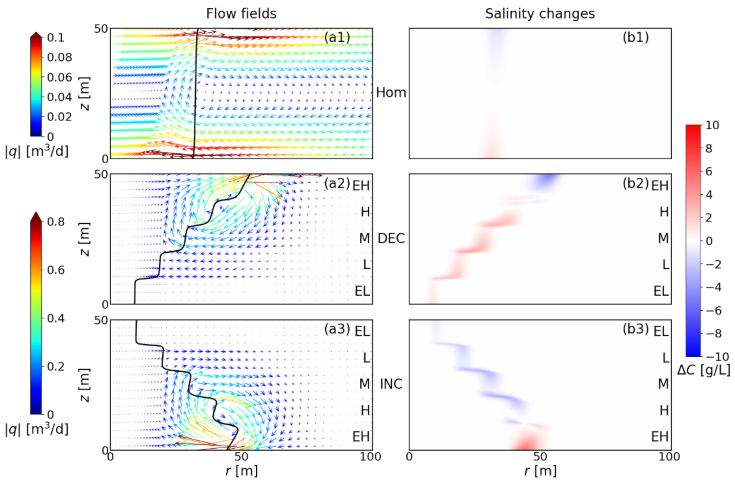
In order to explain the breakthrough behavior observed in Figure 2, we investigated flow velocity distributions and salinity changes during the storage and recovery phases for the two heterogeneous cases and the equivalent homogeneous case. Figure 3 shows the flow field at the intermediate storage phase (i.e., after 82 days of storage; left) and the salinity changes during the storage phase (right) for the ‘Hom’, ‘DEC’, and ‘INC’ cases in the first ASR cycle. The salinity changes are calculated as the concentration difference (ΔC) between the end and start of the storage phase. In the flow fields subplots, the contour of C = 5 g/L is plotted as black lines to roughly indicate the fresh-saline interface.
As shown by the flow vectors in Figure 3(a1), free convection is observed for the ‘Hom’ case. Even though the flow rate is very small (up to 0.1 m3/d), flow from right to left in the lower aquifer leads to the salinization of the injected freshwater. Subsequently, it leads to the flow from left to right in the upper aquifer, resulting to a decrease in salinity. Such a flow condition is also reflected by the slight tilting of the fresh-saline interface shown in Figure 2(b1).
For heterogeneous cases, the flow field is more complex. In particular, a rotating flow regime is observed at relatively high permeable layers in each heterogeneous case. In both heterogeneous cases, the rotation happens at the fresh-saline interface and the rotating direction is clockwise. The highest flow velocity happens at the fresh-saline interface of the most permeable layer. The variation of flow velocities in the heterogenous cases is up to 0.8 m3/d, much larger than that in the ‘Hom’ case. Such complex flow conditions formed in the heterogeneous cases result to remarkable salinity changes during the storage phase. In the ‘DEC’ case, salinity increases in the bottom four layers and decreases in the top one layer (Figure 3(b2)). Since the hydraulic conductivity is higher in the upper layer compared to the neighboring lower layer, the density effect is restricted by the lower layer and leads to a spreading of salinity at the bottom of each layer. In contrast, for the ‘INC’ case, salinity decreases in the top four layers and increases in the bottom one layer (Figure 3(c2)). Nevertheless, due to density effect, salinity always increases in the lower part of the aquifer and decreases in the upper part of the aquifer for all the homogeneous and heterogeneous cases.
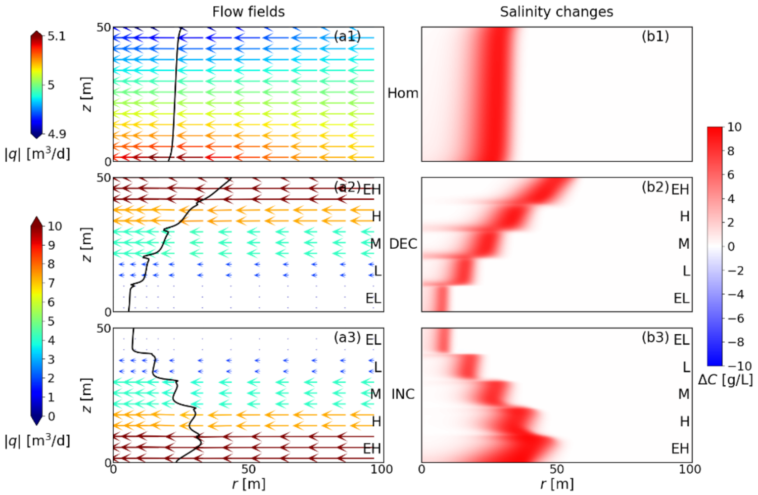
Figure 4 shows the flow fields at the intermediate recovery phase (i.e., after 50 days of recovery) and the salinity changes during the recovery phase for the ‘Hom’, ‘DEC’, and ‘INC’ cases in the first ASR cycle. Flow vectors appear horizontal and convergent, indicating the domination of pumping-induced forced convection. For the ‘Hom’ case, the flow velocity decreases as z increases (Figure 4(a1)). This is because the free convection caused by the density effect reinforces the convergent flow in the lower aquifer and retarded that in the upper aquifer. Such a mixed convection leads to a slightly fast transport of salinity to the well in the lower aquifer (Figure 4(b1)), leading to a smaller than 100% RE value.
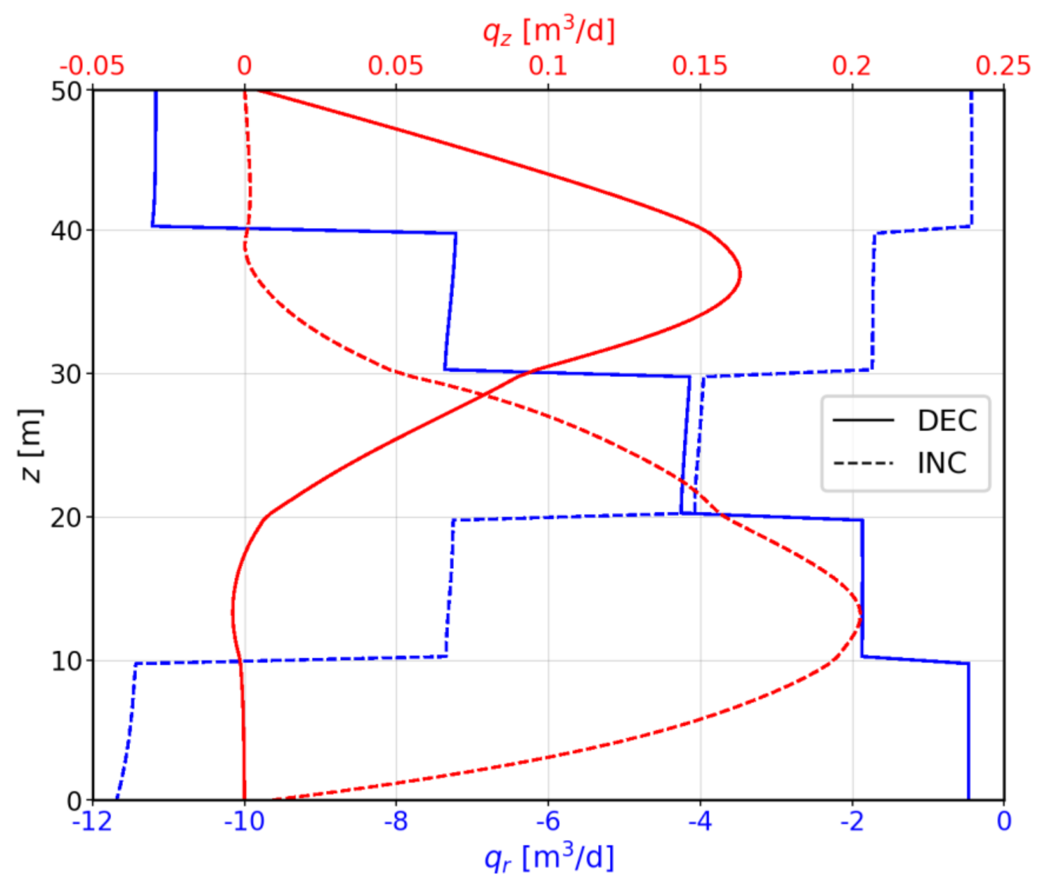
For the heterogeneous cases, flow is significantly faster in the higher permeable layer (Figure 4(a2,a3)). However, the gradual change of flow velocities in every single layer is not observable. In order to illustrate the existence of free convection, we depicted the horizontal flow qr and vertical flow qz at the vertical cross-section of r = 20 m in Figure 5. As shown by the red lines, qz varies significantly along the vertical direction and shows a relatively high value at the high permeable zones. Such a phenomenon is consistent with that shown in the storage phase (see Figure 3(a2,a3)), indicating complex flow conditions in the recovery phase for the two heterogeneous cases. Additionally, the qr values in the ‘EH’ layers are different between the two heterogeneous cases. The faster qr in the ‘INC’ case is the result of summation between forced and free convection, whereas the slower qr in the ‘DEC’ case is caused by the subtraction of flow velocity due to the density effect from forced convection.
The spreading of salinity at the bottom of each layer in the ‘DEC’ case (see Figure 4(b2)) is again due to the restriction of density effect by the lower permeable layer underlying the higher permeable layer. And the spreading is enhanced by the pumping-induced advection. Such spreading of salinity causes a breakthrough and salt intrusion in the interfaces between the layers. For the ‘INC’ case, the spreading of the salt plume is not observed at layer interfaces. The intrusion of salt to the well zone in the bottom layer is caused by the faster forced convection and free convection, and the intrusion in the top layer is due to its small freshwater volume.
The salinity distributions for the equivalent homogeneous case (‘Hom’) and the two heterogeneous cases (‘DEC’ and ‘INC’) at the end of each phase for the tenth ASR cycle are demonstrated in Figure 6, with RE values listed and the contour of C = 0.3 g/L plotted in the recovery phase. As is indicated by the larger area of dark-blue zones (compared to that in the first cycle; see Figure 2), the aquifer near the well become fresher after ten cycles. As a result, the RE values increase. The RE values of the two heterogeneous cases (i.e., 85% and 84%) are still lower than that of the ‘Hom’ case (i.e., 91%). This implies that the effects of the layered heterogeneity cannot be eliminated with ten ASR cycles. For instance, the intrusion of salt at the layer interface keeps arising and it contributes to the reduction of RE for the ‘DEC’ case in the tenth cycle (Figure 6(c2)).
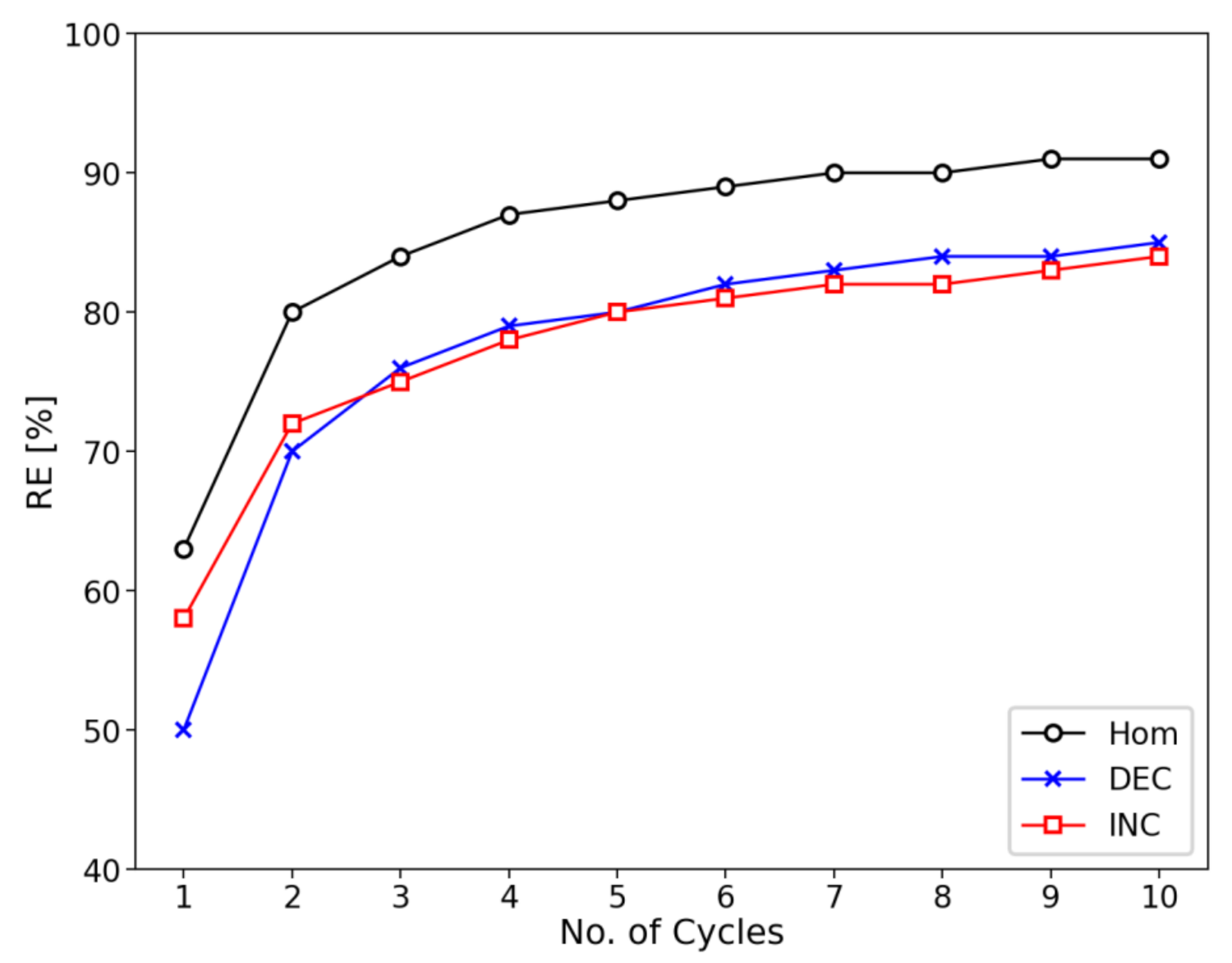
Figure 7 shows the RE values calculated at each cycle for the equivalent homogeneous case, and the heterogeneous cases ‘DEC’ and ‘INC’. RE increases with the number of cycles, as the aquifer continuously becomes fresher due to the cyclic injectant flushing. However, RE values are consistently lower for the heterogeneous cases than the homogeneous case regardless of the number of cycles. This indicates the impacts of layered heterogeneity on RE sustain even after ten ASR cycles.
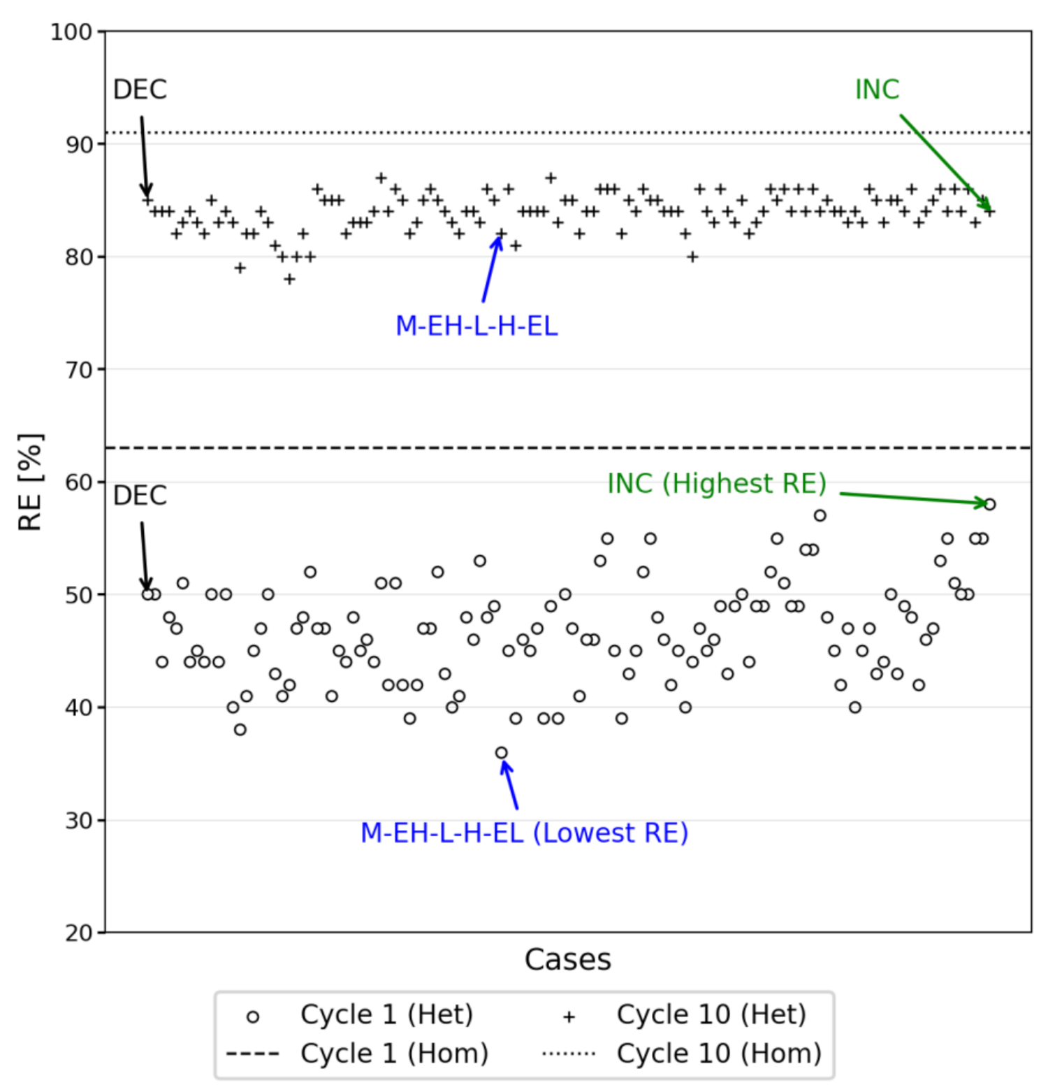
Figure 8 shows the RE values calculated at the first and tenth cycles for the equivalent homogeneous case (‘Hom’, lines) and the heterogeneous cases of all possible arrangements of the five isotropic layers (‘Het’, scattered points). The RE values of heterogeneous cases are always lower than those of the equivalent homogeneous case, both in the first and tenth cycles. This indicates that homogenizing the layered heterogeneity by simply replacing the averaged horizontal and vertical hydraulic conductivities (Krave and Kzave) overestimates the ASR RE under density-dependent conditions. Such an overestimation is reduced but still non-negligible after ten ASR cycles. Consistently, the absolute difference of RE values among different scenarios is up to 22% in the first cycle (shown as circles), but it reduces to a maximum absolute difference of 9% after ten ASR cycles (shown as crosses).
As shown in Figure 8, the highest RE obtained for the ‘INC’ case in the first cycle does not remain highest in the tenth cycle. Correspondingly, the lowest RE reached for the ‘M-EH-L-H-EL’ case ranges to a moderate order in the tenth cycle.
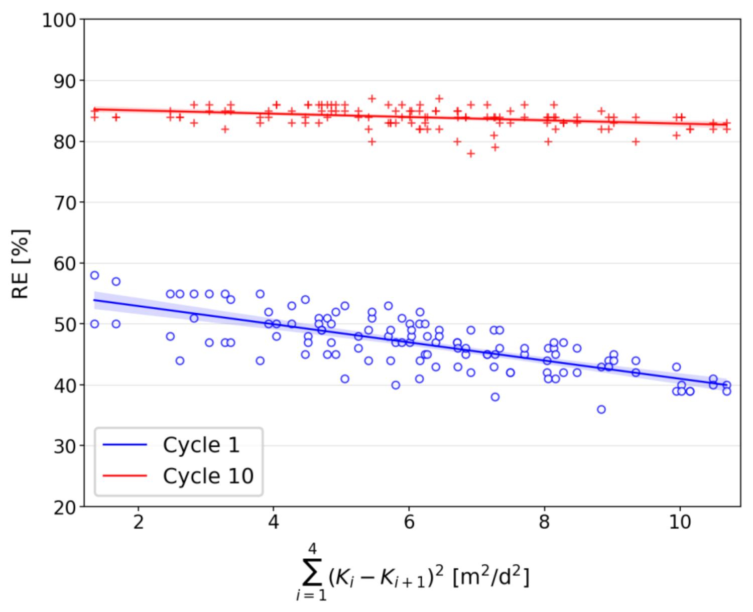
Recall that the density effect and free convection can be restricted in the higher permeable layer overlying the lower permeable layer and leads to the salinity spreading at the bottom of the higher permeable layer and thus salt intrusion to the well, we conjecture that there might be a relationship between RE and differences of hydraulic conductivities between neighboring layers. To verify this conjecture, the RE values are plotted versus the sum of squared hydraulic conductivity difference between neighboring layers (i.e., ) in Figure 9 as scattered points for the first (blue circles) and tenth (red crosses) ASR cycles. The straight lines that pass through the scattered points are obtained by the first-order linear regression with a confidence degree of 95%. In consistence with our conjecture, the RE values show a qualitatively decreasing trend with increasing values.
5. Conclusions
This study investigates the effects of layer-arrangements on multiple-cycle ASR in saline aquifers by numerical simulations coupling the density-dependent flow and advective-dispersive transport. The results show that the performance of ASR (i.e., RE) is significantly influenced by the heterogeneity and its geometric arrangements of isotropic layers with different hydraulic conductivities.
Free convection caused by the density effect results in a salinity increase in the lower part and a salinity decrease in the upper part of the homogeneous (in hydraulic conductivity) porous media zone, leading to a tilt of the fresh-saline interface. In addition, the longitudinal dispersion contributes to the mixing of freshwater and saline water and creates significant mixing zones, particularly during the recovery phase. The combination of the density effect and mixing leads to a smaller than 100% RE value. Both the density effect and mixing are more significant in high permeable layers, thus creating complex flow fields in layered heterogeneous aquifers. In particular, a rotating flow is observed in the selected heterogeneous cases of ‘DEC’ and ‘INC’. RE is limited in heterogenous conditions by the early salt breakthrough at the layer interface. This is achieved by the restriction of free convection by the lower permeable layer underlying the higher permeable layer and the salt spreading at the bottom of the higher permeable layer.
Although the values of M and Ra remain the same for all 120 heterogeneous scenarios, RE is significantly different from each other. The difference is reduced after ten ASR cycles, but it is non-negligible. Furthermore, homogenizing the layered heterogeneity by replacing the horizontal and vertical hydraulic conductivities, respectively, with the arithmetic mean and geometric mean of hydraulic conductivities of the heterogeneous layers overestimates the RE of multiple-cycle ASR in saline aquifers.
For those interested in using numerical modelling to assess the feasibility of multiple-cycle ASR projects implemented in layered saline aquifers, neglecting the formation of the layered heterogeneity (i.e., arrangement of layers) is problematic. However, existing site selection indexes for ASR schemes (used to determine the feasibility of ASR operations) implemented in saline aquifers lack the consideration of layer-arrangements (see the review paper [22]). Therefore, future work is worthwhile to include the information of layer-arrangements in coming up with a site selection index of multiple-cycle ASR operations implemented in brackish-to-saline aquifers.
Author Contributions
Conceptualization, H.L., Y.Y. and C.L.; methodology, H.L.; software, H.L.; validation, H.L., Y.Y. and C.L.; formal analysis, H.L.; investigation, H.L.; writing—original draft preparation, H.L.; writing—review and editing, Y.Y.; visualization, H.L.; supervision, C.L.; project administration, C.L.; funding acquisition, Y.Y. and C.L. All authors have read and agreed to the published version of the manuscript.
Funding
This research was funded by the National Natural Science Foundation of China (51879088) and the Fundamental Research Funds for the Central Universities (B200202158).
Acknowledgments
This study was supported by High Performance Computing Platform, Hohai University.
Conflicts of Interest
The authors declare no conflict of interest.
References
- Pyne, R.D.G.; Horvath, L.E.; Pearce, M.S. Aquifer Storage and Recovery (ASR) Issues and Concepts. Position Paper Prepared for the St. Johns River Water Management District; ASR Systems LLC.: Gainesville, FL, USA, 2004; p. 37. [Google Scholar]
- Dillon, P. Future management of aquifer recharge. Hydrogeol. J. 2005, 13, 313–316. [Google Scholar] [CrossRef]
- Ringleb, J.; Sallwey, J.; Stefan, C. Assessment of Managed Aquifer Recharge through Modeling—A Review. Water 2016, 8, 579. [Google Scholar] [CrossRef] [Green Version]
- Maliva, R.G. ASR and Aquifer Recharge Using Wells. In Anthropogenic Aquifer Recharge; Springer: Berlin, Germany, 2020; pp. 381–436. [Google Scholar] [CrossRef]
- Maliva, R.G.; Guo, W.; Missimer, T.M. Aquifer storage and recovery: Recent hydrogeological advances and system performance. Water Environ. Res. 2006, 78, 2428–2435. [Google Scholar] [CrossRef]
- Almulla, A.; Hamad, A.; Gadalla, M. Aquifer storage and recovery (ASR): A strategic cost-effective facility to balance water production and demand for Sharjah. Desalination 2005, 174, 193–204. [Google Scholar] [CrossRef]
- Maliva, R.G.; Manahan, W.H.; Missimer, T.M. Aquifer Storage and Recovery Using Saline Aquifers: Hydrogeological Controls and Opportunities. Groundwater 2019, 58, 9–18. [Google Scholar] [CrossRef]
- National Research Council. Aquifer Storage and Recovery in the Comprehensive Everglades Restoration Plan: A Critique of Pilot Pro-jects and Related Plans for ASR in the Lake Okeechobee and Western Hillsboro Area; National Academy Press: Washington, DC, USA, 2001; p. 74. [Google Scholar] [CrossRef]
- National Research Council. Regional Issues in Aquifer Storage and Recovery for Everglades Restoration: A Review of the ASR Regional Study Project Management Plan of the Comprehensive Everglades Restoration Plan; National Academy Press: Washington, DC, USA, 2002; p. 75. [Google Scholar] [CrossRef]
- Shammas, M.I. The effectiveness of artificial recharge in combating seawater intrusion in Salalah coastal aquifer, Oman. Environ. Earth Sci. 2007, 55, 191–204. [Google Scholar] [CrossRef]
- Ganot, Y.; Holtzman, R.; Weisbrod, N.; Nitzan, I.; Katz, Y.; Kurtzman, D. Monitoring and modeling infiltration–recharge dynamics of managed aquifer recharge with desalinated seawater. Hydrol. Earth Syst. Sci. 2017, 21, 4479–4493. [Google Scholar] [CrossRef] [Green Version]
- Jeong, H.Y.; Jun, S.-C.; Cheon, J.-Y.; Park, M. A review on clogging mechanisms and managements in aquifer storage and recovery (ASR) applications. Geosci. J. 2018, 22, 667–679. [Google Scholar] [CrossRef]
- Greskowiak, J.; Prommer, H.; Vanderzalm, J.; Pavelic, P.; Dillon, P. Modeling of carbon cycling and biogeochemical changes during injection and recovery of reclaimed water at Bolivar, South Australia. Water Resour. Res. 2005, 41. [Google Scholar] [CrossRef] [Green Version]
- Bekele, E.; Page, D.; Vanderzalm, J.; Kaksonen, A.; Gonzalez, D. Water Recycling via Aquifers for Sustainable Urban Water Quality Management: Current Status, Challenges and Opportunities. Water 2018, 10, 457. [Google Scholar] [CrossRef] [Green Version]
- Lowry, C.S.; Anderson, M.P. An Assessment of Aquifer Storage Recovery Using Ground Water Flow Models. Ground Water 2006, 44, 661–667. [Google Scholar] [CrossRef] [PubMed]
- Zuurbier, K.G.; Zaadnoordijk, W.J.; Stuyfzand, P.J. How multiple partially penetrating wells improve the freshwater recovery of coastal aquifer storage and recovery (ASR) systems: A field and modeling study. J. Hydrol. 2014, 509, 430–441. [Google Scholar] [CrossRef]
- Zuurbier, K.G. Increasing Freshwater Recovery upon Aquifer Storage. A Field and Modelling Study of Dedicated Aquifer Storage and Recovery Con-figurations in Brackish Saline aquifers. Ph.D. Thesis, Delft University of Technology, Delft, The Netherland, 2016; p. 219. [Google Scholar] [CrossRef]
- Kimbler, O.K.; Kazmann, R.G.; Whitehead, W.R. Cyclic Storage of Fresh Water in Saline Aquifers. La. Water Resour. Res. Inst. Bull. 1975, 10, 78. [Google Scholar]
- Ward, J.D.; Simmons, C.T.; Dillon, P.J.; Pavelic, P. Integrated assessment of lateral flow, density effects and dispersion in aquifer storage and recovery. J. Hydrol. 2009, 370, 83–99. [Google Scholar] [CrossRef]
- Bakker, M. Radial Dupuit interface flow to assess the aquifer storage and recovery potential of saltwater aquifers. Hydrogeol. J. 2009, 18, 107–115. [Google Scholar] [CrossRef]
- Lu, C.; Du, P.; Chen, Y.; Luo, J. Recovery efficiency of aquifer storage and recovery (ASR) with mass transfer limitation. Water Resour. Res. 2011, 47. [Google Scholar] [CrossRef]
- Brown, C.J.; Ward, J.; Mirecki, J. A Revised Brackish Water Aquifer Storage and Recovery (ASR) Site Selection Index for Water Resources Management. Water Resour. Manag. 2016, 30, 2465–2481. [Google Scholar] [CrossRef]
- Saharawat, Y.S.; Chaudhary, N.; Malik, R.S.; Jat, M.L.; Singh, K.; Streck, T. Artificial Ground Water Recharge and Recovery of a Highly Saline Aquifer. Curr. Sci. 2011, 100, 1211–1216. [Google Scholar]
- Laattoe, T.; Werner, A.; Woods, J.; Cartwright, I. Terrestrial freshwater lenses: Unexplored subterranean oases. J. Hydrol. 2017, 553, 501–507. [Google Scholar] [CrossRef] [Green Version]
- Sendrós, A.; Urruela, A.; Himi, M.; Alonso, C.; Lovera, R.; Tapias, J.; Rivero, L.; Garcia-Artigas, R.; Casas, A. Characterization of a Shallow Coastal Aquifer in the Framework of a Subsurface Storage and Soil Aquifer Treatment Project Using Electrical Resistivity Tomography (Port de la Selva, Spain). Appl. Sci. 2021, 11, 2448. [Google Scholar] [CrossRef]
- Esmail, O.J.; Kimbler, O.K. Investigation of the technical feasibility of storing fresh water in saline aquifers. Water Resour. Res. 1967, 3, 683–695. [Google Scholar] [CrossRef]
- Ward, J.D.; Simmons, C.T.; Dillon, P.J. A theoretical analysis of mixed convection in aquifer storage and recovery: How important are density effects? J. Hydrol. 2007, 343, 169–186. [Google Scholar] [CrossRef]
- Ward, J.D.; Simmons, C.T.; Dillon, P.J. Variable-density modelling of multiple-cycle aquifer storage and recovery (ASR): Importance of anisotropy and layered heterogeneity in brackish aquifers. J. Hydrol. 2008, 356, 93–105. [Google Scholar] [CrossRef]
- Merritt, M.L. Recovering Fresh Water Stored in Saline Limestone Aquifers. Ground Water 1986, 24, 516–529. [Google Scholar] [CrossRef]
- Langevin, C.D. Modeling Axisymmetric Flow and Transport. Ground Water 2008, 46, 579–590. [Google Scholar] [CrossRef] [PubMed]
- Kang, P.; Lee, J.; Fu, X.; Lee, S.; Kitanidis, P.K.; Juanes, R. Improved characterization of heterogeneous permeability in saline aquifers from transient pressure data during freshwater injection. Water Resour. Res. 2017, 53, 4444–4458. [Google Scholar] [CrossRef] [Green Version]
- Langevin, C.D.; Shoemaker, W.B.; Guo, W. MODFLOW-2000, the U.S. Geological Survey Modular Ground-water Flow Model-Documentation of the SEAWAT-2000 Version with the Variable Density Flow Process (VDF) and the Integrated MT3DMS Transport Process (IMT). U.S. Geol. Surv. Open File Rep. 2003, 426, 43. [Google Scholar] [CrossRef]
- Harbaugh, A.W.; Banta, E.R.; Hill, M.C.; McDonald, M.G. MODFLOW-2000, The U.S. Geological Survey Modular Ground-Water Model—User Guide to Modularization Concepts and the Ground-Water Flow Process. U.S. Geol. Surv. Open File Rep. 2000, 92, 121. [Google Scholar] [CrossRef] [Green Version]
- Zheng, C.; Wang, P.P. MT3DMS: A Modular Three-dimensional Multispecies Model for Simulation of Advection, Dispersion and Chemical Reactions of Contaminants in Groundwater Systems: Documentation and User’s Guide. U.S. Army Corps Eng. Contract Rep 1999, SERDP-99-1, 202. [Google Scholar]
- Guo, W.; Langevin, C. User’s guide to SEAWAT; a computer program for simulation of three-dimensional variable-density ground-water flow. U.S. Geol. Surv. Open File Rep. 2001, 434, 77. [Google Scholar] [CrossRef]
- Culkin, S.L.; Singha, K.; Day-Lewis, F.D. Implications of Rate-Limited Mass Transfer for Aquifer Storage and Recovery. Ground Water 2008, 46, 591–605. [Google Scholar] [CrossRef] [PubMed]
- Harten, A. High resolution schemes for hyperbolic conservation laws. J. Comput. Phys. 1983, 49, 357–393. [Google Scholar] [CrossRef] [Green Version]
Figure 1.
Conceptual model of 2D axisymmetric flow and transport associated with ASR implemented in a confined five-layer aquifer.
Figure 1.
Conceptual model of 2D axisymmetric flow and transport associated with ASR implemented in a confined five-layer aquifer.

Figure 2.
Salinity distributions at the end of injection (a1–a3), storage (b1–b3), and recovery (c1–c3) phases for the first ASR cycle. Results shown are for the equivalent homogeneous anisotropic case (‘Hom’), the heterogeneous cases where isotropic hydraulic conductivity decreases from the aquifer top to the bottom (‘DEC’), and that increases from the aquifer top to the bottom (‘INC’). Salinity contours of C = 0.3 g/L are plotted as white lines on salinity plots at the end of recovery, with RE values listed.

Figure 3.
Flow field distributions at the intermediate storage phase (i.e., after 82 days of storage; a1–a3) and the salinity changes during storage (i.e., concentration difference between the end and start of the storage phase; b1–b3) for the first ASR cycle. Results shown are for the equivalent homogeneous case ‘Hom’ (top), and the heterogeneous cases ‘DEC’ (middle) and ‘INC’ (bottom). The black lines represent the contour of C = 5 g/L, indicating the approximate location of the fresh-saline interface.

Figure 4.
Flow vectors at the intermediate recovery phase (i.e., after 50 days of storage; a1–a3) and the salinity changes during storage (i.e., the difference between the concentration distribution at the end of the recovery phase and that at the start; b1–b3) for the first ASR cycle. Results shown are for the homogeneous anisotropic case ‘Hom’ (top), and the heterogeneous cases ‘DEC’ (middle) and ‘INC’ (bottom). The black lines represent the contour of C = 5 g/L, indicating the approximate location of the fresh-saline interface.

Figure 5.
Flow in the horizontal direction qr (blue) and vertical direction qz (red), for the heterogeneous cases ‘DEC’ (solid lines) and ‘INC’ (dashed lines). Results are assessed at r = 20 m that is approximately the average location of the fresh-saline interface.
Figure 5.
Flow in the horizontal direction qr (blue) and vertical direction qz (red), for the heterogeneous cases ‘DEC’ (solid lines) and ‘INC’ (dashed lines). Results are assessed at r = 20 m that is approximately the average location of the fresh-saline interface.

Figure 6.
Salinity distributions at the end of injection (a1–a3), storage (b1–b3), and recovery (c1–c3) phases for the tenth ASR cycle. Results shown are for the homogeneous anisotropic case (‘Hom’), the heterogeneous cases where isotropic hydraulic conductivities decrease from the aquifer top to the bottom (‘DEC’), and that increase from the aquifer top to the bottom (‘INC’). Salinity contours of C = 0.3 g/L are plotted as white lines on salinity plots at the end of recovery, with RE values listed.

Figure 7.
RE values calculated for ten ASR cycles for the homogenous (‘Hom’) and two heterogenous cases (‘DEC’ and ‘INC’).
Figure 7.
RE values calculated for ten ASR cycles for the homogenous (‘Hom’) and two heterogenous cases (‘DEC’ and ‘INC’).

Figure 8.
RE values assessed at the first and tenth cycles, for heterogeneous cases of all possible arrangements of the five isotropic layers (‘Het’, scattered points) and the homogeneous anisotropic case (‘Hom’, lines).
Figure 8.
RE values assessed at the first and tenth cycles, for heterogeneous cases of all possible arrangements of the five isotropic layers (‘Het’, scattered points) and the homogeneous anisotropic case (‘Hom’, lines).

Figure 9.
Distributions of the RE values versus the sum of squared hydraulic conductivity difference between neighboring layers for the first (blue circles) and tenth (red crosses) ASR cycles. The straight lines are obtained by the first-order linear regression with 95% confidence.
Figure 9.
Distributions of the RE values versus the sum of squared hydraulic conductivity difference between neighboring layers for the first (blue circles) and tenth (red crosses) ASR cycles. The straight lines are obtained by the first-order linear regression with 95% confidence.


Table 1.
Model input parameters.
| Parameter | Symbol | Value | Unit |
|---|---|---|---|
| Model radius | R | 250 | m |
| Model thickness | B | 50 | m |
| Cell width | ∆r | 0.2 to 1 | m |
| Cell thickness | ∆z | 0.5 | m |
| Uniform thickness of each layer | b | 10 | m |
| Isotropic hydraulic conductivities (for each layer) | K1 to K5 | 0.09 (EL), 0.36 (L), 0.82 (M), 1.46 (H), 2.27 (EH) | m/d |
| Horizontal hydraulic conductivity (average) * | Krave | 1 | m/d |
| Vertical hydraulic conductivity (average) * | Kzave | 0.06 | m/d |
| Longitudinal dispersivity | αL | 0.3 | m |
| Transverse dispersivity | αT | 0.03 | m |
| Molecular diffusion coefficient | Dd | 10−9 | m2/s |
| Specific storage | Ss | 10−4 | 1/m |
| Initial head | h0 | 100 | m |
| Injected water concentration | Ci | 0 | g/L |
| Native saline water concentration | Cs | 10 | g/L |
| Density difference ratio | 7.143 × 10⁻³ | - | |
| Effective porosity | θ | 0.3 | - |
| Injection/Recovery pumping rates | Q | 500 | m3/d |
| Injection duration | ti | 100 | d |
| Storage duration | ts | 165 | d |
| Recovery duration | tr | 100 | d |
| Mixed convection ratio | M | 8.772 × 10⁻³ | - |
| Rayleigh number | Ra | 1.462 | - |
* Applied to the equivalent homogeneous anisotropic case.
Publisher’s Note: MDPI stays neutral with regard to jurisdictional claims in published maps and institutional affiliations. |
© 2021 by the authors. Licensee MDPI, Basel, Switzerland. This article is an open access article distributed under the terms and conditions of the Creative Commons Attribution (CC BY) license (https://creativecommons.org/licenses/by/4.0/).
Share and Cite
MDPI and ACS Style
Li, H.; Ye, Y.; Lu, C. Aquifer Storage and Recovery in Layered Saline Aquifers: Importance of Layer-Arrangements. Water 2021, 13, 2595. https://doi.org/10.3390/w13182595
AMA Style
Li H, Ye Y, Lu C. Aquifer Storage and Recovery in Layered Saline Aquifers: Importance of Layer-Arrangements. Water. 2021; 13(18):2595. https://doi.org/10.3390/w13182595
Chicago/Turabian StyleLi, Hongkai, Yu Ye, and Chunhui Lu. 2021. "Aquifer Storage and Recovery in Layered Saline Aquifers: Importance of Layer-Arrangements" Water 13, no. 18: 2595. https://doi.org/10.3390/w13182595
Note that from the first issue of 2016, this journal uses article numbers instead of page numbers. See further details here.