Comprehensive Assessment Indicator of Ecosystem Resilience in Central Asia

Abstract

The ecosystems in the arid inland areas of Central Asia are fragile and severely degraded. Understanding and assessing ecosystem resilience is a challenge facing ecosystems. Based on the net primary productivity (NPP) data estimated by the CASA model, this study conducted a quantitative analysis of the ecosystem’s resilience and comprehensively reflected its resilience from multiple dimensions. Furthermore, a comprehensive resilience index was constructed. The result showed that plain oasis’s ecosystem resilience is the highest, followed by deserts and mountainous areas. From the perspective of vegetation types, the highest resilience is artificial vegetation and the lowest is forest. In warm deserts, the resilience is higher in shrubs and meadows and lower in grassland vegetation. High coverage and biomass are not the same as the strong adaptability of the ecosystem. Moderate and slightly inelastic areas mainly dominate the ecosystem resilience of the study area. The new method is easy to use. The evaluation result is reliable. It can quantitatively analyze the resilience latitude and recovery rate, a beneficial improvement to the current ecosystem resilience evaluation.

1. Introduction

The response of ecosystems to environmental change can be complex, nonlinear, and often unpredictable [1,2,3]. Ecosystem conservation and management must deal with this great uncertainty to accurately assess the various adverse ecological effects caused by environmental and human stressors. Under the pressure of environmental change, to help ecosystem management, it is crucial to evaluate ecosystem resilience, which not only helps to propose effective ecosystem restoration actions but also provides the basis for sustainable ecosystem management under current and future climate change [3,4,5,6].

The term resilience is used in various contexts, from human health to psychology, sociology, materials science and, of course, ecology and conservation biology [7,8,9]. In ecology, resilience has been defined as the inherent ability of ecosystems to absorb disturbances and reorganize, while undergoing state changes to maintain critical functions [10,11]. When ecosystem resilience is degraded or lost due to disturbances, ecosystems are exposed to the risk of shifting from a desirable to an undesirable state. Although policy makers and environmental managers increasingly use the term resilience, the core concept of resilience still remains vague and difficult to quantify [12,13,14]. Based on the classical concept of ecosystem stability, resilience is considered a component of ecosystem stability. In this context, resilience is often defined as the time taken for an ecosystem to recover to equilibrium after a disturbance [15,16]. Resilience and resistance are regarded as the two components of ecosystem stability, and usually, there is a trade-off between them. However, after deepening our understanding of resilience, the above views have been continuously revised. The original notion of resilience has gradually been replaced by a broader concept of ecological resilience recognizing multiple stable states and the ability of systems to resist regime shifts and maintain functionality potentially through internal reorganization (adaptive capacity) [13,17]. Recently, definitions of ecosystem resilience encompass aspects of both recovery and resistance, although different mechanisms can underpin them, and in some cases, there might be trade-offs between them [12,18,19,20]. Furthermore, the latitude of resilience, the maximum amount of change that a system can bear before losing its ability to recover (before crossing a threshold beyond which recovery is difficult or impossible) [21], is also a crucial metric of ecosystem resilience. Ecosystem resilience is a multidimensional concept; a single concept of resistance or recovery does not reflect the whole ‘picture’ of ecosystem resilience. Although resilience can still be used as a measure index of stability, it has advanced beyond the initial, simplistic, recovery time rate notion to encompass multiple factors such as resistance, recovery, and latitude and so on. Thus, resilience and resistance are no longer considered two independent components of ecosystem stability, but resilience now encompasses resistance.

Within the continuous advances on the notion of resilience, quantification of resilience has always been a core issue. In general, biodiversity can reflect the state (desirable or undesirable) of ecosystems. Therefore, it has been one of the main ways to assess ecosystem resilience based on diversity or functional diversity [20,22]. However, the unimodal model that assumed species diversity reaching its maximum at intermediate disturbance levels is far from universal and often not confirmed by observational, experimental, and theoretical studies [22]. Researchers consider ecological thresholds (which can be divided into structure threshold and function threshold) better reflect ecosystem resilience [13,23]. Studies have also introduced a flow-kick framework to assess ecosystem resilience [24]. However, application of these methods was limited by their demand for large datasets spanning multiple time periods. So, providing a feasible and straightforward method of evaluating ecosystem resilience becomes more and more critical. In this respect, studies developed two approaches to quantify resilience: (i) the use of ecosystem water-use efficiency (WUE) to measure ecosystem resilience [25,26] and (ii) the use of the normalized difference vegetation index (NDVI) and climatic element anomalies [27]. Although these two methods are effective, they are fundamentally focused on the resistance aspect of ecosystem resilience. Other elements of resilience, such as recovery time rate and its latitude, have not been taken into account.

The purpose of this study was to develop a feasible and straightforward approach/index for assessing ecosystem resilience in arid areas of Central Asia based on net primary productivity (NPP) data. This new index should comprehensively encompass a multi-dimensional ecosystem resilience including the latitude of ecosystem resilience, recovery time rate, and resistance/tolerance to disturbance. Application of this index could provide an accurate decision-making basis for sustainable ecosystem management in arid areas.

2. Materials and Methods

2.1. Study Area

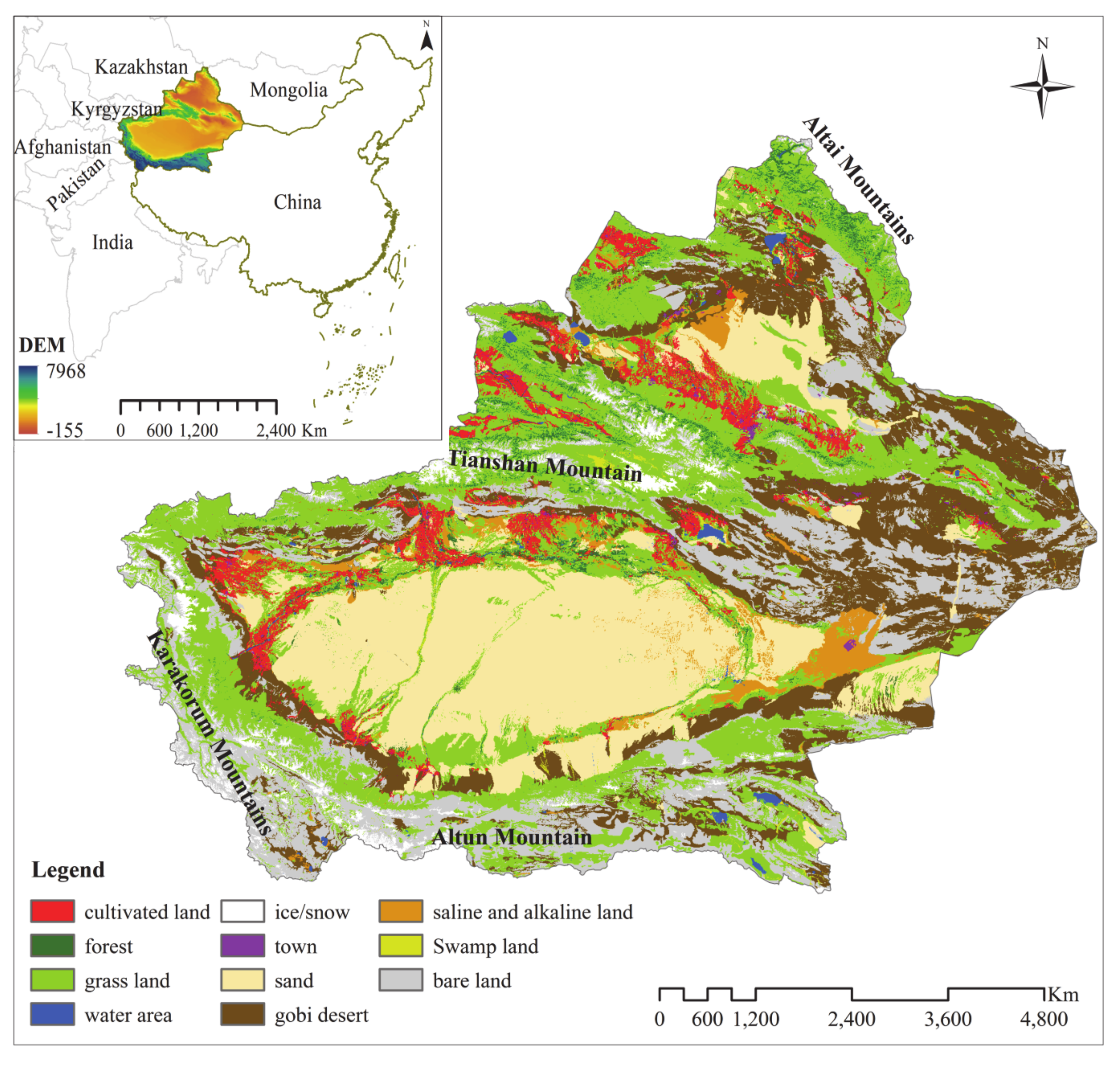
In this study, the ecosystem resilience of the Xinjiang region, located in the arid inland region of Central Asia, was evaluated. The Xinjiang region covers about 1.6 million km² and borders with Mongolia, Russia, Kazakhstan, Kyrgyzstan, Tajikistan, Afghanistan, Pakistan, and India. The most well-known historical route, the Silk Road, ran through the eastern territories towards its northwestern borders. The study area is bounded by the Altai and the Kunlun (Karakorum) Mountains on the northern and southern borders, respectively (Figure 1). The Tianshan Mountains are located in the middle of Xinjiang. It divides Xinjiang into two major basins, the Junggar Basin and the Tarim Basin. According to meteorological data from national meteorological stations of the study area, from 1960 to 2018, Xinjiang has a typical continental arid climate. Annual temperature varies from 10 °C to 13 °C, and annual precipitation varies from 20 mm to 100 mm in the southern parts and from 100 mm to 500 mm in the northern parts of the study area. Land cover is predominantly desert, including sand (21.16%), the Gobi Desert (17.48%), and bare land (18.83%). Forests, grasslands, and farming land account for 2.26%, 28.61%, and 4.72% of the total study area, respectively.

2.2. Data

The MODIS land surface temperature (LST) data (MOD11A2 level data; from 2000 to 2018), normalized difference vegetation index (NDVI; MOD13A1; from 2000 to 2018), and surface albedo data (MCD43B3; from 2000 to2018) were acquired from the National Aeronautics and Space Administration website [28]. The temporal and spatial resolutions of the LST and albedo data are 8 days and 1 × 1 km, respectively. The temporal and spatial resolutions of the NDVI data are 16 days and 500 × 500 m, respectively. The MODIS data were processed using the MODIS reprojection tool to generate a tagged image file format in the WGS84 coordinate system. The study area’s digital elevation model (DEM) was downloaded from the U.S. Geological Survey website [29]. In this study, the LST and albedo data were reprocessed in ArcGIS v10.3 to a spatial resolution of 500 m.

A dataset containing daily mean, maximum, and minimum air temperatures, wind speed, relative humidity, precipitation, mean atmospheric pressure, and sunshine duration data from 68 national meteorological stations from 2000 to 2018 was used [30]. These data were strictly quality-controlled by eliminating missing, erroneous, and suspicious data and other data that had not been quality-controlled. There are 13 vegetation types in the study area as follows: alpine cushion vegetation (ACV), forest (F), shrub (Sh), meadow (M), alpine meadow (AM), alpine steppe (AS), meadow steppe (MS), typical steppe (TS), desert steppe (DS), alpine desert (AD), warm desert (WD), marshland (Mh), and artificial vegetation (cultivated land; CL) [31].

2.3. Methods

We assumed that ecosystems aim to reach maximum biomass, and thus, ecosystem resilience can be regarded as the system’s inherent ability to maintain stability and maximize its biomass. To develop a multi-dimensional ecosystem resilience index, we accounted for three essential aspects of resilience: latitude of resilience, recovery time rate, and resistance. Index development was based on net primary productivity (NPP), assessed using the Carnegie-Ames-Stanford Approach (CASA) model [32,33]. The NPP data calculated in this study have been verified to be reliable [34].

2.3.1. Latitude of Resilience

For a flexible system that is in a regime-stable state, latitude of resilience is the system’s maximum deviation (deviation from the center or mean level). For ecosystems, this can be expressed as follows in Equation (1):

$$LAT=\frac{1}{n}{\displaystyle \sum \max \left|\raisebox{1ex}{${{\displaystyle (NPP}}_{\mathrm{ni}}-{\overline{NPP}}_n)$}\!\left/ \!\raisebox{-1ex}{${{\displaystyle \overline{NPP}}}_n$}\right.\right|}$$

(1)

where n is the number of stages of regime-shift of annual NPP, which is determined using Mann–Kendall tests on annual NPP time series, e.g., for a pixel, in the 2000–2018 period, if there is a regime-shift (significant increase or decrease) in NPP, the annual NPP has two regime-stable (insignificant increase or decrease) stages and thus n = 2; if there is no regime-shift then n = 1. NPP_ni is the annual NPP during a regime-stable stage, while the ${\overline{NPP}}_{\mathrm{n}}$ represents the multiyear mean NPP in the regime-stable stage.

2.3.2. Resistance

This study defined resistance based on sensitivity. The greater the coefficient of sensitivity, the lower the ecosystem resistance to disturbance, within an inverse relationship between sensitivity and resistance. The sensitivity coefficient was calculated as follows in Equation (2):

$${{\displaystyle \epsilon }}_i=\frac{\partial f}{\partial x}\times \frac{\overline{{{\displaystyle x}}_i}}{LUE}$$

(2)

where, ε_i is the sensitivity coefficient of NPP to environmental factors (temperature and precipitation) Xi, at the same time period; and f denotes the function between NPP and X_i. The CASA model can estimate the NPP as follows in Equations (3) and (4):

$$NPP=APAR\times LUE$$

(3)

$$LUE={{\displaystyle T}}_{\epsilon 1}\times {{\displaystyle T}}_{\epsilon 2}\times {{\displaystyle W}}_{\epsilon }\times {{\displaystyle LUE}}_{\max }$$

(4)

where, APAR is the photosynthetically active radiation absorbed by vegetation; T_ε1 and T_ε2 are temperature stress coefficients; W_ε is the water stress coefficient (the ratio of evapotranspiration to potential evaporation); and LUE_max is the maximum light using efficiency. Temperature is directly calculated in Equation (3), but precipitation is not calculated. Precipitation is indirectly determined using the water stress coefficient W_ε and the influence of evapotranspiration. Thus, we constructed the fitting formula between precipitation (p)/temperature (T) and W_ε using the CASA model Equation (5):

$${{\displaystyle W}}_{\epsilon }=0.004p-0.0092T+0.7073$$

(5)

By substituting Equation (4) into (3), the final function between NPP and the climate variables X_i can be obtained. Considering the inverse relationship between sensitivity and resistance, the sensitivity coefficient was standardized to get the resistance index as follows in Equation (6):

$${{\displaystyle R}}_i=\raisebox{1ex}{$\left({{\displaystyle \epsilon }}_{\max }-{{\displaystyle \epsilon }}_{ij}\right)$}\!\left/ \!\raisebox{-1ex}{$\left({{\displaystyle \epsilon }}_{\max }-{{\displaystyle \epsilon }}_{\min }\right)$}\right.$$

(6)

Thus, the resistance coefficients R_t and R_p, which are the ecosystem’s resistance coefficients to temperature and precipitation, respectively, were estimated.

2.3.3. Recovery Time Rate

Recovery rate is defined as the time required for an ecosystem to return to equilibrium state after being disturbed. Larger recovery rates mean less time to recover after disturbance. In our framework, recovery rate was calculated as follows in Equation (7):

$$C=\frac{1}{m}{\displaystyle {\sum }_{i=1}^m\frac{\left|\left(\overline{{{\displaystyle NPP}}_{\mathrm{m}}}-\overline{NPP}\right)\right|}{{{\displaystyle \mathrm{t}}}_m}}$$

(7)

where, C is the average recovery time of the system to return from ‘deviation’ due to disturbance, to the multi-year average; m is the number of data segments greater or less than the multi-year average $NPP$; ${\overline{NPP}}_m$ is the mean $NPP$ of the data segments m; $\overline{NPP}$ is the mean $NPP$ of the total $NPP$ time series data; and tm is the number of years covered by the m data segments. To eliminate the influence of different units, the data were standardized as follows in Equation (8):

$$Rec=\raisebox{1ex}{$\left({{\displaystyle C}}_i-{{\displaystyle C}}_{\min }\right)$}\!\left/ \!\raisebox{-1ex}{$\left({{\displaystyle C}}_{\max }-{{\displaystyle C}}_{\min }\right)$}\right.$$

(8)

where, C_i is the average recovery time in pixel i, while C_max and C_min are the maximum and minimum values of the average recovery time in the entire region. The recovery time rate (Rec) index ranged from 0 to 1, with larger values denoting higher recovery time rates.

2.3.4. Comprehensive Resilience Index

Considering the multi aspects of resilience, this study proposed a comprehensive ecosystem resilience index and is calculated as follows in Equation (9):

$$RSL=\raisebox{1ex}{$\left(LAT+Rec+{{\displaystyle R}}_p+{{\displaystyle R}}_t\right)$}\!\left/ \!\raisebox{-1ex}{$4$}\right.$$

(9)

2.3.5. Grading of Resilience Indicators

Although we propose a simple multi-dimensional index of ecosystem resilience, we often need to classify the quantitative indices into different ecosystem-management or decision-support classes. Such levels are resilient, slightly nonresilient, moderately nonresilient, and severely nonresilient. Because of the lack of a grading scheme, we referred to existing research and used ArcGIS (V10.3) to develop a comprehensive resilience index grading system based on the natural break method [26].

3. Results

3.1. Multidimensional Characters of Resilience

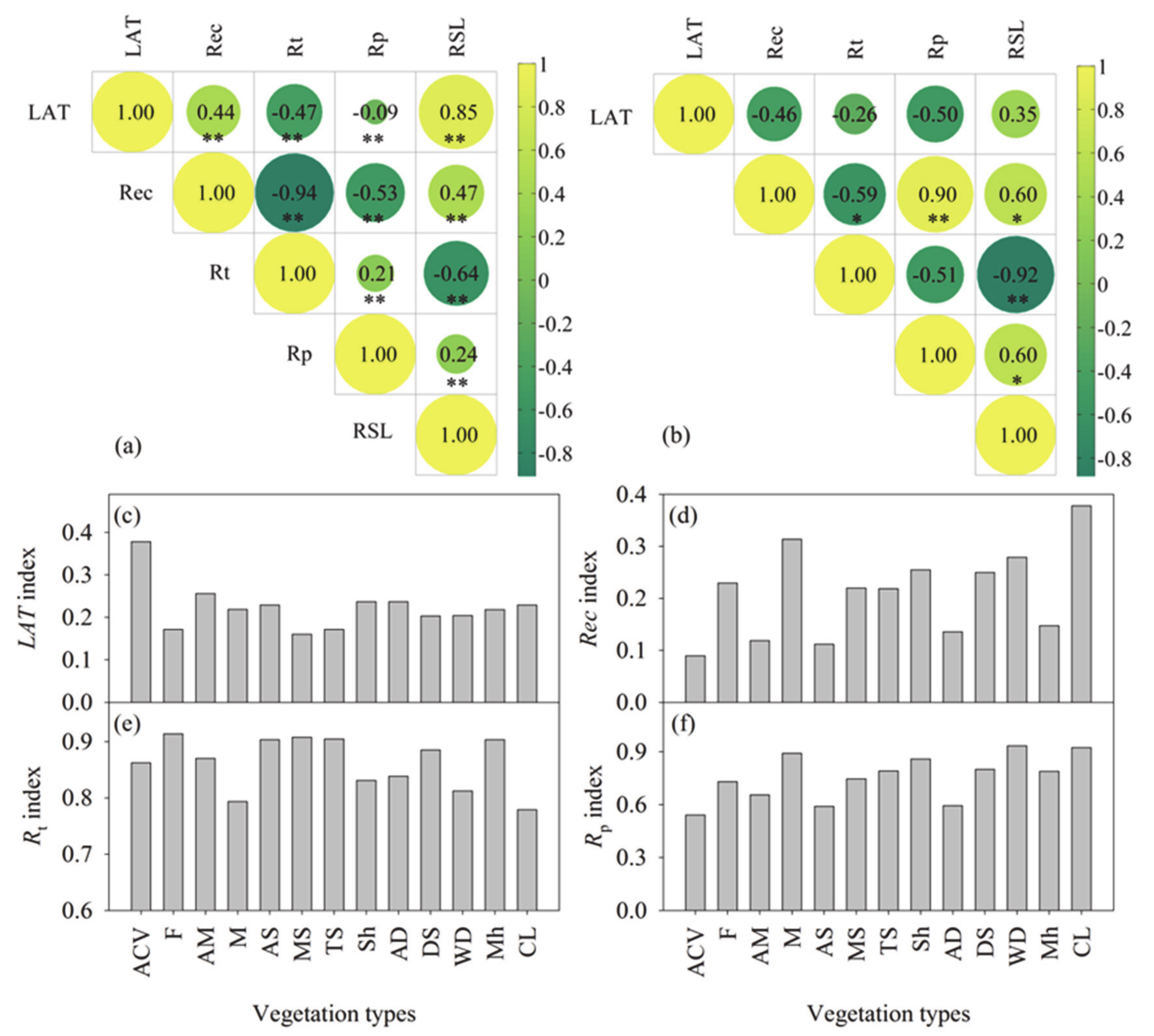
The multidimensional characteristics of resilience, including latitude of resilience (LAT), recovery time rate (Rec), and resistance to temperature (R_t) and precipitation (R_p), showed a significant correlation with each other (Figure 2). On the pixel scale (Figure 2a), the LAT index was positively correlated with the Rec index, while it was negatively correlated with the resistance index, that is, R_t and R_p. The Rec index was negatively correlated with the resistance index. As for the two resistance indices, there was a positive correlation between R_t and R_p. The results show that for an ecosystem, more robust resistance to disturbance is often also combined with lower latitude of resilience and recovery time rate. Regarding vegetation types (Figure 2b), only the Rec index was significantly correlated with R_t and R_p. Thus, a single index, such as the resistance index or LAT, R_t, and R_p. Thus, a single index, such as the resistance index or LAT index, could not reflect the real status of ecosystem resilience. Given this, this study suggests the use of the comprehensive resilience indicator (RSL). The RSL index was significantly correlated with all four sub-indices on the scale of pixel vegetation types. The assessment results of ecosystem resilience on the vegetation types showed apparent variability (Figure 2c–f). Alpine cushion vegetation has the highest latitude of resilience, but it also has the lowest recovery rate and resistance to precipitation. As for the warm desert, although it has the highest resistance to precipitation and a higher recovery rate, it also has a lower resistance to temperature. Obviously, there is great uncertainty in using a single indicator to evaluate ecosystem resilience, mainly due to the inconsistency of the evaluation perspective and the multi-dimensional nature of ecosystem resilience.

3.2. Comprehensive Resilience

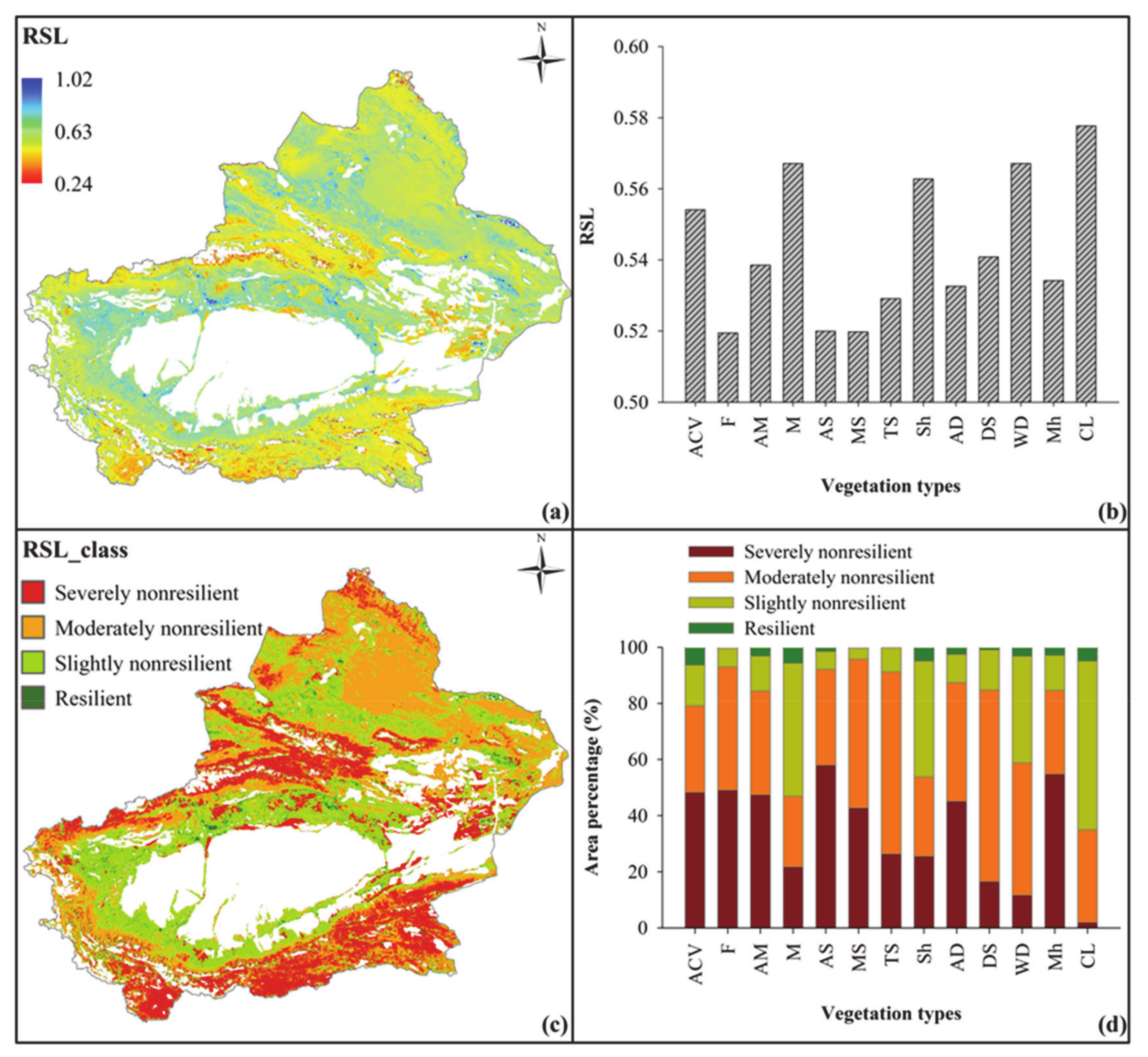
Based on the variability of the four aspects of resilience, the comprehensive resilience index (RSL) was adopted to represent the state of ecosystem resilience (Figure 3). The spatial variability of the RSL index ranged from 0.24 to 1.02; ecosystem resilience of the oasis area was the highest, with an average value of 0.58 followed by plain desert area (0.56) and mountain area, which was the lowest, with an average value of 0.52. For the different vegetation types, ecosystem resilience of artificial vegetation (crop land) had the highest resilience, and the RSL index was 0.58. In contrast, forest had the lowest resilience (0.52). Generally, warm desert, meadow, and shrubs have higher resilience, while alpine and meadow steppes have lower resilience (Figure 3a,b).

This study used the natural break method to categorize the comprehensive ecosystem resilience into four classes: resilient (RSL ≥ 1.02), slightly nonresilient (0.64 ≤ RSL < 1.01), moderately nonresilient (0.56 ≤ RSL < 0.64) and severely nonresilient (RSL < 0.56). The results showed that the study area was mainly dominated by moderately and slightly nonresilient areas. In the oasis, plain desert, and mountain areas, the resilient area only accounted for 4.93%, 4.24%, and 2.35% of their total areas. Simultaneously, the sum of the slightly and moderately nonresilient areas accounted for 93.11%, 85.80%, and 59.54% of their total areas. Warm deserts and meadows have high resilience, and the elastic area only accounted for 3.20% and 5.70% of the total area. Meanwhile, the sum of the slightly and moderately nonresilient areas accounted for 85.18% and 72.58% of their total areas. For the alpine and meadow steppes with the poor resilience, the severely resilient areas account for 57.95% and 42.72% of their total areas, respectively. In general, the area percentage of the nonresilient area (Figure 3d) of different vegetation types was negatively correlated with the changing trend of comprehensive resilience of them (R² = 0.56).

3.3. Coverage, NPP, and Resilience

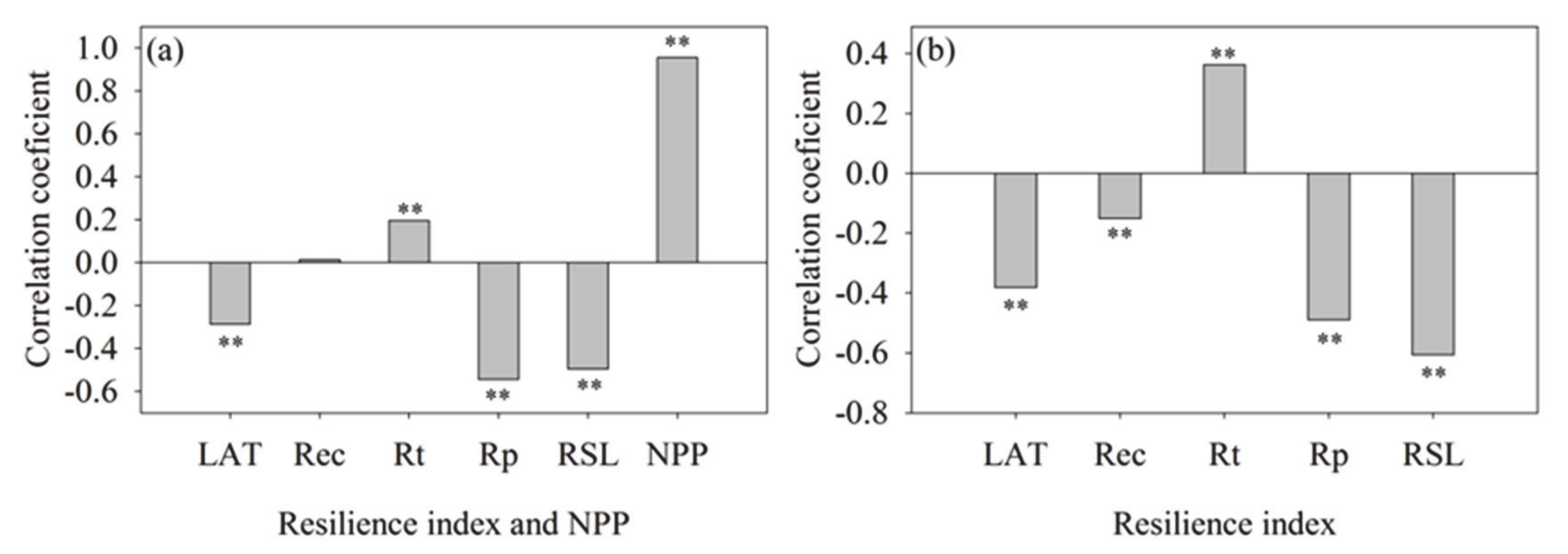
Generally, vegetation with profitable growth and high coverage often means that the ecosystem may have high diversity and ecosystem stability, but this does not mean high ecosystem resilience. At least in arid areas, this view needs to be updated. This study showed that the resilience index, except the Rec, all presented a significant correlation with vegetation coverage. Among them, the LAT, R_p, and RSL index were negatively correlated with vegetation coverage, and the correlation coefficients was −0.29, −0.54, and −0.50, respectively, while the R_t index was positively correlated with coverage, and the correlation coefficient was 0.20 (Figure 4a). Although the higher vegetation coverage can bring higher biomass (correlation coefficient was 0.96), the higher biomass was not equivalent to the high ecosystem resilience (Figure 4a,b). Similarly, the LAT, R_p, and RSL index were also significantly negatively correlated with NPP, and the correlation coefficients were −0.38, −0.49, and −0.61, respectively.

4. Discussion

4.1. The Improvement and Reliability of the Method

Ecosystem resilience is an important characteristic of ecosystems that reflects their health. Thus, accurate assessment of ecosystem resilience is vital for sustainable ecosystem management [35,36]. Currently, there are three simple, effective methods to assess ecosystem resilience at large scales based on: (1) ecosystem water-use efficiency (WUE) [26]; (2) vegetation and climate anomalies (VCA) [27]; and (3) methods based on regime shift of NDVI time-series data.

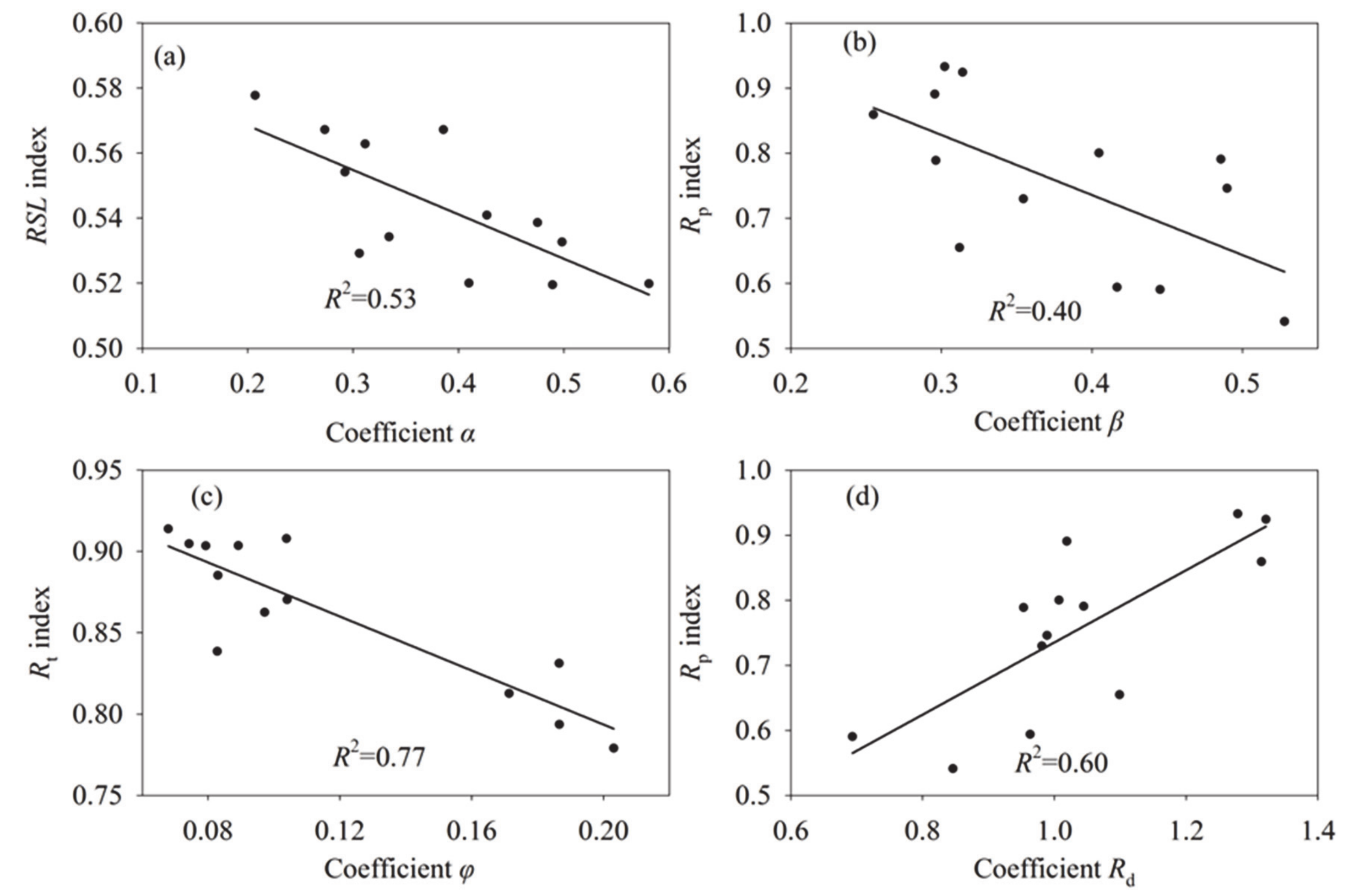
Although the new index we proposed has advantages, the accuracy-reliability of the index needs to be further verified. In this study, the original method’s results were compared with those calculated based on the on the WUE (Appendix A) and VCA (Appendix B) methods, respectively. In WUE-based calculations, the ratio of WUE in the driest year to the mean WUE of the entire period was defined as the R_d coefficient, denoting the ecosystem’s resistance to drought, and the more extensive R_d indicating higher resilience [26]. In the VCA method, three key coefficients of the model, namely α, β, and ϕ, can be calculated. Coefficient α reflects the resilience of the ecosystem, with larger values indicating a low resilience. At the same time, β and ϕ represent the drought-resistance and temperature-resistance metrics, respectively. Larger β and ϕ values indicate low resistance [27].

The comparison results showed that the RSL index was negatively correlated with coefficient α, while the R_t and R_w indexes were also negatively correlated with coefficients ϕ and β, respectively (Figure 5). Additionally, coefficient R_d was negatively correlated with coefficient β, while it was positively correlated with R_w. The above comparative analysis showed that although there are differences in the index values calculated by the method proposed in this study and existing methods, all indices had consistent trends. The results suggest that this method-index can replace current methods in most cases, and it is also a useful supplement and improvement of the existing ecosystem resilience assessments.

4.2. Resistance, Resilience, and the Stability

In ecosystem resilience assessments, the resistance index is often regarded as a critical variable reflecting resilience [10,13]. Studies evaluate the resilience of ecosystems, mainly by employing the resistance index [21,26]. Our study confirmed that ecosystem resistance was positively correlated with the RSL index, and the contribution rate of R_t and R_w to RSL was 35.74% and 36.13%, respectively, which was more than 2 and 3 times that of the LAT and Rec indices.

We also found that high coverage does not always reflect high ecosystem resilience. In this study, resilience had a decreasing trend with the increase of vegetation coverage (Figure 4). The reason may be that ecosystems with low vegetation coverage, such as warm deserts, tend to have more significant biomass fluctuations. Hence, the LAT index is broader, and the recovery rate is faster (Figure 2c,d). Simultaneously, low vegetation coverage also has higher resistance, and the resistance almost dominates the overall resilience calculations. Thus, low vegetation coverage leads to high resistance probably because the vegetation system is always fluctuating due to environmental disturbance, being like an elastomeric. On the contrary, bare land is like a rigid body, which has little response to environmental change. Therefore, ecosystems with low vegetation coverage, i.e., large bare lands, usually have low sensitivity to environmental change and thus higher resistance.

But does low resilience also mean low stability? Here we need to distinguish between two very confusing concepts: ecosystem stability and resilience. Initially, ecosystem resilience is focused on ecosystem recovery time rate after disturbances (recovery or engineering resilience) [16]. The stability of an ecosystem includes resilience and resistance, usually in inverse proportion. Our study confirmed that the LAT and Rec indices were significantly negatively correlated with the R_t and R_p indices (Figure 2a,b). Then, after deepening our understanding of resilience, the concept of ecosystem resilience was further expanded. Recently, ecosystem resilience encompasses aspects of both recovery and resistance [12,18,19,20]. Furthermore, the latitude of resilience is also an essential metric of ecosystem resilience [37]. Therefore, ecosystem resilience is a crucial aspect of ecosystem stability but it cannot fully represent its stability. In some cases, ecosystem resilience cannot effectively reflect fluctuations of ecosystem stability caused by diversity variability [21]. The results of this study suggest that in the arid desert area, desert vegetation has a home-field advantage, and thus it is not surprising that it has strong resilience. On the contrary, as nonzonal vegetation, the mountain forest is mainly composed of single spruce species and has lower diversity than the zonal forest area. Thus, it has lower resilience.

4.3. Ecosystem Resilience and Ecosystem Management

Our study area is the driest region in China, where the observed rise rate of temperature reached 0.32–0.35 °C/10a [38,39]. With increased temperature, precipitation also indicates a significant increasing trend in the study area [40]. Obviously, climate change has profound impacts on the water cycle and ecosystem stability of arid regions [41,42,43,44,45]. Under the impacts of climate change and anthropogenic activities, the stability of arid ecosystems is greatly affected. Thus, we propose that targeted management measures should be applied based on ecosystem resilience. Ecological restoration in ecosystems of low resilience or severe damage may be of first priority to maintain ecosystem stability. Although resilience is almost uniformly used in the ecosystem-management literature to refer to the ability of ecosystems to resist transition to alternative states or recover without intervention, resilience, in reality, is a positive or a negative property of ecosystems depending on their state of degradation [13]. Thus, distinguishing between helpful and unhelpful resilience is an essential step in ecosystem management. In this study, warm deserts, meadows, and shrubs have high resilience (Figure 3), which can help them maintain stability; thus we do not need to carry out additional human interventions for these ecosystems if catastrophic disturbance is not present. In contrast, for forests, the RSL index is low. Among them, the proportion of slightly nonresilient and resilient areas is small, and the average value is also small. Once the forest is undergoing a retrograde succession into shrubs or grassland (their resilience is higher than forest), we need to overcome the useless resilience. The cost of ecological restoration is much higher than the original cost of maintaining the ecological environment. We should pay attention to human intervention to prevent ecosystem degradation. Similarly, we should also focus management on alpine steppes, typical steppes, and desert steppes, and if necessary, apply timely artificial interventions to prevent the reverse succession of them.

5. Conclusions

This study proposed a comprehensive resilience assessment index encompassing four aspects of ecosystem resilience: latitude of ecosystem resilience, recovery time rate after disturbance, and resistance to temperature and precipitation based on the CASA model and NPP data. The index was applied to evaluate the resilience of typical arid ecosystems in Central Asia, and the results were consistent with existing results, indicating that the results of this new method are reliable. As a step forward, this method considered representative indices of three dimensions of ecosystem resilience, effectively avoiding the uncertainty of previous results that were based on single or limited dimension indices. There was no consistent positive correlation among indices, which suggests that the use of a single index to evaluate resilience would result in great uncertainty. Thus, applying a comprehensive resilience index is a more accurate approach to such problems. Ecosystem resilience of the study area was generally low, dominated by slightly and moderately nonresilient areas. High vegetation coverage and biomass do not always bring high resilience. Overall, this method is based on the CASA model and has a specific physical basis rather than a single statistical analysis. Simultaneously, it is easy to apply and can be used to evaluate and compare the resilience from pixel to vegetation type or watershed (region) scales. In general, this method/index is a useful supplement and improvement for ecosystem resilience assessments research.

References

- Craine, J.M.; Ocheltree, T.W.; Nippert, J.B.; Towne, E.G.; Skibbe, A.M.; Kembel, S.W.; Fargione, J.E. Global diversity of drought tolerance and grassland climate-change resilience. Nat. Clim. Chang. 2012, 3, 63–67. [Google Scholar] [CrossRef]
- Marx, A.; Erhard, M.; Thober, S.; Kumar, R.; Shafer, D.; Samaniego, L.; Zink, M. Climate Change as Driver for Ecosystem Services Risk and Opportunities, in Atlas of Ecosystem Services: Drivers, Risks, and Societal Responses; Springer: Berlin/Heidelberg, Germany, 2019; pp. 173–178. [Google Scholar]
- Schirpke, U.; Kohler, M.; Leitinger, G.; Fontana, V.; Tasser, E.; Tappeiner, U. Future impacts of changing land-use and climate on ecosystem services of mountain grassland and their resil-ience. Ecosyst. Serv. 2017, 26, 79–94. [Google Scholar] [CrossRef]
- Holl, K.; Aide, T. When and where to actively restore ecosystems? For. Ecol. Manag. 2011, 261, 1558–1563. [Google Scholar] [CrossRef]
- Moritz, C.; Agudo, R. The Future of Species under Climate Change: Resilience or Decline? Science 2013, 341, 504–508. [Google Scholar] [CrossRef] [PubMed]
- Valdecantos, A.; Baeza, M.J.; Vallejo, V.R. Vegetation Management for Promoting Ecosystem Resilience in Fire-Prone Med-iterranean Shrublands. Restor. Ecol. 2008, 17, 414–421. [Google Scholar] [CrossRef]
- Johnson, R.M.; Edwards, E.; Gardner, J.S.; Diduck, A.P. Community vulnerability and resilience in disaster risk reduction: An example from Phojal Nalla, Himachal Pradesh, India. Reg. Environ. Chang. 2018, 18, 2073–2087. [Google Scholar] [CrossRef] [Green Version]
- Peng, M.; Wen, Z.; Xie, L.; Cheng, J.; Jia, Z.; Shi, D.; Zeng, H.; Zhao, B.; Liang, Z.; Li, T.; et al. 3D Printing of Ultralight Biomimetic Hierarchical Graphene Materials with Exceptional Stiffness and Resilience. Adv. Mater. 2019, 31, e1902930. [Google Scholar] [CrossRef]
- Stork, N.; Coddington, J.A.; Colwell, R.K.; Chazdon, R.L.; Dick, C.W.; Peres, C.A.; Sloan, S.; Willis, K. Vulnerability and Resilience of Tropical Forest Species to Land-Use Change. Conserv. Biol. 2009, 23, 1438–1447. [Google Scholar] [CrossRef]
- Connell, S.D.; Ghedini, G. Resisting regime-shifts: The stabilising effect of compensatory processes. Trends Ecol. Evol. 2015, 30, 513–515. [Google Scholar] [CrossRef]
- Holling, C.S. Resilience and Stability of Ecological Systems. Annu. Rev. Ecol. Syst. 1973, 4, 1–23. [Google Scholar] [CrossRef] [Green Version]
- Hodgson, D.; McDonald, J.L.; Hosken, D.J. What do you mean, ‘resilient’? Trends Ecol. Evol. 2015, 503–506. [Google Scholar] [CrossRef] [PubMed]
- Standish, R.J.; Hobbs, R.J.; Mayfield, M.M.; Bestelmeyer, B.T.; Suding, K.N.; Battaglia, L.L.; Eviner, V.T.; Hawkes, C.V.; Temperton, V.M.; Cramer, V.A.; et al. Resilience in ecology: Abstraction, distraction, or where the action is? Biol. Conserv. 2014, 177, 43–51. [Google Scholar] [CrossRef] [Green Version]
- Yeung, A.C.; Richardson, J.S. Some Conceptual and Operational Considerations when Measuring ‘Resilience’: A Response to Hodgson et al. Trends Ecol. Evol. 2016, 31, 2–3. [Google Scholar] [CrossRef] [PubMed] [Green Version]
- Vogel, A.; Scherer-Lorenzen, M.; Weigelt, A. Grassland Resistance and Resilience after Drought Depends on Management Intensity and Species Richness. PLoS ONE 2012, 7, e36992. [Google Scholar] [CrossRef]
- Pimm, S.L. The complexity and stability of ecosystems. Nat. Cell Biol. 1984, 307, 321–326. [Google Scholar] [CrossRef]
- Sasaki, T.; Furukawa, T.; Iwasaki, Y.; Seto, M.; Mori, A.S. Perspectives for ecosystem management based on ecosystem resilience and ecological thresholds against multiple and stochastic disturbances. Ecol. Indic. 2015, 57, 395–408. [Google Scholar] [CrossRef]
- Côté, I.M.; Darling, E.S. Rethinking Ecosystem Resilience in the Face of Climate Change. PLoS Biol. 2010, 8, e1000438. [Google Scholar] [CrossRef]
- McClanahan, T.R.; Donner, S.D.; Maynard, J.A.; MacNeil, M.A.; Graham, N.A.; Maina, J.; Baker, A.C.; Beger, A.C.; Beger, M.; Campbell, S.J.; et al. Prioritizing Key Resilience Indicators to Support Coral Reef Management in a Changing Climate. PLoS ONE 2012, 7, e42884. [Google Scholar] [CrossRef]
- Oliver, T.H.; Heard, M.S.; Isaac, N.J.; Roy, D.B.; Procter, D.A.; Eigenbrod, F.; Freckleton, R.P.; Hector, A.; Orme, C.D.L.; Petchey, O.L.; et al. Biodiversity and Resilience of Ecosystem Functions. Trends Ecol. Evol. 2015, 30, 673–684. [Google Scholar] [CrossRef] [Green Version]
- Walker, B.; Holling, C.S.; Carpenter, S.R.; Kinzig, A.P. Resilience, Adaptability and Transformability in Social-ecological Systems. Ecol. Soc. 2004, 9, 3438–3447. [Google Scholar] [CrossRef]
- Mouillot, D.; Graham, N.A.J.; Villéger, S.; Mason, N.W.H.; Bellwood, D.R. A functional approach reveals community responses to disturbances. Trends Ecol. Evol. 2013, 28, 167–177. [Google Scholar] [CrossRef] [PubMed]
- Briske, D.D.; Fuhlendorf, S.D.; Smeins, F.E. State-and-Transition Models, Thresholds, and Rangeland Health: A Synthesis of Ecological Concepts and Perspectives. Rangel. Ecol. Manag. 2005, 58, 1–10. [Google Scholar] [CrossRef]
- Meyer, K.; Hoyer-Leitzel, A.; Iams, S.; Klasky, I.; Lee, V.; Ligtenberg, S.; Bussmann, E.; Zeeman, M.L. Quantifying resilience to recurrent ecosystem disturbances using flow–kick dynamics. Nat. Sustain. 2018, 1, 671–678. [Google Scholar] [CrossRef]
- Campos, G.E.; Moran, S.M.; Huete, A.; Zhang, Y.; Bresloff, S.; Huxman, T.E.; Eamus, E.; Bosch, D.D.; Buda, A.R.; Gunter, S.A.; et al. Ecosystem resilience despite large-scale altered hydroclimatic conditions. Nature 2013, 494, 349–352. [Google Scholar] [CrossRef] [PubMed]
- Sharma, A.; Goyal, M.K. Assessment of ecosystem resilience to hydroclimatic disturbances in India. Glob. Chang. Biol. 2018, 24, e432–e441. [Google Scholar] [CrossRef]
- De Keersmaecker, W.; Lhermitte, S.; Tits, L.; Honnay, O.; Somers, B.; Coppin, P. A model quantifying global vegetation resistance and resilience to short-term climate anomalies and their relationship with vegetation cover. Glob. Ecol. Biogeogr. 2015, 24, 539–548. [Google Scholar] [CrossRef]
- MODIS. Available online: http://modis.gsfc.nasa.gov/ (accessed on 1 November 2019).
- USGS. Available online: http://tahoe.usgs.gov/DEM.html (accessed on 1 November 2019).
- CMDC. Available online: http://data.cma.cn/data/cdcdetail/dataCode/SURF_CLI_CHN_MUL_DAY_V3.0.html (accessed on 1 November 2019).
- REDCP, CAS. Available online: http://www.resdc.cn (accessed on 1 November 2019).
- Sannigrahi, S. Modeling terrestrial ecosystem productivity of an estuarine ecosystem in the Sundarban Biosphere Region, India using seven ecosystem models. Ecol. Model. 2017, 356, 73–90. [Google Scholar] [CrossRef]
- Piao, S.; Fang, J.; Zhou, L.; Zhu, B.; Tan, K.; Tao, S. Changes in vegetation net primary productivity from 1982 to 1999 in China. Glob. Biogeochem. Cycles 2005, 19. [Google Scholar] [CrossRef] [Green Version]
- Hao, X.; Ma, H.; Hua, D.; Qin, J.; Zhang, Y. Response of ecosystem water use efficiency to climate change in the Tianshan Mountains, Central Asia. Environ. Monit. Assess. 2019, 191, 561. [Google Scholar] [CrossRef]
- Saroar, M.; Rahman, M. Ecosystem-Based Adaptation: Opportunities and Challenges in Coastal Bangladesh: Policy Strategies for Adaptation and Resilience. In The Anthropocene: Politik Economics Society Science; Springer: Cham, Switzerland, 2019; Volume 28. [Google Scholar] [CrossRef]
- Lam, V.Y.Y.; Doropoulos, C.; Mumby, P.J. The influence of resilience-based management on coral reef monitoring: A systematic review. PLoS ONE 2017, 12, e0172064. [Google Scholar] [CrossRef]
- Fatemeh, H.; Reza, J.; Hossein, B.; Mostafa, T.; Kenneth, C.D. Estimation of spatial and temporal changes in net primary production based on Carnegie Ames Stanford Ap-proach(CASA) model in semi-arid rangelands of Semirom County, Iran. J. Arid Land 2019, 477–494. [Google Scholar]
- Jiang, Y.A.; Chen, Y.; Zhao, Y.Z.; Chen, P.X.; Yu, X.J.; Fan, J.; Bai, S.Q. Analysis on Changes of Basic Climatic Elements and Extreme Events in Xinjiang, China during 1961–2010. Adv. Clim. Chang. Res. 2013, 4, 20–29. [Google Scholar] [CrossRef]
- Xu, C.; Li, J.; Zhao, J.; Gao, S.; Chen, Y. Climate variations in northern Xinjiang of China over the past 50 years under global warming. Quat. Int. 2015, 358, 83–92. [Google Scholar] [CrossRef]
- Wang, H.; Chen, Y.; Chen, Z. Spatial distribution and temporal trends of mean precipitation and extremes in the arid region, northwest of China, during 1960–2010. Hydrol. Process. 2012, 27, 1807–1818. [Google Scholar] [CrossRef]
- Kundzewicz, Z.W. Climate change impacts on the hydrological cycle. Ecohydrol. Hydrobiol. 2008, 8, 195–203. [Google Scholar] [CrossRef] [Green Version]
- Sun, S.; Sun, G.; Cohen, E.; McNulty, S.G.; Caldwell, P.V.; Duan, K.; Zhang, Y. Projecting water yield and ecosystem productivity across the United States by linking an ecohydrological model to WRF dynamically downscaled climate data. Hydrol. Earth Syst. Sci. 2016, 20, 935–952. [Google Scholar] [CrossRef] [Green Version]
- Sorg, A.; Bolch, T.; Stoffel, M.; Solomina, O.; Beniston, M. Climate change impacts on glaciers and runoff in Tien Shan (Central Asia). Nat. Clim. Chang. 2012, 2, 725–731. [Google Scholar] [CrossRef]
- Etemadi, H.; Samadi, S.; Sharifikia, M.; Smoak, J.M. Assessment of climate change downscaling and non-stationarity on the spatial pattern of a mangrove ecosystem in an arid coastal region of southern Iran. Theor. Appl. Clim. 2016, 126, 35–49. [Google Scholar] [CrossRef]
- Li, W.; Li, X.; Zhao, Y.; Zheng, S.; Bai, Y. Ecosystem structure, functioning and stability under climate change and grazing in grasslands: Current status and future prospects. Curr. Opin. Environ. Sustain. 2018, 33, 124–135. [Google Scholar] [CrossRef]
- Crabtree, R.; Potter, C.; Mullen, R.; Sheldon, J.; Huang, S.; Harmsen, J.; Rodman, A.; Jean, C. A modeling and spatio-temporal analysis framework for monitoring environmental change using NPP as an ecosystem indicator. Remote Sens. Environ. 2009, 113, 1486–1496. [Google Scholar] [CrossRef] [Green Version]
- Yang, H.; Mu, S.; Li, J. Effects of ecological restoration projects on land use and land cover change and its influences on territorial NPP in Xinjiang, China. Catena 2014, 115, 85–95. [Google Scholar] [CrossRef]
- Allen, R.G.; Irmak, A.; Trezza, R.; Hendrickx, J.M.H.; Bastiaanssen, W.G.M.; Kjaersgaard, J. Satellite-based ET estimation in agriculture using SEBAL and METRIC. Hydrol. Process. 2011, 25, 4011–4027. [Google Scholar] [CrossRef]
- Tegos, A.; Malamos, N.; Koutsoyiannis, D. A parsimonious regional parametric evapotranspiration model based on a sim-plification of the Penman–Monteith formula. J. Hydrol. 2015, 524, 708–717. [Google Scholar] [CrossRef]
Figure 1.
Xinjiang region geographical location, topography, and land use: geographical location data from standard map website (Review picture serial number: GS(2019)3266), The DEM data are from USGS, and the land use types are abbreviated from the vegetation type map of China at a scale of 1:1,000,000.
Figure 2.
The correlation between the index of different aspects of ecosystem resilience and their values on different vegetation types: (a,b) are the correlation of each index on the scale of pixel and vegetation type, respectively. The symbol ‘**’ and ‘*’ in (a,b) indicates the extremely significant correlation and significant correlation, respectively. Panel (c–f) shows the latitude of resilience (LAT), recovery rate (Rec), and the resistance of ecosystem to temperature (Rt) and precipitation (Rp) on vegetation type scale. ACV stands for alpine cushion vegetation, F stands for forest, Sh stands for shrub, M stands for meadow, AM stands for alpine meadow, AS stands for alpine steppe, MS stands for meadow steppe, TS stands for typical steppe, DS stands for desert steppe, AD stands for alpine desert, WD stands for warm desert, Mh stands for marshland, and CL stands for cultivated land.
Figure 3.
The comprehensive ecosystem resilience (RSL) index in the study region. (a) RSL on the pixel scale, (b) average RSL of different vegetation types, (c) the grading results of RSL, and (d) area percentage of different RSL classifications for different vegetation types. In (b,d), ACV stands for alpine cushion vegetation, F stands for forest, Sh stands for shrub, M stands for meadow, AM stands for alpine meadow, AS stands for alpine steppe, MS stands for meadow steppe, TS stands for typical steppe, DS stands for desert steppe, AD stands for alpine desert, WD stands for warm desert, Mh stands for marshland, and CL stands for cultivated land.
Figure 4.
Correlation analysis between mean coverage, resilience index, and NPP on vegetation type scales. (a) Is the correlation between mean resilience index, NPP, and vegetation coverage of different vegetation types. (b) Is the correlation between mean NPP and resilience index of different vegetation types. ‘**’ indicates the extremely significant correlation between them.
Figure 5.
Scatter plot between the resilience index of the new method that proposed by this study and that of the existing methods. (d) The coefficient of Rd is the resilience index that calculated by the method which based on the ecosystem water use efficiency. (a–c) Coefficient α, β, and φ was the resilience and resistance index that calculated by the method which based on the annual NDVI and climatic factors (including temperature and drought index) anomalies. (a) The coefficient α represents system returns to equilibrium, with large values indicates a low resilience. (b,c) While the coefficients β and φ represents the drought-resistance and temperature-resistance metrics, respectively. And the large values of coefficient β and φ indicate a low resistance to droughts/temperature anomalies.
Publisher’s Note: MDPI stays neutral with regard to jurisdictional claims in published maps and institutional affiliations. |
© 2021 by the authors. Licensee MDPI, Basel, Switzerland. This article is an open access article distributed under the terms and conditions of the Creative Commons Attribution (CC BY) license (http://creativecommons.org/licenses/by/4.0/).
Share and Cite
MDPI and ACS Style
Fan, X.; Hao, X.; Hao, H.; Zhang, J.; Li, Y. Comprehensive Assessment Indicator of Ecosystem Resilience in Central Asia. Water 2021, 13, 124. https://doi.org/10.3390/w13020124
AMA Style
Fan X, Hao X, Hao H, Zhang J, Li Y. Comprehensive Assessment Indicator of Ecosystem Resilience in Central Asia. Water. 2021; 13(2):124. https://doi.org/10.3390/w13020124
Chicago/Turabian StyleFan, Xue, Xingming Hao, Haichao Hao, Jingjing Zhang, and Yuanhang Li. 2021. "Comprehensive Assessment Indicator of Ecosystem Resilience in Central Asia" Water 13, no. 2: 124. https://doi.org/10.3390/w13020124
Note that from the first issue of 2016, this journal uses article numbers instead of page numbers. See further details here.