Sectorization for Water Distribution Systems with Multiple Sources: A Performance Indices Comparison

Abstract

Sectorization is an effective technique for reducing the complexities of analyzing and managing of water systems. The resulting sectors, called district metering areas (DMAs), are expected to meet some requirements and performance criteria such as minimum number of intervention, pressure uniformity, similarity of demands, water quality and number of districts. An efficient methodology to achieve all these requirements together and the proper choice of a criteria governing the sectorization is one of the open questions about optimal DMAs design. This question is addressed in this research by highlighting the advantages of three different criteria when applied to real-word water distribution networks (WDNs). To this, here it is presented a two-stage approach for optimal design of DMAs. The first stage, the clustering of the system, is based on a Louvain-type greedy algorithm for the generalized modularity maximization. The second stage, the physical dividing of the system, is stated as a two-objective optimization problem that utilises the SMOSA version of simulated annealing for multiobjective problems. One objective is the number of isolation valves whereas for the second objective three different performance indices (PIs) are analyzed and compared: (a) standard deviation, (b) Gini coefficient and (c) loss of resilience. The methodology is applied to two real case studies where the first two PIs are optimized to address similar demands among DMAs. The results demonstrate that the proposed method is effective for sectorization into independent DMAs with similar demands. Surprisingly, it found that for the real studied systems, loss of resilience achieves better performance for each district in terms of pressure uniformity and demand similarity than the other two specific performance criteria.

1. Introduction

Modern societies critically depend on infrastructure networks. A good example of these are the water distribution networks (WDNs) that are designed for distributing drinking water among consumers. In aged networks, the quality of this service is strongly affected by the growing demand for water in expanding cities and by leaks that occur as a result of the aging of the components of the hydraulic system. Water quality control, leakage reduction and pressure management are difficult tasks due to the size of the water networks and the non-linear nature of the hydraulic system. Partitioning water distribution networks into smaller areas, called district metering areas (DMAs), is an effective technique that reduces the complexities of analyzing and managing these infrastructures.

In the last decade, a growing body of work has shown a wide range of methods for sectorization of water networks (see ref. [1] for a review). Optimal sectorization in a single stage is computationally prohibitive even for middle size networks. This is so because hydraulic constraints must be evaluated for every candidate solution in order to meet a number of requirements that characterize a good WDN partitioning [2]. Inside this context, there is an intense research to find less time consuming methods [3]. In general terms, the design methods follow two-stages. The first stage seeks WDN clustering based on topological considerations and is accomplished by using different concepts of graph theory [2,4,5,6,7,8,9,10], complex network theory [11,12,13,14,15,16,17,18] or multiagent approach [19]. Interesting studies comparing the performance of different partitioning algorithms are given in refs. [20,21]. The second stage deals with the placement of flowmeters and valves based on some PI to be optimized. Several alternatives for these indicators were used in the literature: resilience index [8,22,23], background leakages [16], number of flow observations [12,16] in addition of hydraulic indicators as water age, entropy [8], and dissipated power [5] (see ref. [24] for an improvement of this method). Other frameworks based on the concept of modularity propose the use of fast-greedy partitioning algorithm for creating DMAs through information encoded by pipe weights [25]. Recently and with a more wide perspective, in ref. [26] it is proposed a dynamic partitioning of WDNs for an efficient and sustainable management in response to goals as saving energy, water and monetary costs. In addition, this dynamic DMAs framework has shown to be useful for an efficient management under conditions of abnormal increase of the peak demand [27].

WDNs encompass several different types of topology and hydraulic characteristics, resulting in many alternatives for sectorizing. Many networks have a unique source and the sectorization is made with the use of volume meters. However, in the present work we focus on WDNs with multiples sources. Sectorization is conceived by identifying one o more sources per DMA which is isolated by operating valves on the selected pipes. The optimal determination of the number and location of these valves is proposed here as a multiobjective problem. The best sectorization is expected to meet a series of requirements and performance criteria that include, minimum intervention costs, pressure uniformity, similarity of demands, water quality and number of districts, among others [28,29]. The general procedure, if any, to achieve all these requirements together and the proper choice of a criteria governing partitions is one of the open questions about optimal DMAs design. This question is faced and this research highlights the advantages of three criteria (objectives) when applied to real WDNs.

The aim of this study is the optimal design of DMAs by using different partitioning criteria and the performance evaluation of the obtained structures. In order to accomplish this, the two-stage approach is developed. The first stage is based on network topology and consists on the clustering of the system. In particular, the objective of this stage is community detection via modularity index, that is, the assignment of nodes to communities (also called modules or clusters) with the property that intracommunity connections are the strongest relative to intercommunity connections [30,31]. The second stage is formulated as a two-objective optimization procedure and consists on the physical dividing of the system into hydraulically independent subsystems or districts. That is, in this stage communities are brought together to form districts. These districts are designed by implementing the following objective functions: (1) minimizing number of connections between the communities of the first stage (equivalently, maximazing the number of valves to be installed), and (2) minimizing three different PIs: (a) Gini coefficient, (b) Standard deviation, (c) Loss of resilience. Thus, this procedure provides three sets of optimal solutions giving the possibility of an unbiased comparison because all are obtained based on the same initial clustering.

The main contributions of this work are the following: (1) For modularity maximization is used the so called Louvain-type greedy algorithm [32,33] which is extremely fast to be applied for very large WDNs. This algorithm was also used in ref. [17], however here is applied from a different perspective. A crucial point for the DMAs design is related to the number of communities resulting from the clustering phase. Typically, the extraction of communities via modularity maximization provides a segmentation of the network without any control of the number of communities for the subsequent stage. To address this drawback, the Louvain algorithm is used in this work for the maximization of the extended modularity [34]. This index includes a resolution parameter for tuning the number of initial communities that will be the starting point for the second stage. (2) Simulated annealing for the problem of network sectorization was used in ref. [35]. Here it is implemented the multiobjective SMOSA version of the algorithm which is computationally efficient and relatively simple of implementing when compared with other metaheuristic algorithms. (3) The second stage uses a reduced adjacency matrix which encodes the connections among communities with edges representing a set of boundary pipes. In this work it is assumed that boundary pipes between two neighbor communities must be all open (i.e., connected) or all closed (i.e., isolation valve installed). During the second phase, stochastic algorithms (like simulated annealing) must to evaluate some hydraulic constraints (e.g., minimal nodal pressure) for each possible solution. An efficient searching requires considering as a unique possible solution the different connection possibilities of the individual boundary pipes between two neighbor communities. This condition reduces importantly the number of design variables of the optimization problem and it is accomplished here via the reduced (or collapsed) adjacency matrix. Although this adjacency matrix was used in previous studies with a different purpose [36,37,38], this strategy assures a significant improvement to the computational effort. (4) A particular advantage of this methodology is the evaluation of three different PIs to be used as objective functions for the second stage. To our knowledge, no previous study compares the hydraulic performance of the DMAs obtained under the three design criteria proposed in this work: one obtained using as objective the loss of resilience and the others obtained under the paradigm of demand similarity, using as objective both the Gini coefficient and the standard deviation. (5) Pressure driven approach (PDA) is used for the hydraulic analysis of the DMAs obtained.

Two real-world case studies reported in the literature [39,40] were used to assess the proposed methodology. These include a three reservoir real-world WDN with 128 pipes and a large real-word WDN with five reservoirs and 1278 pipes. The performance of each sectorization is analyzed and compared.

2. Methodology

Network science provide a means to extract and characterize the topological [41,42] structure that is present in water distribution systems. To this, it should be noted that its topological structure can be described as a graph $G(V,E)$, where the set of vertices $V=\{v_1,v_2,\dots ,v_n\}$ represents nodes, reservoirs and tanks, and the set of edges $E=\{e_1,e_2,\dots ,e_m\}$ represents the pipes, valves and pumps of the hydraulic system, where n is the number of nodes, and m is the number of pipes.

2.1. First Stage: Clustering of the System

A community or module is a set of vertices which are densely interconnected between themselves, but relatively weakly connected to other vertices. The detection of communities is a topic studied by network science. Different methods exist for communities extraction [43,44]. In this study, the most popular method is applied that consists of partitioning the network by the maximization of a metric known as modularity, which is defined as [30,34]:

$$Q=\frac{1}{2m}\sum _{ij}(A_{ij}-\gamma \frac{k_i{k}_j}{2m})\delta (C_i,C_j)$$

(1)

where the sum runs over all pairs of vertices, $A_{ij}$ are the elements of the adjacency matrix $\mathbf{A}$, $k_i$ is the degree of the vertex i, $m=\frac{1}{2}{\sum }_i{k}_i$ is the total number of edges, and $\gamma$ is the structural resolution parameter. The Kronecker delta function $\delta$ is equal to one if vertex i and j belongs to the same community ($C_i=C_j$), and zero otherwise. The structural resolution parameter $\gamma$ allows for the control of number (and size) of communities. As smaller is $\gamma$, smaller is the number (larger is the size) of communities. In this work, it is used $\gamma =1$ and $\gamma =0.6$ for the first and second study cases respectively. These values were fixed in order to regulate a number of initial communities that will be the starting point for the second stage. Indeed, the first stage provides a set of conceptual cuts that defines communities. As illustrated in Figure 1, these communities are the “building blocks” for the districts by selecting which conceptual cuts will be “real cuts”, i.e., a valve (closed) and which one must remain connected, i.e., no intervention. Here, $\gamma$ is tuned to have 10 communities for the first case study and 20 communities for the second case study. Of course, finer initial partition will offer larger connectivity possibilities to the cost of increasing the computational effort. It is important to note that modularity maximization was proved to be a NP-hard problem [45] (the acronym NP denotes Nondeterministic Polynomial time). There exist several heuristic strategies for modularity maximization Q. In this work, a Louvain-type greedy algorithm it is applied [32,33].

Maximization of Q occurs among all the possible partitioning of the network in communities. Each partition provides a set of the edges, named conceptual cuts. These are the design variables for this first stage which are given by the binary vector $\mathbf{X}=(x_1,x_2,\dots ,x_m)$, where $x_i=0$ in case that there exists a conceptual cut, and $x_i=1$ otherwise. From the set of s cuts given by $\{x_i\in \mathbf{X},i=1:s/x_i=0\}$ it is defined the vector of conceptual cuts: $\mathbf{S}=(x_j,\dots ,x_s)$. Note that the extraction of communities is accomplished without resolving the hydraulic system. As a consequence, only a subset of the s conceptual cuts needs to be materialized as real interventions by a utility looking to sectorize its WDN.

2.2. Second Stage: Physical Dividing of the System

Aimed to partitioning the water system, the second stage consists of determining the optimal location of isolation devices, or equivalently, determining the boundary pipes which must remain connected. It is important to note that boundary pipes between two neighbor communities will be specified all together with the same state: all real cuts (closed valves) or all connected pipes. This condition reduces importantly the number of design variables of the optimization problem and assures a significant improvement to the computational effort. This strategy is accomplished here by defining a reduced or collapsed adjacency matrix. Starting from the structure detected during the first stage, a reduced adjacency matrix (${\mathbf{A}}^{\prime }$) is built which encodes the connectivity among communities, similar to the approach presented in [36,37] and subsequently applied to a large WDN [38].

As before, the topological structure can be described as a new graph $G^{\prime }(V^{\prime },E^{\prime })$, where the set of vertices $V^{\prime }=\{v_1^{\prime },v_2^{\prime },\dots ,v_N^{\prime }\}$ now represents the communities previously determined, and the set of edges $E^{\prime }=\{e_1^{\prime },e_2^{\prime },\dots ,e_v^{\prime }\}$ represents the edges (indeed multi-edges) between communities, where N is the number of communities, and v is the number of multi-edges among communities. To represent these multi-edges, a new binary design vector $\mathbf{Y}$ is defined as $\mathbf{Y}=(y_1,y_2,\dots ,y_v)$, where $y_i=0$ represents a set valves to be installed at the position i, and $y_i=1$ represents no intervention at i. Importantly, a given set of boundary edges (i.e., conceptual cuts) between two nearest neighbor communities, for instance $\{x_j,\dots ,x_t\}$, is embedded in a multi-edge $y_i$, that is: $y_i=(x_j,\dots ,x_t)$ and it is verified that $v\le s$.

This design stage is formulated as a two objective optimization problem where it is proposed to minimize the number of conceptual cuts that will be established as no intervention (i.e., no valves installed) at these pipes together with some of the following indicators characterizing the hydraulic system. One of the requirements of any sectorization is to provide districts with similar level of demands [28,29]. Focusing on this objective, it is proposed to compare two specific indicators of demand similarity with a non-specific one such as loss of resilience. Specifically, these indicators are: (a) Gini coefficient (G), (b) Standard deviation (S), (c) Loss of resilience (L).

(a) Gini coefficient. Although the Gini coefficient was originally defined as a measure of income inequality in a society, it is also used as a measure of any unequal distribution. It consists of an index that varies between 0 (absolute equality) and 1 (absolute inequality). In this study, the Gini coefficient is used to minimize the inequality of the demands required by each community. Formally, the Gini coefficient is defined as:

$${\displaystyle G=\frac{{\sum }_{i=1}^N{\sum }_{j=1}^N\left|d_i-d_j\right|}{2N^2\overline{d}}}$$

(2)

where $d_i$ denotes the total demand of community i, $\overline{d}$ is the average demand of the complete water system, and N is the number of communities.

(b) Standard deviation. This PI quantifies the dispersion of the required demands among communities, that is:

$${\displaystyle S=\sqrt{\frac{{\sum }_{i=1}^N{(d_i-\overline{d_i})}^2}{N-1}}.}$$

(3)

where $d_i$ is the total demand of community i, $\overline{d_i}$ is the average demand of the community i, and N is the number of communities.

(c) Loss of resilience. The resilience index was introduced by Todini [46] and, for a network without pumps, is given by:

$$I_R=\frac{{\sum }_{i=1}^n{q}_i^{*}(h_i-h_i^{*})}{{\sum }_{k=1}^r{Q}_k{H}_k-{\sum }_{i=1}^n{q}_i^{*}{h}_i^{*}}$$

(4)

where $q_i^{*}$ and $h_i^{*}$ denote, respectively, the minimum required demand and head at node i. Similarly, $h_i$ denote the head at node i, n is the number of nodes, $Q_k$ and $H_k$ are the discharge and head, respectively, of the reservoir k, where r is the number of reservoirs.

The resilience index represents an important indicator of the power available that allows water to find alternative paths when the network is partitioned. Network reconfiguration via partitioning leads to a decreasing resilience. In this work, it is proposed minimize the loss of resilience:

$$L=1-I_R$$

(5)

Formally, the two objective optimization is formulated as:

$$\begin{array}{c}{F}_1\left(\mathbf{Y}\right)=min\left\{\sum _{i=1}^v{y}_i\right\}\hfill \\ F_2\left(\mathbf{Y}\right)=min\left[G\right]ormin\left[S\right]ormin\left[L\right]\hfill \end{array}$$

(6)

subject to

$$h_i^h\ge h_i^{*}\forall i=1,\dots ,n$$

where h is hour of peak demand.

Hydraulic analysis is performed under pressure driven approach (PDA) which are represented by the matrix equations:

$$\begin{array}{cc}{\mathbf{A}}_{pp}\mathbf{Q}\left(t\right)+{\mathbf{A}}_{pn}\mathbf{H}\left(t\right)\hfill & =-{\mathbf{A}}_{p0}{\mathbf{H}}_0\left(t\right)\hfill \\ {\mathbf{A}}_{np}\mathbf{Q}\left(t\right)-\mathbf{q}({\mathbf{H}}_n,t)\hfill & =\mathbf{0}\hfill \end{array}$$

(7)

where $t=1,\cdots ,n_h$, and $n_h$ is the number of hour of the hydraulic analysis. ${\mathbf{A}}_{pp}$ is the diagonal matrix of pipe resistance, ${\mathbf{A}}_{pn}={\mathbf{A}}_{np}^T$ is derived from the pipe-node topological matrix, ${\mathbf{A}}_{p0}$ is the matrix of static heads, $\mathbf{Q}$ is the vector of unknown flow rates, $\mathbf{H}$ is the vector of unknown nodal heads, ${\mathbf{H}}_0$ is the vector of known nodal heads, $\mathbf{q}$ is the vector of water demand which depend on time and current pressure (for detail on the hydraulic model see ref. [47])). Equation (7) is completed with a model for the supplied demands [48]:

$$q_i=\left\{\begin{array}{cc}{q_i}^{*}\hfill & P_i\ge P_i^{req}\hfill \\ {q_i}^{*}{\left(\frac{P_i-P_i^{*}}{P_i^{req}-P_i^{*}}\right)}^{1/2}\hfill & P_i^{*}\le P_i<P_i^{req}\hfill \\ 0\hfill & P_i<P_i^{*}\hfill \end{array}\right.$$

(8)

where $P_i$ is the pressure at node i, $P_i^{req}$ is the minimum required pressure for supplying the demand $q_i^{*}$. For all case studies were used $P_i^{*}=0$ m and $P_i^{req}=7$ m for all nodes, and $n_h=24$ h for the second case study.

2.3. Simulated Annealing

The minimization problem stated in this second stage is also a NP-hard problem. In this work, the simulated annealing algorithm [49,50] was applied to solve the two objective optimization problem. This algorithm consists of three essential features: (i) to generate new solutions within the search space, (ii) an acceptance probability for a proposed solution from a previous solution, and (iii) a cooling strategy. The algorithm starts from an initial solution ${\mathbf{Y}}_0$ at a certain fictitious temperature $T_0$ and continues during a prefixed number of steps. At each step, the method considers new solution ${\mathbf{Y}}_{t+1}$ within its neighborhood of the current solution ${\mathbf{Y}}_t$. For the case of single objective version, the new solution is accepted as current solution according to an acceptance probability given by:

$$P(\Delta F\left(\mathbf{Y}\right),T_t)=min\left(1,exp\left\{\frac{-\Delta F\left(\mathbf{Y}\right)}{T_t}\right\}\right)$$

(9)

where $\Delta F\left(\mathbf{Y}\right)=F\left({\mathbf{Y}}_{t+1}\right)-F\left({\mathbf{Y}}_t\right)$. That is, if the cost of the new solution ${\mathbf{Y}}_{t+1}$ is smaller than the cost of the current solution ${\mathbf{Y}}_t$, the new solution is accepted as current solution. Otherwise, the worse solution ${\mathbf{Y}}_{t+1}$ is accepted according to a probability that depends on the change of the cost and on the temperature parameter. This strategy offers an opportunity to escape of a local minima.

Different implementations of the simulated annealing can be found for dealing with multiobjective problems [51]. Here, the method proposed by Suppapitnarm and Parks (SMOSA) [52] is implemented where a new acceptance probability with multiple temperatures (one for each objective) is also proposed:

$$P(\Delta F\left(\mathbf{Y}\right),T_t)=min\left(1,\prod _{i=1}^{2}exp\left\{\frac{-\Delta F_i\left(\mathbf{Y}\right)}{T_{i,t}}\right\}\right)$$

(10)

this means that the overall acceptance probability is given by product of individual acceptance probabilities for each objective associated with a temperature $T_i$.

Temperature plays a critical role for the convergence properties of the algorithm. Initially, temperature must be high enough to accept around $80\%$ of the solutions generated. Then it is decreased at each steps following a proper cooling strategy, typically $T_{t+1}=\alpha T_t$, with $0<<\alpha <1$. In this work, it is used $\alpha =0.98$ for both $T_1$ and $T_2$.

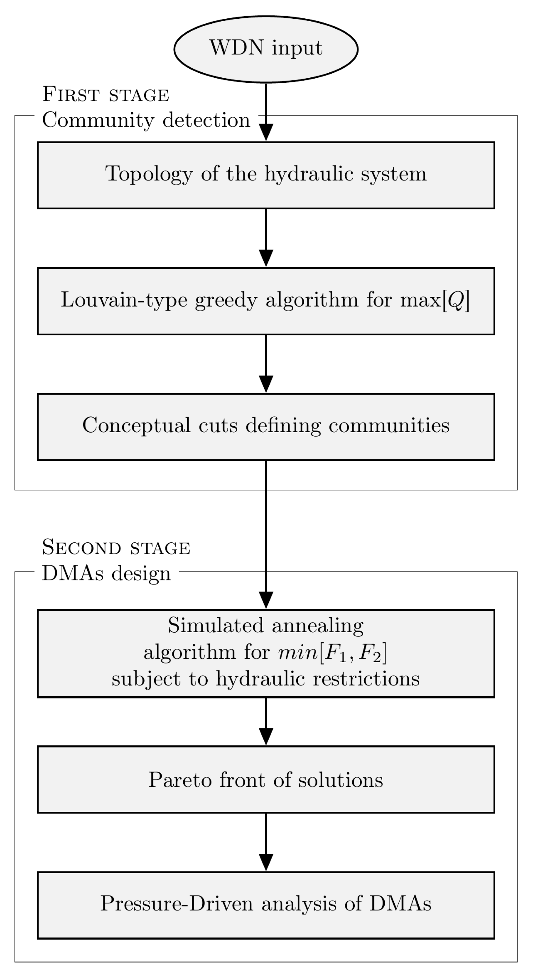
A summary of the methodology proposed in the study is shown in the flowchart of Figure 2.

2.4. Case Studies

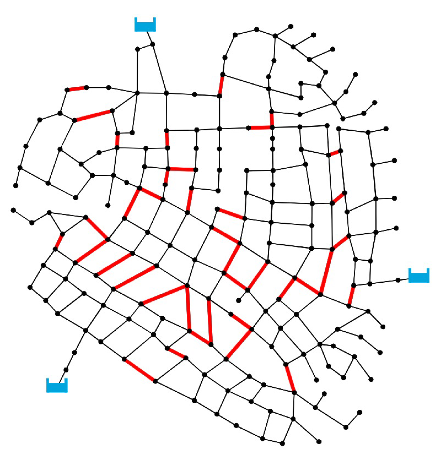
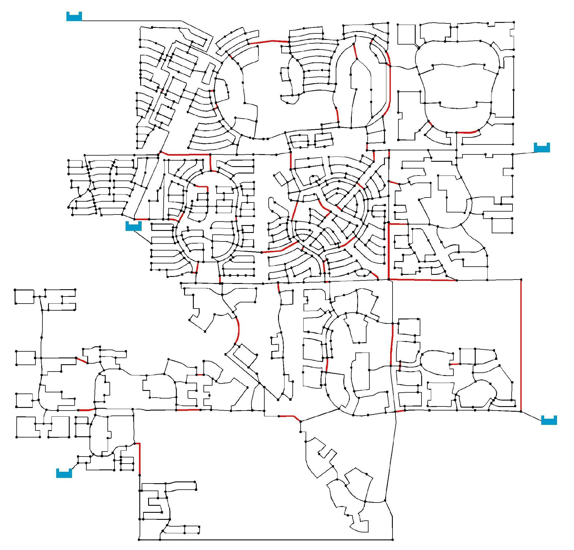
The proposed methodology was applied to two case studies. The first is the three-reservoir network (TRN) which was studied by Zheng [39]. This network is composed of 287 pipes and 202 nodes (see Figure 3). During the operation cycle, three reservoirs are used as sources. The difference between the maximum and minimum ground elevation is 37 m. Flowmeters, isolation valves or pumps are not installed in this hydraulic system. The second case is the modified large network (MLN) which was investigated by Kang and Lansey [40]. This network is composed of 5 reservoirs, 1278 pipes, 935 demand nodes, and 4 demand patterns of 24 h each (Figure 4). Here TRN is used for snapshot hydraulic simulation, while MLN is used for Extended Period Simulation (EPS).

3. Results

3.1. Case Study 1: Three-Reservoir Water Network (TRN)

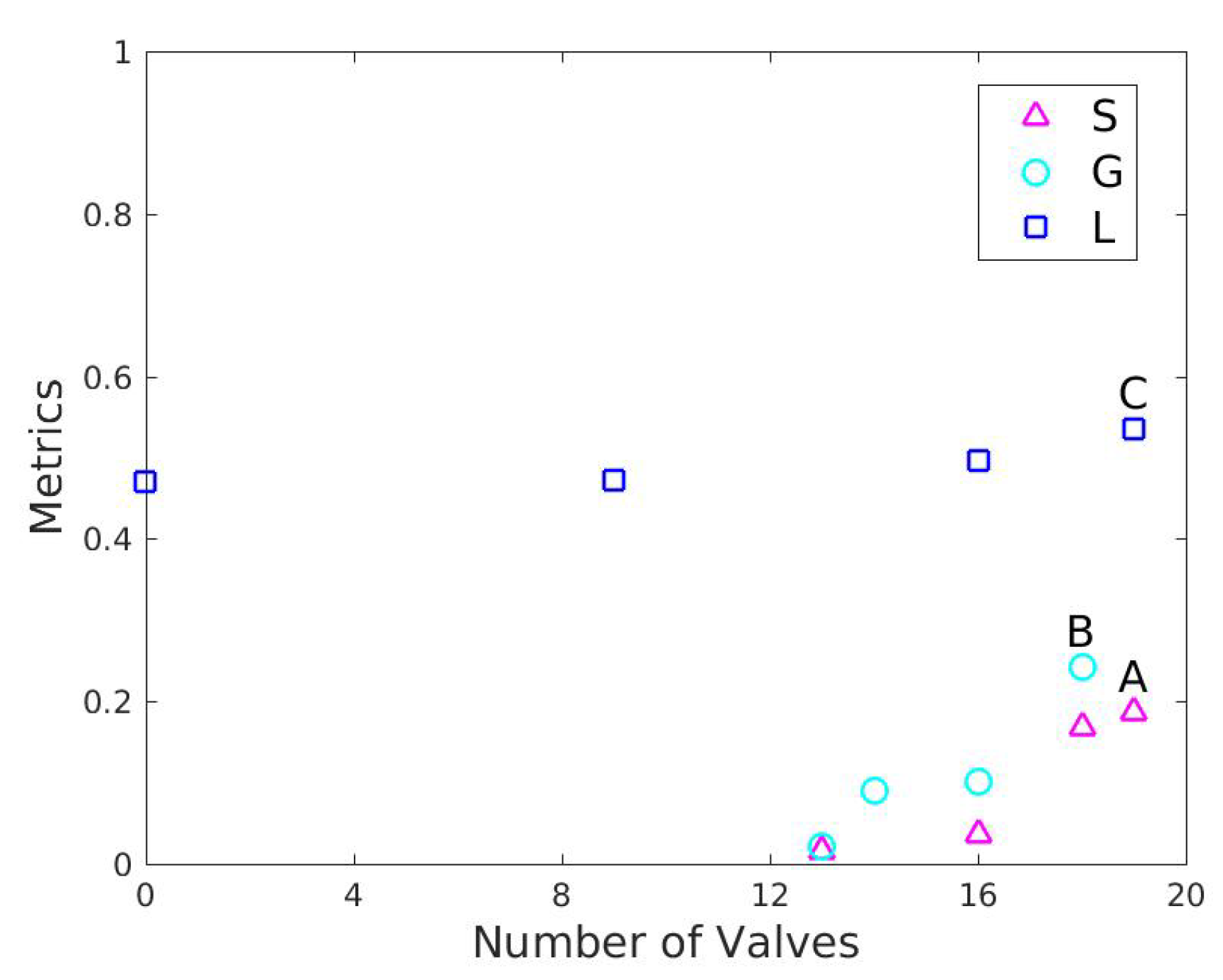
The solution with 10 communities, reported in Figure 3, corresponds to the (near) global maximum of generalized modularity obtained of a result of the first stage for the TRN network. This solution determines 38 conceptual cuts (indicated in red) and is the basis for the second phase. The second stage returned multiple DMA designs for each PI. Pareto fronts in Figure 5 show different PI values in terms of the number of valves to be installed. The main results are shown in

Table 1. Operating conditions of each solution obtained with Standard deviation for TRN network. The gray background corresponds to the solution A represented in Figure 6.

DMAs	N° Valves	L	G	S	${\mathit{P}}_{\mathit{MIN}}\left(\mathit{m}\right)$	Node Index	${\mathit{P}}_{\mathit{MAX}}\left(\mathit{m}\right)$	Node Index
3	19	0.597	0.249	0.187	4.7	161	32.4	199
3	18	0.514	0.208	0.168	9.3	118	32.6	173
2	16	0.510	0.026	0.037	9.3	118	31.8	173
3	13	0.547	0.021	0.016	7.4	136	28.4	173

,

Table 2. Operating conditions of each solution obtained with Gini coefficient for TRN network. The gray background corresponds to the solution B represented in Figure 6.

DMAs	N° Valves	L	G	S	${\mathit{P}}_{\mathit{MIN}}\left(\mathit{m}\right)$	Node Index	${\mathit{P}}_{\mathit{MAX}}\left(\mathit{m}\right)$	Node Index
3	18	0.555	0.242	0.182	7.6	118	32.5	199
3	16	0.499	0.100	0.075	12.0	5	28.9	199
2	14	0.496	0.090	0.128	13.5	5	28.9	173
3	13	0.548	0.022	0.016	7.4	136	28.4	173

and

Table 3. Operating conditions of each solution obtained with Loss of resilience for TRN network. The gray background corresponds to the solution C represented in Figure 6.

DMAs	N° Valves	L	G	S	${\mathit{P}}_{\mathit{MIN}}\left(\mathit{m}\right)$	Node Index	${\mathit{P}}_{\mathit{MAX}}\left(\mathit{m}\right)$	Node Index
3	19	0.535	0.221	0.177	6.2	118	32.9	173
3	16	0.496	0.139	0.104	12.0	5	30.0	199
2	9	0.471	0.241	0.340	15.2	136	29.8	173
0	0	0.470	-	-	15.1	118	29.7	173

where it is summarized the comparisons among all solutions in terms of the number of DMAs, the number of interventions, the value of each PI and other performance indicators of the hydraulic system, namely, extreme pressures and the node indexes where they are located. The maximum number of DMAs that is given for each PI is equal to the number of reservoirs, although each district presents special features. It should be noted that extreme pressures tend to occur on the same nodes for different objective. The only exception is the first solution shown in Table 1 where the minimum pressure occurs in a different node. In order to illustrate a particular sectorization, the gray color rows correspond to those solutions defining three DMAs with a similar number of interventions. These districts are shown in Figure 6 and correspond to solutions of the Pareto fronts with the highest number of interventions (indicated as A, B and C in Figure 5). Figure 7 graphically depicts the corresponding demand distributions for each district. The configuration obtained with standard deviation is very similar to that obtained from the Gini coefficient. Both solutions define an identical district, shaded in orange.

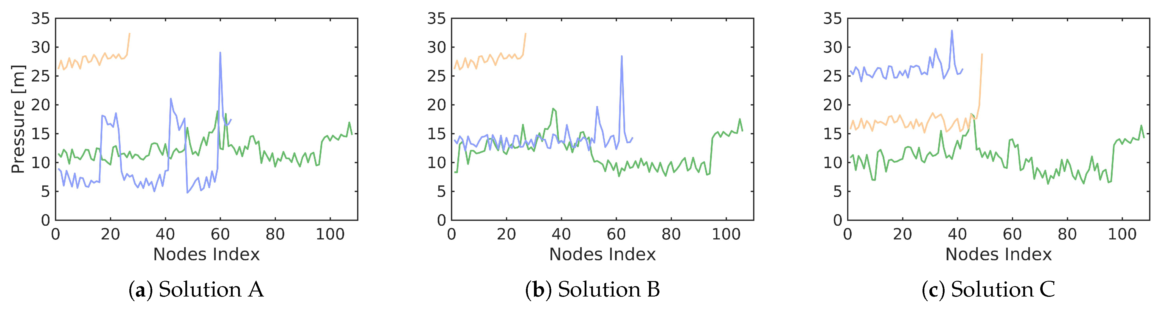
Figure 8 shows the pressures obtained for solutions A, B and C, in the extreme case in which valves are closed, isolating all the DMAs. Solution A shows the largest pressure variation across a district, for the extreme case (district shaded in light blue) the pressure varies from 5 m to 30 m of water column, which indicates that the standard deviation does not offer a good performance to achieve a homogeneous operation of the hydraulic system. Gini coefficient (solution B) generates the DMAs with the highest minimum pressures and, additionally, a more homogeneous pressures distribution between two districts (green and blue). Solution C shows a better variation of the pressures within each district, and thus, its configuration outperforms the standard deviation index and the Gini coefficient from the perspective of pressure uniformity in each autonomous DMA.

Comparing solutions A and B with solution C for the district in orange color of Figure 7, it is observed that demand increases from $15.3\%$ to $25.9\%$. This increment generates a drop in the pressures of the corresponding district with an average of $10.2$ m of water column (see Figure 8). A similar feature can be observed with the decreased demand for the district in blue color.

From Figure 8 should be noted that there are no nodes without water service. In addition, pressure-driven analysis allows to determine the percentage of the satisfied demand. For solution A, $13.6\%$ of nodes present pressures below $P^{req}$. However, $99.5\%$ of the required demands are satisfied. For solution B, all the pressures are highest than the required service pressure $P^{req}$ and, therefore, $100\%$ of required demand are satisfied. For solution C, only $3.5\%$ of the nodes present pressures values slightly lower than $P^{req}$, delivering $99.9\%$ of required demands.

3.2. Case Study 2: Five-Reservoir Water Network (MLN)

For this case study, an extended period simulation (EPS) must be evaluated in order to guarantee the required level of service for all hours under different demand patterns. As a result of the first stage, Figure 4 shows the conceptual cuts that decompose the network into 20 communities.

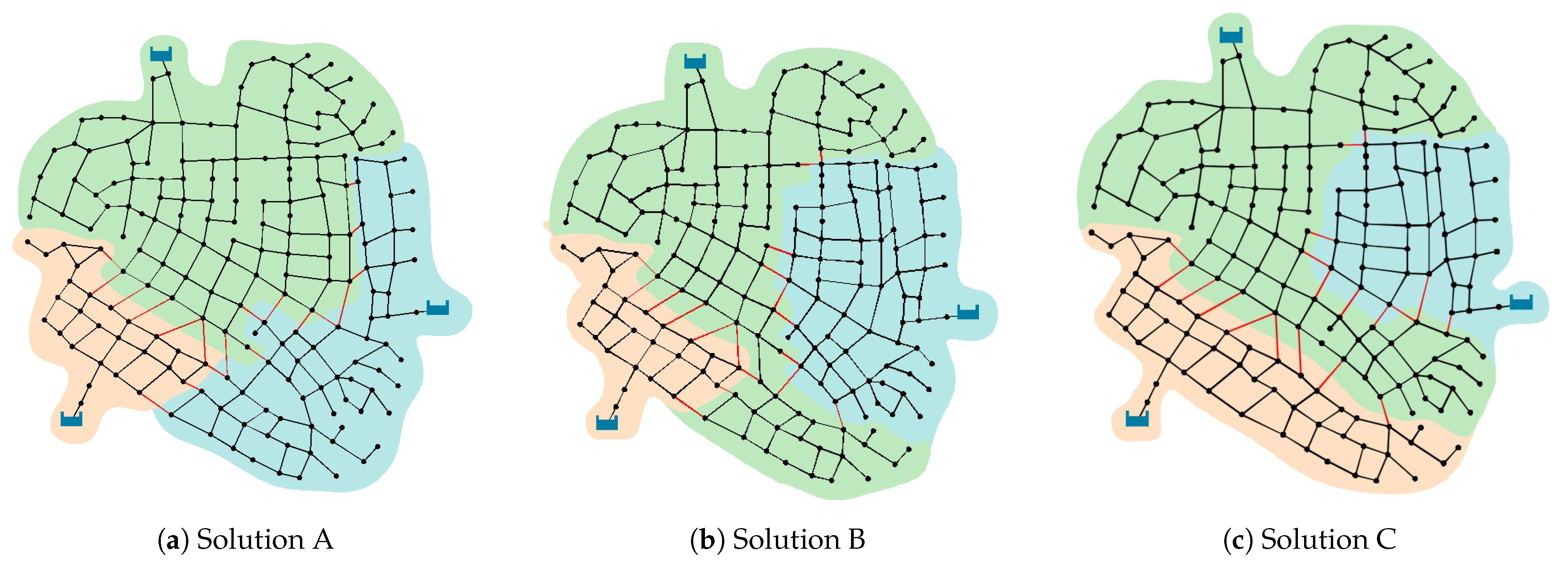
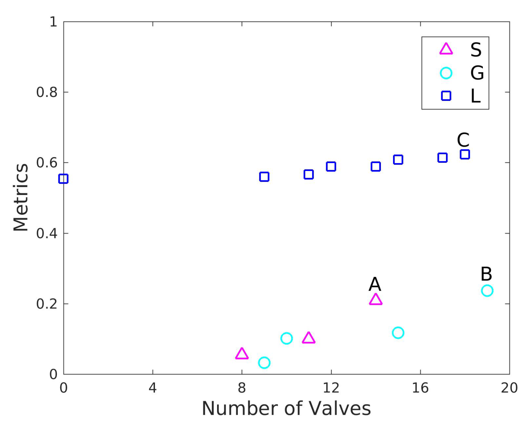
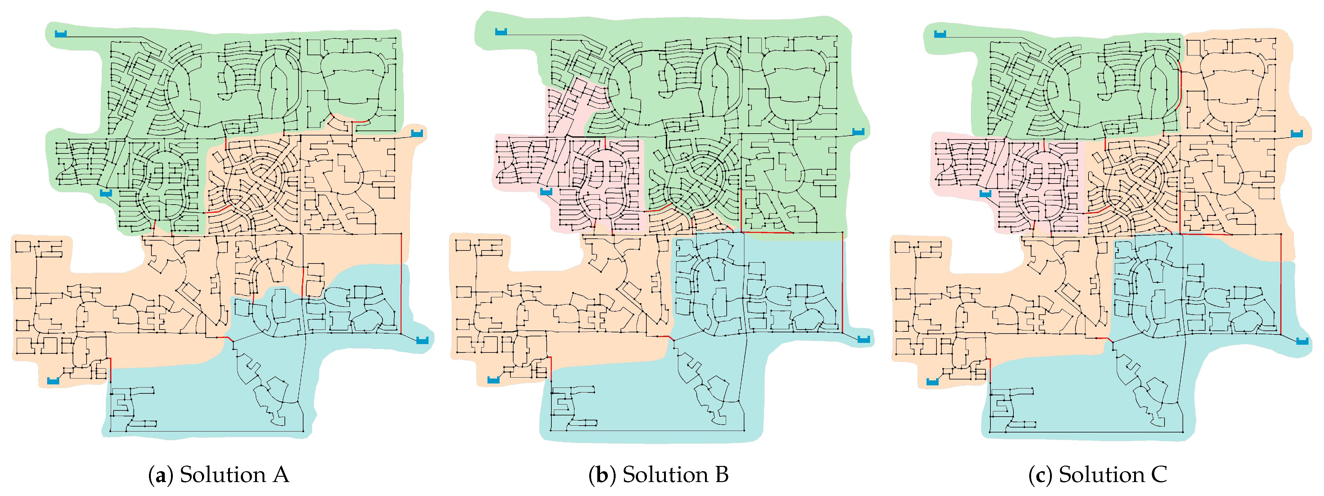
Figure 9 shows the Pareto fronts returned by the second stage optimization procedure for the different PIs of the MLN network. The performance of the hydraulic system evaluated for each solution is reported in

Table 4. Operating conditions of each solution obtained with Standard deviation for MLN network. The gray background corresponds to the solution A represented in Figure 10.

DMAs	N° Valves	L	G	S	${\mathit{P}}_{\mathit{MIN}}\left(\mathit{m}\right)$	Node Index	${\mathit{P}}_{\mathit{MAX}}\left(\mathit{m}\right)$	Node Index
3	14	0.708	0.245	0.208	4.6	846	29.5	700
2	11	0.658	0.070	0.099	5.2	303	29.0	932
2	8	0.589	0.039	0.055	5.1	627	26.6	700

,

Table 5. Operating conditions of each solution obtained with Gini coefficient for MLN network. The gray background corresponds to the solution B represented in Figure 10.

DMAs	N° Valves	L	G	S	${\mathit{P}}_{\mathit{MIN}}\left(\mathit{m}\right)$	Node Index	${\mathit{P}}_{\mathit{MAX}}\left(\mathit{m}\right)$	Node Index
4	19	0.666	0.237	0.128	4.3	362	28.7	700
3	15	0.650	0.117	0.088	4.3	362	28.4	700
2	10	0.580	0.101	0.143	7.3	289	26.3	700
2	9	0.644	0.032	0.046	4.9	535	28.0	700

and

Table 6. Operating conditions of each solution obtained with Loss of resilience for MLN network. The gray background corresponds to the solution C represented in Figure 10.

DMAs	N° Valves	L	G	S	${\mathit{P}}_{\mathit{MIN}}\left(\mathit{m}\right)$	Node Index	${\mathit{P}}_{\mathit{MAX}}\left(\mathit{m}\right)$	Node Index
4	18	0.685	0.238	0.137	4.7	535	28.7	700
4	17	0.615	0.121	0.078	6.1	159	27.7	700
3	15	0.609	0.135	0.106	6.6	502	27.7	700
3	14	0.591	0.160	0.121	6.0	159	26.8	700
2	12	0.589	0.151	0.214	6.9	159	26.8	700
3	11	0.566	0.251	0.215	6.0	159	26.2	700
2	9	0.560	0.082	0.116	9.6	159	26.2	700
0	0	0.555	-	-	10.9	303	26.2	700

. Gini coefficient and loss of resilience provide maximum number of DMAs and similar number of valves (see Table 5 and Table 6). Minimum and maximum pressures values are found between $4.3$ m and $28.7$ m. The solution for standard deviation with maximum number of interventions gives 14 valves and 3 DMAs, and pressure values into the range of $4.6$ m and $29.5$ m (Table 4). Looking for solutions with similar number of interventions, the results show differences about the efficiency of the hydraulic systems. For instance, the solution obtained with the loss of resilience for 14 valves determines 3 DMAs and a minimum pressure of $6.0$ m. Thus, in order to illustrate the system behavior in a particular scenario, the solutions with maximum number of interventions are analyzed. These solutions correspond to the gray rows in Table 4, Table 5 and Table 6 and, respectively, to solutions A, B and C of Figure 9. At first glance it seems that this comparison is biased in favor of solution A since it has a smaller number of districts than solutions B and C. However, it should be noted that a comparison of A with the solutions of the other two PIs involving the same number of districts further favors these last two metrics. The DMAs obtained for the PIs under study are shown in Figure 10. As in the first network studied, colors represent different DMAs.

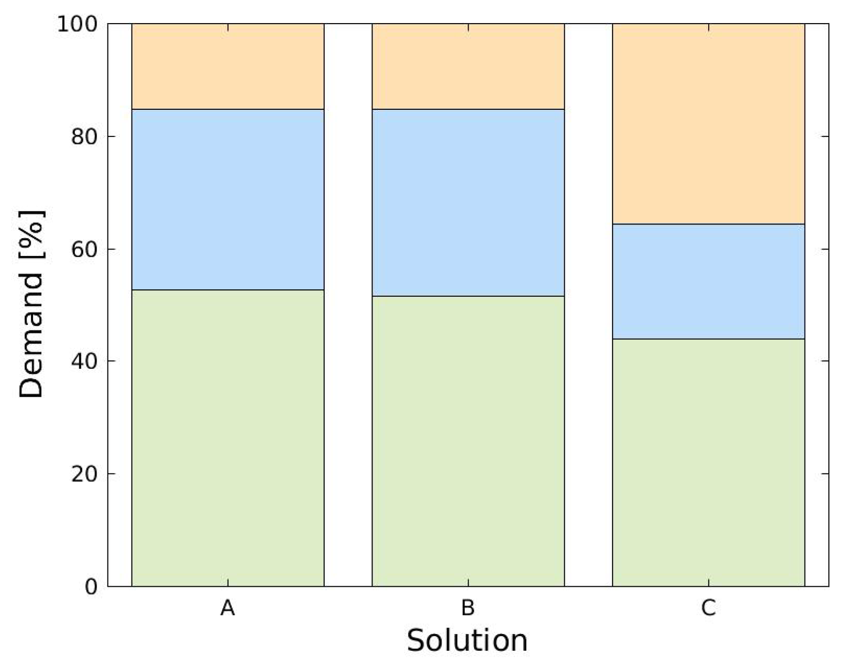
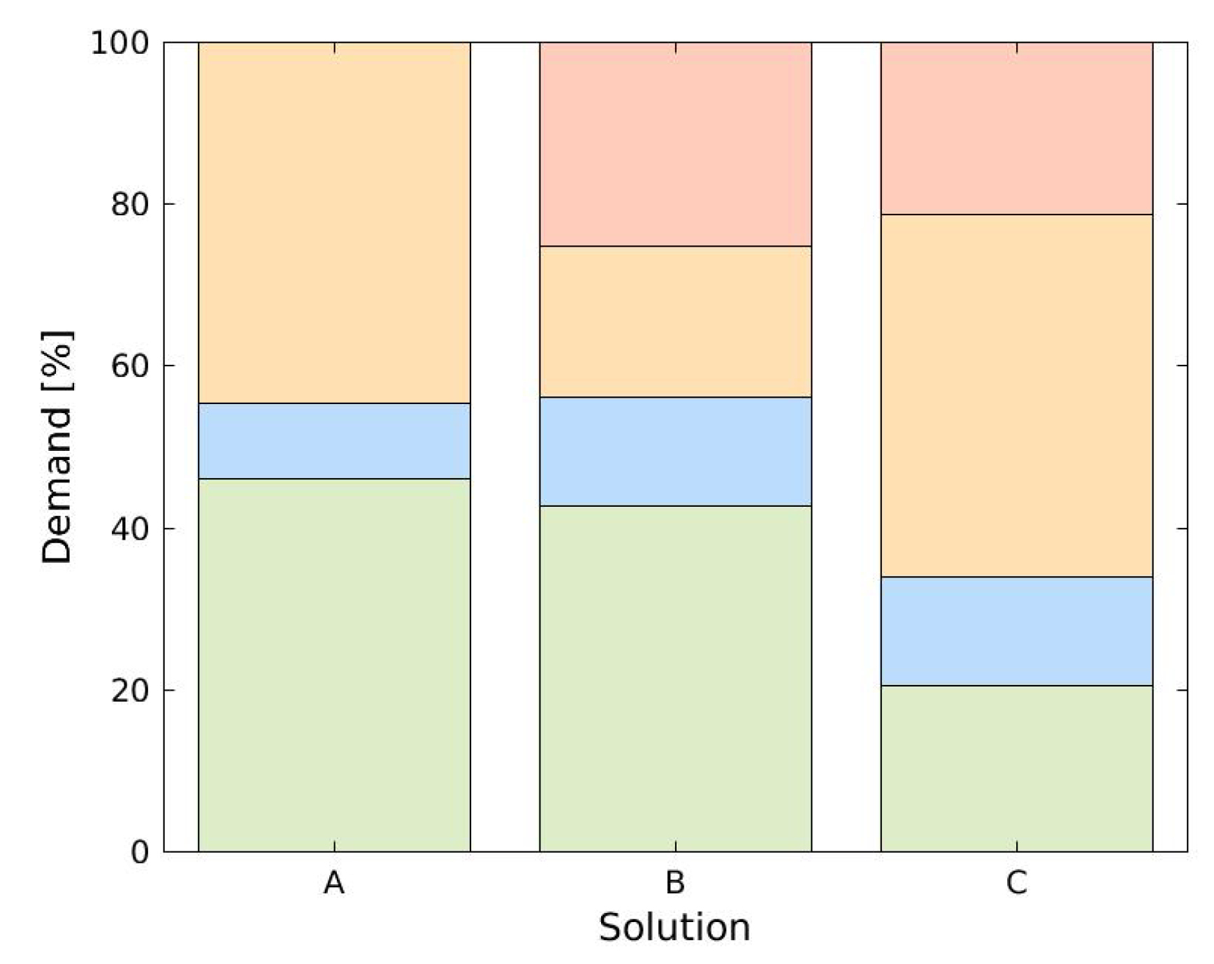
Figure 11 shows the distribution of demands for each DMA. Standard deviation solution shows poor performance when seeking homogenize demands between districts. Solution A results in two largest districts with demands of $46.1\%$ and $44.6\%$ in contrast with the $9.3\%$ of the third district.

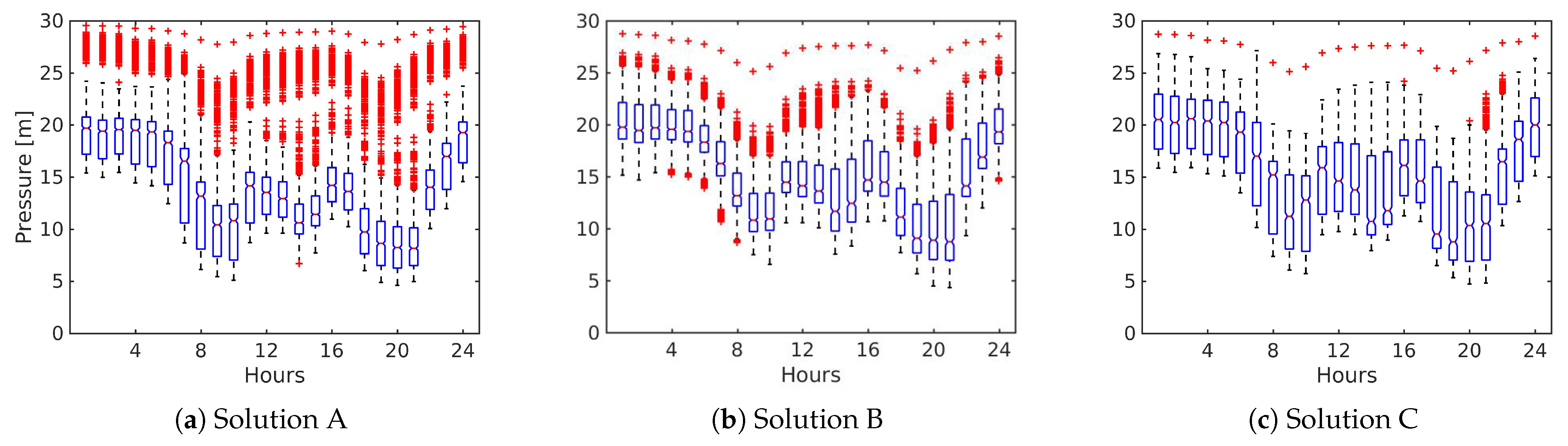
Figure 12 shows the resulting pressures for the pressure-driven analysis in the extreme case in which all the defined DMAs operate in isolation during a period of 24 h (solutions A, B and C correspond to Figure 9). Statistical maximum (top bar), statistical minimum (bottom bar), 25th and 75th percentiles (top and bottom edges of box), median (red line in box), and outliers (red crosses) are displayed. Solution A (Figure 12a) presents an asymmetry for most of the hours in the pressure boxes. It shows a large data dispersion between the 25th percentile and the median. Outliers are observed above the statistical maximum for all the hours of the analysis, likewise only for hour 14 an outlier is below the minimum. For the case of the Gini coefficient (Figure 12b), the pressures between the 25th and 75th percentile shows the least dispersion of the three solutions. Also, solution B has more outliers below the statistical minimum, but the outliers are significantly reduced above the maximum as is compared with the first solution. Solution C (Figure 12c) shows the box data with the bigger amplitude and a reduction of the outliers. In addition, this solution has the highest medians of the three best settings.

Pressure-driven analysis shows that there no nodes without water service. However, solution A presents $38\%$ of nodes with pressure values slightly below $P^{req}$ delivering $97\%$ of required demands. For solution B, $24.9\%$ of nodes present pressures below $P^{req}$ with $98.5\%$ satisfied demands. Last, for solution C, $25.9\%$ of the nodes show pressures values slightly lower than $P^{req}$, delivering $98\%$ of required demands.

4. Conclusions

This work presents a two-stage approach for the optimal design of DMAs. The general idea is to perform sectorization with the goal of identifying one source per sector. In many networks there is only one source and so the sectorization is made with the use of volume meters. In the present case the WDNs are conceived to be isolated by operating valves on the selected pipes. Determine the number and location of these pipes is proposed here as a multiobjective optimization problem. One of the typical questions is which second objective to use next to cost (or number of interventions). This question is faced and the research highlights the advantages of three criteria (objectives) when applied to real WDNs. In particular, it investigates to what extent two specific indicators, namely Gini coefficient and standard deviation, are able to provide districts with similar demands. The performance of the DMAs obtained are compared with those obtained under loss of resilience.

To achieve these goals, a methodology based on two-stage approach is developed. The first stage uses the Louvain-type greedy algorithm for the generalized modularity maximization that includes a resolution parameter for tuning the number of initial communities that are used in the second stage. Thus, the three independent two-objective optimizations of the second stage start from the same initial configuration. It is found that the application of these PIs can significantly impact differently the final configuration of the DMAs. For the cases studied, there are two different situations that restrict the number of DMAs in each network. In the first case (TRN) the maximum number of DMAs is limited by the number of existing sources. However, in the second case (MLN) the maximum number of DMAs is restricted by the hydraulic capacity of the network. That is, no more that 4 districts are able to satisfy the service conditions.

Two PIs, standard deviation and Gini coefficient, were oriented to provide districts design with similar demands. The pressure driven approach for the hydraulic analysis of the solutions indicates that Gini coefficient provided better performance than standard deviation. That is, comparing the same number of districts with similar number of valves, Gini coefficient provides solutions with lowest lost of resilience and highest minimum pressure. It should be noted that the standard deviation has a statistical bias that occurs when analyzing a low number of data and generates a lack of sensitivity of the function to achieve homogenization of the variable. That might be the reason of the low performance when compared with the other PIs. In other words, there are not enough districts for this PI to achieve a good distribution of the demands. On the other hand, when comparing the solutions provided by Gini coefficient and loss of resilience under similar conditions, the analysis indicates that loss of resilience achieves better performance for each district. Likewise, the results show that the best option when looking for pressure uniformity is to minimize the loss of resilience.

Finally, must be emphasized that engineering criteria is a key factor during the process of network partitioning that cannot be incorporated in any automatic sectorization. For instance, it must be defined the number of communities in order to start the second stage. Here it was used 10 and 20 communities, respectively, for the first and second case study. This means around 3 and 4 communities by each reservoir, but more complex networks could require a different criteria. Another example is given by the hydraulic parameters that the DMAs must satisfy. Here it was investigated two PIs for demand similarity and compared with minimum loss of resilience. However, the benefits of using different indicators should be thoroughly investigated in follow up research. Last, it is expected in the future to extend the analysis to larger WDNs and includes the leakage detection, although the two cases presented are in locations where the non revenue water is rather low.

References

- Bui, X.K.; Marlim, M.S.; Kang, D. Water Network Partitioning into District Metered Areas: A State-Of-The-Art Review. Water 2020, 12, 1002. [Google Scholar]
- Hajebi, S.; Roshani, E.; Cardozo, N.; Barrett, S.; Clarke, A.; Clarke, S. Water distribution network sectorisation using graph theory and many-objective optimisation. J. Hydroinform. 2015, 18, 77–95. [Google Scholar] [CrossRef] [Green Version]
- Chatzivasili, S.; Papadimitriou, K.; Kanakoudis, V. Optimizing the Formation of DMAs in a Water Distribution Network through Advanced Modelling. Water 2019, 11, 278. [Google Scholar] [CrossRef] [Green Version]
- DiNardo, A.; DiNatale, M. A heuristic design methodology based on graph theory for district metering of water supply networks. Procedia Eng. 2011, 43, 193–211. [Google Scholar]
- Di-Nardo, A.; Di-Natale, M.; Santonastaso, G.F.; Venticinque, S. An automated tool for smart water network partitioning. Water Resour. Manag. 2013, 27, 4493–4508. [Google Scholar] [CrossRef]
- DiNardo, A.; DiNatale, M.; Santonastaso, G.; Tzatchkov, V.; Yamanaka, V. Divide and conquer partitioning technoques for smart water netwoks. Procedia Eng. 2014, 89, 1176–1183. [Google Scholar] [CrossRef] [Green Version]
- Alvisi, S.; Franchini, M. A heuristic procedure for the automatic creation of district metered areas in water distribution systems. Urban Water J. 2014, 11, 137–159. [Google Scholar] [CrossRef]
- Scarpa, F.; Lobba, A.; Becciu, G. Elementary DMA Design of Looped Water Distribution Networks with Multiple Sources. J. Water Resour. Plan. Manag. 2016, 142, 04016011. [Google Scholar] [CrossRef] [Green Version]
- Zevnik, J.; Kramar-Fijavž, M.; Kozelj, D. Generalized Normalized Cut and Spanning Trees for Water Distribution Network Partitioning. J. Water Resour. Plan. Manag. 2019, 145, 04019041. [Google Scholar] [CrossRef]
- Zhang, K.; Yan, H.; Zeng, H.; Xin, K.; Tao, T. A practical multi-objective optimization sectorization method for water distribution network. Sci. Total. Environ. 2019, 656, 1401–1412. [Google Scholar] [CrossRef]
- Scibetta, M.; Boano, F.; Revelli, R.; Ridolfi, L. Community detection as a tool for district metered areas identification. Procedia Eng. 2014, 70, 1518–1523. [Google Scholar] [CrossRef] [Green Version]
- Giustolisi, O.; Ridolfi, L. New Modularity-Based Approach to Segmentation of Water Distribution Networks. J. Hydraul. 2014, 140, 1–14. [Google Scholar] [CrossRef]
- Campbell, E.; Ayala-Cabrera, D.; Izquierdo, J.; Perez-García, R.; Tavera, M. Warer supply network sectorizarion based on social networks community detection algorithms. Procedia Eng. 2014, 89, 1208–1215. [Google Scholar] [CrossRef] [Green Version]
- Giustolisi, O.; Ridolfi, L.; Berardi, L. General metrics for segmenting infrastructure networks. J. Hydroinform. 2015, 17, 505–517. [Google Scholar] [CrossRef]
- Castro-Gama, M.; Pan, Q.; Jonoski, A.; Solomatine, D. A graph theorical sectorization approach for energy reduction in water distribution networks. Procedia Eng. 2016, 154, 19–26. [Google Scholar] [CrossRef] [Green Version]
- Laucelli, D.B.; Simone, A.; Berardi, L.; Giustolisi, O. Optimal Design of District Metering Areas. Procedia Eng. 2016, 162, 403–410. [Google Scholar] [CrossRef] [Green Version]
- Zhang, Q.; Wu, Z.Y.; Zhao, M.; Qi, J. Automatic partitioning of water distribution networks using multiscale community detection and multiobjective optimization. J. Water Resour. Plan. Manag. 2017, 149, 04017057. [Google Scholar] [CrossRef]
- Di-Nardo, A.; Di-Natale, M.; Di-Mauro, A.; Martinez-Díaz, E.; Blazquez-García, J.; Santonastaso, G.; Tuccinardi, F. An advanced software to design automatically permanent partitioning of a water distribution network. Urban Water J. 2020, 17, 259–265. [Google Scholar] [CrossRef]
- Herrera, M.; Izquierdo, J.; Perez-García, R.; Ayala-Cabrera, D. Water Supply Clusters by Multi-Agent Based Approach. In Proceedings of the Water Distribution System Analysis 2010–WDSA2010, Tucson, AZ, USA, 12–15 September 2010; pp. 861–869. [Google Scholar]
- Liu, H.; Zhao, M.; Zhang, C.; Fu, G. Comparing Topological Partitioning Methods for District Metered Areas in the Water Distribution Network. Water 2018, 10, 368. [Google Scholar] [CrossRef] [Green Version]
- Perelman, L.S.; Allen, M.; Preis, A.; Iqbal, M.; Whittle, A.J. Automated sub-zoning of water distribution systems. Environ. Model. Softw. 2015, 65, 1–14. [Google Scholar] [CrossRef] [Green Version]
- Di-Nardo, A.; Di-Natale, M.; Santonastaso, G.F.; Venticinque, S. Graph partitioning for automatic sectorization of a water distribution system. In Proceedings of the Computer and Control in Water Industry CCWI, Exeter, UK, 5–7 September 2011; pp. 841–846. [Google Scholar]
- Vasilic, Z.; Stanic, M.; Kapelan, Z.; Prodanovic, D.; Babic, B. Uniformity and Heuristics-Based DeNSE Method for Sectorization of Water Distribution Networks. J. Water Resour. Plan. Manag. 2020, 146, 04019079. [Google Scholar] [CrossRef] [Green Version]
- Shao, Y.; Yao, H.; Zhang, T.; Chu, S.; Liu, X. An Improved Genetic Algorithm for Optimal Layout of Flow Meters and Valves in Water Network Partitioning. Water 2019, 11, 1087. [Google Scholar] [CrossRef] [Green Version]
- Creaco, E.; Cunha, M.; Franchini, M. Using heuristic techniques to account for engineering aspects in modularity-based water distribution network partitioning algorithm. J. Water Resour. Plan. Manag. 2019, 145, 04019062. [Google Scholar] [CrossRef]
- Giudicianni, C.; Herrera, M.; Di-Nardo, A.; Carravetta, A.; Ramos, H.M.; Adeyeye, K. Zero-net energy management for the monitoring and control of dynamically-partitioned smart water systems. J. Clean. Prod. 2020, 252, 119745. [Google Scholar] [CrossRef]
- Giudicianni, C.; Herrera, M.; Di-Nardo, A.; Adeyeye, K. Automatic multiscale approach for water networks partitioning into dynamic district metered areas. Water Resour. Manag. 2020, 34, 835–848. [Google Scholar] [CrossRef] [Green Version]
- Rahmani, F.; Muhammed, K.; Behzadian, K.; Farmani, R. Optimal Operation of Water Distribution Systems Using a Graph Theory-Based Configuration of District Metered Areas. J. Water Resour. Plan. Manag. 2018, 144, 04018042. [Google Scholar] [CrossRef]
- Saldarriaga, J.; Bohorquez, J.; Celeita, D.; Vega, L.; Paez, D.; Savic, D.; Dandy, G.; Filion, Y.; Grayman, W.; Kapelan, Z. Battle of the Water Networks District Metered Areas. J. Water Resour. Plan. Manag. 2019, 145, 04019002. [Google Scholar] [CrossRef]
- Newman, M.E.J.; Girvan, M. Finding and evaluating community structure in networks. Phys. Rev. E 2004, 69, 026113. [Google Scholar] [CrossRef] [Green Version]
- Newman, M.E.J. Modularity and community structure in netwoks. Proc. Natl. Acad. Sci. USA 2006, 103, 8577–8582. [Google Scholar] [CrossRef] [Green Version]
- Blondel, V.D.; Guillaume, J.; Lambiotte, R.; Lefebvre, E. Fast unfolding of communities in large networks. J. Stat. Mech. Theor. Exper. 2008, 10, P10008. [Google Scholar] [CrossRef] [Green Version]
- Jeub, L.; Bazziand, M.; Jutla, I.; Mucha, P. A Generalized Louvain Method for Community Detection Implemented in MATLAB. 2011–2019. Available online: https://github.com/GenLouvain/GenLouvain (accessed on 18 November 2019).
- Reichardt, J.; Bornholdt, S. Detecting Fuzzy Community Structures in Complex Networks with a Potts Model. Phys. Rev. Lett. 2004, 93, 218701. [Google Scholar] [CrossRef] [PubMed] [Green Version]
- Gomes, R.; Marques, A.; Sousa, J. identification of the optimal entry points at District Metered Areas and implementation of pressure management. Urban Water J. 2012, 9, 365–384. [Google Scholar] [CrossRef]
- Castro-Gama, M.; Pan, Q.; Jonoski, A.; Chiesa, C. Model-Based Sectorization of Water Distribution Networks For Increased Energy Efficiency. In Proceedings of the HIC2014, New York, NY, USA, 17–21 August 2014. Paper 233. [Google Scholar]
- Castro-Gama, M.; Popescu, I.; Jonoski, A.; Pan, Q. Towards increased water and energy efficiencies in water distribution systems. Environ. Eng. Manag. J. 2015, 14, 1271–1278. [Google Scholar]
- Castro-Gama, M.; Lanfranchi, E.; Pan, Q.; Jonoski, A. Water distribution network model building, case study: Milano, Italy. Procedia Eng. 2015, 119, 573–582. [Google Scholar]
- Zheng, F.; Zecchin, A. An efficient decomposition and dual-stage multi-objective optimization method for water distribution systems with multiple supply sources. Environ. Model. Softw. 2014, 55, 143–155. [Google Scholar] [CrossRef]
- Kang, D.; Lansey, K. Revisiting Optimal Water-Distribution System Design: Issues and a Heuristic Hierarchical Approach. J. Water Resour. Plan. Manag. 2012, 138, 208–217. [Google Scholar] [CrossRef]
- Alireza, Y.; Paul, J. Complex network analysis of water distribution systems. Chaos Interdiscip. J. Nonlinear Sci. 2011, 21, 016111. [Google Scholar] [CrossRef] [Green Version]
- Todini, E.; Pilati, S. A gradient algorithm for the analysis of pipe networks. In Computer Application in Water Supply, System Analysis and Simulation; John Wiley: London, UK, 1988; Volume I, pp. 1–20. [Google Scholar]
- Porter, M.A.; Onnela, J.; Mucha, P.J. Communities in Networks. Not. AMS 2009, 56, 1082–1097. [Google Scholar]
- Fortunato, S. Community detection in graphs. Phys. Rep. 2010, 486, 75–174. [Google Scholar] [CrossRef] [Green Version]
- Brandes, U.; Delling, D.; Gaertler, M.; Gorke, R.; Hoefer, M.; Nikoloski, Z.; Wagner, D. On finding graph clusterings with maximum modularity. In Graph-Theoretic Concepts in Computer Science, WG 2007. Lecture Notes in Computer Science; Springer: Berlin, Germany, 2007; Volume 4769, pp. 121–132. [Google Scholar]
- Todini, E. Looped water distribution netowrks design using a resilience index based heuristic approach. Urban Water 2000, 2, 115–122. [Google Scholar] [CrossRef]
- Giustolisi, O.; Savic, D.; Kapelan, Z. Pressure-Driven Demand and Leakage Simulation for Water Distribution Networks. J. Hydraul. Eng. 2008, 134, 626–635. [Google Scholar] [CrossRef] [Green Version]
- Wagner, J.; Shamir, U.; Marks, D. Water distributions system reliability: Simulation methods. J. Water Resour. Plan. Manag. 1988, 114, 276–294. [Google Scholar] [CrossRef] [Green Version]
- Kirkpatrick, S.; Gelatt, C.; Vecchi, M. Optimization by simulated annealing. Science 1983, 220, 671–680. [Google Scholar] [CrossRef] [PubMed]
- Schneider, J.J.; Kirkpatrick, S. Stochastic Optimization; Springer Science & Business Media: Berlin/Heidelberg, Germany, 2006. [Google Scholar]
- Suman, B.; Kumar, P. A survey of simulated annealing as a tool for single and multiobjective optimization. J. Oper. Res. Soc. 2006, 57, 1143–1160. [Google Scholar] [CrossRef]
- Suppapitnarm, A.; Seffen, K.; Parks, G.; Clarkson, P. Simulated annealing: An alternative approach to true multiobjective optimization. Eng. Optim. 2000, 33, 59–85. [Google Scholar] [CrossRef]
Figure 1.
Schematic process of district metering areas (DMAs) design for a simple network.
Figure 2.
Conceptual flowchart of the procedure.
Figure 3.
Conceptual cuts obtained for the three-reservoir network (TRN).
Figure 4.
Conceptual cuts obtained for the modified large network (MLN).
Figure 5.
Pareto front of solutions for the three-reservoir network (TRN) obtained with the three studied performance indices (PIs). Legend: S: Standard deviation, G: Gini coefficient, L: Loss of resilience.
Figure 6.
DMAs obtained after the second stage for each PI. (a) Standard deviation, (b) Gini coefficient and (c) Loss of resilience. Solutions correspond to those indicated in Figure 5 and to the gray color rows in Tables.
Figure 7.
Demand distribution per DMA for solution A, B and C for TRN network. Colors code corresponding to DMAs of Figure 6.
Figure 8.
Nodal pressures for the solutions A, B and C for TRN network. Colors code corresponding to DMAs of Figure 6 and Figure 7.
Figure 9.
Pareto front of solutions for MLN network obtained with the three studied PIs. Legend: S: Standard deviation, G: Gini coefficient, L: Loss of resilience.
Figure 10.
DMAs obtained for MLN network. Solutions A, B and C are those indicated in Figure 9 for (a) Standard deviation, (b) Gini coefficient and (c) Loss of resilience.
Figure 11.
Demand distribution per DMAs for solutions A, B and C for MLN network. Code colors corresponding to DMAs of Figure 10.
Figure 12.
Temporal variation of pressure for solution A, B and C for MLN network. Each time step represents a box plot for the pressure of all nodes of the network.