Article

A Comparative Assessment of Hydrological Models in the Upper Cauvery Catchment

1
UK Centre for Ecology & Hydrology, Wallingford OX10 8BB, UK
2
Department of Civil Engineering, Indian Institute of Science, Bangalore 560012, India
3
Divecha Centre for Climate Change, Indian Institute of Science, Bangalore 560012, India
4
International Crops Research Institute for the Semi-Arid Tropics, Hyderabad 502324, India
5
Interdisciplinary Centre for Water Research, Indian Institute of Science, Bangalore 560012, India
*
Author to whom correspondence should be addressed.
Water 2021, 13(2), 151; https://doi.org/10.3390/w13020151
Submission received: 2 December 2020 / Revised: 24 December 2020 / Accepted: 4 January 2021 / Published: 11 January 2021
(This article belongs to the Special Issue Modelling Hydrologic Response of Non­-homogeneous Catchments)

Abstract

:
This paper presents a comparison of the predictive capability of three hydrological models, and a mean ensemble of these models, in a heavily influenced catchment in Peninsular India: GWAVA (Global Water AVailability Assessment) model, SWAT (Soil Water Assessment Tool) and VIC (Variable Infiltration Capacity) model. The performance of the three models and their ensemble were investigated in five sub-catchments in the upstream reaches of the Cauvery river catchment. Model performances for monthly streamflow simulations from 1983–2005 were analysed using Nash-Sutcliffe efficiency, Kling-Gupta efficiency and percent bias. The predictive capability for each model was compared, and the ability to accurately represent key catchment hydrological processes is discussed. This highlighted the importance of an accurate spatial representation of precipitation for input into hydrological models, and that comprehensive reservoir functionality is paramount to obtaining good results in this region. The performance of the mean ensemble was analysed to determine whether the application of a multi-model ensemble approach can be useful in overcoming the uncertainties associated with individual models. It was demonstrated that the ensemble mean has a better predictive ability in catchments with reservoirs than the individual models, with Nash-Sutcliffe values between 0.49 and 0.92. Therefore, utilising multiple models could be a suitable methodology to offset uncertainty in input data and poor reservoir operation functionality within individual models.

1. Introduction

Hydrological models are widely used for the prediction and understanding of hydrological processes [1,2]. Models are powerful tools to understand and quantify the components of the water balance and hydrological fluxes within a catchment [3] by designing simplified conceptual representations of the complex hydrological cycle using various parameters and sets of mathematical equations [4,5,6]. The performance [7] and suitability [8] of a hydrological model can differ between catchments due to catchment size and dominant catchment processes present. Hydrological models are often developed for specific purposes (estimation of water demands, understanding of hydrological processes, drought and flood risk assessments, etc.) and for different geographic regions [9]. The most reliable models in regions where data is sparse, are ones whose results closely represent reality with the use of limited model complexity [10]. It is important to note that the selection of a suitable model should not be solely based on its ability to address specific research aims but also data availability [11]. The accuracy of simulations generated from the model is strongly dependent on the model selected and the quality of input data and observations [11]. For example, in instances of poor quality input data with high uncertainties, a simpler model may be more suitable than a highly complex one [12].
Various hydrological models have different strengths when representing hydrological processes [13]. The use of a single model can lead to simulation uncertainties especially in catchments of poor input data availability and in large-scale modelling exercises. Ensemble modelling combines multiple model predictions to create a single prediction that tends to strongly outperform the individual models [14,15]. Ensemble modelling can be widely applied in hydrological modelling to utilise the ensemble for reducing errors with an optimal bias [16]. It is also important to note that a combination of the best performing individual models do not necessarily provide the best ensemble [17].
The Cauvery has long presented water management challenges at the local, regional and catchment scales. The increasing competition to meet urban and rural water demands, which span administrative boundaries, continue to present significant issues for integrated water management in the catchment. Key gaps remain in the scientific knowledge of Peninsular Indian hydrology that make it difficult to address these concerns.
Many of the sub-catchments of the Cauvery catchment have been previously modelled using the SWAT (Soil Water Assessment Tool) model [18,19], the Water Evaluation And Planning System (WEAP) model [20], remote sensing methods [21], Artificial Neural Network (ANN) and Support Vector Regression (SVR) models [22], the Soil Conservation Service Curve Number (SCS-CN) model [23,24] and Variable Infiltration Capacity-Macroscale Hydrologic Model (VIC-mHM) [25]. Understanding the river flows in headwater catchments is especially relevant for estimating actual water availability across the catchment. The Western Ghats form the headwaters of the Upper Cauvery catchments. This region generates the majority of the streamflow with the greater Cauvery catchment. Representing the catchments using multiple models can provide deeper insight into hydrological processes across the region and analysing a model ensemble can reduce uncertainty within the estimation of various components of the water balance. This study attempts to analyse the capability of the above-mentioned models and a model ensemble to capture processes in a catchment.
For this study, five sub-catchments within the Upper Cauvery region were selected to be modelled by SWAT, VIC and GWAVA. The GWAVA (Global Water AVailability Assessment) model is a gridded large-scale water resources model developed by the UK Centre for Ecology & Hydrology [26]. It is a relatively simple model that trades off model complexity for data availability, plus has a strong anthropogenic influences component. VIC (Variable Infiltration Capacity) model has a much more detailed representation of hydrological components and is perhaps more suitable for an accurate representation of soil water dynamics. SWAT is commonly used in India and has a good representation of agricultural water use with possibly better representation of evaporation.
VIC model has been widely utilised and performs well for a large number of river catchments across the globe. The model is open-source and has wide acceptance and utility because of its proven capability in capturing streamflow processes as well as all the components of the water budget. The model uses complex, widely accepted algorithms for the simulation of hydrological processes such as evaporation, transpiration and infiltration which has been validated over many river catchments of the Indian subcontinent. The model was selected for application in the Cauvery Catchment, as it is a grid-based model which takes into account the sub-grid variability of the land surface vegetation classes and soil moisture storage capacity. GWAVA is a useful tool in the Cauvery Catchment as it allows for the simulation of most of the components of the hydrological cycle as well as accounting for demands for domestic, agricultural and industrial sectors, reservoir operation and the inclusion of interventions. The model allows for the tracking of groundwater, reservoir storage levels and the demands that are not able to be met. The model input and output are flexible to the data availability and the output requirements. As Cauvery is a highly heterogenous catchment concerning the climate, soil composition and land use, it is important to incorporate these gridded models to capture the extensive regional variability within the catchment.
SWAT has been widely used across India and around the globe. The model is popular due to the ability to use the model through an ArcGIS interface and the model can be set with minimum data and facilitate the user to set the model as per the availability of their data in terms of LULC, soil, biophysical and its management information. SWAT does not need grid specific information. In addition, and of high importance within the Cauvery, small agricultural management interventions can be parameterised, reservoir operations can be included, groundwater usage can be set, and crop management operation can be defined.
Ensemble modelling is a process where multiple models are utilised to simulate an outcome by using many different modelling algorithms. The mean ensemble model averages the prediction of each model and produces one final simulation of the outcome. Ensemble modelling can be utilised in hydrology to better simulate components of the hydrological cycle, the impacts of land use or other environmental changes, provide a range of possible outcomes and uncertainty [27,28,29]. In larger catchments with relatively poor input data availability, the use of a single model can lead to simulation uncertainties. Ensemble modelling combines multiple model predictions to create a single prediction that tends to strongly outperform the individual models [14,15]. Ensemble modelling can be widely applied to utilise the ensemble for reducing errors with an optimal bias [16].
This study investigates the predictive capabilities of GWAVA, SWAT, and VIC when applied to several sub-catchments in the Cauvery, and the performance of a mean ensemble of these models. Model performance is assessed using a range of efficiency metrics (Nash-Sutcliffe efficiency, Kling-Gupta efficiency and percent bias). The comparative strengths and weaknesses of each model are assessed by analysing model performance in the difference sub-catchments, this gives insight into the suitability of these models for future studies under similar conditions. The mean ensemble is analysed to determine whether an ensemble approach can successfully combine model strengths and compensate for model limitations.

2. Model Descriptions

It is of importance to evaluate how different hydrological models capture the process dynamics of various catchments. In this study, three hydrological models were used to model the Upper Cauvery catchment: Variable Infiltration Capacity model (VIC), Soil Water Assessment Tool (SWAT) and Global Water AVailability Assessment model (GWAVA). SWAT [30] GWAVA [31] and VIC [25,32] have been applied across large regions of India. The models were selected based on the various theoretical differences and previous applications in India. VIC and SWAT are popular hydrological models across India and GWAVA has been successfully implemented in the Narmada and Ganges catchments. VIC is a large-scale, physically-based gridded hydrological model, GWAVA is a large-scale semi-distributed hydrological model whilst SWAT is a semi-distributed, physically-based catchment-scale model. VIC, SWAT and GWAVA are described below and additional information can be found in Appendix A in Table A1. Each model was calibrated using different techniques however the calibration parameters utilised in each case pertained to soil properties and surface-and groundwater routing.

2.1. Variable Infiltration Capacity (VIC) Model

The VIC model [33,34] is an open-source, grid-based macroscale land-atmosphere transfer model that represents surface and subsurface hydrological processes. It solves the energy and water balance equations at each time step for spatially distributed grid cells. The model can be implemented for spatial scales varying from 0.125 to 2 degrees and with temporal resolutions ranging from hourly to daily. The key features of the model include the representation of sub-grid vegetation heterogeneity, non-linear baseflow computation and inclusion of multiple soil layers with variable infiltration. Each grid cell can be divided into several tiles based on the land use and each tile generates unique responses to precipitation based on the land surface properties. The VIC model has been extensively implemented for numerous studies across the globe to address challenges related to water resources management such as flood and drought monitoring [35,36,37], assessment of the impact of land use and climate change on the hydrologic response [25,32] and understanding land-atmosphere interactions [38,39,40]. Meteorological forcings required to run the model include precipitation, maximum temperature, minimum temperature and wind speed at the relevant time-scale. This model also requires additional datasets such as elevation, soil characteristics which consist of soil composition and bulk density, along with vegetation properties such as land-use type, leaf-area index (LAI), albedo and crop characteristics. For simulating streamflow at the specified gauge locations, the flux files are fed into a routing model [41], which uses linear transfer functions for grid cells as well as river routing and linearised Saint-Venant equation for channel routing. This version of VIC does not account for any water demands, groundwater pumping or reservoir storage. The output fluxes from the model are surface runoff, baseflow, evapotranspiration and soil moisture computed for each grid.

2.2. Soil and Water Assessment Tool (SWAT)

SWAT is an open-source software widely used around the globe to assess the impact of sediment transport, fertiliser load and different water management practices in an agricultural catchment [42]. ArcSWAT, a version of SWAT interfaced with ArcGIS, can be used for continuous simulation of a catchment model operating on different time steps and at different spatial scales. In SWAT, a catchment is divided into multiple sub-catchments, which are further divided as Hydrological Response Units (HRUs). HRUs are unique combinations of a specific soil type, land use/land cover type and slope type within a sub-catchment for which the water balance components can be simulated. It is important to note that HRUs vary in size and as a general rule should have between one and ten HRUs per sub-catchment. SWAT is capable of predicting hourly, daily, monthly and yearly flow volumes. Climatic inputs include daily precipitation, maximum and minimum temperature, solar radiation, relative humidity and wind speed. Various hydrologic processes can be simulated using the SWAT model, including surface runoff, lateral subsurface flow, groundwater flow, evapotranspiration, snowmelt, transmission losses from streams, and water storage and losses from ponds [43].

2.3. Global Water Availability Assessment (GWAVA) Model

GWAVA is a large-scale gridded water resources model [26,44]. The model accounts for natural hydrological processes (taking into account soils, land use and lakes) and anthropogenic influences (crops, domestic and industrial demands, reservoir operations, and water transfers). The model estimates surface flows and recharge using a conceptual rainfall-runoff model, utilising effective precipitation and evaporation estimates, followed by a demand-driven routine to account for the anthropogenic stresses on the system. The model can be run at a spatial-scale ranging from 0.125 to 5 degree and either at a daily or monthly time-scale. The GWAVA model is adaptable to the data availability of the region and the code is flexible to allow for additional processes and features to be represented. GWAVA has been updated recently to better represent both groundwater abstraction and artificial recharge based largely of the principles of the AMBHAS-1D model [45]. Whereby the groundwater store is recharged from the soil moisture, lakes and reservoirs, leaking infrastructure and small-scale storage interventions. A further recent update to GWAVA has been to incorporate a representation of check dams, farm bunds and urban tanks into the model structure [46].

3. Model Applications and Comparison

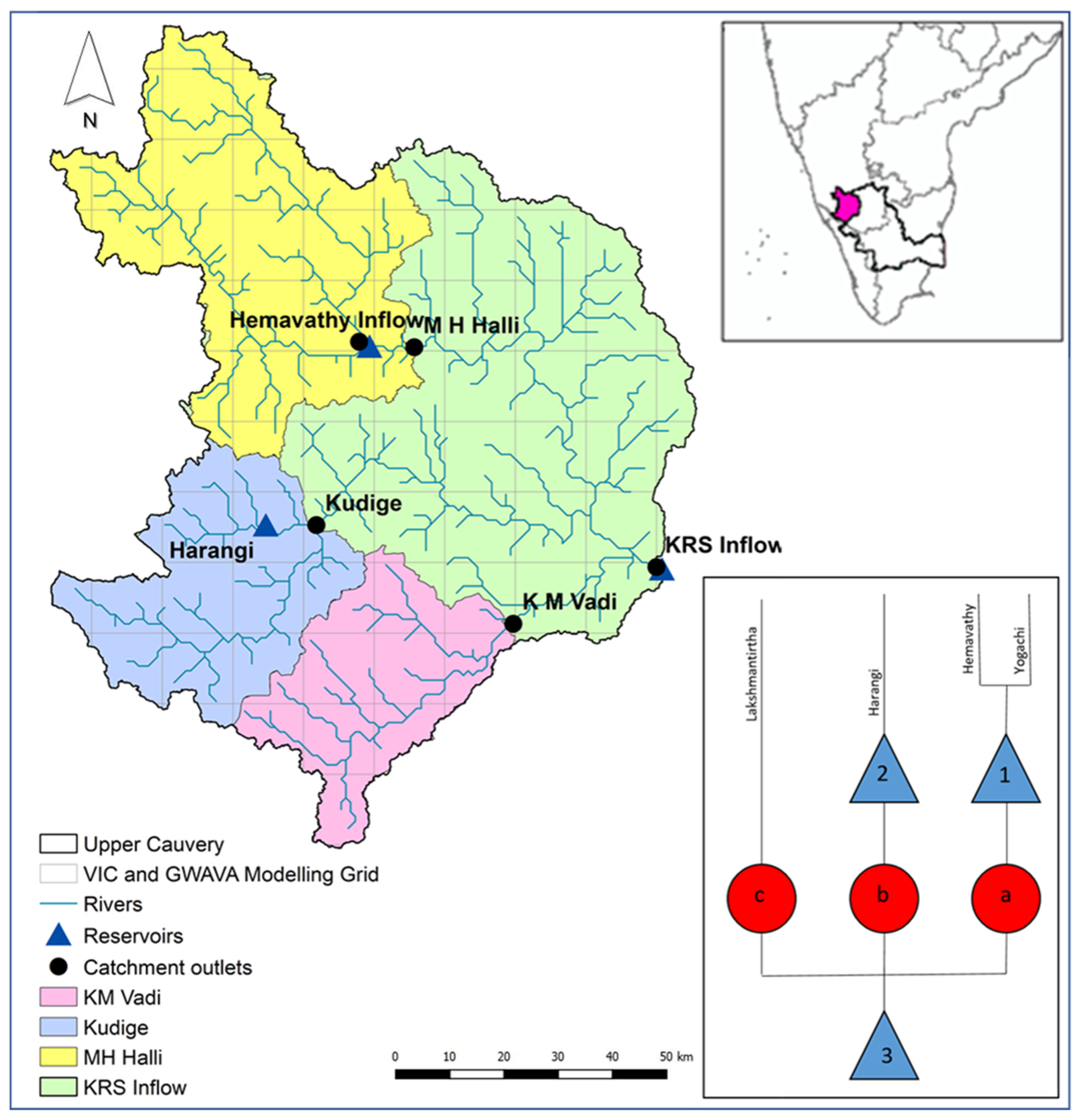
3.1. Site Description

The Cauvery catchment is a heterogeneous, transboundary and highly human-influenced catchment, in Peninsular India. It is spread across four federal states, namely, Karnataka, Tamil Nadu, Kerala and Puducherry in Southern India [18]. The four states have varying water policy, water use prioritisation and cultural value associated with the natural environment. The catchment is a representative of other large catchments in Peninsular India, with water resources under increasing pressure from urbanisation, population growth and agriculture intensification. Additionally, the Cauvery is a contentious river with concern over the sharing of water between Karnataka and Tamil Nadu. The catchment is considered to be highly water-stressed [47] and the current water abstraction is estimated to exceed the renewable water resources within the catchment [48]. The catchment has extensive regional variability in water demand. The agricultural activities within the catchment require approximately 90% of water resources [49,50]. Rapid urban and industrial development across the catchment are causing increased inter-sectorial and interstate competition for water [51]. Across the catchment, there is an abundance of small-scale storage interventions, medium and large reservoirs, and large-scale transfer schemes. It is essential to have a good understanding of the catchment hydrology and develop reliable and robust models to ensure improved water resource management in such highly water-stressed catchments.
The Upper Cauvery catchment drains an area 10,619 km2 in the north-western region of the Cauvery catchment. The upper reaches of the Cauvery River lie within the Nilgiri and Anaimalai mountains and act as a critical headwater to the larger catchment [52]. The sub-catchment experiences both the SW (JJAS) and NE monsoon (OND). The mean annual rainfall in the Upper Cauvery is 2010 mm however; the rainfall distribution varies temporally and spatially across the sub-catchment. The Western Ghats form a rain-shadow along the western coastline, decreasing the precipitation gradient during the south-western monsoon [53]. The mean daily temperatures vary between 9 °C and 25 °C throughout the catchment [54]. In the area of the Western Ghats, the soils tend to be very deep, valley bottoms covered in dense forests and mountain slopes are predominately grassland [55]. Fifty percent of the sub-catchment is under agriculture [56]. The most common crops grown in the catchment are sugarcane, finger millet, sorghum, groundnut and paddy. Paddy and sugarcane are found predominantly in the canal command areas.
Five catchments were chosen for the study, namely the catchments upstream of (Figure 1): Kudige on the Harangi River; K M Vadi on the Lakshmantirtha River; M H Halli, immediately downstream of the Hemavathy Reservoir; the inflow of the Hemavathy Reservoir (here forward referred to as Hemavathy); and the inflow to KRS reservoir (here forward referred to as KRS). More information regarding these catchments can be found in Table 1. Both Hemavathy inflow and M H Halli were chosen to assess the models’ ability to simulate the outflow releases from Hemavathy. All five were modelled by VIC and GWAVA on a daily timestep (and aggregated to monthly) and by SWAT on a monthly timestep, as monthly timesteps are generally considered most useful for impact assessments. Kudige, K M Vadi and M H Halli are locations of existing streamflow gauges whilst Hemavathy and KRS are reservoirs with observed inflows and outflows. These catchments were selected based on their importance within the Cauvery catchment and observation data availability. The performance of the individual models as well as the model ensemble was evaluated against the observation data.

3.2. Input Data and Model Application

All three models utilised precipitation and temperature forcing data [57] along with data regarding the soil, land-use and altitude. Additionally, the models made use of many local datasets which can be found in Appendix A in Table A2. The performance of the individual models as well as the model ensemble was evaluated against the observed streamflow data provided by WRIS-India. Hereafter the term virgin simulations refer to simulations that do not include any forcing with the observed reservoir outflow data.

3.2.1. VIC

VIC-3L (VIC-3 layer); version 4.2.d [58] with the Lohmann routing model [41] was run in the water balance mode. The water balance model does not solve the surface energy balance [59]. This mode assumes that the land surface soil temperature equals the near-surface air temperature and it follows the continuity equation at each time step. A daily time step was adopted for computational efficiency based on data availability. Daily simulations were aggregated to monthly estimates for this study. Two versions of the VIC model were set up for Cauvery catchment (Figure 1) at 0.125° grids and the surface fluxes were computed at daily time scale for the years 1951–2014. The first model V-VIC did not incorporate any artificial influences or reservoirs. The second F-VIC utilised the observed reservoir release data to account for two of the major reservoirs within the catchment by addition the observation data to the V-VIC simulation streamflow (Harangi and Hemavathy). The V-VIC model was calibrated with respect to observed streamflow at four stations within the region using model parameters as suggested by Lohmann et al. (1998). The runoff hydrograph was found to be governed by three parameters related to the vegetation and soil properties. The overland flow was sensitive to the variable infiltration curve parameter (B) whilst the baseflow had significant sensitivity concerning the fraction of maximum velocity of baseflow where nonlinear baseflow begins (Ds) and the fraction of maximum soil moisture where nonlinear baseflow occurs (Ws) [32,34]. Thus, these three parameters were chosen for calibration and all the other soil and vegetation parameters were obtained from the soil [60] and land use land cover datasets (Table A2, Appendix A). To account for the reservoir operation in VIC, the daily simulated streamflow was aggregated to a monthly flow and the monthly observed reservoir outflow releases were added to obtain the F-VIC simulations.

3.2.2. SWAT

This study utilised SWAT2012 [61] on ArcGIS 10.5 platform. The catchment and its sub-catchments (129 in numbers) were delineated based on the Digital Elevation Model (DEM) and defining the inflow to KRS reservoir as the catchment outlet. Land use map, soil map and slope (sources described in Table A1, Appendix A) maps were used in the creation of 4432 HRUs based on defining the threshold of 20% for each land use, soil and slope. As far as possible, the soil parameters were either measured or surveyed [62], failing which they were estimated based on literature. Further, the daily meteorological data of rainfall, temperature, wind speed, relative humidity and sunshine hours (sources described in Table A1, Appendix A) were given as input to the model. Penman-Monteith method was adopted in this study for the estimation of potential evaporation. The Curve Number (CN) method was selected for the calculation of surface runoff as it was deemed the most suitable for rainfall data at a daily time step.
The intervention density (in-situ and ex-situ) within these catchments was estimated based on expenditure reports for the Karnataka Watershed Authority. As the expenditure spent on each type of intervention was not known, the average cost for constructing each intervention based on earlier experience was used and then the total cost estimated was converted in terms of storages capacities. Conceptually, the interventions were considered to only exist within areas of agriculture (7272 km2; 70% of the total area). The most common agricultural and water management interventions were considered including check dam and bunds to represent in-situ and ex-situ intervention, respectively. The aggregated district-level catchment interventions storages were all lumped together into a single unit reservoir along the main channel of sub-catchment. Total storage capacity created due to interventions over the catchment was estimated to be 5 m3/ha in 2006. The depth of the check dam and infiltration rate observed during the survey was 1.5 m and 10 cm/day and that of bunds as 0.3 m and 30 cm/day, respectively [62]. Along with the intervention storages, the three major reservoirs (Harangi, Hemvathy and KRS) were incorporated at each sub-catchment as per their actual locations. For these major reservoirs, along with storage capacities and their surface areas, the monthly outflows were also provided as inputs to the model. There is the option in SWAT to bypass the simulation of reservoir outflow and providing the observed outflow time-series. These gauging points were fed the monthly reservoir outflow data from Hemavathy and Harangi reservoirs. This allowed the model to potentially better represent the streamflow at the gauges downstream of the reservoirs. Further, the SWAT model was calibrated for the KRS inflows from 1981 through 2003 using parameters that are related to surface runoff and baseflow. A list of these parameters can be found in Appendix A, Table A3.

3.2.3. GWAVA

Surface water flows across the Cauvery catchment (to Musiri) on a daily timestep were estimated utilizing GWAVA 5.0 [46,63]. Similarly, to VIC, GWAVA was set up for the extent of the Cauvery catchment upstream of Musiri (Figure 1) at 0.125° grids for the years 1986–2005. A grid cell resolution of 0.125° was chosen based on data availability for the region. The model setup is described in detail in Horan et al. (2020) [46] and Keller et al. (in prep). The model was calibrated, to daily observed streamflow, and validated, to daily observed streamflow and seasonal groundwater levels at 14 gauging stations across the catchment from 1980–2005 depending on the period of uninterrupted reliable observed streamflow available from the gauging station. The model included the improved groundwater module [46] demands (domestic, industrial, agricultural, livestock and the associated conveyance losses and return flows), interventions-tanks, check dams and farm bunds [46]. Five parameters were selected in the calibration. These parameters pertain to soil characteristics, surface and groundwater routing and water table level at which baseflow flows. The characteristics of the check dams and field bunds used in the GWAVA modelling exercise were the same as for the SWAT set up described in Section 3.2 and an additional description of the implementation of interventions into GWAVA can be found in Horan et al. (2020) [46].

3.3. Model Performance Criteria

The performance measures used in this study are the Nash–Sutcliffe efficiency (NSE), Kling-Gupta efficiency (KGE) and percent bias (Bias). NSE is a popular metric to evaluate hydrological model performance because it aims to normalise model performance into an interpretable scale [64,65]. An NSE of one represents a perfect correspondence between the simulations and the observations. An NSE of zero indicates that the model simulations have the same explanatory power as the mean of the observations. An NSE of less than 0 represents that the model is a worse predictor than the mean of the observations. However, NSE does not provide an equal benchmark for different flow regimes. Utilising the single NSE metric is not sufficient for determining the performance of a model, however, can provide context if utilised in conjunction with additional model performance efficiencies. For the purpose of this study, an NSE score of less than 0.2 is deemed poor, between 0.2 and 0.6 as fair and above 0.6 as good. The NSE is calculated as:
NSE = 1 t = 1 T ( Q s t Q o t ) 2 t = 1 T ( Q o t Q o ¯ ) 2
where Q s t and Q o t are, respectively, the simulated streamflow, and the observed streamflow at timestep t; Q o ¯ is the average observed streamflow over all timestep considered.
The KGE is based on correlation, variability bias and mean bias [64,66]. The metric allows some perceived shortcomings with NSE to be overcome and has become increasingly popular for the evaluation of hydrological model skill. A KGE of one indicates perfect agreement between simulations and observations. However, there are many opinions as to where the differentiation of a ‘good’ and ‘poor’ model performance thresholds lies within the KGE scale. Negative KGE values do not always imply that the model performs worse than the mean flow benchmark. For the purpose of this study and to be able to compare model performance, a KGE score of less than 0.2 is deemed poor, between 0.2 and 0.6 as fair and above 0.6 as good. The KGE is calculated as:
KGE = 1 ( r 1 ) 2 + ( σ s σ o 1 ) 2 + ( μ s μ o 1 ) 2
where r is the correlation coefficient between simulated and observed data, σ o is the standard deviation of observation data, σ s is the standard deviation of simulated data, μ o is the mean of observation data and μ s is the mean of simulated data.
The bias is the average tendency of the simulated data to over-or under-estimate the observed data. The optimal value for the bias is zero. Positive values indicate a model under-estimation and negative values indicate an over-estimation.
Bias = t = 1 T ( y o y s ) t = 1 n y o × 100
where y o is the observed data value, y s is the simulated data value and t is the time-step.
The daily streamflow volume from VIC and GWAVA was summed to generate the monthly streamflow in order for the VIC and GWAVA simulations to be comparable to the SWAT simulations, and because monthly timesteps are generally preferred for impact assessments. For the ensemble average evaluation, mean monthly streamflow was generated by averaging the monthly streamflow from F-VIC, F-SWAT and GWAVA. The model performance efficiencies were calculated from the monthly observed streamflow and the mean monthly ensemble streamflow time-series.
Monthly streamflow simulations were undertaken by VIC, GWAVA and SWAT. Virgin simulations from SWAT (V-SWAT) and VIC (V-VIC) were included in the analysis of results. The second set of simulations from SWAT (F-SWAT) and VIC (F-VIC) are improvements on the virgin simulations utilising this observed data. The calibration parameters were kept consistent between V-SWAT and F-SWAT, and V-VIC and F-VIC respectively.

4. Results

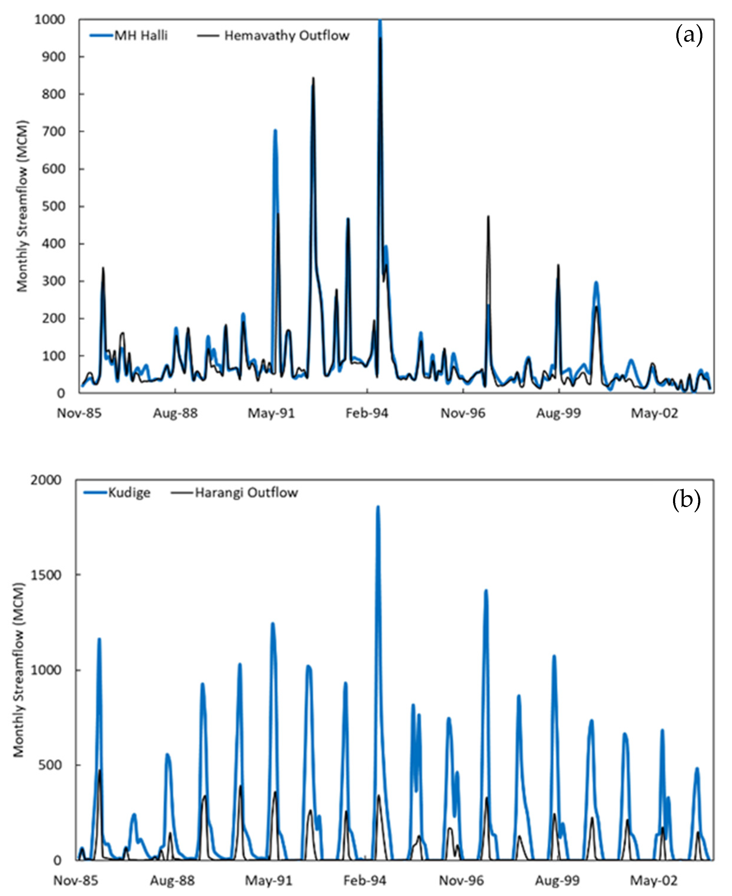
4.1. Reservoir Outflow Evaluation

To establish confidence within the observed reservoir outflow data used to force F-SWAT and F-VIC, it was compared to streamflow gauges downstream of the reservoir. Harangi reservoir outflow was compared to Kudige and Hemavathy outflow was compared with M H Halli. The gauging stations (Kudige and M H Halli) are situated a short distance downstream of the reservoirs (Harangi and Hemavathy). The Hemavathy outflow and streamflow observed at M H Halli correspond well, although the reservoir outflow does not follow a seasonal trend year on year (Figure 2a). The Harangi outflow is significantly less than the streamflow observed at Kudige (Figure 2b) this is to be expected as Kudige drains a larger area than the Harangi reservoir. However, the coinciding of the peak streamflow indicates that the temporal trend of the reservoir release is seasonal.

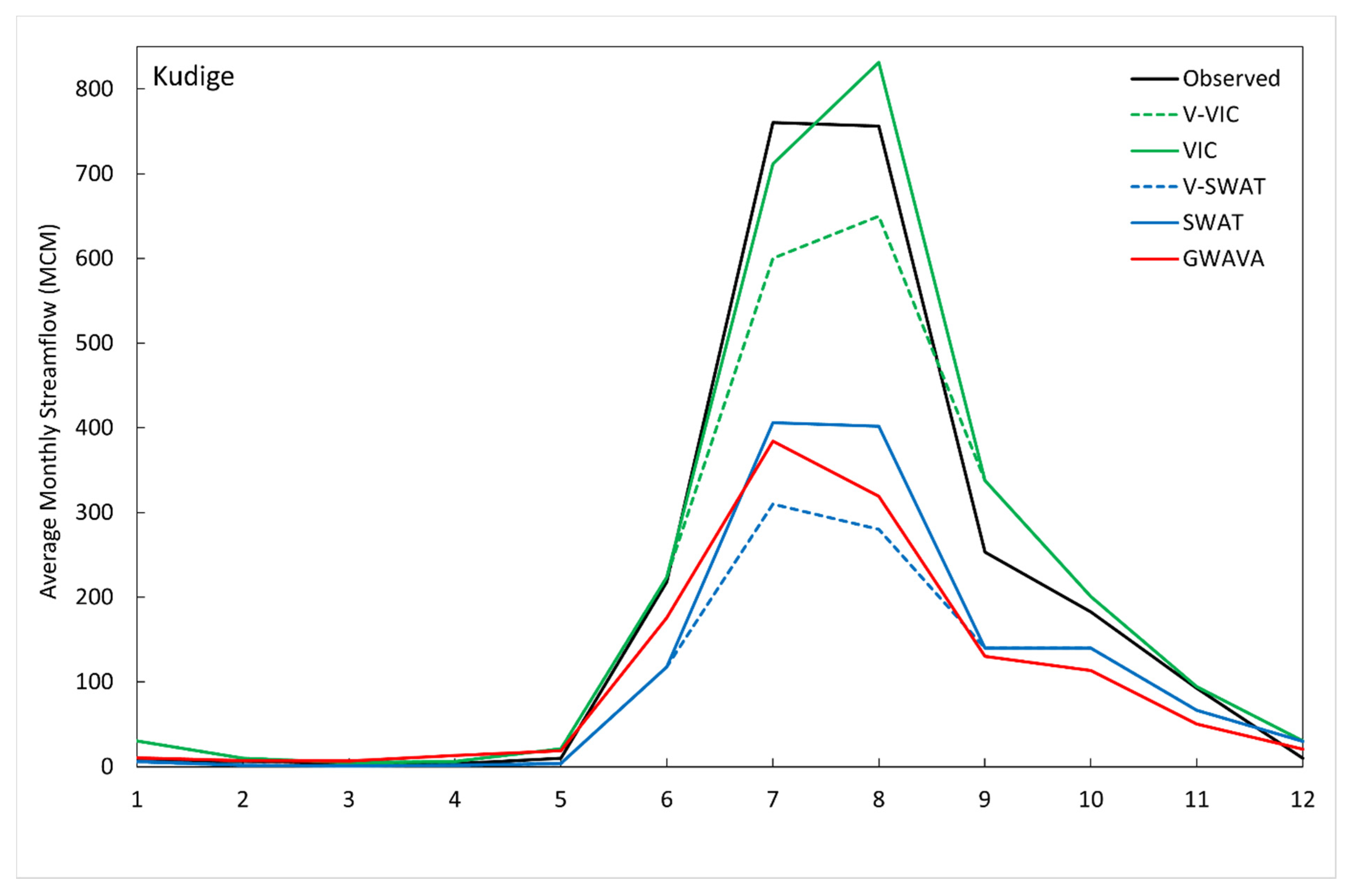
4.2. Individual Model Performance

The calibrated model performance of V-VIC, F-VIC, V-SWAT, F-SWAT and GWAVA was evaluated using the NSE, KGE and the percent bias at five gauging points in the Upper Cauvery from 1986 until 2003 (Table 2, Table 3 and Table 4) The performance of the models used in this study are compared to existing studies in Table 5.
The forcing of the streamflow with the observed reservoir data improves the simulations by F-VIC in the catchments that contain the large reservoirs (Kudige, M H Halli and KRS). However, the inclusion of this observation data causes the model to over-estimate the streamflow across these catchments. F-VIC performs well at Kudige, poorly at KRS and fairly across the remaining catchments (Table 2 and Table 3). The performance of both V-VIC and F-VIC is generally weaker in the monsoon season (Figure A1). VIC produces a low bias at Kudige but over-estimates at Hemavathy, M H Halli and K M Vadi and severely over-estimates at KRS inflow (Table 4). F-VIC simulates the monthly average streamflow well at Kudige (Figure A1). The streamflow is over-estimated in August but the rising and falling limbs are simulated well. At K M Vadi, F-VIC captures the rising limb of the hydrograph well, however, over-estimates the streamflow in August and subsequently over-estimates on the falling limb. At M H Halli, Hemavathy and KRS, F-VIC simulates the shape of the hydrograph well but significantly over-estimates the streamflow across the year (Figure A1). The over-estimation of streamflow by F-VIC downstream of the reservoirs could be a reflection of the inability of the model to account for anthropogenic water abstraction and the uncertainty in the observed reservoir outflow data and methodology used to incorporate the observed reservoir releases could contribute to poor performances at KRS.
The V-SWAT simulations under-estimate the volume of streamflow at Kudige, M H Halli and KRS and provide fair simulations at Kudige and KRS, however, the performance at M H Halli is very poor (Table 2, Table 4 and Table 5). Following the use of the observed reservoir outflow data to force the model, the performance at Kudige, M H Halli and KRS are significantly improved. When utilising the observed reservoir data, SWAT consistently performs well across the five catchments (Table 2, Table 4 and Table 5).
SWAT simulates the total streamflow volume well at K M Vadi but under-estimates in the remaining catchments (Table 4). Despite being fed the Harangi outflow data upstream, SWAT under-estimates the streamflow at Kudige. SWAT simulates the streamflow at M H Halli and K M Vadi well in July but does not retain the peak flow through August. The model simulates the second peak in October which corresponds with VIC and GWAVA but not the observed streamflow data (Figure A1). SWAT simulates the peak streamflow at Hemavathy well, however, under-estimates both the rise and falling limbs of the hydrograph. At KRS, SWAT under-estimates the peak streamflow in July and August but over-estimates the falling limb of the hydrograph.
GWAVA performs fairly across all the catchments across the modelling period (Table 2, Table 4 and Table 5) and the monsoon season. However, GWAVA performs less well at M H Halli. GWAVA under-estimates the total streamflow volume in all the catchments throughout the year (Table 4) but over-estimates the total streamflow volume at M H Halli in the monsoon season (Figure A1). The peak simulated streamflow followed the trend of the observed streamflow but is under-estimated at both Kudige and M H Halli. At K M Vadi, GWAVA significantly under-estimates the peak flows through July and August, however, peaks in October. This second peak does not correspond to the observed streamflow. At KRS, GWAVA is significantly under-estimating the streamflow throughout the year. GWAVA is inaccurately representing the outflows from Hemavathy. This is clearly illustrated by poor simulations and over-estimation of streamflow at M H Halli. The under-estimations of streamflow by GWAVA at Hemavathy, K M Vadi and downstream of Harangi could be a reflection of the inability of the model to capture the outflow characteristics of this reservoir, an over-estimation of the reservoir capacity (due to undocumented silting), misrepresentation of the interventions, the poor representation of rainfall in the IMD grids or an over-estimation of the anthropogenic and agricultural water abstraction.

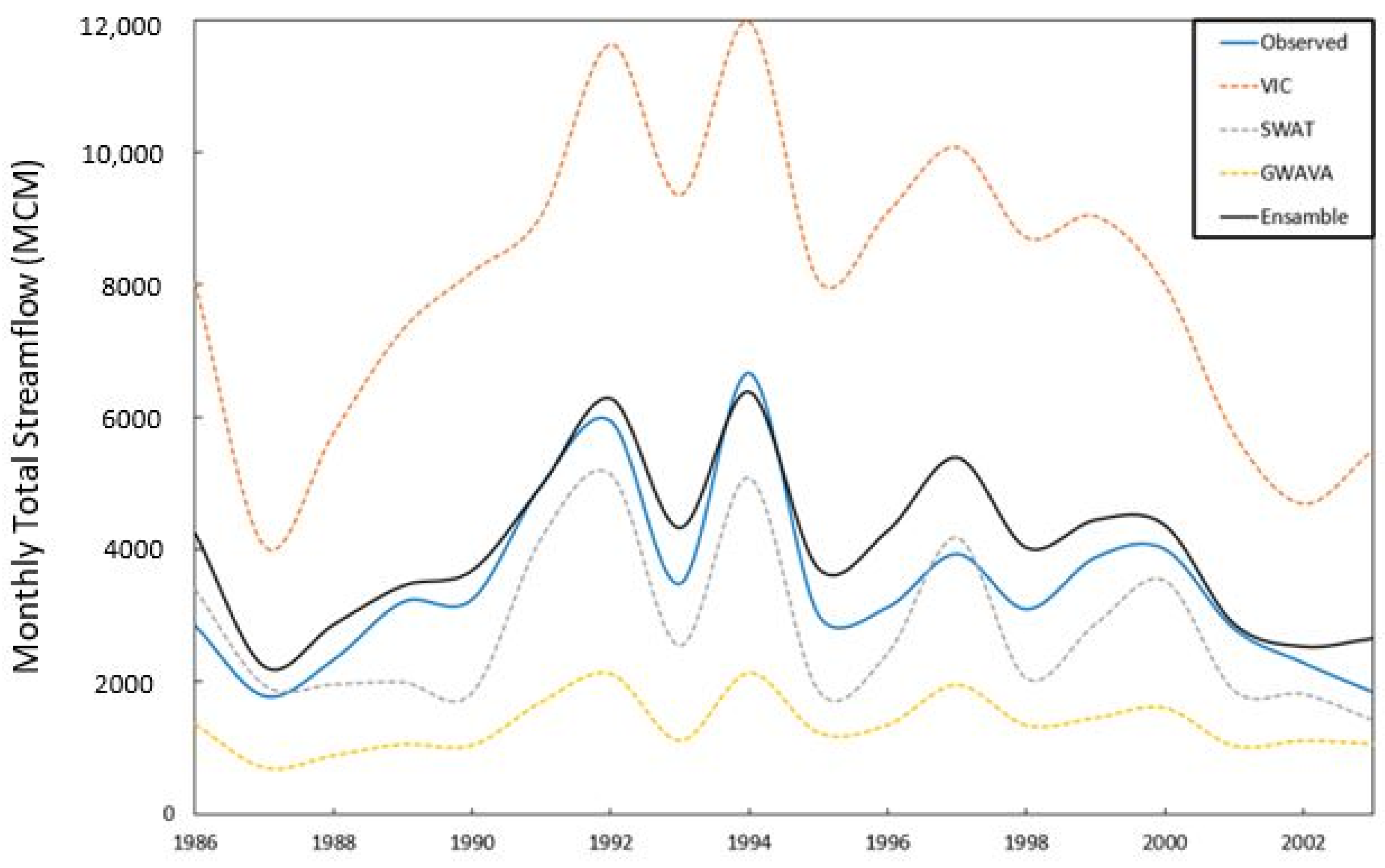
4.3. Ensemble Model Performance

The ensemble model mean was calculated using the simulations from F-VIC, F-SWAT and GWAVA. The ensemble model simulations are the most consistent with the observation streamflow. The ensemble mean of the streamflow produced by the three models proved to better represent the total volume of observed streamflow across the Upper Cauvery than the individual models (Table 4). The ensemble produced NSE values at Kudige, M H Halli, Hemavathy and KRS close to the optimal NSE of one which is a significant improvement than from the individual model NSE values (Table 2). Although the ensemble performs less well at K M Vadi, it proves to outperform the individual models (Table 2). The ensemble closely represents the observed data temporally at KRS (Figure 3). Although the ensemble generally over-estimated the volume of streamflow, and to a greater extent for the period 1995–1999, it represents the volume of streamflow more accurately than any of the individual models (Figure 3).

5. Discussion

The models individually had varying results across the five catchments (Table 2, Table 3, Table 4 and Table 5). F-SWAT tended to perform best; however, the use of observed outflow data from Hemavathy and Harangi reservoirs cannot be overlooked as a significant reason for the consistent performance. V-SWAT significantly under-estimates the streamflow at M H Halli, Kudige and subsequently KRS when the rainfall is used as the only source of hydrological forcing data. F-SWAT utilises the observed reservoir outflow data to offset the under-estimation of rainfall within the Western Ghats region. Across the catchments, V-VIC tended to under-estimate the streamflow in the sub-catchment with the major reservoirs (Kudige and M H Halli) whilst over-estimating the streamflow in the remaining catchments. F-VIC over-estimates the streamflow across all the catchments. GWAVA tended to under-estimate the streamflow at Kudige, Hemavathy and KRS. Although F-SWAT, V-SWAT and GWAVA produced a low bias, all five model setups struggled to accurately reproduce the observed streamflow in K M Vadi. Despite the improvement of both V-VIC and V-SWAT utilising the observed streamflow data, this limits their application for modelling future scenarios. The fair simulations in V-VIC, F-VIC and GWAVA at K M Vadi suggest that the Upper Cauvery may not be suitable for large-scale modelling as complex local topography is not sufficiently represented by the gridded models. However, the fair performance by V-SWAT and F-SWAT opens the possible sources of uncertainty in this catchment. All five model setups were set up using the IMD rainfall data, which has been linearly interpolated.
In the Upper Cauvery region, there is a low density of rain gauge stations (about 1 for every 460 km2). Thus, the rainfall spatial variability may not be captured adequately, especially in the Western Ghats where the rainfall varies from 600 to 5000 mm [67] within a 50–100 km radius. The IMD gridded rainfall dataset makes use of these gauges and a linear interpolation methodology to estimate a spatial representation of rainfall across the region. An average annual runoff coefficient was calculated utilising the IMD gridded rainfall and point gauge rainfall data. An example from this analysis was the average annual runoff coefficient calculated for Harangi inflow was 1.92 using the IMD gridded data, however, the runoff coefficient estimated with rainfall obtained from existing rain gauge stations was only 1.3. This may result from the inability of linear interpolation to capture the high spatial variability of the rainfall pattern in mountainous regions. Therefore, in the Western Ghats region, inaccuracy in the meteorological data is likely to be the most significant driver of erroneous results.
The hydrological cycle across the Cauvery has been significantly influenced by humans. These include, but are not limited to, irrigation, reservoir operation and groundwater pumping. Most hydrological models cannot simulate all of these anthropogenic factors successfully and in those models that consider human intervention, the data about these aspects are often not readily available. Models that calibrate without accounting for water regulation may capture the streamflow, but for the wrong reasons, and will therefore not be robust against future changes in anthropogenic pressures. In catchments where there is a high dependence on both streamflow and groundwater to meet demands, it is even more important to capture the catchment processes, including human influences, correctly. To address this, many hydrological models are developing anthropogenic modules, for example, VIC-WUR [64], and more, improved data on human interventions are being collated (for example on water demands, reservoirs, and groundwater withdrawals).
In the V-SWAT simulations, the model is under simulating the volume of streamflow in most of the catchments. The volume of water simulated at KRS is more accurate following the utilisation of the reservoir outflow data. The temporal trend of the observed and simulated inflow to Hemavathy reservoir (Figure 1) values was well followed; however, the peaks were consistently under-estimated using the V-SWAT model setup. Within the V-SWAT and F-SWAT model set-up, a limited cropping system has been represented in the command areas. The subsequent irrigation and evaporative demands simulated by the model might not accurately reflect the system that includes multiple cropping systems and land management techniques. The interventions represented in V-SWAT and F-SWAT are summarised into one reservoir node for each catchment. In reality, hundreds of small structures are constructed along various streams within the catchment. This is likely to be a source of uncertainty as the correct response of the small structures to the hydrological regime may not be able to be captured accurately. In the SWAT model, the surface and lateral runoff are solely dependent on rainfall, thus, if the rainfall is under-estimated the streamflow is likely to be under-estimated. Peak flows are challenging to simulate accurately on a monthly scale model because short-term rainstorms are represented as one-day events and thus results in peak flows being under-simulated. This is particularly prominent in mountainous areas with orographic rainfall such as the Western Ghats. The under-estimation of peak flows could be a result of the erroneous rainfall data used in the simulation. Additionally, linear interpolation generally does not well represent the spatial variation in rainfall in high elevation areas. It is important to understand these limitations in model structure and rainfall data so that suitable model and data combinations can be selected for a given study (for instance, this analysis suggests that the SWAT model would not be well suited for modelling flood risk in mountainous regions).
Although V-SWAT did not perform as well as F-SWAT, V-SWAT would be a more robust model setup to undertake future climate and socio-economic scenario modelling. The impact of any applied changes would reflect in the reservoir outflows and streamflow simulations when using V-SWAT. As future reservoir releases are not available, F-SWAT would not be suitable to implement future water resource evaluation scenarios and any changes applied to Kudige and M H Halli would be masked by the forced reservoir outflows and subsequently, the simulations at KRS would not necessarily reflect the full extent of the changes applied.
VIC is a useful tool to simulate streamflow on a large scale. Across the catchment, F-VIC tends to over-simulate the total volume of streamflow. This could be attributed to human intervention and reservoirs not being accurately captured, under-estimating evaporation due to high water availability in the Western Ghats, lack of a sufficient irrigation component representing the local/catchment agricultural practice, and poor representation of baseflow in VIC due to the lack of representation of groundwater storage. In the Cauvery, the groundwater level is particularly deep and the baseflow is limited. The excess baseflow VIC is feeding the surface water during low flow condition is accentuated. The model performs well in naturalised catchments (V-VIC simulations) and provides a good temporal simulation without directly accounting for water resource demand. The VIC model used in this analysis does not include a separate module for the representation of interventions and reservoirs. The simulations of Harangi and Hemavathy sub-catchments could be subjected to model structural uncertainties, uncertainty in the observed reservoir outflow data (Figure 2a,b) and the methodology used to incorporate the effects of the reservoirs to be contributing factors. The model results may also have uncertainties associated with the forcing datasets and this could propagate through the representation of hydrological processes during simulations.
The performance of GWAVA in the selected catchment is inferior to F-VIC and F-SWAT. However, unlike these other models, GWAVA is the only model which can capture high levels of anthropogenic alteration. GWAVA allows the simulated flows to be captured for the right reasons by allowing all the component of the water balance and the demands to be tracked. Additionally, the tracking of the groundwater levels is critical in catchments such as the Cauvery. The GWAVA set up utilised in this study provides additional functionality to predict future water availability due to inclusion of water demands, modelling of reservoir releases and small-scale interventions. A significant challenge in large-scale hydrological modelling is quantifying and managing the uncertainty of input and validation data and the upscaling of processes. There is a high level of uncertainty with the application of the GWAVA model in the Upper Cauvery. The poor representation of reservoir releases at Harangi and Hemavathy is a reflection of the inability of the model to capture the outflow characteristics of this reservoir and potentially an over-estimation of the reservoir capacity (due to undocumented silting). An improved reservoir routine, accounting for downstream irrigation demand would be required to improve the model performance. The observed groundwater level data used in the setup and validation of the GWAVA model has low confidence [20] and a limited representation across the catchment. The water demands could additionally be over-estimated, leading to the unrealistic over-abstraction of groundwater resources. Due to lack of data, the process of quantifying the distribution of the interventions across the catchment relies upon many assumptions and thus generates significant uncertainty. Additionally, the representation and simplification of the conceptualisation of the interventions within GWAVA is a cause of uncertainty in this study. The aggregation of the interventions into one composite tank, check dam and farm bund within the cell skews the surface area to capacity ratio and, subsequently, the larger conceptual intervention will not fill or spill as frequently as many smaller interventions and thus the estimation of the effect on streamflow of interventions is uncertain.
The ensemble model mean is the most consistent with the observation streamflow (Figure 3). Prediction uncertainty emanates from data, model structure and parameter uncertainty. Ensemble modelling can be utilised to reduce prediction uncertainties [68]. Utilising an ensemble allows for the weaknesses in one model to be shadowed or compensated by the strength of others. The model ensemble accounts for the skill of each model, maximises the available input data and provide an estimate of the range of possible outcomes. Ensembles have higher predictive accuracy and have proven successful to represent non-linear interactions. An ensemble reduces the noise, bias and variance of simulations and can potentially create a more in-depth understanding of the data. However, ensemble modelling results can suffer from lack of interpretability and are dependent on the prediction accuracy of the ensemble members.
In agreement with examples of ensemble modelling literature [13,14,16,17,19], the ensemble predictions outperformed the individual models across all five catchments. The NSE values obtained from this study are compared with those found in literature (Table 5). When the ensemble model performance is compared to that of Patel and Ramachandran (2015) [22] using ANN and SVR models it would seem that the ensemble of models from the present study performed better across K M Vadi, M H Halli and KRS. Both the ANN and SVR models utilised the same IMD gridded precipitation and temperature data as used in this study. The ANN model and SVR produced maximum NSE values of 0.63 and 0.28 respectively across these catchments. However, both ANN and SVR were able to better capture the reservoir operations of Harangi. The high level of complexity within these models could be well suited to catchments where the risk of overfitting parameters is limited. Maheswaran & Khosa (2012) [69] improved on the simulation of reservoir releases using WA-ANN model which improved the simulation of streamflow at Kudige and M H Halli.
Kumar & Nandagiri (2018) [19] obtained high NSE values for both Hemavathy inflow and Harangi inflow using the SWAT model by incorporating the Variable Source Area (VSA) mechanism. This mechanism was successful upstream of major reservoirs, however, did not have adequate predictive ability downstream. Geetha et al. (2008) [23] modelled Hemavathy using the SCS-CN lumped conceptual model and VSA lumped conceptual model. Both these studies utilised observed point rainfall within the catchments opposed to the IMD gridded rainfall. SCS-CN, VSA and the model ensemble from this study showed NSE values of 0.84, 0.78 and 0.94 respectively at Hemavathy. VIC and GWAVA produced similar or better performances compared to the more complex SWAT [19], ANN and SVR models across the catchments.
These results highlight the strength of large-scale gridded models for modelling the extent of large catchments but able to represent the processes of headwater catchments as accurately as in this region as catchment-scale models. Additionally, the importance of accurate climatic forcing in mountainous regions and the ability to simulate reservoir outflows is emphasised. An accurate spatial representation of precipitation for input into hydrological models and comprehensive reservoir functionality is paramount to obtaining good results in this region [13].

6. Conclusions

Literature highlights that many hydrological models fail to simulate the streamflow dominating releases from Hemavathy and Harangi reservoirs accurately. The models, utilised in this study, individually had varying results across the five catchments. V-SWAT and GWAVA under-estimate the streamflow in catchments with reservoirs when the rainfall is used as the only source of hydrological forcing data. V-VIC tended to under-estimate the streamflow in the sub-catchments with the major reservoirs whilst over-estimating the streamflow in the remaining catchments. F-SWAT can offset the under-estimation of rainfall within the Western Ghats region utilising the observed reservoir outflow data whilst F-VIC over-estimates the streamflow across all the catchments. Although F-SWAT, V-SWAT and GWAVA produced a low bias, all five model setups struggled to accurately reproduce the observed streamflow at K M Vadi. V-VIC, V-SWAT and GWAVA would be suitable choices to perform future scenario modelling however, F-SWAT and F-VIC would be unsuitable as future reservoir release data are not available nor data on how releases would vary with socio-economic changes.
This study highlights the strength of large-scale gridded models for modelling the extent of large catchments but additionally able to represent the processes of headwater catchments as accurately in this region as catchment-scale models. The ensemble model mean is the most consistent with the observation streamflow. The ensemble predictions outperformed the individual models across all five catchments. The ensemble mean has a better predictive ability in catchments with reservoirs than the individual models. Utilising multiple models could be a suitable methodology to offset uncertainty in input data and poor reservoir operation functionality within individual models. This study has highlighted the importance of an accurate spatial representation of precipitation for input into hydrological models and comprehensive reservoir functionality is paramount to obtaining good results in this region.

Author Contributions

Conceptualization, R.H., R.G., P.S.W. and V.D.J.K.; methodology, R.H., R.G., and P.S.W.; software, R.H., R.G. and P.S.W.; validation, R.H., R.G. and P.S.W.; formal analysis, R.H.; investigation, R.H., R.G., and P.S.W.; data curation, R.H., R.G., and P.S.W.; writing—original draft preparation, R.H.; writing—review and editing: R.G., P.S.W., V.D.J.K., H.B., K.K.G. and P.P.M.; supervision, V.D.J.K., P.P.M., K.K.G., H.H.-C. and G.R.; project administration, G.R., P.P.M., H.H.-C. and V.D.J.K. All authors have read and agreed to the published version of the manuscript.

Funding

The research underlying this paper was carried out under the UPSCAPE project of the Newton-Bhabha programme “Sustaining Water Resources for Food, Energy and Ecosystem Services”, funded by the UK Natural Environment Research Council (NERC-UKRI) and the India Ministry of Earth Sciences (MoES), grant number: NE/N016491/1. UK Centre for Ecology and Hydrology (UKCEH) publish with the permission of the Director of UKCEH. The views and opinions expressed in this paper are those of the authors alone.

Institutional Review Board Statement

Not applicable.

Informed Consent Statement

Not applicable.

Data Availability Statement

The data presented in this study are available on request from the corresponding author.

Conflicts of Interest

The authors declare no conflict of interest.

Appendix A

Table A1. Brief Description of functionality/processes summarised from the model user guidance [58,61,63].
ModelCalibrationSurface Runoff RoutingChannel RoutingInterceptionTotal EvaporationBaseflowInfiltrationChannel CharacteristicsGroundwaterAnthropogenic DemandsReservoir ModuleIrrigation ModuleInterventions
GWAVAAutomaticPDM Hargreaves PDM AMBHAS 1D coupling
SWATManualSCSMuskingum Penman-MonteithSteady-StateGreen Ampt
VICManualLinear TransferSaint-VenantBATSPenman-MonteithArnoVIC
Included in model, utilised in study Included in model, not utilised in study Not included in model
Table A2. Description and source of the model input data.
Input DataModelResolutionSource
Climate Forcing Data
PrecipitationVIC0.25 degree, daily, 1951–2017India Meteorological Department [57]
GWAVA
SWAT0.25 degree, daily, 1951–2017
0.14 degree, daily
34 rain gauges, monthly
India Meteorological Department [57]
Maximum and Minimum TemperatureVIC1 degree, daily, 1951–2016India Meteorological Department [57]
GWAVA
SWAT
Wind speedVIC0.25 degree, daily, 1971–2016Princeton University [67]
SWAT0.25 degree, dailyIndia Meteorological Department [57]
Relative HumiditySWAT0.125 degree, dailyIndia Meteorological Department [57]
Sunshine hoursSWAT0.125 degree, dailyIndia Meteorological Department [57]
Hydrological Data
Streamflow gauged dataVICCauvery, daily, 1971—2014India-WRIS
GWAVA
SWATUpper Cauvery, monthlyIndia-WRIS
Reservoir inflow and outflow dataVICCauvery, monthly 1974–2014India-WRIS
GWAVA
Water transfersSWATUpper Cauvery, monthlyIndia-WRIS
GWAVACauvery catchmentATREE
InterventionsGWAVAKarnataka, 2006–2012Catchment Development Department, Karnataka
SWAT
Land Surface Data
ElevationVIC30 m × 30 mNASA Shuttle Radar Mission Global 1 arc second V003 [70]
GWAVA
SWAT90 m × 90 mShuttle Radar Topography Mission [71]
Soil typeVIC250 m International Soil Reference and Information Centre (ISRIC) world soil information [72]
GWAVA30 arc secondHarmonized World Soil Database v1.2 [73]
SWAT1: 250,000National Bureau of Soil Survey and Land Use Planning (NBSS & LUP).
Land Cover Land UseVIC100 m × 100 m, 1985, 1995, 2005Decadal land use and land cover across India 2005 [74]
GWAVA
SWAT1:250,000 National Remote Sensing Centre (NRSC)
CropsGWAVATalak, 2000National Remote Sensing Centre (NRSC)
SWAT1:250,000 National Remote Sensing Centre (NRSC)
LAIVIC1 km resolutionMODIS (United States Geological Survey (USGS) Earth Explorer, 2018)
AlbedoVIC1 km resolutionMODIS (United States Geological Survey (USGS) Earth Explorer, 2018)
Demand Data
Total PopulationGWAVAVillage, 2011Indian Decadal Census
Rural PopulationGWAVAVillage, 2011Indian Decadal Census
LivestockGWAVA5 km × 5 kmCGIR Livestock of the World v2 [75]
Table A3. SWAT model inputs and calibration parameters.
Variable (Unit)Parameter NameParameter ValueSource
Sand content (%)SAND20 (10–30)NBSS&LUP *
Silt content (%)SILT28 (20–35)NBSS&LUP *
Clay content (%)CLAY53 (35–70)NBSS&LUP *
Bulk Density (g cm−3)SOL_BD1.29 (1.24–1.33)NBSS&LUP *
Available Water Content (mm H2O/mm soil)SOL_AWC0.14NBSS&LUP *
Soil Depth (mm)SOL_Z750 (300–1200)NBSS&LUP *
Saturated Hydraulic Conductivity (mm/hr)SOL_K6.6 (6.03–7.12)NBSS&LUP *
Curve numberCN282 (72–92)Calibrated
Groundwater revapcoeff (-)GW_REVAP0.02Default
Threshold depth of water for revap in shallow aquifer (mm H2O)REVAP_MN **750Default
Threshold depth of water in the shallow
aquifer required to return flow (mm H2O)
GWQMN1000Default
Groundwater delay time (days)GW_DELAY31Default
Surface runoff lag coefficientSURLAG4Default
Base flow alpha factorALPHA_BF0.048Default
Hydraulic conductivity of the reservoir bottom (mm h-1)—For ex-situ interventionsRES_K4Measured
Hydraulic conductivity of the reservoir bottom (mm h-1)—For in-situ interventionsRES_K12Measured
* NBSS&LUP: National Bureau of soil Survey and land use planning. Groundwater revapcoeff: Water may move from the shallow aquifer into the overlying unsaturated zone. As GW_REVAP approaches 0, movement of water from the shallow aquifer to the root zone is restricted. As GW_REVAP approaches 1, the rate of transfer from the shallow aquifer to the root zone approaches the rate of potential evapotranspiration. ** REVAP_MN Threshold depth of water in the shallow aquifer for “revap” or percolation to the deep aquifer to occur (mm H2O).

Appendix B

Figure A1. Monthly average streamflow in million cubic meters (MCM) for each catchment simulated by V-VIC, VIC, V-SWAT, SWAT and GWAVA superimposed with the monthly average observed streamflow.
Water 13 00151 g0a1aWater 13 00151 g0a1bWater 13 00151 g0a1c

References

  1. Schaake, J.C.; Koren, V.I.; Duan, Q.Y.; Mitchell, K.; Chen, F. Simple water balance model for estimating runoff at different spatial and temporal scales. J. Geophys. Res. Atmos. 1996, 100, 7461–7475. [Google Scholar] [CrossRef]
  2. Martínez-Fernández, J.; Ceballos, A. Mean soil moisture estimation using temporal stability analysis. J. Hydrol. 2005, 312, 28–38. [Google Scholar] [CrossRef]
  3. Immerzeel, W.W.; Gaur, A.; Zwart, S.J. Integrating remote sensing and a process-based hydrological model to evaluate water use and productivity in a south Indian catchment. Agric. Water Manag. 2008, 95, 11–24. [Google Scholar] [CrossRef]
  4. Refsgaard, J.C.; Storm, B. Construction, Calibration and Validation of Hydrological Models, in Distributed Hydrological Modelling; Springer: Dordrecht, The Netherlands, 1990; pp. 41–54. [Google Scholar]
  5. Salvucci, G.D.; Entekhabi, D. Equivalent steady soil moisture profile and the time compression aroximation in water balance modeling. Water Resour. Res. 1994, 30, 2737–2749. [Google Scholar] [CrossRef]
  6. Graeff, T.; Zehe, E.; Blume, T.; Francke, T.; Schröder, B. Predicting event response in a nested catchment with generalized linear models and a distributed watershed model. Hydrol. Process. 2012, 26, 3749–3769. [Google Scholar] [CrossRef]
  7. Bárdossy, A. Calibration of hydrological model parameters for ungauged catchments. Hydrol. Earth Syst. Sci. Discuss. 2007, 11, 703–719. [Google Scholar] [CrossRef] [Green Version]
  8. Hassan, Z.; Shamsudin, S.; Harun, S.; Malek, M.A.; Hamidon, N. Suitability of ANN alied as a hydrological model coupled with statistical downscaling model: A case study in the northern area of Peninsular Malaysia. Environ. Earth Sci. 2015, 74, 463–477. [Google Scholar] [CrossRef] [Green Version]
  9. Devia, G.K.; Ganasri, B.P.; Dwarakish, G.S. A review on hydrological models. Aquat. Procedia 2015, 4, 1001–1007. [Google Scholar] [CrossRef]
  10. Tegegne, G.; Park, D.K.; Kim, Y.O. Comparison of hydrological models for the assessment of water resources in a data-scarce region, the Uer Blue Nile River Catchment. J. Hydrol. Reg. Stud. 2017, 10, 49–66. [Google Scholar] [CrossRef]
  11. Dee, D.P.; Uala, S.M.; Simmons, A.; Berrisford, P.; Poli, P.; Kobayashi, S.; Andrae, U.; Balmaseda, M.A.; Balsamo, G.; Bauer, D.P.; et al. The ERA-Interim reanalysis: Configuration and performance of the data assimilation system. Q. J. R. Meteorol. Soc. 2011, 137, 553–597. [Google Scholar] [CrossRef]
  12. Michaud, J.; Sorooshien, S. Comparison of simple versus complex distributed runoff models on a midsized semiarid watershed. Water Resour. Res. 1994, 30, 593–605. [Google Scholar]
  13. Li, Z.; Yu, J.; Xu, X.; Sun, W.; Pang, B.; Yue, J. Multi-model ensemble hydrological simulation using a BP Neural Network for the uer Yalongjiang River Catchment, China. Proc. Int. Assoc. Hydrol. Sci. 2018, 379, 335. [Google Scholar]
  14. Doblas-Reyes, F.J.; Hagedorn, R.; Palmer, T.N. The rationale behind the success of multi-model ensembles in seasonal forecasting—II. Calibration and combination, Tellus A. Dyn. Meteorol. Oceanogr. 2005, 57, 234–252. [Google Scholar]
  15. Kumar, R.; Nandagiri, L. Evaluating uncertainty of the soil and water assessment tool (SWAT) model in the uer Cauvery catchment, Karnataka, India. Int. J. Earth Sci. Eng. 2015, 8, 1675–1681. [Google Scholar]
  16. Baker, L.; Ellison, D. Optimisation of pedotransfer functions using an artificial neural network ensemble method. Geoderma 2008, 144, 212–224. [Google Scholar] [CrossRef]
  17. Viney, N.R.; Borman, H.; Breuer, L.; Bronstert, A.; Croke, B.F.; Frede, H.; Gräff, T.; Hubrechts, L.; Huisman, J.A.; Jakeman, A.J.; et al. Assessing the impact of land-use change on hydrology by ensemble modelling (LUCHEM) II: Ensemble combinations and predictions. Adv. Water Resour. 2009, 32, 147–158. [Google Scholar] [CrossRef]
  18. Gosain, A.K.; Rao, S.; Basuray, D. Climate change impact assessment on the hydrology of Indian river catchments. Curr. Sci. 2006, 90, 346–353. [Google Scholar]
  19. Kumar, B.K.; Nandagriri, L. Assessment of variable source area hydrological models in humid tropical watersheds. Int. J. River Catchment Manag. 2018, 16, 145–156. [Google Scholar]
  20. Bhave, A.G.; Conway, D.; Dessai, S.; Stainforth, D.A. Water resource planning under future climate and socio-economic uncertainty in the Cauvery River Catchment in Karnataka, India. Water Resour. Res. 2018, 54, 708–728. [Google Scholar] [CrossRef]
  21. Ramachandra, T.V.; Bharath, S.; Bharath, A. Spatio-temporal dynamics along the terrain gradient of diverse landscape. J. Environ. Eng. Landsc. Manag. 2014, 22, 50–63. [Google Scholar] [CrossRef] [Green Version]
  22. Patel, S.S.; Ramachandran, P. A comparison of machine learning techniques for modelling river flow time series: The case of Upper Cauvery river catchment. Water Resour. Manag. 2015, 29, 589–602. [Google Scholar] [CrossRef]
  23. Geetha, K.; Mishra, S.K.; Eldho, T.I.; Rastogi, A. SCS-CN-based continuous simulation model for hydrologic forecasting. Water Resour. Manag. 2008, 22, 165–190. [Google Scholar] [CrossRef]
  24. Gupta, P.K.; Panigraphy, S. Geospatial modelling of runoff of large landmass: Analysis, aroach and results for major river catchments of India. Int. Arch. Photogramm. Remote Sens. Spat. Inf. Sci. 2008, 37, 63–68. [Google Scholar]
  25. Jaje, D.; Priya, P.; Krishann, R. Macroscale hydrological modelling approach for the study of large scale hydrologic impacts under climate change in Indian river catchments. Hydrol. Process. 2014, 28, 1874–1889. [Google Scholar]
  26. Meigh, J.R.; McKenzie, A.A.; Sene, K.J. A grid-based aroach to water scarcity estimates for eastern and southern Africa, Water Resources. Management 1999, 13, 85–115. [Google Scholar]
  27. Viney, N.R.; Croke, B.W.; Breuer, L.; Bormann, H.; Bronstert, A.; Frede, H.; Gräff, T.; Hubrechts, L.; Huisman, J.A.; Jakeman, A.J.; et al. Ensemble modelling of the hydrological impacts of land-use change. In Proceedings of the MODSIM05 International Congress on Modelling and Simulation: Advances and Applications for Management and Decision Making, Melbourne, Australia, 12–15 December 2005. [Google Scholar]
  28. Muhammad, A.; Stadnyk, T.A.; Unduche, F.; Coulibaly, P. Multi-model aroaches for improving seasonal ensemble streamflow prediction scheme with various statistical post-processing techniques in the Canadian Prairie region. Water 2018, 10, 1604. [Google Scholar] [CrossRef] [Green Version]
  29. Smith, K.A.; Barker, L.J.; Tanguy, M.; Parry, S.; Harrigan, S.; Legg, T.P.; Prudhomme, C.; Hannaford, J. A multi-objective ensemble aroach to hydrological modelling in the UK: An alication to historic drought reconstruction. Hydrol. Earth Syst. Sci. 2019, 23, 3247–3268. [Google Scholar] [CrossRef] [Green Version]
  30. Wagner, P.D.; Kumar, S.; Fiener, P.; Schneider, K. Hydrological modelling with SWAT in a monsoon-driven environment: Experience from the Western Ghats, India. Trans. ASABE 2011, 54, 1783–1790. [Google Scholar] [CrossRef]
  31. Rickards, N.; Thomas, T.; Kaelin, A.; Houghton-Carr, H.; Jain, S.; Mishra, P.K.; Nema, M.K.; Dixon, H.; Rahman, M.M.; Horan, R.; et al. Understanding future water challenges in a highly regulated Indian river catchment—modelling the impact of climate change on the hydrology of the Uer Narmada. Water 2020, 12, 1762. [Google Scholar] [CrossRef]
  32. Chawla, I.; Mujumdar, P.P. Isolating the impacts of land use and climate change on streamflow. Hydrol. Earth Syst. Sci. 2015, 19, 3633–3651. [Google Scholar] [CrossRef] [Green Version]
  33. Liang, X.; Wood, E.F.; Lettenmaier, D.P. Surface soil moisture parameterization of the VIC-2L model: Evaluation and modification. Glob. Planet. Chang. 1996, 13, 195–206. [Google Scholar] [CrossRef]
  34. Liang, X.; Lettenmaier, D.P.; Wood, E.F.; Burges, S.J. A simple hydrologically based model of land surface water and energy fluxes for general circulation models. J. Geophys. Res. Atmos. 1994, 99, 14415–14428. [Google Scholar] [CrossRef]
  35. Chawla, I.; Mujumdae, P.P. Partitioning uncertainty in streamflow projections under nonstationary model conditions. Adv. Water Resour. 2018, 112, 266–282. [Google Scholar] [CrossRef]
  36. Shah, D.; Mishra, V. Drought onset and termination in India. J. Geophys. Res. Atmos. 2020, 125, 32871. [Google Scholar] [CrossRef]
  37. Wu, H.; Adler, R.F.; Tian, Y.; Huffman, G.J.; Li, H.; Wang, J. Real-time global flood estimation using satellite-based precipitation and a coupled land surface and routing model. Water Resour. Res. 2014, 50, 2693–2717. [Google Scholar] [CrossRef] [Green Version]
  38. Nijssen, B.; O’Donnell, G.M.; Lettenmaier, D.P.; Lohmann, D.; Wood, E.F. Predicting the discharge of global rivers. J. Clim. 2001, 14, 3307–3323. [Google Scholar] [CrossRef]
  39. Troy, T.J.; Wood, E.F.; Sheffield, J. An efficient calibration method for continental-scale land surface modelling. Water Resour. Res. 2008, 44. [Google Scholar] [CrossRef]
  40. Zhang, B.; Wu, P.; Zhao, X.; Gao, X.; Shi, Y. Assessing the spatial and temporal variation of the rainwater harvesting potential (1971–2010) on the Chinese Loess Plateau using the VIC model. Hydrol. Process. 2014, 28, 534–544. [Google Scholar] [CrossRef]
  41. Lohmann, D.; Raschke, E.; Nijssen, B.; Lettenmaier, D.P. Regional scale hydrology: I. Formulation of the VIC-2L model coupled to a routing model. Hydrol. Sci. J. 1998, 43, 131–141. [Google Scholar] [CrossRef]
  42. Arnold, J.G.; Moriasi, D.N.; Gassman, P.W.; Abbaspour, K.C.; White, M.J.; Srinivasan Santhi, C.; Harmel, R.D.; Van Grensven, A.; Van Liew, M.W.; Kannan, N. SWAT: Model use, calibration, and validation. Trans. ASABE 2012, 55, 1491–1508. [Google Scholar] [CrossRef]
  43. Neitsch, S.L.; Arnold, J.G.; Kiniry, J.R.; Williams, J.R. 1.1 Overview of Soil and Water Assessment Tool (SWAT) Model. Tier B 2009, 8, 3–23. [Google Scholar]
  44. Dumont, E.; Williams, R.; Keller, V.; Voß, V.A.; Tattari, S. Modelling indicators of water security, water pollution and aquatic biodiversity in Europe. Hydrol. Sci. J. 2012, 57, 1378–1403. [Google Scholar] [CrossRef] [Green Version]
  45. Subash, Y.; Sekhar, M.; Tomer, S.K.; Sharma, A.K. A framework for the assessment of climate change impacts on. Sustain. Water Resour. ASCE 2016, 375–397. [Google Scholar]
  46. Horan, R.; Wable, P.; Srinivasan, V.; Baron, H.; Keller, V.; Garg, K.; Rickards, N.; Simpson, M.; Houghton-Carr, H.; Rees, G. Modelling Small-scale Storage Interventions at the Catchment Scale. Earth Space Sci. Open Arch. 2020. [Google Scholar] [CrossRef]
  47. Hoekstra, A.Y.; Mekonnen, M.M.; Chapagain, A.K.; Mathews, R.E.; Ritcher, D.D. Global monthly water scarcity: Blue water footprints versus blue water availability. PLoS ONE 2012, 7, e32688. [Google Scholar] [CrossRef]
  48. Kumar, R.; Singh, R.D.; Sharma, D. Water Resources of India. Curr. Sci. 2005, 89, 794–811. [Google Scholar]
  49. Folke, S. Conflicts over water and land in South Indian agriculture: A political economy perspective. Econ. Political Wkly. 1998, 33, 341–349. [Google Scholar]
  50. Palanisami, K.; Ranganathan, C.R.; Nagothu, U.S.; Kakumanu, K.R. Climate Change and Agriculture in India: Studies from Selected River Catchments; Routledge: Abingdon-on-Thames, UK, 2014. [Google Scholar]
  51. Jamwal, P.; Thomas, B.K.; Lele, S.; Srinivasan, A. Addressing Water Stress through Wastewater Reuse: Complexities and Challenges in Bangalore, India; Local Governments for Sustainability: Bonn, Germany, 2014. [Google Scholar]
  52. Chidambaram, S.; Ramanathan, A.L.; Thilagavathi, R.; Ganesh, N. Cauvery River, in The Indian Rivers, 2018, Singapore; Springer: Berlin, Germany, 2018; pp. 353–366. [Google Scholar]
  53. Meunier, J.D.; Riotte, J.; Braun, J.J.; Sekhar, F.; Chalié, F.; Barboni, D.; Saccone, L. Controls of DSi in streams and reservoirs along the Kaveri River, South India. Sci. Total Environ. 2015, 502, 103–113. [Google Scholar] [CrossRef]
  54. Sreelash, K.; Mathew, M.M.; Nisha, N.; Arulbalaji, P.; Bindu, A.G.; Sharma, R.K. Changes in the Hydrological Characteristics of Cauvery River draining the eastern side of southern Western Ghats, India. Int. J. River Catchment Manag. 2020, 18, 153–166. [Google Scholar] [CrossRef]
  55. Pattabaik, J.K.; Balakrishnan, S.; Bhutani, R.; Singh, P. Estimation of weathering rates and CO2 drawdown based on solute load: Significance of granulites and gneisses dominated weathering in the Kaveri River catchment, Southern India. Geochim. Cosmochim. Acta 2013, 121, 611–636. [Google Scholar] [CrossRef]
  56. Jain, S.K.; Agarwal, P.K.; Singh, V.P. Hydrology and Water Resources of India, 57th ed.; Springer Science & Business Media: New Delhi, India, 2007. [Google Scholar]
  57. Pai, D.; Latha, S.; Rajeevan, M.; Sreejith, O.P.; Satbhai, N.S.; Mukhopadhyay, B. Development of a new high spatial resolution (0.25° × 0.25°)Long-period (1901–2010) daily gridded rainfall data set over India and its comparison with existing data sets over the region, 2014. Mausam Q. J. Meteorol. Hydrol. Geophys. 2014, 65, 1–18. [Google Scholar]
  58. University of Washington Computational Hydrology Group, VIC Model User Guide. 2015. Available online: https://vic.readthedocs.io/en/vic.4.2.d/Documentation/UserGuide/ (accessed on 9 September 2019).
  59. Hurkmans, R.W.; De Moel, H.; Aerts, J.; Troch, P.A. Water balance versus land surface model in the simulation of Rhine river discharges. Water Resour. Res. 2008, 44, 1–14. [Google Scholar] [CrossRef] [Green Version]
  60. Cosby, B.J.; Hornberger, G.M.; Cla, R.B.; Ginn, T.R. A statistical exploration of the relationships of soil moisture characteristics to the physical properties of soils. Water Resour. Res. 1984, 20, 682–690. [Google Scholar] [CrossRef] [Green Version]
  61. Arnold, J.G.; Kiniry, R.; Srinivasan, R.; Williams, J.R.; Hanely, E.B.; Neitsch, S.L. Soil Water Assessment Tool Input/Output Documentation Version 2012. Available online: https://swat.tamu.edu/media/69296/swat-io-documentation-2012.pdf (accessed on 3 March 2019).
  62. Wable, P.S.; Garg, K.K.; Nune, R. Impact of Watershed Interventions on Streamflow of Upper Cauvery Sub-Catchment. In Proceedings of the Sustainable Water Futures Conference, Bengaluru, India, 24–27 September 2019. [Google Scholar]
  63. UK Centre for Ecology and Hydrology (UKCEH). GWAVA: Global Water Availability Assessment Model Technical Guide and User Manual; Technical Report; UK Centre for Ecology and Hydrology: Wallingford, UK, 2020. [Google Scholar]
  64. Gupta, H.V.; Kling, H.; Yilmaz, K.K.; Martinez, G.F. Decomposition of the mean squared error and NSE performance criteria: Implicationsfor improving hydrological modelling. J. Hydrol. 2009, 377, 80–91. [Google Scholar] [CrossRef] [Green Version]
  65. Nash, J.E.; Sutcliffe, J.V. River flow forecasting through conceptual models. 1: Discussion of principles. J. Hydrol. 1970, 10, 282–290. [Google Scholar] [CrossRef]
  66. Knoben, W.J.M.; Freer, J.E.; Woods, R.A. Technical note: Inherent benchmark or not? Comparing NashSutcliffe and KlingGupta efficiency scores. Hydrol. Earth Syst. Sci. 2009, 23, 4323–4331. [Google Scholar] [CrossRef] [Green Version]
  67. Sheffield, J.; Goteti, G.; Wood, E.F. Development of a 50-yr high-resolution global dataset of meteorological forcings for land surface modeling. J. Clim. 2016, 19, 3088–3111. [Google Scholar] [CrossRef] [Green Version]
  68. Semenova, O.M.; Vinogradova, T.A. A universal approach to runoff processes modelling: Coping with hydrological predictions in data-scarce regions. IAHS Publ. 2009, 333, 11–16. [Google Scholar]
  69. Maheswaran, R.; Khosa, R. Wavelet–Volterra coupled model for monthly stream flow forecasting. J. Hydrol. 2012, 450, 320–335. [Google Scholar]
  70. NASA JPL. NASA Shuttle Radar Topography Mission Global 1 arc Second Number, 2013, Archived by National Aeronautics and Space Administration, U.S. Government, NASA EOSDIS Land Processes DAAC; NASA JPL: Pasadena, CA, USA. [CrossRef]
  71. Farr, T.G.; Rosen, P.A.; Caro, E.; Crippen, R.; Duren, R.; Hensley, S.; Kobrick, M.; Paller, M.; Rodriguez, E.; Roth, L.; et al. The shuttle radar topography mission. Rev. Geophys. 2007, 45, 1–33. [Google Scholar]
  72. Dent, D. International Soil Reference and Information Centre (ISRIC). In Encyclopaedia of Soil Science; CRC Press: Boca Raton, FL, USA, 2017; pp. 1232–1236. [Google Scholar]
  73. Fischer, G.; Nachtergaele, F.; Prieler, S.; van Velthuizen, H.T.; Verelst, L.; Wiberg, D. Global Agro-ecological Zones Assessment for Agriculture. IIASA 2008, 10., 26–31. [Google Scholar]
  74. Roy, P.S.; Meiyappan, P.; Joshi, P.K.; Kale, M.P.; Srivastav, V.K.; Srivasatava, S.K.; Behera, M.D.; Roy, A.; Sharma, Y.; Ramachandran, R.M.; et al. Decadal Land Use and Land Cover Classifications across India, 1985, 1995, 2005. ORNL DAAC 2016. [Google Scholar] [CrossRef]
  75. Robinson, T.P.; Wint, G.W.; Conchedda, G.; Van Boeckel, T.P.; Ercoli, V.; Palamara, E.; Cinardi, G.; D’Aietti, L.; Hay, S.I.; Gilbert, M. Mapping the global distribution of livestock. PLoS ONE 2014, 9, e96084. [Google Scholar] [CrossRef] [PubMed] [Green Version]
Figure 1. The location of the five catchments, outlets of the five catchments analysed in this study and three major reservoirs within the Upper Cauvery catchment. Inset 1: The location of the greater Cauvery catchment and the Upper Cauvery catchment within Peninsula India. Inset 2: A river flow diagram of the Upper Cauvery to demonstrate the flow path through gauging stations and reservoirs.
Water 13 00151 g001
Figure 2. The monthly observed streamflow from (a) M H Halli gauging station and Hemavathy reservoir outflow and (b) Kudige gauging station and Harangi reservoir outflow.
Water 13 00151 g002
Figure 3. The monthly total observed streamflow and streamflow simulated by VIC, SWAT, GWAVA and the ensemble at KRS inflow.
Water 13 00151 g003
Table 1. The area (km2), mean annual precipitation (MAP) in mm and the predominant land use of each sub-catchment.
Sub-CatchmentArea (km2)MAP (mm)Predominant Land Use
Kudige19342430Forest
Hemavathy28101423Forest
M H Halli30501365Forest and agriculture
K M Vadi13301448Forest and agriculture
KRS10,6191531Forest and agriculture
Table 2. The NSE values obtained from monthly streamflow for the five catchments for each model from 1986–2003. The values lying in the green shaded area are considered by this study as ‘good’, the yellow area as ‘fair’ and the red area as ‘poor’.
V-VICF-VICV-SWATF-SWATGWAVAEnsemble
Kudige0.810.920.450.710.620.84
M H Halli0.150.55−0.660.71−0.110.75
K M Vadi0.370.370.460.460.210.69
Hemavathy0.590.590.790.790.530.94
KRS−0.51−0.420.570.820.450.92
Table 3. The KGE values obtained from monthly streamflow for the five catchments for each model from 1986–2003. The values lying in the green shaded area are considered by this study as ‘good’, the yellow area as ‘fair’ and the red area as ‘poor’.
V-VICF-VICV-SWATF-SWATGWAVAEnsemble
Kudige0.780.850.420.560.520.71
M H Halli0.330.40−0.500.580.460.79
K M Vadi0.190.190.680.680.360.49
Hemavathy0.640.640.740.740.370.82
KRS0.14−0.310.430.780.380.81
Table 4. The percent bias obtained from monthly streamflow for the five catchments for each model from 1986–2003. The values lying in the green shaded area are considered by this study as ‘good’ and the red area as ‘poor’.
V-VICF-VICV-SWATF-SWATGWAVAEnsemble
Kudige−138−60−42−45−20
M H Halli−4255−100−30−5−12
K M Vadi6666−6−6122
Hemavathy3030−24−24−60−18
KRS84130−75−20−6119
Table 5. A comparison of the NSE values obtained by models (F-VIC, F-SWAT and GWAVA) used in this study and the models (ANN and SVR) used in the Patel and Ramachandran (2015) study. The values lying in the green shaded area are considered by this study as ‘good’ and the red area as ‘poor’. The catchments that were not considered in the study are presented as NA.
StudyModelCatchment
KudigeM H HalliK M VadiHemavathyKRS
This studyF-VIC0.920.550.370.640.42
F-SWAT0.710.710.460.740.82
GWAVA0.62−0.110.210.370.45
Ensemble0.840.750.690.820.92
Geetha et al. (2008) studySCS-CNNANANA0.84NA
VSANANANA0.74NA
EnsembleNANANA0.94NA
Maheswaran & Khosa (2012) studyWA-ANN0.740.77NANANA
ANN0.650.66NANANA
Patel and Ramachandran (2015) studyANN0.760.610.56NA0.63
SVR0.840.430.03NA0.28
Kumar & Nandagiri (2018)SWATNANANA0.85NA
SWAT-VSANANANA0.88NA
Publisher’s Note: MDPI stays neutral with regard to jurisdictional claims in published maps and institutional affiliations.

