Thixotropic Behavior of Reconstituted Debris-Flow Mixture


1
Department of Engineering, University of Ferrara, V. Saragat, 1, 44122 Ferrara, Italy
2
Department of Civil, Chemical, Environmental and Materials, University of Bologna, Viale Risorgimento, 2, 40136 Bologna, Italy
*
Author to whom correspondence should be addressed.
Water 2021, 13(2), 153; https://doi.org/10.3390/w13020153
Submission received: 17 November 2020
/
Revised: 30 December 2020
/
Accepted: 6 January 2021
/
Published: 11 January 2021
(This article belongs to the Special Issue Non-Newtonian Fluids in Environmental Hydraulics: Modelling and Applications)
Abstract
:Time-dependent rheological properties and thixotropy of reconstituted debris-flows samples taken from channel bank deposits are examined using a commercial rheometer equipped with a vane rotor geometric system. Sweep tests and creep tests were carried out involving mixtures having different grain concentrations ranging between 50% and 58%. Different initial conditions of the mixtures were considered in order to analyze the effects of aging and rejuvenation (thixotropy) over a short period of time and long period of time. Tested slurries show viscosity bifurcation, yield stress and time-dependent behavior. According to the experimental results, three different regimes were identified: a lower shear rate regime, corresponding to a shear rate lower than the critical value; an intermediate banding shear rate regime characterized by static and dynamic yield stress level; and a higher shear rate regime where the flowing debris behaves as a non-Newtonian fluid characterized by a constant steady state ultimate apparent viscosity. In any case, the initial state of the mixture and the sediment concentration affects the ultimate steady state rheology and the time-dependent (thixotropy) slurries’ behavior.
1. Introduction
Along with yield stress, thixotropy may be considered the most significant practical and fundamental aspects related to the rheological behavior of dense grain–fluid mixtures and suspensions [1,2]. In fact, shear banding occurrence has already been discussed for granular flows [3] and concentrated suspensions of noncolloidal particles [4]. For dense non colloidal granular-fluid mixtures such as natural debris-flows, the shear-banding occurrence has to be related to the relative relevance of viscous forces exerted by interstitial fluid and frictional-contact forces between the grains. A different shear localization occurs at a very low shear rate, due to the high grain concentration and gravity effect, which leads to a locked layer and shearing layer as they were observed using different experimental apparatus [5,6].
According to Barnes et al. [7], thixotropy may be defined as the decrease in time of viscosity under constant shear stress or rate, followed by a more or less gradual recovery when they are removed, along with a more extensive definition to include a temporal rheological response of a microstructure to changes under imposed stress or shear. Barnes [1] gave an extensive review of this matter, including mathematical theories to describe thixotropic behavior, and he concluded that there was (is) still a need for more work on this topic, first of all to give a fuller definition.
From a macroscopic point of view, macro-viscous debris-flows behave as a yield-stress fluid. It exhibits infinite viscosity below a threshold stress level, and it is triggered by motion as the stress level exceeds yield stress. As it starts flowing, the grain inertia and the interstitial fluid viscosity gives effects to the mixture as a whole, which is comparable to a high-viscosity homogeneous fluid. As far as when it starts accelerating, collisions between particles and lift-drag forces exerted by the fluid on the grains lead to a significant reduction of the apparent viscosity of the mixture, and under an appropriate stress level it may get a steady state stress–strain condition. What is evident from laboratory tests and what we may expect is it may take time to restore the former microstructure that is responsible for the yield–stress fluid behavior. Thus, the yield stress level for a recently halted flow may be significantly different from the yield stress after consolidation. It leads to a distinction between the former dynamic yield stress and the latter static yield stress, which has been frequently observed in laboratory tests on reconstituted debris-flow mixtures [8,9,10]. This is one of the most relevant shortcomings of the conventional time-independent non-Newtonian models (i.e., Bingham, power law or Herschel–Bulkley models), which have been broadly used to simulate real debris-flow events [11,12,13], even those models that take into account grain shape effects [5] and sediment concentration [14]. Notwithstanding, a generalized Herschel–Bulkley time independent model may take advantage of referring to both laboratory and field derived rheological parameters [15,16] in modeling real events. However, it still remains a problem in numerical simulation related to the ill-conditioned matrix in a discrete solution due to the infinite value of the viscosity corresponding to zero strain.
The present paper focuses on debris-flow mixture; therefore, the aforementioned thixotropy’s definition, involving the rheological response of the mixture under constant shear or stress, and its time dependence, seems more suitable for the aim. It was in fact what Coussot et al. [17] already considered, studying the viscosity bifurcation in yielding fluids involving bentonite suspension. They argued that thixotropy and yielding cannot be considered separately, the effects being of the same phenomenon, viz jamming and un-jamming of the microstructure of the slurries. They considered two counteracting processes: aging and rejuvenation, which are responsible for restructuring or destructuring the micro-networks among grains and concluded [18] that a general unambiguous definition of yield stress is not feasible.
Time-dependent rheology of debris flows refers to the initiation and cessation of the flow, because in correspondence of them the microstructure of the mixtures is evolving and changing the relationship between shear and viscosity. As a consequence, the steady-state conditions for flowing granular-fluid mixtures should have a time-independent stress–strain relationship, as it is confirmed by laboratory tests on dense granular-fluid mixtures and reconstituted debris-flow samples [14]. Thus, the consequences of thixotropic behavior should be evident during the starting and halting phase of debris-flow, and it may be affected by several factors: grain concentration, sediment shape, size and sorting, interstitial fluid viscosity, but also the time history of the slurry. In fact, debris-flows experience a gravity effect, which usually develops over a long time period and affects the microstructure of the mixture. Therefore, we expect two different scales of time related to the thixotropic behavior: a short one, which is essentially related to the lower shear, corresponding to the initiation and cessation of motion, and a long-time scale period, which is essentially related to the sedimentation of the dense granular at rest. In both cases they act as aging/rejuvenation of the mixture, even though in different ways and leading to different consequences.
The lack of experiments on time dependent rheological behavior of reconstituted debris-flow mixture motivated the present work. The aim of this study is to investigate how the aging and rejuvenation processes of debris-flow, on a short and long-time scale, affect the stress–strain relationship (thixotropy). Since the great influence of grain concentration on the rheology of debris-flow is already demonstrated [5,19,20], and in particular on time dependent rheology [8], the present experimental study focuses on the macroscopic effects due to the grain concentration in terms of thixotropic behavior of the slurries. To this aim, water–grain mixtures at different concentrations have been tested, varying pre-stirring duration, resting period and test procedures, alternating sweep tests and creep tests in order to have an extensive casuistry to be analyzed. The analysis of the experimental results provide evidence of the effects of the aging and rejuvenation in the three different regimes, corresponding to the shear rate lower than its critical value, to the intermediate banding stress–strain regime and to the ultimate steady state flow regime.
2. Materials and Experimental Procedures
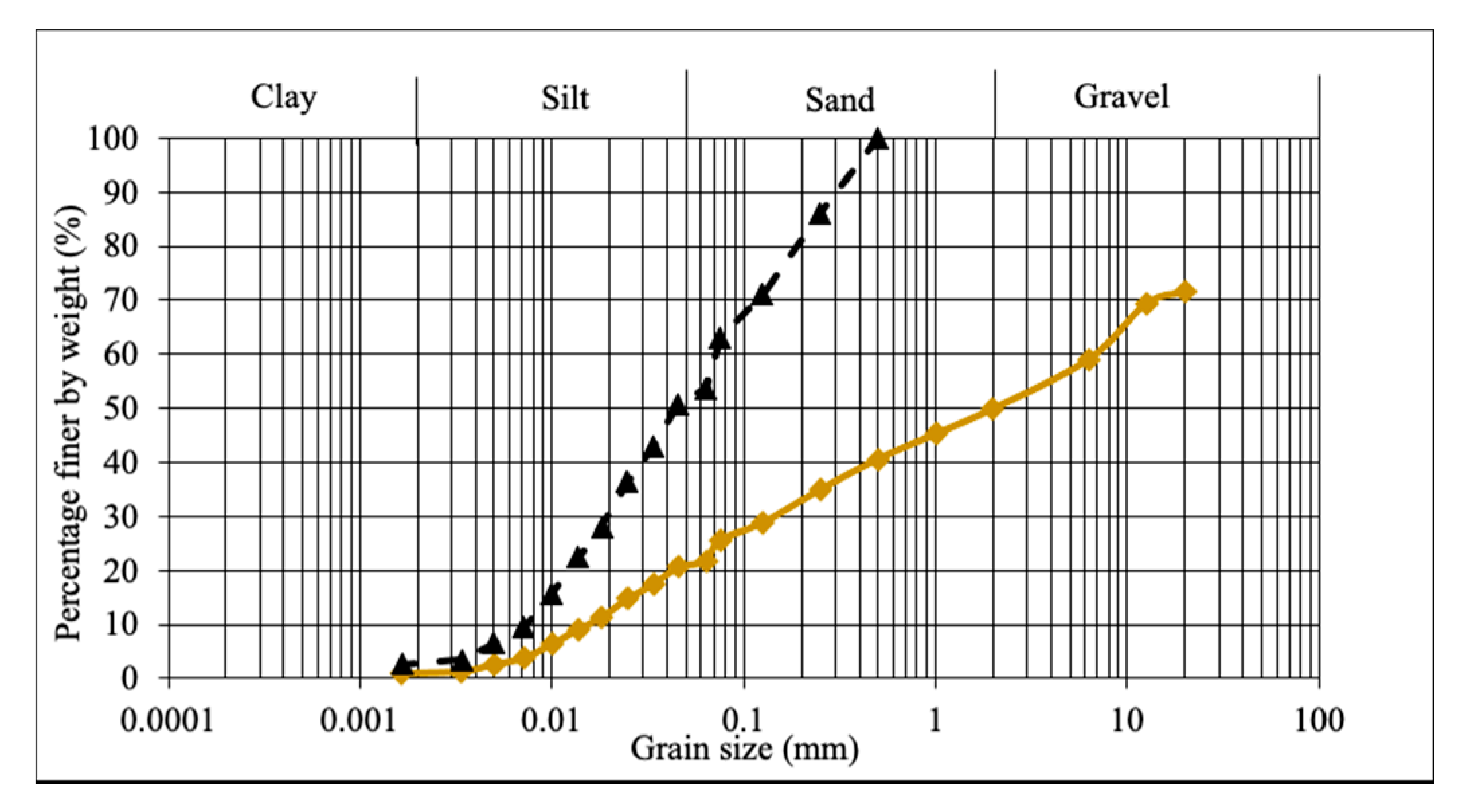
The investigated material comes from Illgraben catchments in Switzerland, where several floods are expected every year. The Illgraben catchment (10.4 km2) is located in the western part of Switzerland and extends from the summit of the Illhorn mountain (2716 m above sea level (asl)) to the fan apex (850 m asl) and to the outlet of the Illgraben into the River Rhone (610 m asl). A wide variety of flow types have been observed in Illgraben, ranging from granular to muddy debris flows, to hyperconcentrated flows and flood events [21,22]. Debris flows typically occur during intense summer thunderstorms from April to October. The tested material, which has been collected from the deposit areas along the channel, has a specific gravity of 2.633 and it is characterized by the presence of a coarse sediment fraction (80% sand-gravel and 20% silt-clay), as it is shown in Figure 1.
In order to prepare the testing samples, the collected soils were purified from the residual plants and organic matter, and were dried in an oven at 105 °C for a day. Subsequently, the fraction coarser than 0.5 mm was removed, and the volume dry sediments Vs, conveniently cooled, have been mixed with an appropriate volume of distilled water Vw in order to obtain a mixture having the desired sediment concentration C by volume:
Rheological measurements, consisting of sweep tests and creep tests, have been carried out using a commercial rotational rheometer MCR 301 manufactured by Anton Paar. The rheometer can work in both stress-controlled and rate-controlled modes. It has a range of torque of 10−7–0.2 Nm with a max accuracy of 2 × 10⁻⁷ Nm, and a rotational speed ranging from 10−6 1/min to 3 × 10³ 1/min.
The rheometer can operate with different geometries: concentric cylinder, double-gap measuring system, vane, cone-plate measuring system, parallel-plate measuring system or customized solution. Vane geometry was selected for the experiments. It consists of a four-bladed vane and a measuring cup. The cylinder defined by the tips of the blades has a radius of 11 mm and a length of 16 mm. The radius of the measuring cup is 14.46 mm.
The rotor is rotated around its axis at a given rotational speed and the torque T is measured. During the test the material was trapped in the blades and the shear was achieved around a fictitious cylinder within the mixture; as a consequence, the flow characteristics, to a first approximation, are similar to those of two solid coaxial cylinders, having an inner radius equal to the radius of the blades [23]. No slip was expected at the inner wall, since there is not any solid/mixture interface. The analyzed debris flow mixtures were tested in shear-controlled mode at constant temperature (23 °C). Preliminary tests were carried out to define the maximum shear to be applied without any spilling of the mixture from the measurement gap.
Stress sweep tests consisted of measuring the apparent flow curves by applying an increasing shear stress ramp. The shear stress was continuously increased in a logarithmic way from a minimum value (typically 0.1 Pa) to a maximum value depending on the sediment concentration of the mixture, and the corresponding shear rate was measured. The total duration of the sweep test was typically 60 s. The complete testing procedure consisted of setting up the material inside the geometry and imposing a pre-shear (typically, a constant shear rate at 600 1/s for 30 s) in order to homogenize the samples.
Creep experiments consisted of imposing a shear stress and recording the strain response in time. At stresses lower than the yield stress, yield stress materials behave like elastic solids, therefore the strain increases in time toward a constant value. Creep tests were carried out imposing a premixing at 600 1/s for 30 s to homogenize the mixture, and varying rest time up to 9 h. Shear stresses ranged from 40 to 1500 Pa depending on the grain concentration.
Sweep and creep tests have been carried out involving mixtures having different grain concentrations ranging between 50% and 58% by volume. Different initial conditions of the mixtures, such as homogenization and prior resting time (up to 9 h), were applied in order to analyze the effects of aging and rejuvenation (i.e., thixotropy).
3. Results
The reconstituted debris-flow mixtures at different solid concentrations show a yield stress fluid behavior, characterized by the presence of a static and dynamic yield stress associated with flow starting and stopping [19,24,25]. Recently Quian et al. [26] showed they are related to the microstructural material state, whereas Barnes and Walters [27] already pointed out the time dependent property of yield stress.
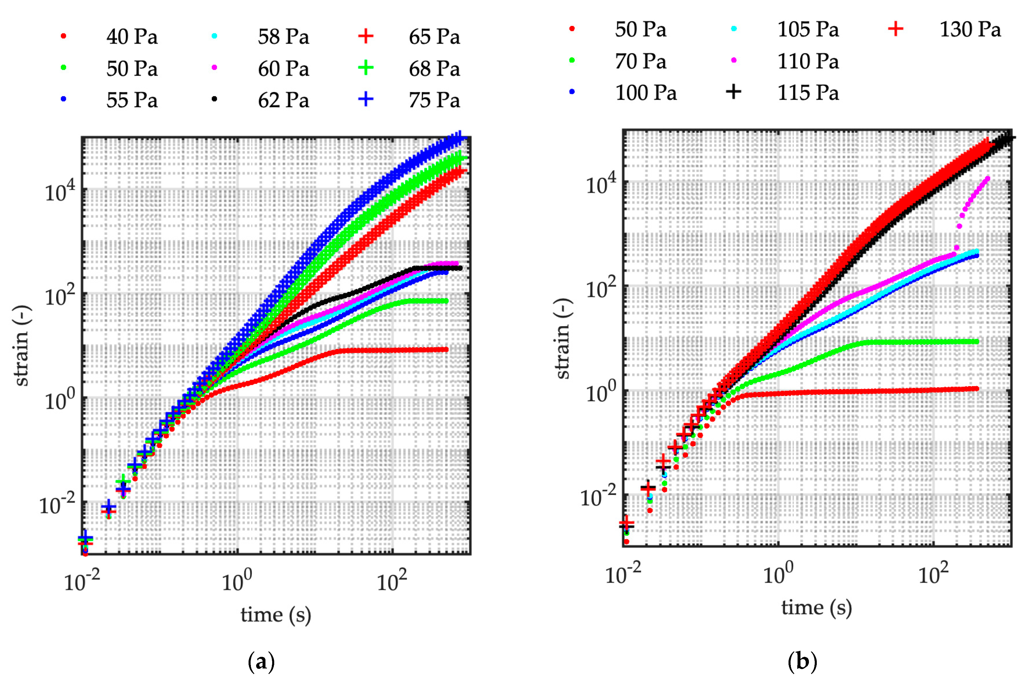
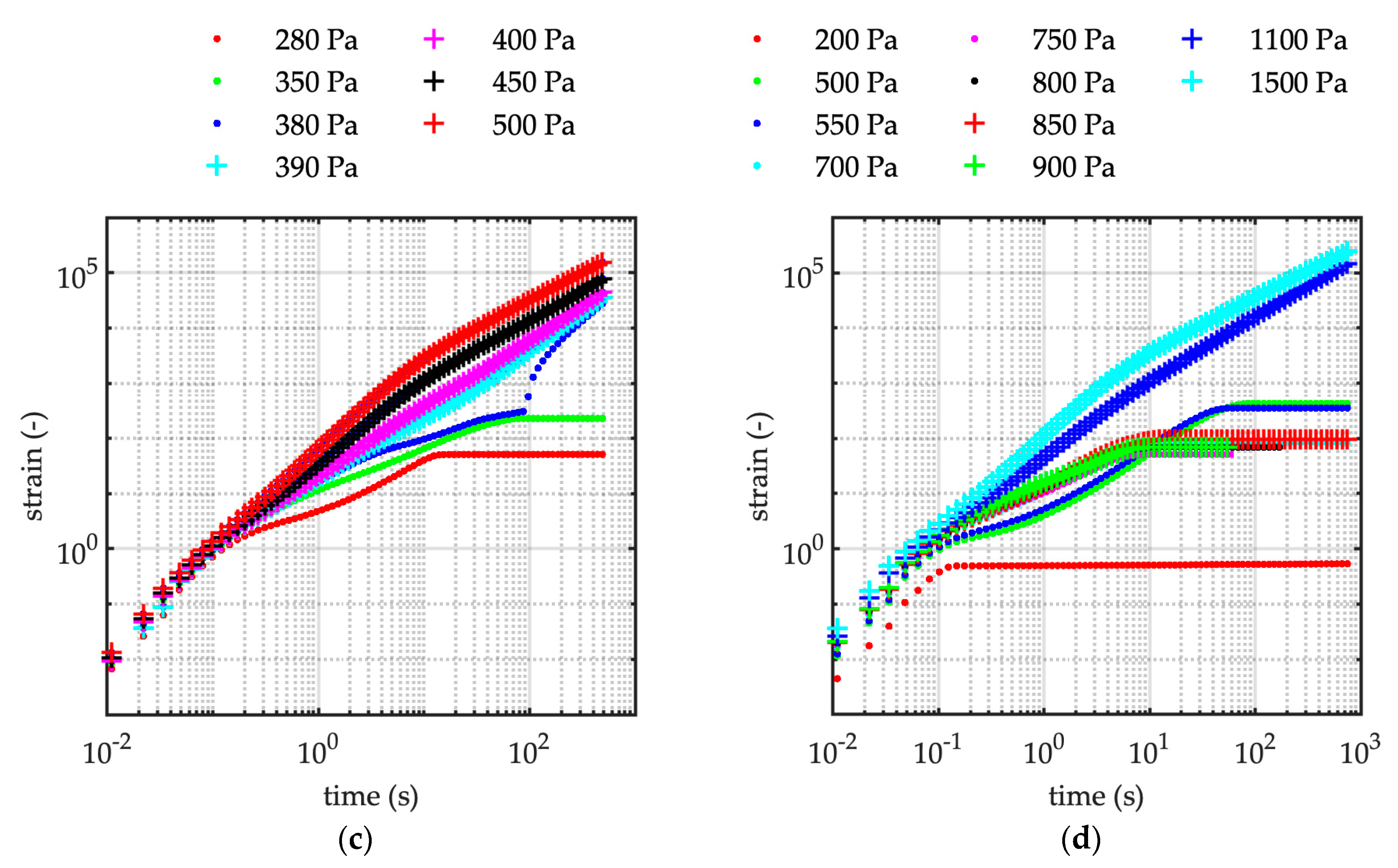
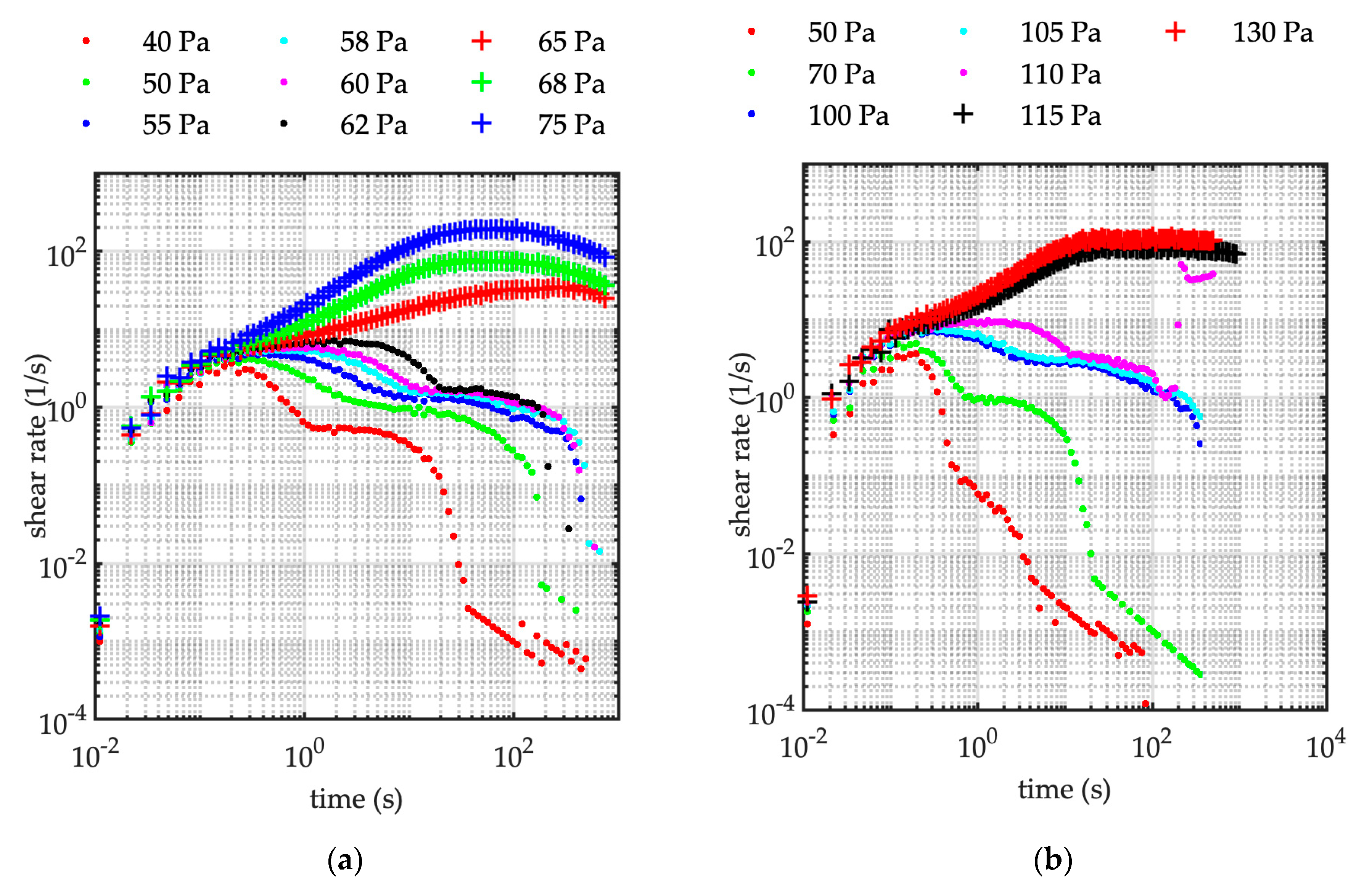
In Figure 2, Figure 3 and Figure 4 the results of the creep tests are plotted for different mixture’s sediment concentration, respectively, in terms of strain, shear rate and apparent viscosity on time.
Independently of the sediment concentration herein considered (i.e., ranging from 50% to 58%), the slurries behave as a yield stress fluid. It is consistent with other experimental results involving reconstituted debris-flow mixture, which also provided evidence that the yield stress depends on grain size and shape, grain concentration and fine particle content [14,28,29,30]. When the imposed stress is slightly smaller than the critical value, the strain increases in time till a constant value (Figure 2) is gained, and the viscosity tends to diverge to infinity (no steady state is reached), leading to the flowing stoppage of the mixture. Conversely, if the stress is slightly above the threshold value, the strain continuously increases in time, and the apparent viscosity tends to a constant value (Figure 4). Correspondingly, the shear rate tends to a constant value (Figure 3), as a consequence of a flowing steady state. Results are reported in Table 3; the threshold stress varies with sediment concentration, the higher the concentration the greater the threshold stress.
Coussot et al. [17] already pointed out it would be in striking contrast with the theoretical yield stress fluid, since the steady state viscosity abruptly changes from infinity to a finite value at the critical stress stage. It is worth noting, according to the experiments carried out with imposed shear stress, the mixture always presents an instability when the shear stress approaches its critical value. Corresponding to applied stress lower than its critical value, the apparent viscosity always shows a minimum at time 10−1–100 s (Figure 4), and it is associated with a low shear rate, which results in two order of magnitude lower than the shear rate corresponding to the flowing steady state regime (Figure 3).
Noticeably, independent of the grain concentration, corresponding to the lower applied shear stress (i.e., lower than threshold value), the viscosity initially increases in a range of 101–102 Pa⋅s, than after a short-period time (typically 101 s), the slurry suddenly halts and the viscosity tends to an infinite value. For stress higher than the critical value, the viscosity reduces over a short period of time of about 101 s, then shows a constant value corresponding to the ultimate flowing steady state (Figure 3).
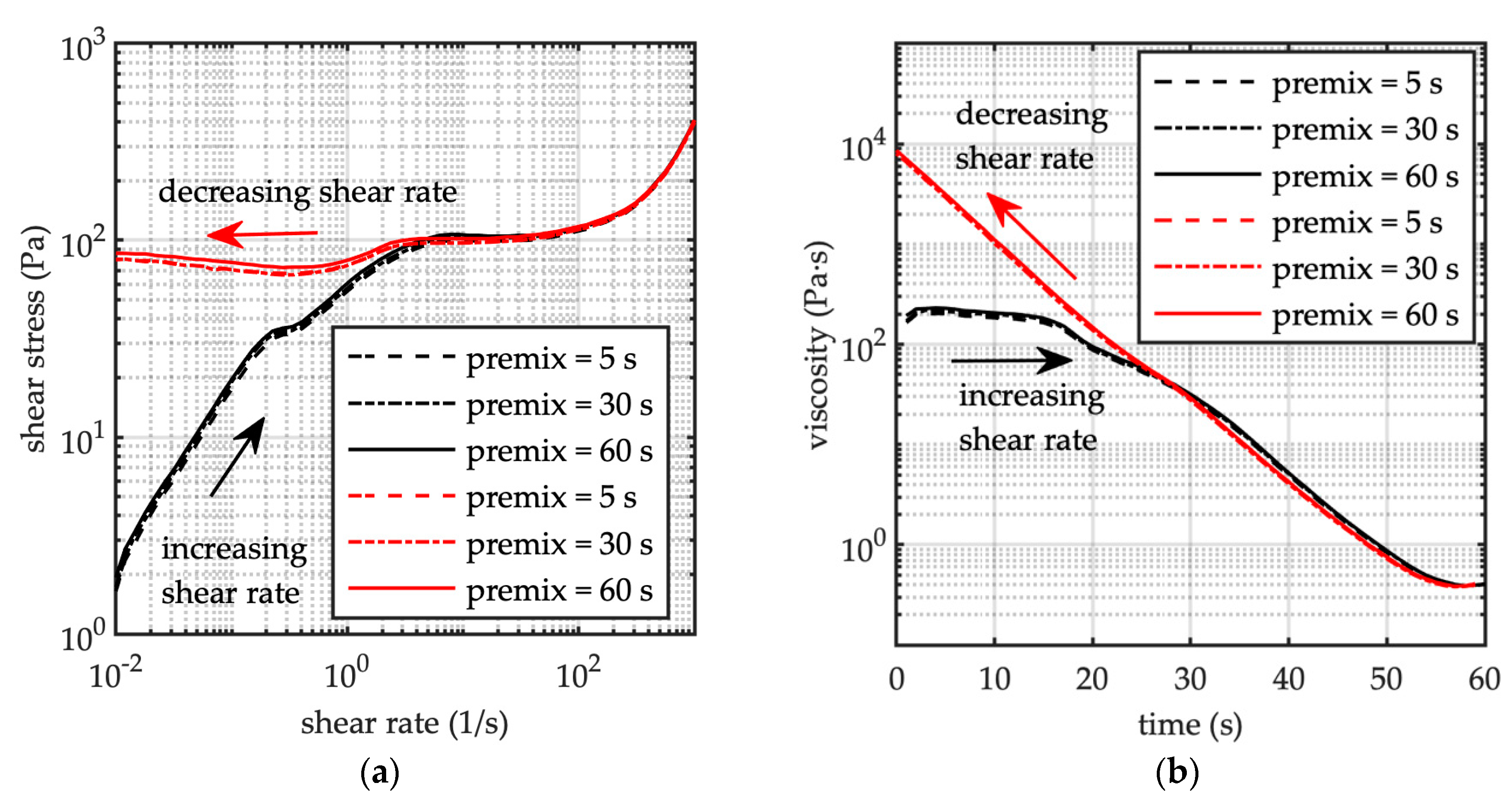
Consecutive flow tests have been carried out under rate-controlled mode, considering different premixing periods (i.e., 5, 30, 60 s) at a constant revolving speed (60 rpm), followed by a resting period of 5 s (i.e., tests F7, F8, and F9 see Table 1). Flow tests (Figure 5a) last 60 s during the increasing and decreasing shear ramp. Flow curves show a stress plateau, which is in fact an asymptotic case of the shear banding behavior [10]. In Figure 5b, for the sake of comprehension, the apparent viscosity is plotted as a function of the time, from 0 to 60 s (increasing ramp), and from 60 to 0 s (decreasing ramp). In every case the dynamic and static yield stress are the same, and the flow curves, corresponding to different premixing durations, overlap each other (see Figure 5a). It means that once the microstructure has been destroyed (after few seconds of pre-stirring), and the mixture does not have the possibility to experience an aging period, the mixture’s rheological behavior is the same, and it confirms the same viscosity evolution over time (Figure 5b).
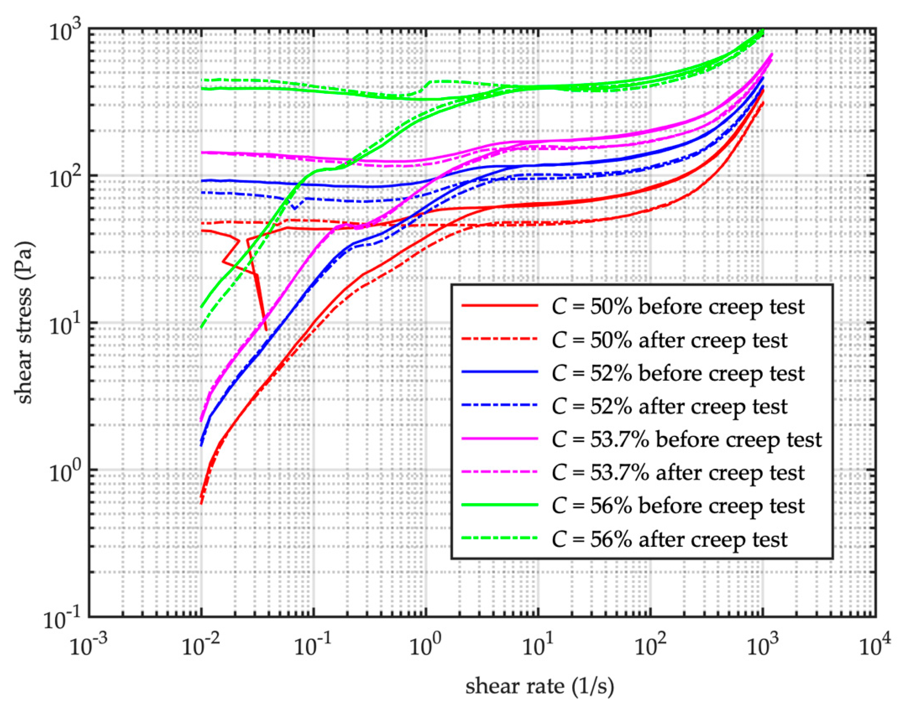
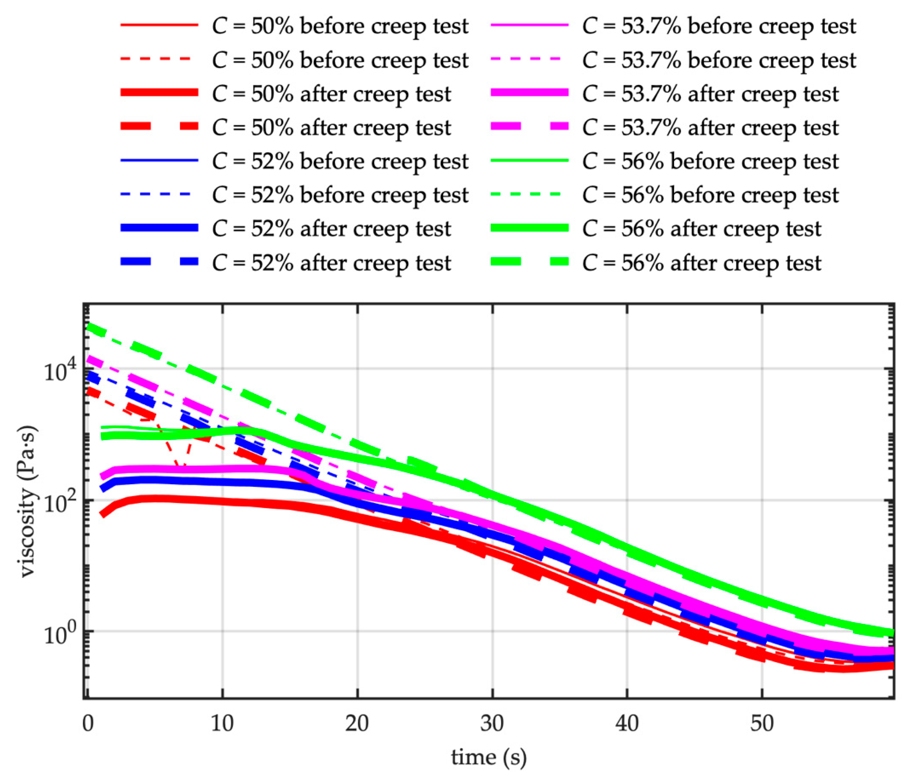
A different situation has been pointed out by performing flow tests, just before and after creep tests, varying sediment concentration of the tested mixtures. The creep tests are carried out increasing the applied shear stress (typically eight different values). Each creep test lasts about 1.5 h. Every flow test starts after a premixing period of 30 s, and subsequent rest period of 5 s. Figure 6 shows the flow curves before and after the creep test for different values of grain concentration. The apparent viscosity in the steady flow regime remains almost the same before and after the creep test (see Figure 7). For all the tested grain concentration, hysteresis effects are slightly evident, but the critical shear stress corresponding to the banding zone of the flow curves differs before and after creep tests, being the difference more evident in the case of lower concentration.
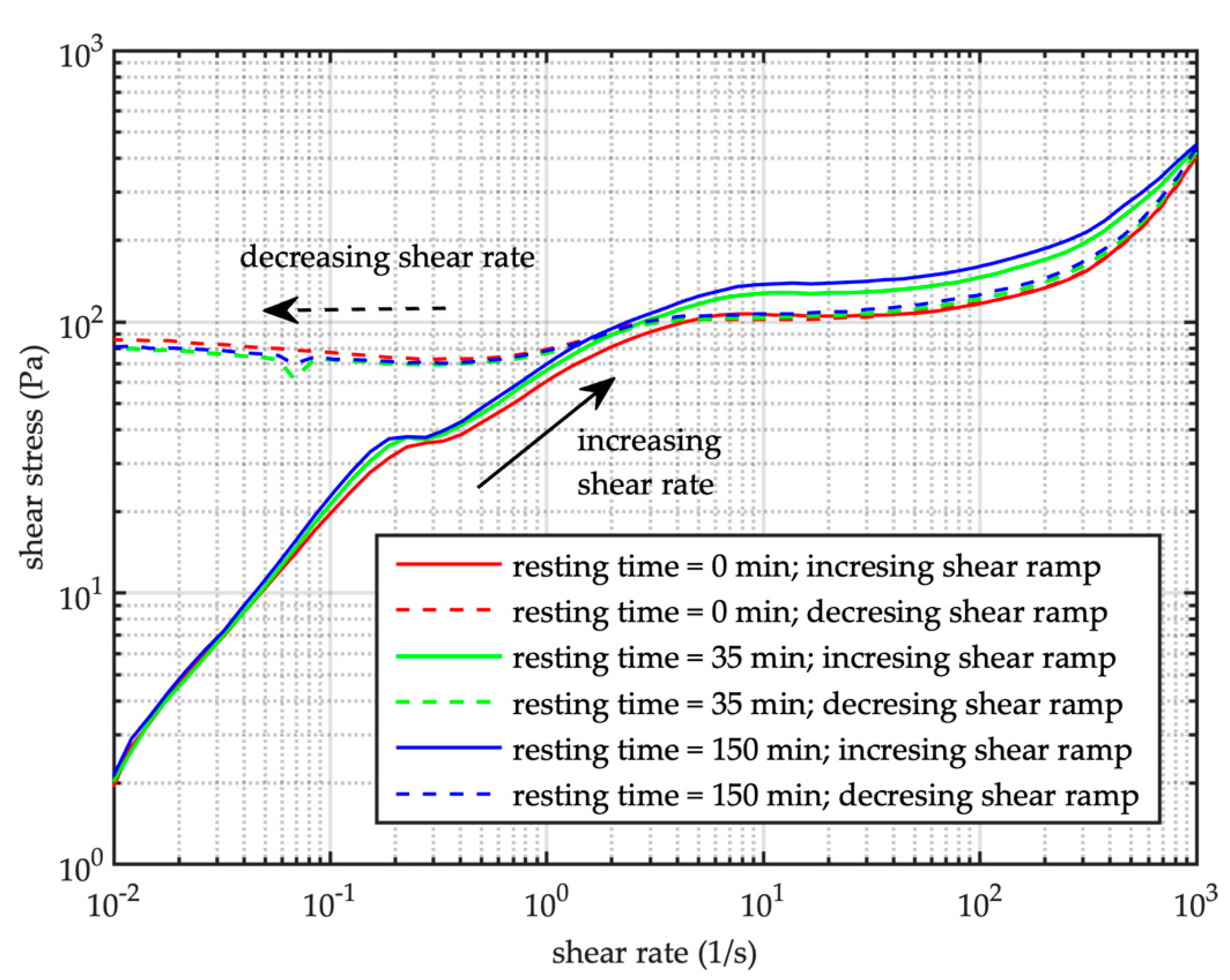
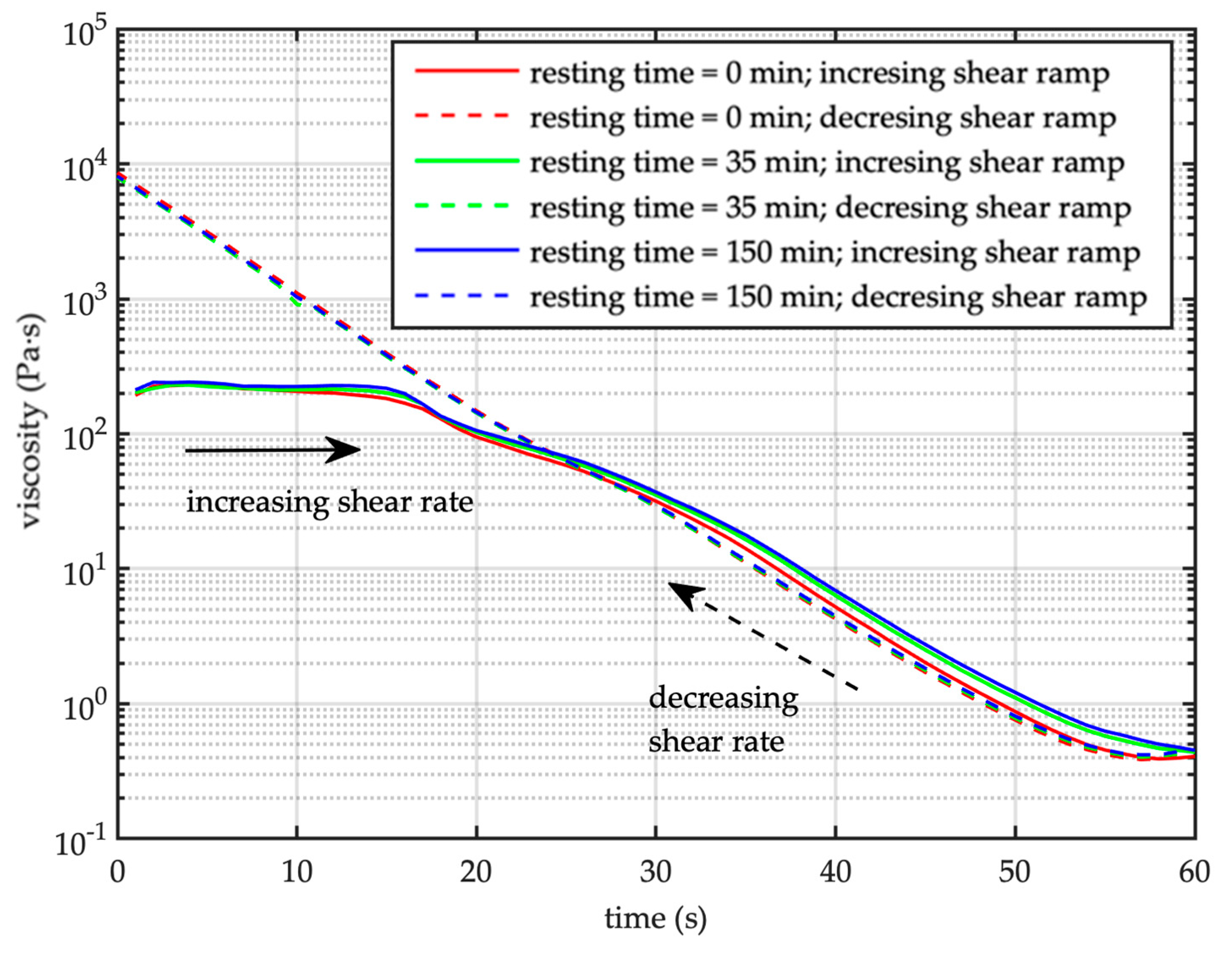
Flow curve tests F9, F10 and F11 were carried out using the same mixture (sediment concentration C = 52%) and increasing the resting time before each run (Figure 8). The first run (i.e., F9) was carried out pre-shearing the mixture for 60 s at a constant shear rate of 600 s−1 and keeping the mixture at rest 5 s before shearing. Then, the test starts following an increasing and decreasing shear rate ramp. At the end of the decreasing ramp the mixture rested for longer time (35 and 150 min between run F9–F10 and F10–F11, respectively) before it was stirred 5 s at = 600 s−1, and the next run started. Despite the resting period between the different runs, the mixture exhibits the same steady state apparent viscosity (Figure 9). The resting period affects the shear stress during the increasing shearing ramp. In effect, the longer the resting time, the higher the stress (Figure 8). The flow curves suggest a nonlinear behavior of the static yield stress with respect to resting time, along with an asymptotic trend for longer resting time. Corresponding to the decreasing shear ramp applied, the stress seems much less sensitive to the resting time, showing an almost complete overlapping. As a consequence, the dynamic yield stress and the viscosity rate are the same, no matter the resting period. The complete overlapping of the flux curves corresponding to the lower shear rate is remarkable (i.e., rate < 1–2 s−1).
The stress plateau found in the sweep test (see Figure 5 and Figure 6) indicates a typical yield stress fluid behavior, whereas the hysteresis indicates thixotropic behavior, as a consequence of resting time experienced by the mixtures. Thus, the slurry presents initially a more structured state, which leads to the apparent “static” yield stress, and after shearing, the apparent “dynamic” yield stress differs from the original “static” one. In this way, the time dependent shear stress response (along with the influence of sediment concentration already discussed) may be appreciated.
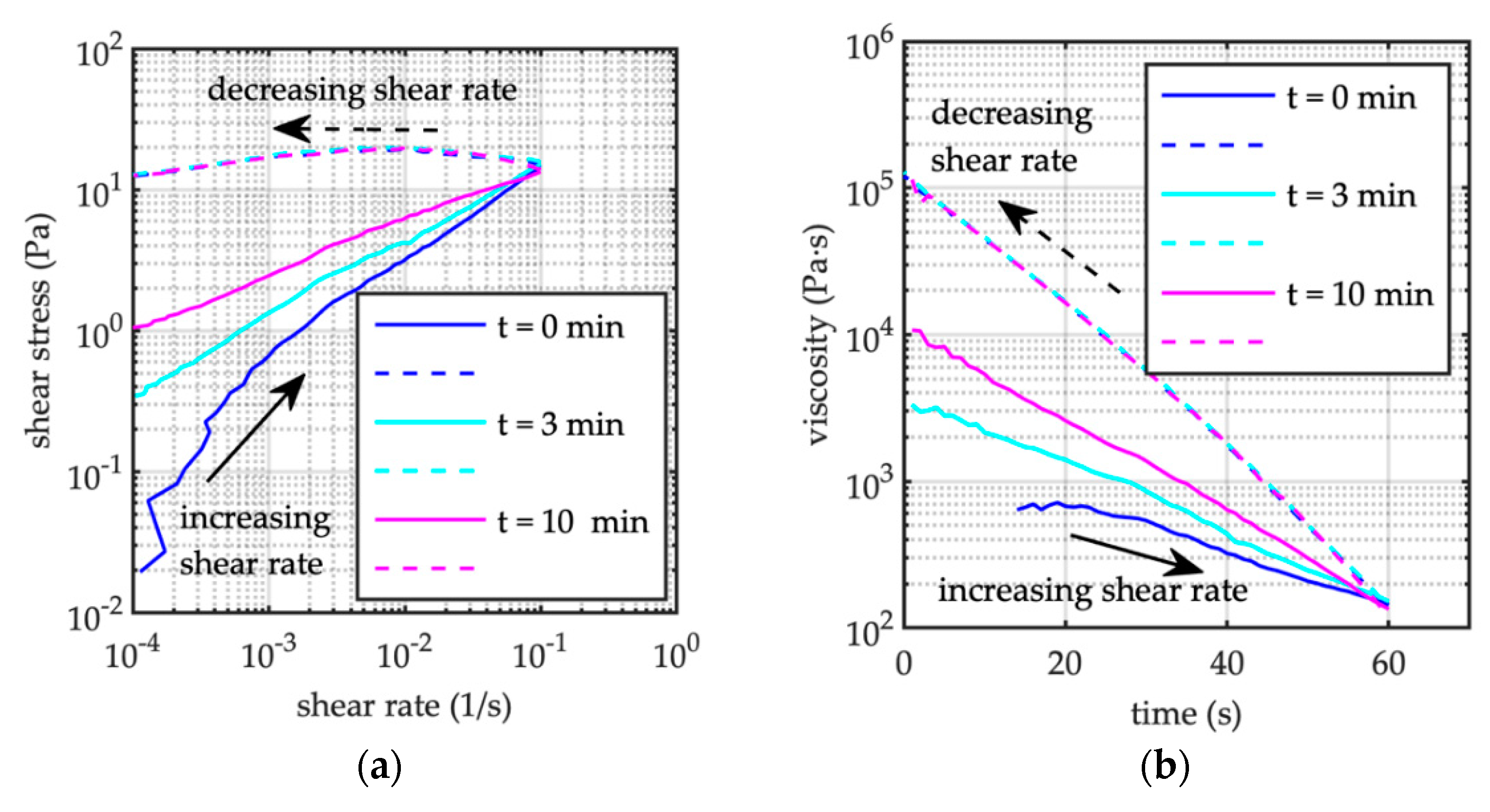
Runs F24, F25 and F26 were carried out to study the thixotropy behavior of the mixture having a sediment concentration C = 50%, sheared at very low shear rate (i.e., s−1) applying different resting times (0, 3, and 10 min, respectively, for runs F24, F25 and F26) after pre-stirring, just before running the test for 60 s. In any case, the mixture was pre-stirred at a constant shear rate = 600 s−1 for 30 s. The measured shear stress depends on the resting time: for instance, corresponding to a shear rate of 10−4 s−1, the shear stress varies over one order of magnitude increasing the resting time. Even in these cases referring to the increasing ramp, the longer the resting time, the higher the shear stress, whereas the flow curve completely overlapped during the decreasing shear ramp (Figure 10a), and the shear stress level remains almost the same (about 10–20 Pa, see Figure 10a), correspondingly the viscosity increase at the same rate by almost three orders of magnitude (Figure 10b).
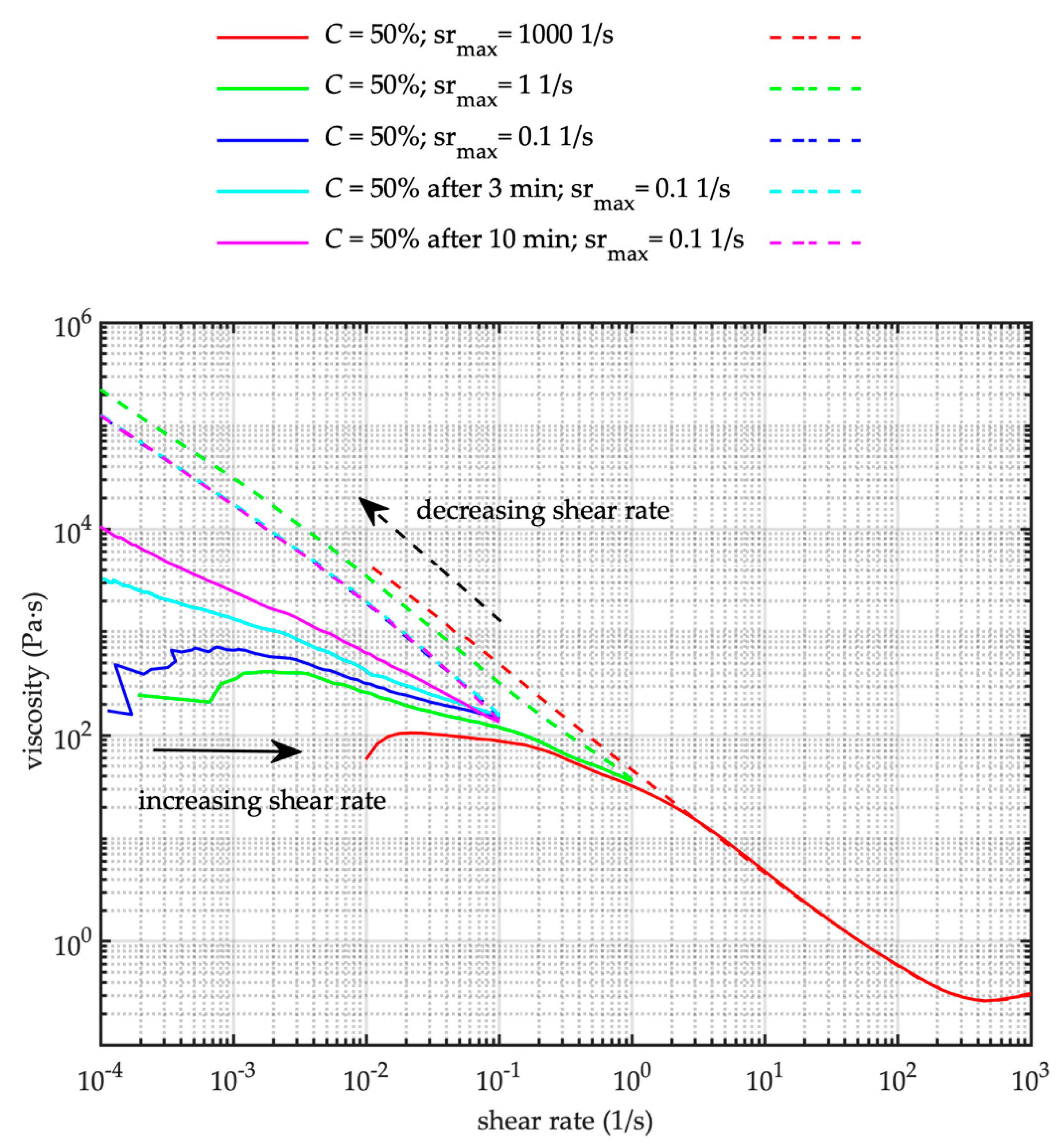
It is interesting to compare the flow curves at lower shear rate = [10−4, 10−1] s−1 (runs F24, F25, and F26) with the reference flow curve at higher shear rate run F22 = [10−2; 103] s−1 and run F23 = [10−4; 100] s−1. Runs F22 and F23 were carried out pre-stirring the mixture 30 s at a constant shear rate = 600 s−1 followed by a resting period of 5 s. Both tests lasted 60 s, with a semilogarithmic shear rate for the increasing ramp over time. The shear banding (run F22) occurs between about = 4 × 100 s−1 and = 101 s−1. Once the critical shear rate has been reached during run F22 (see Figure 11), the mixture starts flowing and the viscosity tends progressively to its steady state value. The static and dynamic shear stress values are the same (i.e., about 45 Pa). When the critical shear rate is not attained during the increasing ramp (i.e., < 4 × 100 s−1; run F23, F24, F25 and F26), the stress level remains lower than its critical value (i.e., about 45 Pa, run F22 in Figure 11), and during the following decreasing shear rate ramp the flow curve shows a plateau regime, thus the apparent viscosity reduces at the same rate, no matter the resting period between the subsequence tests (Figure 12). Interestingly, during the run F22, F23 and F24 the mixtures experienced the same initial viscosity of about 102 Pa⋅s, corresponding to the identical initial condition of the mixture (i.e., pre stirring of 30 s at = 600 s−1, 5 s resting time before flowing). When longer resting time is applied before flowing (i.e. runs F25 resting time of 3 min, and F26 resting time of 10 min) the initial viscosity increases over orders of magnitudes and no pseudo plateau regime appears. As far as the shear rate approaching its critical value , the viscosity tends to the same value, no matter the initial condition of the mixture (Figure 12).
The measurement of shear stress depends on the applied initial shear rate, as it is evident in Figure 11 comparing the F22 and F23 tests. The viscous plateau occurs (see Figure 12) independently on the initial applied shear rate (i.e., runs F22, F23 and F24) as it was already observed by Jeon [25], but it disappears as a consequence of aging due to a prolonged resting period.
4. Discussion
The experiments at imposed shear stress demonstrate that, corresponding to a shear stress higher than the threshold value, the mixtures behave as a conventional thixotropic mixture. In fact, viscosity decreases in time till it reaches a steady state constant value. For lower values of the imposed shear stress the mixture starts flowing, the strain initially increases (Figure 2), then the viscosity suddenly increases by several orders of magnitude (Figure 4), leading to a stoppage of the fluid. In this case, it is not possible to apply any equilibrium viscosity asset. In this sense the threshold shear stress value may be interpreted as a yield stress and the mixture may be considered as a yield stress fluid, and the flow like behavior of the mixture can be modeled as a generalized Herschel–Bulkley fluid, accounting for sediment concentration [14]. Indeed, the threshold stress value depends on sediment concentration, and creep test’s curves are qualitatively the same no matter the grain content.
Flow curve experiments show the rheological behavior is not affected by the pre-shearing period (see Figure 5a,b), it means once the original structure has been destroyed (after few seconds of pre-stirring), the viscosity decreases over time till a steady-state constant value has been reached (Figure 5b).
Nonetheless the stress–strain history of the mixture affects its rheological behavior. In fact, flow curve experiments alternated with creep tests (Figure 6) show different static and dynamic yield stress values, the difference being more relevant at lower grain concentration. The creep test affects the microstructure network and fosters the rejuvenation of the mixture, in fact the stress level is higher before than after creep test, and grain concentration enhanced the microstructure, reducing the effect of rejuvenation. On the contrary, the ultimate viscosity corresponding to the steady state fluid-like behavior remains the same for the tests carried out before and after creep tests, being the steady state viscosity value function of granular concentration (see Figure 7).
Long resting time very much affects the rheological behavior of the mixture in terms of static yield stress; on the contrary the dynamic yield stress almost remains the same independently of the resting period. Longer periods of rest make the rearrangement of the microstructure more effective, which is responsible of the abrupt change from stop to flowing, even because of the role of the gravity, despite the pre-stirring applied before starting the tests. The shearing flow tends to the same steady-state viscosity value (see Figure 9), independently of the resting period herein applied. After the microstructure has been destroyed during the flowing phase, decreasing the shear rate leads the mixture to experience the same aging and it results on the same dynamic yield stress, no matter the imposed resting period in the beginning of the experiments.
At low shear rate, the different aging state, corresponding to different resting times of the mixture, afflicts the initial part of the flow curves (i.e., the increasing shear ramp), the longer the period of rest the higher the apparent viscosity (see Figure 11 and Figure 12). Nonetheless, the rejuvenation progressively leads to the same flow curve independently of the resting time (or aging level), and in this case corresponding to the maximum imposed shear ( < 10−1 s−1) the different aged mixtures experience the same apparent viscosity η ≈ 1.5 × 10² Pa⋅s, which is much larger than the steady state viscosity η ≈ 3 × 10⁻¹ Pa⋅s (test F22 in Figure 12). The descending shear rate curve gives the same stress–strain response no matter the former aging level (Figure 11). Interestingly, the stress level remains almost constant during the reducing shear rate ramp, and it is lower than the dynamic yield.
In the case of test F23, the applied maximum shear rate is higher than in tests F24, F25 and F26. It means the mixtures experienced a further level of rejuvenation, which reduces the viscosity during the increasing shearing ramp of flow, even though it remains higher than the steady state viscosity value by two orders of magnitude (Figure 12). It may be considered that the rejuvenation state was not enough developed to completely break the microstructure as it is when the critical stress–strain level is obtained (in this case a critical shear rate higher than = 101 s−1 corresponding to yield stress of about 45 Pa) and the shear stress necessary to completely halt the flowing slurry is lower than the threshold yield stress. In this way, it is possible to indicate three different regimes; a lower shear rate regime, corresponding to a shear rate lower than the critical value , in which the increasing shear rate promotes the motion of the slurry, showing viscosity values larger than steady state value by order of magnitude; an intermediate unstable shear rate regime, corresponding to a shear rate , in which the mixtures show a shear banding behavior characterized by yield stress level; and a higher shear rate regime for , where the flowing debris behave as a non-Newtonian fluid characterized by a constant steady state viscosity. The rheological behavior of these three regimes is affected by the initial condition of the mixture, and whereas the ultimate steady state viscosity is not affected by the initial condition. In particular, the long-term period of rest leads to hysteresis on the flow curve, with a distinct dynamic and static yield stress. Eventually the experiments provide evidence of the role of grain concentration on the rheology of the reconstituted debris-flow mixtures.
5. Conclusions
Reconstituted real debris-flow samples have been tested using a rotational standard rheometer, varying sediment concentration, premixing duration, resting period and test procedures (sweep tests and creep tests).
Tested slurries show viscosity bifurcation and yield stress behavior. Accounting for a fixed long-term aging period, once the mixture has been stressed till the microstructures have been destroyed (in this case after few seconds of pre-stirring), the rheological behavior of the flowing mixture is independent of the duration of the stress applied to destroy the microstructure (i.e., on the duration of pre-stirring). It suggests a threshold level for the aging/rejuvenation asset.
The stress–strain history of the mixture affects the rheometric response in terms of yield stress, the lower the grain content the higher the effects. Rejuvenation of the mixture reduces the static and dynamic yield stress, and grain concentration enhanced the microstructure lowering the effect of rejuvenation. On the other hand, increasing the long-term aging period (i.e., increasing the resting time) leads to higher static yield stress, the steady state flowing behavior and the dynamic yield being almost the same. The longer the long-term aging the higher the increase in the static yield. At lower shear rate, the different aging state afflicts the initial part of the flow curves. The higher the sediment concentration, the higher the stress. Nonetheless, the rejuvenation progressively leads to the same stress–strain relationship independently of the aging level.
In any case, the initial condition of the mixture (i.e., the microstructure organization) and the sediment concentration affect both the time-dependent (thixotropy) slurries behavior and the ultimate steady state rheology.
On these bases it is possible to highlight the macroscopic effects of aging-rejuvenation corresponding to the three different regimes: (1) a lower shear rate regime, where the shear rate is lower than the critical value , in which the flowing slurry shows an apparent viscosity much larger than steady state value. Apparent viscosity is variable with the shear, and the longer the aging period the higher the stress level and the viscosity. Approaching to critical shear rate , the mixture tends to a static yield stress value, which depends on the aging of the mixture. (2) An intermediate banding shear rate regime characterized by static and dynamic yield stress level. The aging of the mixture increases the static yield stress, and the lower the grain concentration the more evident the hysteresis. On the contrary the dynamic yield stress remains almost independent on the aging-rejuvenation experienced by the mixture. (3) A higher shear rate regime, where the flowing debris behaves as a non-Newtonian fluid characterized by a constant steady state ultimate apparent viscosity. In this regime the ultimate viscosity remains a function of the grain concentration, but it is independent of the time history of the mixture.
The results suggest that in the field not only the change in granular concentration (e.g., related to rainfall event) may cause a reduction of static yield stress, leading to a rapid flow associated with a shear rate greater than the critical value, but also that the slurry may change rheological properties because of rejuvenation experienced during the flowing state. Accordingly, it reduces dynamic yield stress, and may cause the stoppage of the material on a milder slope, providing a longer distance of the flowing material. Further studies should be oriented to better understand the role of gravity, which fosters grain sedimentation (over a short and long-time scale) and afflicts density homogeneity of the mixtures, which in turn may influence the time variability of rheological behavior.
Author Contributions
Conceptualization, L.S. and F.D.; methodology L.S., F.D. and A.M.P.; validation, L.S. and F.D.; formal analysis, L.S., A.M.P.; investigation, L.S., A.M.P. and E.P.; data curation, A.M.P., E.P. and L.S.; writing—original draft preparation, L.S.; writing—review and editing, L.S. and F.D.; visualization, L.S.; supervision, L.S., and F.D. All authors have read and agreed to the published version of the manuscript.
Funding
This research received no external funding.
Data Availability Statement
The data presented in this study are available on request from the corresponding author (it is mandatory to cite the present paper when the data are used).
Conflicts of Interest
The authors declare no conflict of interest.
References
- Barnes, H.A. Thixotropy a review. Non-Newton. Fluid Mech. 1997, 70, 1–33. [Google Scholar] [CrossRef]
- Barnes, H.A. The yield stress a review or ‘panta rei’ everything flows? Non-Newton. Fluid Mech. 1999, 81, 1–33. [Google Scholar] [CrossRef]
- Mueth, D.M.; Debregeas, G.F.; Karczmar, G.S.; Eng, P.J.; Nagel, S.R.; Jaeger, H.M. Signatures of granular microstructure in dense shear flows. Nature 2000, 406, 385–389. [Google Scholar] [CrossRef] [PubMed] [Green Version]
- Huang, N.; Ovarlez, G.; Bertrand, F.; Rodts, S.; Coussot, P.; Bonn, D. Flow of wet granular materials. Phys. Rev. Lett. 2005, 94, 028301. [Google Scholar] [CrossRef] [PubMed] [Green Version]
- Pellegrino, A.M.; Schippa, L. Macro viscous regime of natural dense granular mixtures. Int. J. Geomate 2013, 4, 482–489. [Google Scholar] [CrossRef]
- Ovarlez, G.; Bertrand, F.; Rodts, S. Local determination of the constitutive law of a dense suspension of noncolloidal particles through MRI. J. Rheol. 2006, 50, 259–292. [Google Scholar] [CrossRef] [Green Version]
- Barnes, H.A.; Hutton, J.F.; Walters, K. An Introduction to Rheology; Elsevier: Amsterdam, The Netherland, 1989. [Google Scholar]
- Contreras, S.M.; Davies, T.R.H. Coarse-grained debris flows, hysteresis and time-dependent rheology. J. Hydraul. Eng. 2000, 126, 938–941. [Google Scholar] [CrossRef]
- Fall, A.; Bertrand, F.; Ovarlez, G.; Bonn, D. Yield stress and shear-banding in granular suspensions. Phys. Rev. Lett. 2009, 103, 178301. [Google Scholar] [CrossRef] [Green Version]
- Ovarlez, G.; Rodts, S.; Chateau, X.; Coussot, P. Phenomenology and physical origin of shear localization of the shear banding in complex fluids. Rheol. Acta 2009, 48, 831–844. [Google Scholar] [CrossRef] [Green Version]
- Chen, H.; Lee, C.F. Runout analysis of slurry flows with Bingham model. J. Geotech. Geoenviron. Eng. 2002, 128, 1032–1042. [Google Scholar] [CrossRef]
- Jeon, S.W.; Leroueil, S.; Locat, J. Applicability of power law for describing the rheology of soils of different origins and characteristics. Can. Geotech. J. 2009, 46, 1011–1023. [Google Scholar] [CrossRef]
- Schippa, L.; Pavan, S. Numerical modelling of catastrophic events produced by mud or debris flows. Int. J. Saf. Secur. Eng. 2011, 1, 403–423. [Google Scholar] [CrossRef]
- Schippa, L. Modeling the effect of sediment concentration on the flow-like behavior of natural debris flow. Int. J. Sediment Res. 2020, 35, 315–327. [Google Scholar] [CrossRef]
- Pellegrino, A.M.; Scotto Di Santolo, A.; Schippa, L. The sphere drag rheometer: A new instrument for analysing mud and debris flow materials. Int. J. Geomate 2016, 11, 2512–2519. [Google Scholar] [CrossRef]
- Pellegrino, A.M.; Scotto Di Santolo, A.; Schippa, L. An integrated procedure to evaluate rheological parameters to model debris flows. Eng. Geol. 2015, 196, 88–98. [Google Scholar] [CrossRef]
- Coussot, P.; Nguyen, Q.D.; Huynh, H.T.; Bonn, D. Viscosity bifurcation in thixotropic, yielding fluids. J. Rheol. 2002, 46, 573–589. [Google Scholar] [CrossRef] [Green Version]
- Coussot, P.; Nguyen, Q.D.; Huynh, H.T.; Bonn, D. Avalanche Behavior in Yield Stress Fluids. Phys. Rev. Lett. 2002, 88, 175501. [Google Scholar] [CrossRef] [Green Version]
- Pellegrino, A.M.; Schippa, L. Rheological modeling of macro viscous Flows of granular suspension of regular and irregular particles. Water 2018, 10, 21. [Google Scholar] [CrossRef] [Green Version]
- Pellegrino, A.M.; Schippa, L. A laboratory experience on the effect of grains concentration and coarse sediment on the rheology of natural debris-flows. Environ. Earth Sci. 2018, 77, 749. [Google Scholar] [CrossRef]
- Badoux, A.; Graf, C.; Rhyner, J.; Kuntner, R.; McArdell, B.W. A debris-flow alarm system for the Alpine Illgraben catchment: Design and performance. Nat. Hazards 2009, 49, 517–539. [Google Scholar] [CrossRef] [Green Version]
- Bennet, G.L.; Molnar, P.; McArdell, B.W.; Schlunegger, F.; Burlando, P. patterns and control of sediment production, transfer and yield in Illgraben. Geomorphology 2013, 188, 68–82. [Google Scholar] [CrossRef]
- Nguyen, Q.D.; Boger, D.V. Direct yield stress measurement with the vane method. J. Rheol. 1985, 29, 335–347. [Google Scholar]
- Scotto Di Santolo, A.; Pellegrino, A.M.; Evangelista, A.; Coussot, P. Rheological behaviour of reconstituted pyroclastic debris flow. Géotechnique 2012, 62, 19–27. [Google Scholar] [CrossRef]
- Jeong, S.W. Shear Rate-Dependent Rheological Properties of Mine Tailings: Determination of Dynamic and Static Yield Stresses. Appl. Sci. 2019, 9, 4744. [Google Scholar] [CrossRef] [Green Version]
- Qian, Y.; Kawashima, S. Distinguishing dynamic and static yield stress of fresh cement mortars through thixotropy. Cem. Concr. Comp. 2018, 86, 288–296. [Google Scholar] [CrossRef]
- Barnes, H.A.; Walters, K. The yield stress myths? Rheol. Acta 1985, 24, 323–326. [Google Scholar] [CrossRef]
- Schatzmann, M.; Fischer, P.; Bezzolla, G.R. Rheological behaviour of fine and large particle suspensions. J. Hydraul. Eng. 2003, 129, 796–803. [Google Scholar] [CrossRef]
- Kaitna, R.; Palucis, M.C.; Yohannes, B.; Hill, K.M.; Dietrich, W.E. Effects of coarse grain size distribution and fine particle content on pore fluid pressure and shear behavior in experimental debris flows. J. Geophys. Res. Earth Surf. 2016, 121, 415–441. [Google Scholar] [CrossRef] [Green Version]
- Jeong, S.W. Grain size dependent rheology on the mobility of debris flows. Geosci. J. 2010, 14, 359–369. [Google Scholar] [CrossRef]
Figure 1.
Grain size distribution. (—) original collected samples. (- -) tested samples obtained from the original samples after separating the grain fraction larger than 0.5 mm.
Figure 1.
Grain size distribution. (—) original collected samples. (- -) tested samples obtained from the original samples after separating the grain fraction larger than 0.5 mm.

Figure 2.
Creep tests. The time–strain trend during the test. (a) Sediment concentration C = 50%. Runs C87–C95 (see Table 2) corresponding to the increasing applied shear as it is reported in the legend. (b) Sediment concentration C = 52%. Runs C36–C42 (see Table 2) corresponding to the increasing applied shear as it is reported in the legend. (c) Sediment concentration C = 56%. Runs C59–C65 (see Table 2) corresponding to the increasing applied shear as it is reported in the legend. (d) Sediment concentration C = 58%. Runs C96–C104 and Run C108 (see Table 2) corresponding to the increasing applied shear as it is reported in the legend.


Figure 3.
Creep test. The shear-time trend during the test. (a) Sediment concentration C = 50%. Runs C87–C95 (see Table 2) corresponding to the increasing applied shear as it is reported in the legend. (b) Sediment concentration C = 52%. Runs C36–C42 (see Table 2) corresponding to the increasing applied shear as it is reported in the legend. (c) Sediment concentration C = 56%. Runs C59–C65 (see Table 2) corresponding to the increasing applied shear as it is reported in the legend. (d) Sediment concentration C = 58%. Runs C96–C104 and Run C108 (see Table 2) corresponding to the increasing applied shear as it is reported in the legend.


Figure 4.
Creep test. The apparent viscosity-time trend during the test. (a) Sediment concentration C = 50%. Runs C87–C95 (see Table 2) corresponding to the increasing applied shear as it is reported in the legend. (b) Sediment concentration C = 52%. Runs C36–C42 (see Table 2) corresponding to the increasing applied shear as it is reported in the legend. (c) Sediment concentration C = 56%. Runs C59–C65 corresponding to the increasing applied shear as it is reported in the legend. (d) sediment concentration C = 58%. Runs C96–C104 and Run C108 (see Table 2) corresponding to the increasing applied shear as it is reported in the legend.


Figure 5.
C = 52%. (a) Flow curves after different premixing period (runs F8, F7, F9—see Table 1—in the legend from the top to the bottom). (b) Viscosity over time for the same runs. Black line: increasing shear ramp (time = 0–60 s); red line: decreasing shear ramp (time = 60–0 s).
Figure 5.
C = 52%. (a) Flow curves after different premixing period (runs F8, F7, F9—see Table 1—in the legend from the top to the bottom). (b) Viscosity over time for the same runs. Black line: increasing shear ramp (time = 0–60 s); red line: decreasing shear ramp (time = 60–0 s).

Figure 6.
Flow curves before and after creep test, for different value of grain concentration C (runs F21, F22, F5, F6, F14, F15, F18, F19—see Table 1—in the legend from the top to the bottom).
Figure 6.
Flow curves before and after creep test, for different value of grain concentration C (runs F21, F22, F5, F6, F14, F15, F18, F19—see Table 1—in the legend from the top to the bottom).

Figure 7.
Apparent viscosity derived from the flow curves. Tests carried out before and after creep test, for different value of grain concentration C (runs F21 and F22, F5 and F6, F14 and F15, F18 and F19—see Table 1—in the legend from the top to the bottom). — increasing shear ramp (time 0–60 s); - - decreasing shear ramp (time 60–0 s).

Figure 8.
Flow curves (C = 52%) after different resting times (runs F9, F10, F11 in the legend from the top to the bottom).
Figure 8.
Flow curves (C = 52%) after different resting times (runs F9, F10, F11 in the legend from the top to the bottom).

Figure 9.
Apparent viscosity derived from the flow curves (C = 52%) after different resting times (runs F9, F10, F11 in the legend from the top to the bottom). — increasing shear ramp (time 0–60 s); - - decreasing shear ramp (time 60–0 s).
Figure 9.
Apparent viscosity derived from the flow curves (C = 52%) after different resting times (runs F9, F10, F11 in the legend from the top to the bottom). — increasing shear ramp (time 0–60 s); - - decreasing shear ramp (time 60–0 s).

Figure 10.
Sediment concentration C = 50%. Low shear rate tests after different resting times. Runs F24 (t = 0 min, reference test), F25 (after resting time of t = 3 min) and F26 (after resting time of t = 10 min). (a) Flow curves. (b) Apparent viscosity. — increasing shear ramp (time 0–60 s); - - decreasing shear ramp (time 60–0 s).

Figure 11.
Sediment concentration C = 50%. Flow curves at low shear rate after different resting times (F23, F24, F25 and F26) compared to the reference flow curve test (F22). Runs F22, F23, F24, F25 and F26 (from the top to the bottom of the legend). srmax indicates the maximum shear rate during the test; each test lasts 60 s). — increasing shear ramp; - - decreasing shear ramp.

Figure 12.
Apparent viscosity derived from the flow curve. Sediment concentration C = 50%. Flow curves at low shear rate after different resting times (F23, F24, F25 and F26) compared to the reference flow curve test (F22). Runs F22, F23, F24, F25 and F26 (from the top to the bottom of the legend). srmax indicates the maximum shear rate during the test. — increasing shear ramp (time 0–60 s); - - decreasing shear ramp (time 60–0 s).


Table 1.
Sweep tests summary.
| Runs | Sediment Concentration % | Premixing Period (s) | Resting Time (s) | Shear Rate (1/s) |
|---|---|---|---|---|
| F5 | 52 | 30 | 5 | 10−2–103 |
| F6 | 52 | 30 | 5 | 10−2–103 |
| F7 | 52 | 30 | 5 | 10−2–103 |
| F8 | 52 | 5 | 5 | 10−2–103 |
| F9 | 52 | 60 | 5 | 10−2–103 |
| F10 | 52 | 5 | 2.1 × 10³ (*) | 10−2–103 |
| F11 | 52 | 5 | 9.0 × 10³ (**) | 10−2–103 |
| F14 | 54 | 30 | 5 | 10−2–103 |
| F15 | 54 | 30 | 5 | 10−2–103 |
| F18 | 56 | 30 | 5 | 10−2–103 |
| F19 | 56 | 30 | 5 | 10−2–103 |
| F21 | 50 | 30 | 5 | 10−2–103 |
| F22 | 50 | 30 | 5 | 10−2–103 |
| F23 | 50 | 30 | 5 | 10−4–100 |
| F24 | 50 | 30 | 5 | 10−4–10−1 |
| F25 | 50 | 30 | 180 | 10−4–10−1 |
| F26 | 50 | 30 | 600 | 10−4–10−1 |
(*) Resting time between the end of run F9 and the beginning of the subsequent run F10. (**) Resting time between the end of run F10 and the beginning of the subsequent run F11.
Table 2.
Creep tests summary.
| Runs | Sediment Concentration % | Premixing Period (s) | Resting Time (s) | Shear Stress (Pa) |
|---|---|---|---|---|
| C36 | 52 | 30 | 10 | 50 |
| C37 | 52 | 30 | 10 | 70 |
| C38 | 52 | 30 | 10 | 100 |
| C39 | 52 | 30 | 10 | 105 |
| C40 | 52 | 30 | 10 | 110 |
| C41 | 52 | 30 | 10 | 130 |
| C42 | 52 | 30 | 10 | 115 |
| C59 | 56 | 30 | 10 | 280 |
| C60 | 56 | 30 | 10 | 350 |
| C61 | 56 | 30 | 10 | 380 |
| C62 | 56 | 30 | 10 | 390 |
| C63 | 56 | 30 | 10 | 400 |
| C64 | 56 | 30 | 10 | 450 |
| C65 | 56 | 30 | 10 | 550 |
| C87 | 50 | 30 | 10 | 40 |
| C88 | 50 | 30 | 10 | 50 |
| C89 | 50 | 30 | 10 | 55 |
| C90 | 50 | 30 | 10 | 58 |
| C91 | 50 | 30 | 10 | 60 |
| C92 | 50 | 30 | 10 | 62 |
| C93 | 50 | 30 | 10 | 65 |
| C94 | 50 | 30 | 10 | 68 |
| C95 | 50 | 30 | 10 | 75 |
| C96 | 58 | 30 | 10 | 200 |
| C97 | 58 | 30 | 10 | 500 |
| C98 | 58 | 30 | 10 | 550 |
| C99 | 58 | 30 | 10 | 700 |
| C100 | 58 | 30 | 10 | 750 |
| C101 | 58 | 30 | 10 | 800 |
| C102 | 58 | 30 | 10 | 850 |
| C103 | 58 | 30 | 10 | 900 |
| C104 | 58 | 30 | 10 | 1100 |
| C108 | 58 | 30 | 10 | 1500 |
Table 3.
Yield stress according to the creep tests.
| Runs | Sediment Concentration % | Premixing Period (s) | Resting Time (s) | Yield Stress (Pa) |
|---|---|---|---|---|
| C87–C95 | 50 | 30 | 5 | 62–65 |
| C36–C42 | 52 | 30 | 5 | 110–115 |
| C59–C65 | 56 | 30 | 5 | 380–390 |
| C96–C104 | 58 | 30 | 5 | 900–1100 |
Publisher’s Note: MDPI stays neutral with regard to jurisdictional claims in published maps and institutional affiliations. |
© 2021 by the authors. Licensee MDPI, Basel, Switzerland. This article is an open access article distributed under the terms and conditions of the Creative Commons Attribution (CC BY) license (http://creativecommons.org/licenses/by/4.0/).
Share and Cite
MDPI and ACS Style
Schippa, L.; Doghieri, F.; Pellegrino, A.M.; Pavesi, E. Thixotropic Behavior of Reconstituted Debris-Flow Mixture. Water 2021, 13, 153. https://doi.org/10.3390/w13020153
AMA Style
Schippa L, Doghieri F, Pellegrino AM, Pavesi E. Thixotropic Behavior of Reconstituted Debris-Flow Mixture. Water. 2021; 13(2):153. https://doi.org/10.3390/w13020153
Chicago/Turabian StyleSchippa, Leonardo, Ferruccio Doghieri, Anna Maria Pellegrino, and Elisa Pavesi. 2021. "Thixotropic Behavior of Reconstituted Debris-Flow Mixture" Water 13, no. 2: 153. https://doi.org/10.3390/w13020153
Note that from the first issue of 2016, this journal uses article numbers instead of page numbers. See further details here.