Predictability of Seasonal Streamflow Forecasting Based on CSM: Case Studies of Top Three Largest Rivers in China


1
National Climate Center, China Meteorological Administration, Beijing 100081, China
2
Public Meteorological Service Center, China Meteorological Administration, Beijing 100081, China
*
Author to whom correspondence should be addressed.
Water 2021, 13(2), 162; https://doi.org/10.3390/w13020162
Submission received: 3 December 2020
/
Revised: 3 January 2021
/
Accepted: 8 January 2021
/
Published: 12 January 2021
(This article belongs to the Special Issue Hydrological Prediction and Flooding Risk Assessment)
Abstract
:Accurate seasonal streamflow forecasting is important in reservoir operation, watershed planning, and water resource management, and streamflow forecasting is often based on hydrological models driven by coupled global climate models (CGCMs). To understand streamflow forecasting predictability, this study considered the three largest rivers in China and explored deterministic and probabilistic skill metrics on the monthly scale according to ensemble streamflow hindcasts from the hydrological model Hydrologiska Byråns Vattenbalansavdelning (HBV) driven by multiple climate forcings from the climate system model by the Beijing Climate Center (BCC_CSM1.1m). The effects of initial conditions (ICs) and meteorological forcings (MFs) on skill were investigated using the conventional ensemble streamflow prediction (ESP) and reverse-ESP (revESP). The results revealed the following: (1) Skill declines as lead time increases, and forecasting is generally the most skillful for lead month 1; (2) skill is higher for dry rivers than wet rivers, and higher for dry target months than wet months for the Yellow and Yangtze Rivers, suggesting greater skill in potential drought forecasting than flood forecasting; (3) the relative operating characteristic (ROC) area is greater for abnormal terciles than the near-normal tercile for all three rivers, greater for the above-normal tercile than the below-normal tercile for the Yellow and Yangtze Rivers, but slightly greater for the below-normal tercile than the above-normal tercile for the Xijiang River; and (4) the influence of ICs outweighs that of MFs in dry months, and the period of influence varies from 1 to 3 months; however, the influence of MFs is dominant in wet target months. These findings will help improve the understanding of both the seasonal streamflow forecasting predictability based on coupled climate system/hydrological models and of streamflow forecasting for variable rivers and seasons.
1. Introduction
Water is the resource affected most severely by climate change. Alterations of annual water availability, seasonal discharge, and extreme flows in various river basins have been observed and projected. The Yellow, Yangtze, and Pearl Rivers, which are the three most important rivers in terms of China’s water supply, food production, and socioeconomic development, have each experienced and will continue to face water-related issues. For example, the Yellow River has experienced decreased annual runoff, low flow events, and frequent periods of high flow [1,2] and water scarcity is predicted to continually threaten the basin over the next 30 years [3]. The Yangtze River has experienced the decline of annual runoff in its upper reaches [1] but increased flood events and higher frequency of drought in its middle reaches [4]. It is predicted that the river will be threatened in the future by higher risk of floods and uncertain changes in annual water availability in its upstream area [5,6,7]. The Pearl River has experienced increased flood events since 1990 [8] and temporary water shortages in its delta region, and it is expected that it will face aggravated water stress and higher risk of flash floods over the coming years (Yan et al. 2015; Liu et al. 2018) [3,9].
In the context of climate change, accurate streamflow prediction plays an increasingly important role in flood and drought control, reservoir operation, watershed planning, water resource management, and mitigation of the impacts of climate change [10,11,12,13,14] by providing critical information in advance on timescales that extend from minutes to seasons, years, decades, and even centuries. To meet such requirements, the coupling of physically based distributed hydrological models with CGCMs has been adopted widely in many studies (e.g., Yuan et al. 2012 [15]; Liu et al. 2018 [3]; Liu et al. 2019 [16]). Although numerous methods have been proposed and applied, obtaining accurate long-term streamflow forecasts remains a challenge [17] owing to the various uncertainties attributable to the initial conditions (ICs), meteorological forcings (MFs) (especially from the CGCMs), hydrological structure, and parametrization.
In this study, we produced a set of 28-year (1991–2018) ensemble seasonal hydrological hindcasts for the Yangtze, Yellow, and Pearl Rivers in China using the well-calibrated hydrological model Hydrologiska Byråns Vattenbalansavdelning (HBV) driven by multiple climate forcings from a moderate resolution version of the climate system model of Beijing Climate Center (BCC_CSM1.1m) [18], and produced two sets of 27-year ensemble hydrological hindcasts for the three rivers using conventional ensemble streamflow prediction (ESP) and reverse-ESP (revESP) methods. The aim of this study was to understand how hydrological forecasting skill varies with season, lead time, and river location, and how the hydrological ICs and MFs might influence the forecasting skill.
2. Materials and Methods
2.1. Study Basins
2.1.1. Yellow River
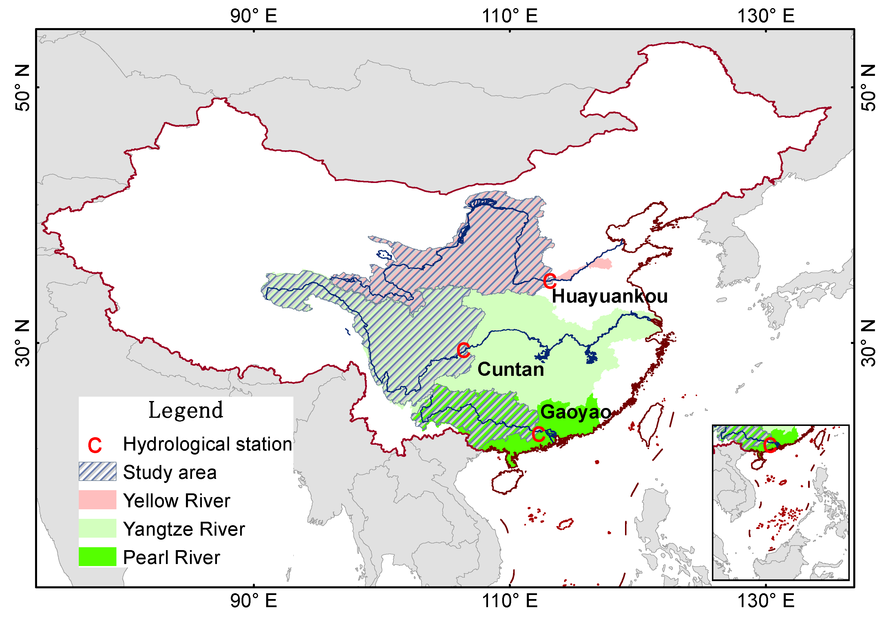
The Yellow River is the second largest river in China in terms of length and drainage area, and its basin covers a region of approximately 752,443 km2 (excluding an isolated inflow area of approximately 42,000 km2). Although accounting for approximately 2% of China’s national water resource, it irrigates 15% of the cultivated area and supports 12% of the population [19]. The river has been and will continue to be threatened by the effects of severe water scarcity [3]. Most areas of the basin are subject to semiarid or arid climatic conditions. During 1961–2019, the areal annual mean temperature and precipitation varied in the range of 8.1–10.5 °C and 341–703 mm, respectively. Precipitation during the summer flood period (June–September) accounts for approximately 68% of the annual total. However, the observed runoff during this period accounts for 48% of the annual total due to the effects of the climate and human activities, especially reservoir regulation. This study focused on the watershed located upstream of the Huayuankou hydrological station, which marks the division between the middle and lower reaches of the Yellow River (Figure 1). The area of the studied watershed accounts for 97% of the entire area of the Yellow River Basin. Its natural discharge through the station generally accounts for more than 95% of the total runoff of the basin in the recent decade. However, it is influenced considerably by anthropogenic activities such as reservoir operation and diversion for irrigation.
2.1.2. Yangtze River
In terms of length and mean annual discharge, the Yangtze River is the largest river in China and the third largest river in the world. It covers an area of approximately 1.8 million km2 and supports a population of over 440 million people [1]. The water resource of the basin (approximately 975.5 billion m3) accounts for 36% of the national river runoff. It supports more than 40% of China’s population and gross domestic product (GDP). Its tributaries belong to high-cold, subtropical, and temperate climatic zones. During 1961–2019, the areal annual mean temperature and precipitation varied in the range of 15.1–16.8 °C and 964–1411 mm, respectively. Annual precipitation in the basin varies from 324 to 500 mm in northwestern regions to 1600–2618 mm in southeastern parts. In addition, 80% of the annual precipitation falls during the rainy season (April–October) and approximately 43% of the annual precipitation falls in summer (June–August). The spatiotemporal variation of precipitation often leads to drought/flood hazards. This study focused on the upper reaches located upstream of the Cuntan hydrological station (Figure 1), which covers approximately 867,000 km2 and provides more than 80% of the river flow to the Three Gorges Project.
2.1.3. Pearl River
The Pearl River is the third largest river in China in terms of length and the second largest in terms of mean annual discharge. Its drainage basin covers an area of approximately 453,700 km2. Its water resources, which account for approximately 16% of China’s national total [20], are used to irrigate approximately 3% of the national cropland and to support 14% of the national population [21]. This study focused on the Xijiang River, which is the largest tributary of the Pearl River. It extends for 2214 km and drains western and central parts of the Pearl River Basin, accounting for 78% of the total area of the Pearl River Basin. The watershed area upstream of its outlet hydrological station (Gaoyao station) accounts for 99% of the area of the Xijiang River Basin. The locations of the Xijiang River Basin and the Gaoyao hydrological station are shown in Figure 1. During 1961–2019, the areal annual mean temperature and precipitation varied in the range of 18.7–20.4 °C and 1071–1786 mm, respectively. Dominated by the East Asian summer monsoon, 78% of the annual precipitation falls during the flood season (April–September) when runoff accounts for 74% of the annual total [3].
2.2. Climate Date
The observed daily precipitation and mean air temperature from 1958 to 2018, obtained from the National Meteorological Information Center of the China Meteorological Administration, were used to calibrate and validate the hydrological model, and then used to generate a reference run and to provide ICs for the hydrological hindcasts as meteorological forcings.
Meteorological hindcasts were derived from BCC_CSM1.1m, which is an operational seasonal forecast system of the Beijing Climate Center of the China Meteorological Administration. Its atmospheric circulation component model is a spectral model with about 100 km horizontal resolution (~1.0° × 1.0°) at the middle latitude region and 26 vertical levels [18], which has operated monthly since January 2016. It produces 13-month climate forecasts for 24 ensemble members using a lagged average forecasting strategy with 6-h intervals of atmospheric ICs of the final 6 days in a month. As CGCMs inevitably have biases and their spatial resolutions are usually too coarse for hydrological applications [22], monthly hindcasts are obtained only if the forecasting period exceeds 2 months. Therefore, anomaly bias correction and temporal disaggregation were applied to obtain the daily forcing at each grid of the hydrological hindcasts during 1991–2018.
2.3. Calibration and Validation of Hydrological Model and Streamflow Date
There are various versions of the HBV hydrological model. The original semi-distributed conceptual hydrological model HBV was developed by the Swedish Meteorological and Hydrological Institute [23]. In this study, a derivative of the “Nordic” HBV model, HBV-D was used to simulate streamflow. It is a semi-distributed basin-scale hydrological model, which divides a basin into small hydrological units, and can simulate the daily river flow and water balance. Compared to the original HBV, HBV-D results in an improved description of land cover characteristics and more physically sound evapotranspiration schemes [24]. The model was ever calibrated for the upper reaches of the Yangtze River [6], the Yellow River, and the Xijiang River [3] using the observed discharge and simulated discharge forced by gridded re-analysis climate data. To reduce the uncertainty associated with both hydrological parameterization and climate forcing, calibration and validation of the hydrological model were repeated for the three studied basins using climate observations other than the gridded re-analysis forcing as in previous studies, as well as the longest available records of streamflow data. Information on the naturalized monthly streamflow through the Huayuankou hydrological station during 1961–1998, observed streamflow through the Gaoyao station during 1960–2006, and observed streamflow through the Cuntan station during 1961–2006 was available and used.
The performance of HBV-D for the three river basins was evaluated using the following indices: Nash—Sutcliffe efficiency (NSE), coefficient of determination (R2), and percent bias (Pbias). They were calculated using Equations (1)–(3), respectively. An NSE efficiency of 1 corresponds to a perfect match of simulated discharge to the observed data. An efficiency of 0 (NSE = 0) indicates that the model simulations are as accurate as the mean of the observed data, whereas an efficiency less than 0 (NSE < 0) occurs when simulation is worse than the observed mean. The value of R2 indicates the relationship between observation and simulation. The greater R2 is, the higher the correlation is. Pbias can help identify the average model simulation bias (over simulation vs. under simulation). In accordance with the recommendation by Moriasi et al. (2015) [25], the performance of a watershed-scale model can be judged “satisfactory” for flow simulations if the following criteria are met: Monthly R2 > 0.60, NSE > 0.50, and |Pbias| < 15%. Furthermore, the monthly discharge simulation was also compared with observations using matched curves of month-to-month sequencing.
where is the observed discharge for the record, i, is the observed mean of all the observed discharge, is the simulated discharge for record i driven by the observed climate, and is the mean of all the simulated discharge.
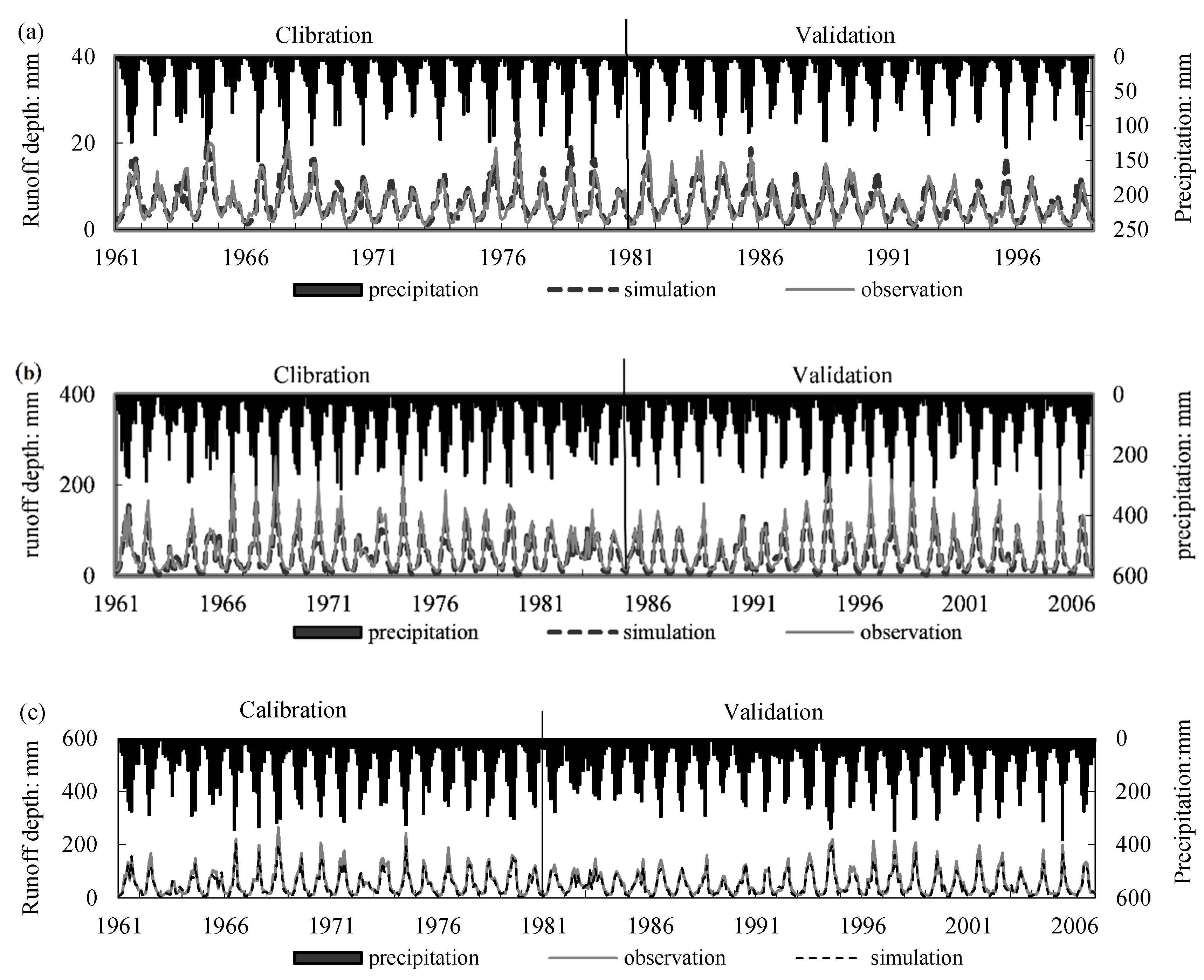
As listed in Table 1, the values of both NSE and R2 were >0.7 and the value of |Pbias| was <15% during the calibration and validation periods for the three basins, i.e., within the “satisfactory” range. Moreover, the monthly simulations matched the observations well, as shown in Figure 2. Therefore, the performance was judged satisfactory and the model was considered highly suitable for application to the three basins. Then, as in most previous related research, the calibrated HBV model was used to simulate streamflow without consideration of human interventions such as reservoir management.
2.4. Assessment of Hydrological Hindcast Skill
2.4.1. Skill Metrics
The performance of the hydrological hindcasts was determined using pseudo observations for 1991–2018, based on the simulation forced by the observed climate. The anomaly percentage of streamflow other than streamflow was applied since anomaly forecasting is more important and more skillful than that of the streamflow itself.
The skill of deterministic streamflow forecasting was measured in terms of the anomaly correlation coefficient (ACC), which was used to measure the phase errors. A forecast can be considered perfect for a case with ACC = 1, whereas it is determined worse than the reference situation for a case with ACC < 0. Correlation is considered significant at the 0.05 significance level for a case with ACC > 0.367.
Another performance metric, i.e., the relative operating characteristics (ROC) area, was used to measure the skill of probabilistic forecasting. The areas of ROC_A, ROC_N, and ROC_B represent the three categories of above normal, near normal, and below normal, respectively. A forecast can be considered to have a certain skill for a case where the ROC area is >0.5, whereas it has no valid information for a case where the ROC area is ≤0.5. All metrics were measured at a monthly resolution rather than a seasonal resolution.
For convenience and ease in the investigation of the tendency of skill with the extension of lead time and the relationship between skill metrics and between rivers, the mean skill score at the level of the lead time was calculated using Equation (4), and that of the mean overall lead time and target months was calculated using Equation (5) based on mathematical averaging:
where is the mean skill score at the level of lead time i (), is the skill score for lead time i and target month j (), and is the mean skill score over all lead times and target months.
2.4.2. Skill from Hydrological Initial Conditions and Meteorological Forcings
The skill of CGCM-based seasonal hydrological forecasting can usually be attributed to accurate hydrological ICs, advanced hydrological models, and accurately downscaled or bias-corrected CGCM precipitation and temperature [26]. To investigate the relative contributions to forecast skill from the hydrological ICs and MFs, conventional ESP and revESP have been widely used since the 1970s. One early application of ESP was the National Weather Service in the United States in the 1970s [27]. The theoretical framework of revESP was proposed and used to evaluate the importance of ICs and MFs by Wood and Lettenmaier (2008) [28]. Another two applications were Shukla and Lettenmaier (2011) [29], and Yuan et al. (2016) [19], where the roles of ICs and MFs were invested in the United States and in China, respectively. Usually, for the ESP method, a hydrological model with realistic ICs is driven by an ensemble of MFs resampled from the history. For the revESP, the hydrological model is driven by observed meteorological forcings with an ensemble of ICs from history.
In this study, for the ESP method, HBV-D with ICs of the target year was driven by an ensemble of MFs resampled from the history excluding the target year. For the revESP method, HBV-D is driven by the observed climate of the target year with an ensemble of ICs resampled from the history excluding the target year. ESP was used to isolate the skill attributable to the considered hydrological ICs, whereas revESP was used to separate the contributions of the MFs. The relative importance of the hydrological ICs and MFs in streamflow forecasting was measured based on the RMSE ratio (RMSEESP/RMSErevESP). The importance of the hydrological ICs was considered to outweigh that of the MFs for the target month if the variance ratio was <1. Conversely, the MFs were considered to prevail over the ICs if the ratio was >1.
2.4.3. Experimental Design
Four experimental schemes were designed to assess the performance of the proposed seasonal streamflow forecasting system, and to measure the relative importance of the ICs and MFs in streamflow forecasting.
- (1)
- Ref-sim: A continuous simulation from 1991 to 2018 driven by the observed climate was used to generate the hydrological ICs at the beginning of each calendar month, the reference streamflow, and soil moisture for the assessment of the naturalized hydrological predictability over the three basins.
- (2)
- ESP-sim: ESP simulations initialized at the beginning of each calendar month during 1991–2018, with annually varying hydrological ICs identical to experiment (1) and with 27 realizations of 7-month MFs taken from the same period of the target year while excluding the target year. For example, for an ESP simulation starting in February 1991, the ICs were identical to experiment (1) in January 1991, and the 27 ensembles of the MFs were those in experiment (1) during February–July of 1992–2018 but without using the MFs in the target year (i.e., 1991).
- (3)
- RevESP-sim: The revESP simulations were generated with annually varying MFs identical to experiment (1) but with 27 ensembles of hydrological ICs taken from different years excluding the target year. For example, for the revESP simulation starting in January 1991, the MFs were those in experiment (1) during February–July of 1991, while the 27 ensembles of ICs were taken from January of 1992–2018 but without using the ICs in January of the target year (i.e., 1991).
- (4)
- Full-hind: Full hindcasting simulations were generated with annually varying hydrological ICs taken from the same date of experiment (1) and with 24 ensembles of MFs from CSM_1.1m for the 6 target months. For example, for the full hindcasting simulation starting in February 1991, the ICs were identical to experiment (1) in January 1991, while the MFs were the 24 ensemble hindcasts from CSM_1.1m during February–July of 1991.
3. Results
3.1. Yellow River
3.1.1. Skill of Deterministic Streamflow Hindcasts
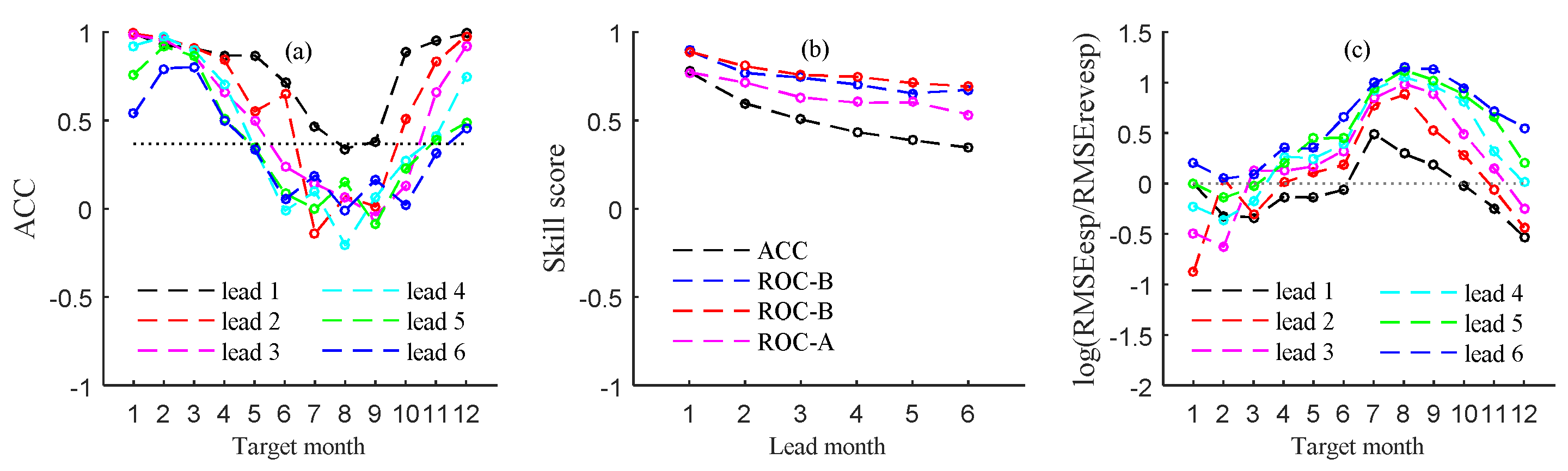
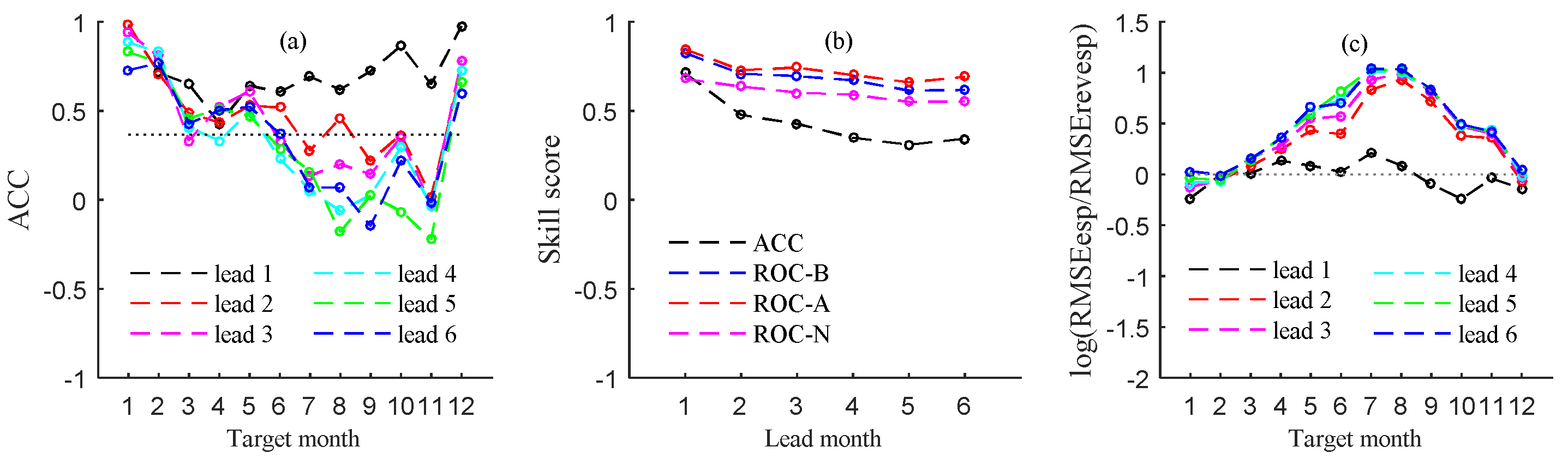
The seasonal variation of the ACC for the six lead times for the Yellow River is shown in Figure 3a. It can be seen that there is a decreasing (increasing) tendency before (after) summer. Therefore, the ACC is generally smaller for target months in summer than in other seasons. However, the ACC is significant at the 0.05 significance level for almost all target months for lead month 1, and it is significant for those months during winter and the first 2 months of spring (i.e., December–April) for the other five lead times. This suggests that streamflow forecasting with the proposed method is generally skillful for most target months for lead month 1, and that it is more skillful for dry and relatively drier months during transition seasons than for other months for all six lead times. It can also be observed in Figure 3b that there is a tendency of decline with the extension of lead time, i.e., the ACC of 0.774 for lead month 1 decreases to 0.346 for lead month 6. A similar decreasing tendency can also be seen in Figure 3a, where the ACC is significant for 11 target months for lead time 1 but for only 5 target months for lead month 6.
3.1.2. Skill of Probabilistic Streamflow Hindcasts
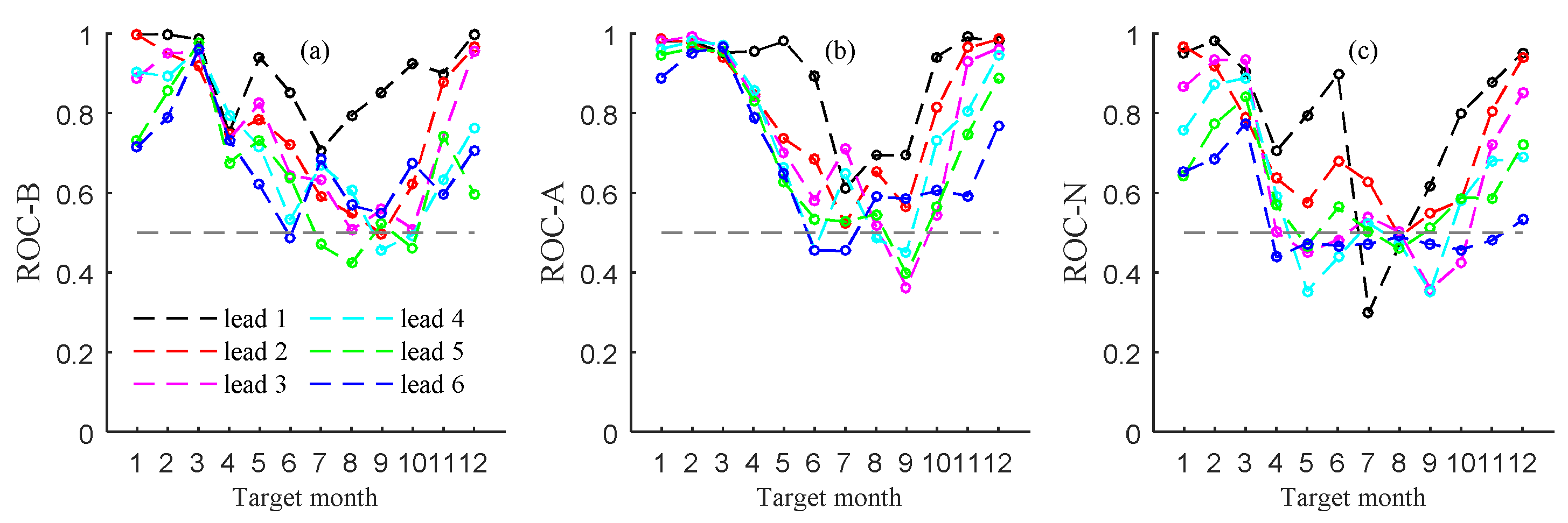
The seasonal variation of the ROC areas for three tercile categories for the six lead times for the Yellow River is illustrated in Figure 4. The ROC areas for the below-normal tercile are >0.5 for target months during winter, spring, and the final month of the transition from wet to dry seasons (i.e., November–May) for all six lead times, and even for all 12 months for lead month 1, but <0.5 for most target months during the summer flood season for lead months 5 and 6 (Figure 4a). A similar seasonal variation in the ROC areas for the above-normal tercile can be observed in Figure 4b, but the skillful target months extend forward to October from November for all six lead times, and even cover all 12 months for lead months 1 and 2. However, for the near-normal tercile, streamflow forecasting generally has no valid information for target months of April–November (Figure 4c). These findings reveal that skill is generally higher for target months during the dry season and certain months during the transition season than for wet months, higher for the abnormal terciles than for the near-normal tercile, and higher for the above-normal tercile than for the below-normal tercile. The ROC area is 0.738, 0.642, and 0.767 for the below-normal, near-normal, and above-normal terciles, respectively, over all target months and all six lead times (Table 2), suggesting that skill is highest (lowest) for the forecasting of the above-normal (normal) tercile. The relationship between the three categories illustrates a tendency of decline of the ACC with the extension of lead time (Figure 3b).
3.1.3. Streamflow Predictability from Hydrological ICs and MFs
The seasonal variation of the ratio of the RMSE of streamflow from the ESP simulations to that from the revESP simulations is shown in Figure 3c. All the ratio curves show peaked shapes that indicate that the greatest values are associated with the wet season. However, the values of <1.0 are concentrated in target months of October–June for lead month 1, of November–March for lead month 2, of December–February for lead month 3, and of January–March for lead months 4 and 5. There are no target months with values of <1.0 for lead month 6. These findings suggest that hydrological ICs play a dominant role in the dry season and the relatively drier months of the transition seasons, but that the importance of this role declines as the lead time increases. The duration of influence of the ICs is up to 3 months in the dry season and early spring, but it is only 1 month in mid–late spring and early summer. The MFs play a dominant role for target months of July–September (May–October) from the 1st (3rd) month forecast.
3.2. Yangtze River
3.2.1. Skill of Deterministic Streamflow Hindcasts
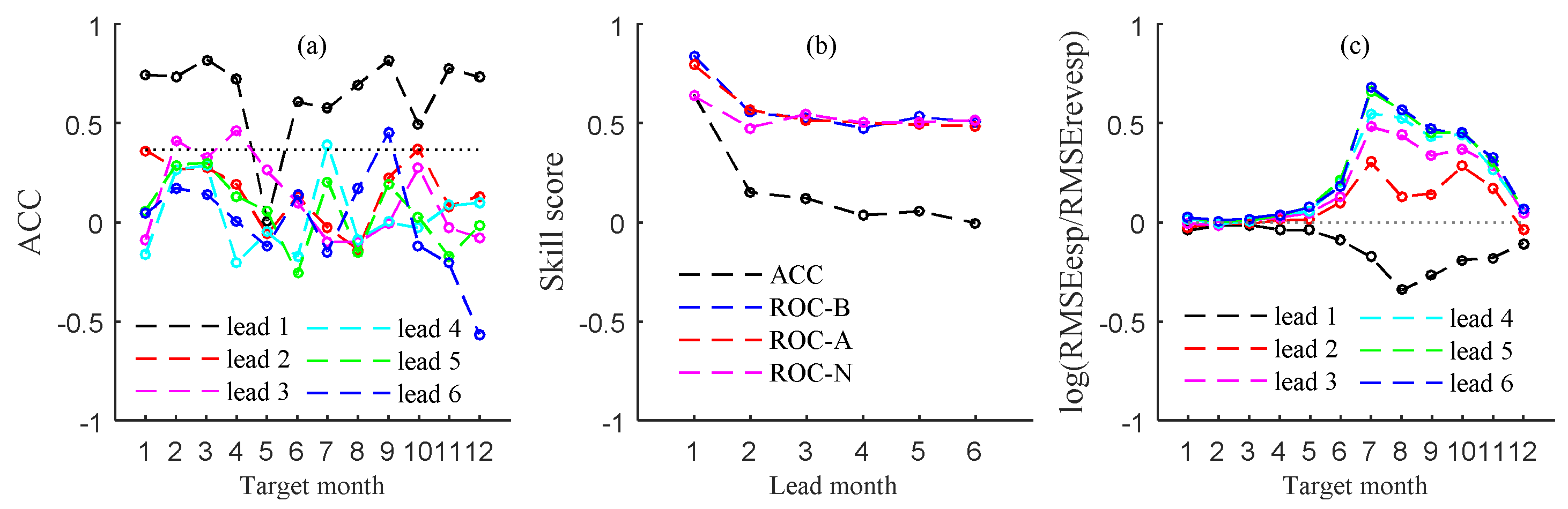
The seasonal variation of the ACC for the Yangtze River, illustrated in Figure 5a, shows that the ACC is significant for all 12 target months for lead month 1 at the 0.05 significant level, for December–June for lead month 2, and generally significant for December–May for lead months 3–6. These findings suggest that streamflow forecasting is generally more skillful for winter and spring than for other seasons, and that it is more skillful for a shorter lead time than for a longer lead time. The ACC curves at the lead time level further illustrate the tendency of decline with the extension of lead time (Figure 5b). The greatest (smallest) value of the ACC is 0.711 (0.309) for lead month 1 (5).
3.2.2. Skill of Probabilistic Streamflow Hindcasts
The ROC areas for the two abnormal terciles show a decreasing tendency during the earlier months and an increasing tendency during the following months with different turning points for different lead times (Figure 6a,b). The ROC areas are >0.5 for all target months for lead months 1–3 for the below terciles, and for more than 8 target months, including those in winter, spring, and some of the other seasons, for lead months 4–6. In comparison with the below-normal tercile, the skillful periods for the above-normal tercile are slightly extended. Among the skillful target months, the ROC areas are generally higher for those in winter and spring than in other seasons. Similar to the abnormal terciles, there are more skillful target months for the first three lead times than for the other three longer lead times, and the ROC areas for winter are relatively greater than in other seasons for all lead times except for lead month 6. However, there are slightly fewer skillful target months for the normal tercile than for the abnormal terciles. These findings suggest that skill is generally higher for shorter lead times than for longer lead times, higher for the dry season than for the wet season, and higher for the abnormal terciles than for the normal tercile. It can also be observed in Figure 5b that there is a tendency of decline with the extension of lead time and the relationship between the three tercile categories. The latter is presented more clearly in Table 2, where the mean ROC area is greatest (smallest) for the above-normal (normal) tercile. This further confirms that the streamflow forecasting skill is highest (lowest) for the above-normal (normal) tercile.
3.2.3. Streamflow Predictability from ICs and MFs
For the Yangtze River, it can be seen from Figure 5c that the ratio of the RMSE of streamflow from the ESP simulations to that from the revESP simulations is slightly smaller than 1.0 for the target months of December–February for lead months 2–5, and for the target months of September–February for lead month 1, although the ratio is close to 1.0 for February. For this wet river basin, these findings indicate that the slight dominance of the influence of the ICs usually persists for 5 months in winter but for only 1 month in autumn. However, the slight dominance of the influence of the MFs prevails in spring and summer for the first month forecast, but the role becomes more obvious from the second month forecast in these two seasons, as well as in autumn.
3.3. Xijiang River
3.3.1. Skill of Deterministic Streamflow Hindcasts
Different from the other two rivers, the curves of the seasonal variation of the ACC for the Xijiang River are more complex (Figure 7a). The ACC is significant for all target months other than May for lead month 1, and significant only for 1 or 2 target months for the other five lead times, suggesting that streamflow forecasting is skillful only for lead month 1. The tendency of decline with the extension of lead time is illustrated more clearly in Figure 7b, where the ACC is as high as 0.645 for lead month 1, but decreases abruptly to 0.152 for lead month 2 and falls to even smaller values for the longer lead times.
3.3.2. Skill of Probabilistic Streamflow Hindcasts
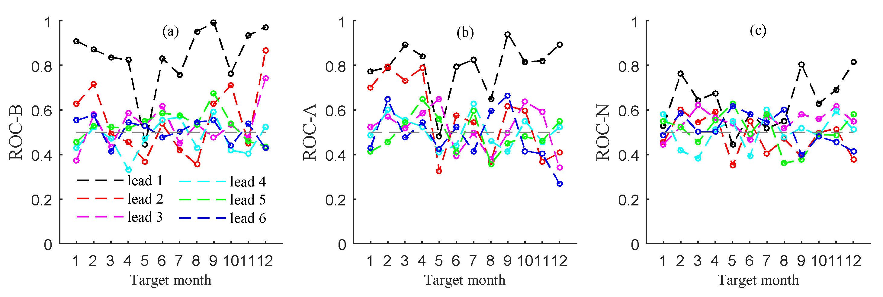
As shown in Figure 8, the changes of monthly ROC areas are complicated for the Xijiang River. They do not show a tendency with the delay of the target month but they are >0.5 for target months in winter. Similar to the other rivers, for the same target month, the ROC area is usually greater for lead month 1 than for other lead times and greater for the abnormal terciles than for the normal tercile. The tendency of decline with the extension of lead time shown in Figure 7b is similar to that found for the other rivers. Overall, the mean ROC area is 0.573, 0.531, and 0.560 for the below-normal, near-normal, and above-normal terciles, respectively, over all target months and for all six lead times (Table 2).
3.3.3. Streamflow Predictability from ICs and MFs
The ratio of the RMSE of streamflow from the ESP simulations to that from the revESP simulations for the Xijiang River is shown in Figure 7c. It can be seen that the ratio is <1.0 for all 12 target months for lead month 1, but >1.0 for target months of June–November for the other five lead times, although the ratios are close to 1.0 for the first 5 months of the year. For this wet river basin, these findings indicate that the period over which the influence of the ICs is dominant is only 1 month in summer and autumn, and that the influence of the MFs prevails from the second month in both seasons. However, the importance of the role of the MFs is almost equal to that of the ICs in winter and spring.
3.4. Skill Comparison between Rivers
The values of the mean ACC and ROC areas for each river over all target months and lead months are listed in Table 2. The values are greatest (smallest) for the Yellow (Xijiang) River for any metric of skill, suggesting that streamflow forecasting is more skillful for dry rivers in northern China than for wet rivers in southern China.
4. Discussion and Conclusions
Based on the investigation of metrics of skill in terms of the ACC and ROC areas, and the relative influence of ICs and MFs in relation to the three studied rivers, certain findings related to streamflow predictability were revealed.
(1) There are more skillful target months and the skill scores are generally greater for lead month 1 than for longer lead times. This is consistent with the tendency of decline with the extension of lead month, which was highlighted by Greuell et al. (2018) [30] in relation to regions of Europe with snow-rich winters. This might be due to the low skill of climate models at local scales and to the declining influence of the ICs after the first month forecasts.
(2) As for seasonal variation of the skill metrics, the skill scores are generally higher for target months in winter and early spring than for those months during the wet period for the Yellow River, and generally higher for target months in winter than for those months in the wet period for the Yangtze River. However, no obvious seasonal variation was found for the Xijiang River. This suggests that streamflow prediction is more skillful for potential drought forecasting than for flood forecasting in the Yellow and Yangtze rivers.
(3) Generally, in terms of both the ACC and the ROC area, streamflow forecasting is more skillful for the dry river in northern China than for the two wet river basins in southern China. Moreover, forecasting is more skillful for the abnormal terciles than for the near-normal tercile for each of the three rivers, more skillful for the above-normal tercile than for the below-normal tercile for the Yellow and Yangtze rivers, and more skillful for the below-normal tercile than for the above-normal tercile for the Xijiang River.
(4) The period of dominance of the influence of the hydrological ICs and MFs depends on the season and geographic location. The prevailing role of the ICs is concentrated in the dry season for the Yellow River, during which the period of dominance of the influence of the ICs can persist for up to 5 months. Although the period and duration of the influence of the ICs are largely the same as for the Yellow River, the influence of the ICs declines for the Yangtze River. Different from the other two rivers, the period of dominance of the influence of the ICs for the Xijiang River is concentrated in the first month of summer and autumn and the influence prevails for only 1 month. From the second month forecast, the MFs play an obvious prevailing role in the wet season and the relatively wetter periods of the transition seasons for all the three rivers. Similar findings were revealed by both Yuan et al. (2016) [19] and Wood and Lettenmaier (2008) [28], where the importance of the MFs was found to outweigh that of the ICs during the wet season, and the duration of the influence of the ICs varied from 2 to 5 months during the dry season for the Yellow River Basin, and where the ICs yielded the streamflow forecasting skill for up to 5 months during the transition period between the wet and dry seasons in northern California (USA). The differences in the seasons and durations of influence of the ICs between the above studies could possibly be attributed to uncertainties associated with the hydrological modeling, MF datasets, and river locations.
(5) Target months in winter with higher skill scores match well with periods when the influence of the ICs outweighs that of the MFs, and target months in wet periods with lower skill scores generally match with periods when the influence of the MFs outweighs that of the ICs for the Yellow and Yangtze Rivers. These findings suggest dominance of the influence of the ICs (MFs) on streamflow predictability in the dry (wet) season and for dry (wet) rivers. To improve the streamflow forecasting skill in the dry season and for dry rivers, it is more important to obtain precise hydrological conditions. However, in the wet season and for wet rivers, the streamflow forecasting skill could be improved through various valid methods. For example, remote sensing information and streamflow assimilation by a hydrological model or a land surface model can improve the ICs (i.e., Montero et al. 2016 [31]; Mazrooei and Sankarasubramanian 2019 [32]), while bias-correcting outputs from CGCMs and multi-model ensemble predictions and dynamical downscaling can improve either the MFs or the ICs (i.e., Yuan et al. 2015 [22]; Yao and Yuan 2018 [33]; Lee and Ahn 2019 [34]). In addition, the application of satellite and remote sensing products in hydrological model inputs [12,35], and hydrological postprocessing are able to increase the forecast skill and reduce uncertainty [15,22].
The findings of this study will help improve the understanding of the predictability of streamflow forecasting based on the output of a hydrological model driven by CSM. Moreover, the results reveal the focus for the improved streamflow forecasting skill, i.e., obtaining precise hydrological ICs in the dry season for dry rivers, and enhanced MFs in the wet season for wet rivers. However, a further investigation will be required to clarify the reasons for the complex seasonal variation of the skill metrics, elucidate the relative roles of the ICs and MFs (especially for the Xijiang River), and introduce various methods to improve hydrological forecasting. In addition, it is left for future work to investigate the uncertainty of skill of discharge predicted from the hydrological model structure.
Author Contributions
L.L. conceived and developed the design of the study, parameterized the HBV model for the Yellow and Xijiang Rivers, and was responsible for hydrological hindcasts, verification, and manuscript writing; J.Z. parameterized the HBV model for the Yangtze River; P.Z. contributed to the selection and explanation of the skill metrics. All authors (L.L., Y.W., P.Z., J.Z., L.Z. and C.X.) contributed to the interpretation of the results and improvement of the manuscript. All authors have read and agreed to the published version of the manuscript.
Funding
This research was funded by [National Key Research and Development Program of China; the Nonprofit Special Scientific Research supported by the China Meteorological Administration] grant number [2018YFE0196000 and 2017YFA0605004; GYHY201406021]. And the research was funded by the UK-China Research and Innovation Partnership Fund through the Met Office Climate Science for Service Partnership (CSSP) China as part of the Newton Fund.
Institutional Review Board Statement
Not applicable.
Informed Consent Statement
Not applicable.
Data Availability Statement
Data is contained within the article. They are also available on request from the corresponding author.
Acknowledgments
We greatly appreciate the editor and reviewers for their insightful comments and constructive suggestions that helped us to improve the manuscript. We also thank James Buxton for editing the English text of this manuscript.
Conflicts of Interest
The authors declare that they have no known competing financial interests or personal relationships that could have appeared to influence the work reported in this paper.
References
- Wang, Y.; Ding, Y.; Ye, B.; Liu, F.; Wang, J.; Wang, J. Contributions of climate and human activities to changes in runoff of the Yellow and Yangtze Rivers from 1950 to 2008. Sci. China Earth Sci. 2013, 56, 1398–1412. [Google Scholar] [CrossRef]
- Zhang, Q.; Zhang, Z.; Shi, P.; Singh, V.P.; Gu, X. Evaluation of ecological instream flow considering hydrological alterations in the Yellow River basin, China. Glob. Planet. Chang. 2018, 160, 61–74. [Google Scholar] [CrossRef]
- Liu, L.; Jiang, T.; Xu, H.M.; Wang, Y. Potential threats from variations of hydrological parameters to the Yellow River and Pearl River Basins in China over the Next 30 Years. Water 2018, 10, 883. [Google Scholar] [CrossRef] [Green Version]
- Gemmer, M.; Jiang, T.; Su, B.; Kundzewicz, Z.W. Seasonal precipitation changes in the wet season and their influence on flood/drought hazards in the Yangtze River Basin, China. Quat. Int. 2008, 186, 12–21. [Google Scholar] [CrossRef]
- Wang, Y.; Liao, W.; Ding, Y.; Wang, X.; Jiang, Y.; Song, X.; Lei, X. Water resource spatiotemporal pattern evaluation of the upstream Yangtze River corresponding to climate changes. Quat. Int. 2015, 380–381, 187–196. [Google Scholar] [CrossRef]
- Su, B.; Huang, J.; Zeng, X.; Gao, C.; Jiang, T. Impacts of climate change on streamflow in the upper Yangtze River basin. Clim. Chang. 2017, 141, 533–546. [Google Scholar] [CrossRef]
- Qin, P.; Xu, H.; Liu, M.; Du, L.; Xiao, C.; Liu, L.; Tarroja, B. Climate change impacts on Three Gorges Reservoir impoundment and hydropower generation. J. Hydrol. 2020, 580, 123922. [Google Scholar] [CrossRef]
- Gu, X.; Zhang, Q.; Liu, J.; Zhang, Z. Characteristics, causes and impacts of the changes of the flood frequency in the Pearl River drainage basin from 1951 to 2010. J. Lake Sci. 2014, 26, 661–670. (In Chinese) [Google Scholar]
- Yan, D.; Werners, S.E.; Ludwig, F.; Huang, H.Q. Hydrological response to climate change: The Pearl River, China under different RCP scenarios. J. Hydrol. Reg. Stud. 2015, 4, 228–245. [Google Scholar] [CrossRef] [Green Version]
- Cloke, H.L.; Pappenberger, F. Ensemble flood forecasting: A review. J. Hydrol. 2009, 375, 613–626. [Google Scholar] [CrossRef]
- Yang, L.; Tian, F.; Sun, Y.; Yuan, X.; Hu, H. Attribution of hydrologic forecast uncertainty within scalable forecast windows. Hydrol. Earth Syst. Sci. 2013, 10, 11795–11828. [Google Scholar] [CrossRef]
- Patil, A.; Ramsankaran, R. Improving streamflow simulations and forecasting performance of SWAT model by assimilating remotely sensed soil moisture observations. J. Hydrol. 2017, 555, 683–696. [Google Scholar] [CrossRef]
- Liang, Z.; Li, Y.; Hu, Y.; Li, B.; Wang, J. A data-driven SVR model for long-term runoff prediction and uncertainty analysis based on the Bayesian framework. Theor. Appl. Climatol. 2018, 133, 137–149. [Google Scholar] [CrossRef]
- Tongal, H.; Booij, M.J. Simulation and forecasting of streamflows using machine learning models coupled with base flow separation. J. Hydrol. 2018, 564, 266–282. [Google Scholar] [CrossRef]
- Yuan, X.; Wood, E.F. Downscaling precipitation or bias-correcting streamflow? Some implications for coupled general circulation model (CGCM)-based ensemble seasonal hydrologic forecast. Water Resour. Res. 2012, 48, 12519. [Google Scholar] [CrossRef]
- Liu, L.; Xiao, C.; Du, L.; Zhang, P.; Wang, G. Extended-range runoff forecasting using a one-way coupled climate–hydrological model: Case studies of the Yiluo and Beijiang Rivers in China. Water 2019, 11, 1150. [Google Scholar] [CrossRef] [Green Version]
- Tan, Q.F.; Lei, X.H.; Wang, X.; Wang, H.; Wen, X.; Kang, A.Q. An adaptive middle and long-term runoff forecast model using EEMDANN hybrid approach. J. Hydrol. 2018, 567, 767–780. [Google Scholar] [CrossRef]
- Wu, T.; Song, L.; Li, W.; Wang, Z.; Zhang, H.; Xin, X.; Zhang, Y.; Zhang, L.; Li, J.; Wu, F.; et al. An overview of BCC climate system model development and application for climate change studies. J. Meteorol. Res. 2014, 28, 34–56. [Google Scholar] [CrossRef]
- Yuan, X.; Ma, F.; Wang, L.; Zheng, Z.; Ma, Z.; Ye, A.; Peng, S. An experimental seasonal hydrological forecasting system over the Yellow River basin—Part 1: Understanding the role of initial hydrological conditions. Hydrol. Earth Syst. Sci. 2016, 20, 2437–2451. [Google Scholar] [CrossRef] [Green Version]
- Pearl River Water Resources Commission of China. Pearl RiverWater Resources Bulletin. 2010. Available online: http://www.pearlwater.gov.cn/xxcx/szygg/10gb/ (accessed on 1 January 2017).
- Luo, L. The Drought Variation and Economic/Population Exposure in the Pear River Basin under the Climate Change. Mater Thesis, Chinese Academy of Meteorological Sciences, Beijing, China, 1999. [Google Scholar]
- Yuan, X.; Wood, E.F.; Ma, Z. A review on climate-model-based seasonal hydrologic forecasting: Physical understanding and system development. WIREs Water 2015, 2, 523–536. [Google Scholar] [CrossRef]
- Bergström, S. The HBV Model—Its Structure and Applications; Reports RH, No. 4; Swedish Meteorological and Hydrological Institute: Norrköping, Sweden, 1992.
- Krysanova, V.; Bronstert, A.; Müller-Wohlferl, D.I. Modelling river discharge for large drainage basins: From lumped to distributed approach. Hydrol. Sci. J. 1999, 44, 313–333. [Google Scholar] [CrossRef]
- Moriasi, D.N.; Gitau, M.W.; Pai, N.; Daggupati, P. Hydrologic and water quality models: Performance measure and evaluation criteria. Trans. Am. Soc. Agric. Biol. Eng. 2015, 58, 1763–1785. [Google Scholar]
- Yuan, X.; Wood, E.F.; Roundy, J.K.; Pan, M. CFSv2-based seasonal hydroclimatic forecasts over the conterminous United States. J. Clim. 2013, 26, 4828–4847. [Google Scholar] [CrossRef]
- Twedt, T.M.; Schaake, J.; Peck, F.L. National weather service extended streamflow prediction. In Proceedings of the 45th Western Snow Conference, Albuquerque, NM, USA, 18–21 April 1977; pp. 52–57. [Google Scholar]
- Wood, A.W.; Lettenmaier, D.P. An ensemble approach for attribution of hydrologic prediction uncertainty. Geophys. Res. Lett. 2008, 35, L14401. [Google Scholar] [CrossRef] [Green Version]
- Shukla, S.; Lettenmaier, D.P. Seasonal hydrologic prediction in the United States: Understanding the role of initial hydrologic conditions and seasonal climate forecast skill. Hydrol. Earth Syst. Sci. 2011, 15, 3529–3538. [Google Scholar] [CrossRef] [Green Version]
- Greuell, W.; Franssen, W.H.P.; Biemans, H.; Hujes, W.A. Seasonal streamflow forecasts for Europe—Part I: Hindcast verification with pseudo- and real observations. Hydrol. Earth Syst. Sci. 2018, 22, 3453–3472. [Google Scholar] [CrossRef] [Green Version]
- Montero, R.A.; Schwanenberg, D.; Krahe, P. Moving horizon estimation for assimilating H-SAF remote sensing data into the HBV hydrological model. Adv. Water Resour. 2016, 92, 248–257. [Google Scholar] [CrossRef]
- Mazrooei, A.; Sankarasubramanian, A. Improving monthly streamflow forecasts through assimilation of observed streamflow for rainfall-dominated basins across the CONUS. J. Hydrol. 2019, 575, 704–715. [Google Scholar] [CrossRef]
- Yao, M.; Yuan, X. Superensemble seasonal forecasting of soil moisture by NMME. Int. J. Climatol. 2018, 38, 2565–2574. [Google Scholar] [CrossRef]
- Lee, J.; Ahn, J.B. A new statistical correction strategy to improve long-term dynamical prediction. Int. J. Climatol. 2019, 39, 2173–2185. [Google Scholar] [CrossRef] [Green Version]
- Khaki, M.; Hoteit, I.; Kuhn, M.; Forootan, E.; Awange, J. Assessing data assimilation frameworks for using multi-mission satellite products in a hydrological context. Sci. Total Environ. 2019, 647, 1031–1043. [Google Scholar] [CrossRef] [PubMed] [Green Version]
Figure 1.
Locations of the study areas and hydrological stations.

Figure 2.
Observed and simulated monthly runoff during periods of calibration and validation at (a) Huayuankou station along the Yellow River, (b) Cuntan station along the Yangtze River, and (c) Gaoyao station along the Xijiang River.
Figure 2.
Observed and simulated monthly runoff during periods of calibration and validation at (a) Huayuankou station along the Yellow River, (b) Cuntan station along the Yangtze River, and (c) Gaoyao station along the Xijiang River.

Figure 3.
Variation of (a) anomaly correlation coefficient (ACC) and (c) ratio of forecast to the observation variance with the target month for six lead times, and (b) skill scores variation with the lead time in terms of ACC and relative operating characteristic (ROC) areas for the Yellow River.
Figure 3.
Variation of (a) anomaly correlation coefficient (ACC) and (c) ratio of forecast to the observation variance with the target month for six lead times, and (b) skill scores variation with the lead time in terms of ACC and relative operating characteristic (ROC) areas for the Yellow River.

Figure 4.
Variation of ROC areas for (a) below-normal, (b) above-normal, and (c) near-normal with the target month for six lead times for the Yellow River.
Figure 4.
Variation of ROC areas for (a) below-normal, (b) above-normal, and (c) near-normal with the target month for six lead times for the Yellow River.

Figure 5.
Variation of (a) ACC and (c) ratio of forecast to the observation variance with the target month for six lead times, and (b) skill scores variation with the lead time in terms of ACC and ROC areas for the Yangtze River.
Figure 5.
Variation of (a) ACC and (c) ratio of forecast to the observation variance with the target month for six lead times, and (b) skill scores variation with the lead time in terms of ACC and ROC areas for the Yangtze River.

Figure 6.
Variation of ROC areas for (a) below-normal, (b) above-normal, and (c) near-normal with the target month for six lead times for the Yangtze River.
Figure 6.
Variation of ROC areas for (a) below-normal, (b) above-normal, and (c) near-normal with the target month for six lead times for the Yangtze River.

Figure 7.
Variation of (a) ACC and (c) ratio of forecast to the observation variance with the target month for six lead times, and (b) skill scores variation with the lead time in terms of ACC and ROC areas for the Xijiang River.
Figure 7.
Variation of (a) ACC and (c) ratio of forecast to the observation variance with the target month for six lead times, and (b) skill scores variation with the lead time in terms of ACC and ROC areas for the Xijiang River.

Figure 8.
Variation of ROC areas for (a) below-normal, (b) above-normal, and (c) near-normal with the target month for six lead times for the Xijiang River.
Figure 8.
Variation of ROC areas for (a) below-normal, (b) above-normal, and (c) near-normal with the target month for six lead times for the Xijiang River.


Table 1.
Performance of hydrologiska byråns vattenbalansavdelning (HBV) simulations for the monthly streamflow in the study areas.
Table 1.
Performance of hydrologiska byråns vattenbalansavdelning (HBV) simulations for the monthly streamflow in the study areas.
| Basin | Hydrological Station | Calibration | Validation | ||||
|---|---|---|---|---|---|---|---|
| NSE | R2 | Pbias | NSE | R2 | Pbias | ||
| Yellow River | Huayuankou | 0.76 | 0.77 | 3.7% | 0.73 | 0.74 | 3.7% |
| Yangtze River | Cuntan | 0.86 | 0.86 | −0.9% | 0.71 | 0.74 | 9.8% |
| Xijiang River | Gaoyao | 0.94 | 0.96 | −9.5% | 0.93 | 0.94 | −12.5% |
Table 2.
Mean skill metrics over all target months and lead times for the study areas.
| Basin | ACC | Below-Normal | Near-Normal | Above-Normal |
|---|---|---|---|---|
| Yellow River | 0.507 | 0.738 | 0.642 | 0.767 |
| Yangtze River | 0.436 | 0.688 | 0.601 | 0.728 |
| Xijiang River | 0.168 | 0.573 | 0.531 | 0.560 |
Publisher’s Note: MDPI stays neutral with regard to jurisdictional claims in published maps and institutional affiliations. |
© 2021 by the authors. Licensee MDPI, Basel, Switzerland. This article is an open access article distributed under the terms and conditions of the Creative Commons Attribution (CC BY) license (http://creativecommons.org/licenses/by/4.0/).
Share and Cite
MDPI and ACS Style
Liu, L.; Wu, Y.; Zhang, P.; Zhai, J.; Zhang, L.; Xiao, C. Predictability of Seasonal Streamflow Forecasting Based on CSM: Case Studies of Top Three Largest Rivers in China. Water 2021, 13, 162. https://doi.org/10.3390/w13020162
AMA Style
Liu L, Wu Y, Zhang P, Zhai J, Zhang L, Xiao C. Predictability of Seasonal Streamflow Forecasting Based on CSM: Case Studies of Top Three Largest Rivers in China. Water. 2021; 13(2):162. https://doi.org/10.3390/w13020162
Chicago/Turabian StyleLiu, Lyuliu, Ying Wu, Peiqun Zhang, Jianqing Zhai, Li Zhang, and Chan Xiao. 2021. "Predictability of Seasonal Streamflow Forecasting Based on CSM: Case Studies of Top Three Largest Rivers in China" Water 13, no. 2: 162. https://doi.org/10.3390/w13020162
Note that from the first issue of 2016, this journal uses article numbers instead of page numbers. See further details here.