Transport of Gaseous Hydrogen Peroxide and Ozone into Bulk Water vs. Electrosprayed Aerosol


Division of Environmental Physics, Faculty of Mathematics, Physics and Informatics, Comenius University, Mlynská Dolina, 842 48 Bratislava, Slovakia
*
Authors to whom correspondence should be addressed.
Water 2021, 13(2), 182; https://doi.org/10.3390/w13020182
Submission received: 30 November 2020
/
Revised: 8 January 2021
/
Accepted: 10 January 2021
/
Published: 14 January 2021
(This article belongs to the Special Issue Applications of Plasma Activated Water and Media in Medicine and Agriculture)
Abstract
:Production and transport of reactive species through plasma–liquid interactions play a significant role in multiple applications in biomedicine, environment, and agriculture. Experimental investigations of the transport mechanisms of typical air plasma species: hydrogen peroxide (H2O2) and ozone (O3) into water are presented. Solvation of gaseous H2O2 and O3 from an airflow into water bulk vs. electrosprayed microdroplets was measured, while changing the water flow rate and applied voltage, during different treatment times and gas flow rates. The solvation rate of H2O2 and O3 increased with the treatment time and the gas–liquid interface area. The total surface area of the electrosprayed microdroplets was larger than that of the bulk, but their lifetime was much shorter. We estimated that only microdroplets with diameters below ~40 µm could achieve the saturation by O3 during their lifetime, while the saturation by H2O2 was unreachable due to its depletion from air. In addition to the short-lived flying microdroplets, the longer-lived bottom microdroplets substantially contributed to H2O2 and O3 solvation in water electrospray. This study contributes to a better understanding of the gaseous H2O2 and O3 transport into water and will lead to design optimization of the water spray and plasma-liquid interaction systems.
1. Introduction
Interactions of non-equilibrium plasmas with liquids, known as plasma–liquid interactions [1,2,3], have become an emerging topic in the field of plasma science and technology, which contributed to many applications, ranging from environmental remediation [4,5] to material science [6], and health care [7,8]. The plasma interactions with liquids are of great importance in a plethora of various plasma–liquid systems because the liquid properties change in time under the interaction with plasma, and vice-versa [9]. The distinctive characteristics of non-equilibrium (cold) atmospheric plasmas, which are often created in ambient air, lead to a broad extension of their use in various biomedical applications [10,11,12,13,14,15]. Cold plasmas can be effective tools for microbial decontamination and sterilization [16], interact with living tissues [17], treat mammalian and cancerous cells [18], induce blood coagulation [16,19], can be applied in wound healing [20] and dentistry [21], and can be successfully transferred into clinical practice [14,15,22]. Novel applications in water cleaning, food production, and agriculture (e.g., seed germination and plant growth promotion, and pest control) without causing undesired side-effects or environmental burdens are on their way [23,24,25,26].
Atmospheric air plasmas in contact with liquid water or aqueous solutions generate “plasma-activated water” (PAW), which contains various reactive oxygen and nitrogen species (RONS), e.g., hydrogen peroxide (H2O2), nitrate (NO3−) and nitrite (NO2−) anions, ozone (O3), as well as other short-lived reactive species [23,27,28,29]. It has been reported by many research groups that these PAW solutions are effective in killing microbes and inactivating cancer cells [28,30,31,32]. PAW and other plasma-activated water solutions are examples of the outcome of plasma–liquid interactions, where the plasma RONS are transported/dissolved into water.
Species transport through the gas–liquid interface can be conceptualized by the change in density across the interface. This transition occurs over a few nanometers or less. The rough interface has fluctuations with water exchanging from the bulk to the boundary over several picoseconds [3]. Water considered as a model system in molecular dynamics simulations provided an atomic-level insight into the plasma–liquid film interaction mechanisms. It was found that plasma generated H2O2 species can travel through the water interface layer during 1.4 ns, penetrate deeper, and eventually reach the surface of biomolecules [33].
The plasma–liquid interface area is a key parameter maximizing the contact between the plasma and the treated water solution, thus determining the obtained plasma chemical effects [34]. Regarding typical long-lived plasma oxidizing species, H2O2, and its formation in multiple plasma–water systems has been extensively studied over the last decades. In a review by Locke et al., the formation of H2O2 was investigated in various plasma reactors with discharges directly in and over the liquid water with bubbles, and capillary discharges, in terms of H2O2 gas–liquid mass transfer characteristics. The highest H2O2 yields were found for the water droplet spray which provides large surface areas and small length scales to enhance the mass transfer rates [35]. Corona discharges yielded H2O2 production very similar to the other gas plasma reactors over water [36]. With a rising H2O2 amount in the gas phase, the aqueous H2O2 concentration increased whether H2O2 was created by the plasma in the gas phase or by the H2O2 bubbler (without plasma), with a slightly higher liquid H2O2 concentration for the plasma case [37]. Gaseous H2O2 produced near the air plasma–liquid water interface shows an extremely fast dissolution through this gas–liquid interface, as was demonstrated in the earlier study [31].
Transformation of bulk water into fine droplets or aerosol results in an increasing surface-to-volume ratio and thus accelerates the transport of RONS into the water, which is of vital importance for slowly soluble species, such as ozone. This concept has been adopted by several research groups [38,39,40,41], as well as our previous work [31,32,42]. For instance, in two different cold air plasma sources (streamer corona and transient spark discharge), PAW was prepared by the electrospray of fine aerosol droplets directly through the active plasma zone, which resulted in a very efficient transfer of gaseous RONS into water.
The enhanced transport of ozone into the water is of particular interest in the commercially used ozonation process that has become a common disinfection method for drinking water treatment due to its powerful oxidizing capacity and its ability to be applied at different stages throughout the treatment plant [43]. Mass transfer of ozone into the liquid water is considered one of the most important stages in the ozone oxidation technology to eliminate organic water contaminants [44]. The mass transport characteristics of O3 to the bulk water can be improved through non-porous membranes [45]. Wastewater treatment by ozone micro-nano-bubbles of sizes from tens of nanometers to tens of micrometers also leads to an enhancement of the surface-to-volume ratio, in a similar concept as by water aerosolization studied in this manuscript. The mass transfer efficiency of ozone to water was enhanced and controlled by the quantity and size of these ozone micro-nano-bubbles [46].
Electrospray (ES) or electrohydrodynamic atomization of liquids is one of the very efficient ways of producing liquid aerosols. It occurs from a conical meniscus located at the end of a capillary tube (nozzle) continuously supplied with liquid under the influence of a strong electric field. Positive and negative charges separate inside the liquid droplets, and charges of the same polarity as the nozzle, move towards the droplet surface, inducing a surface charge density on the liquid surface. The charged droplets generated from the nozzle of the high electric potential have different sizes ranging from large (mm) to very small (nm) droplets, at various droplet populations from polydisperse to monodisperse, at different flow rates, where the droplet diameter is controlled by varying the ES flow rate or the electrical conductivity of the liquid [47,48,49].
There are many parameters involved in the ES process, which determine different modes of continuous and intermittent ES, producing aerosols of highly varied characteristics. The key parameters are the geometry of the system used, the applied voltage, the dielectric strength of the ambient medium, the liquid flow rate, and the physical properties of the liquid, such as its electrical conductivity, surface tension, and viscosity. Due to the high electrical potential and low radii of the capillary nozzle, water meniscus, and the liquid jet at the nozzle outlet, the electric field is often sufficiently high to cause ionization processes in the surrounding gas. Corona discharge occurs at a low discharge power around the sharp edges of the nozzle where the electric field is locally applied [50]. The lifetime of the sub-micrometer liquid aerosol droplets (a few milliseconds) in cold atmospheric (corona) plasmas, is sufficient to produce many chemical reactions in the liquid aerosol [51].
Coupling of plasma–liquid interactions to the liquid ES with plasma-induced chemical processes has many technical advantages, as it employs the same device and the same high voltage power supply applied to the capillary nozzle. In addition, this configuration enables the efficient mass transfer of active species produced by plasma into the water droplets due to their micrometer-scale dimensions with a large surface-area-to-volume ratio [52]. The interest and applications of water ES for the liquid sprays have been applied to various areas due to their low cost, environment-friendly, and biocompatible water treatment [53].
Stancampiano et al. in their review conclude that plasma-aerosol droplets act as efficient microreactors where reaction rates, mixing and surface-to-volume ratio are enhanced. Ongoing experimental and simulation work in plasma control and precision microdroplet generation, as well as a better understanding of droplet transport for the in-situ delivery of chemicals, will lead to opening new horizons for future plasma–aerosol applications [54].
The novelty of the presented work is the experimental study of the transport mechanism of highly vs. weakly soluble cold air plasma generated reactive species into the water: namely H2O2 vs. O3. The transport of these species is compared separately, into the bulk water through a simple water surface, and into aerosols generated by the ES. H2O2 and O3 concentrations dissolved into the water are measured, and their depletion from the gas phase due to this transport. Changing the water flow rate and the applied voltage on the ES needle electrode is considered a turning point between the lower to the larger surface area of the produced water droplets. ES creates accelerated charged droplets with different sizes, average speeds, and lifetimes inside the reactor filled with the studied gaseous species. These parameters are controlled with various gas flow rates of gaseous H2O2 and O3 during different treatment times when the water (bulk or aerosol) is exposed to these incident H2O2 and O3 species. Experimental results coupled with theoretical calculations are presented and the solvation saturation coefficients for H2O2 and O3 are analyzed separately. These analyses will lead to a deeper understanding of the reactive gaseous plasma species transport (e.g., H2O2 and O3) into the water for various surface-to-volume ratios, which underlines ozonation and many air plasma applications in water cleaning and disinfection, biomedicine, and agriculture.
2. Theoretical Background
In general, the solubility of the gaseous species in liquids, e.g., water, is described by Henry’s law solubility coefficient :
where is the molar concentration of i-species in the aqueous phase and is the partial pressure of that species in the gas phase [55]. The is described as the proportionality factor of the amount of the dissolved gas in the aqueous phase to its partial pressure in the gas phase. In atmospheric chemistry, this coefficient is important to describe the distribution of trace species between the air and liquid droplets (aerosol). Henry’s law coefficient can be also expressed as the dimensionless ratio between the aqueous-phase concentration of a species and its gas-phase concentration in Equation (2), where and are the gas constant and temperature, respectively.
Henry’s law coefficient, however, does not describe the rate of the solvation process. It relates concentrations in the gas and the liquid phase in steady-state, with an equilibrated transfer (flux) of i-species from the gas into the liquid phase, and the backward transfer (flux) from the liquid into the gas phase. Out of equilibrium steady-state, which is typically the case in plasma–liquid interactions, these fluxes are not equal.
First, the flux of molecules from the gas into the liquid phase can be expressed:
Here, is the gas density of i-species, is their mean chaotic velocity, is their partial pressure, is the Boltzmann constant, and T is the gas temperature.
Next, the flux from the liquid phase back to the gas phase can be assumed proportional to the molar concentration of i-species in the liquid phase:
In the steady-state, these two fluxes are equal, and it is possible to derive the constant α using Henry’s law coefficient from Equation (1):
Knowing the fluxes in both directions, the number of transferred i-th molecules in time into the liquid phase with surface area, can be expressed as:
In combination with the expression , where is the volume of the liquid phase and is the Avogadro constant, an Equation describing the evolution of can be derived:
Assuming an initial concentration of i-species in the liquid phase to be zero, , this expression for the aqueous concentration of i-species at time is obtained,
It results from Equation (8) that with the increasing time, converges towards the steady-state (saturated) concentration. In this simplified theory, it was assumed that the partial pressure does not change in time and that the concentration in the liquid phase is homogeneous. The real situation is more complicated, but this formula demonstrates the importance of surface-to-volume ratio S/V and the role of . It is in qualitative agreement with computational modeling results obtained by Kruzselnicki et al. [56,57], who observed that for species with lower (e.g., O3), microdroplets are saturated quickly while for high species (e.g., H2O2), solvation continue to increase their aqueous densities longer. They also showed that the larger S/V ratio increases the rate of gas-phase solvation into the droplets if the droplet is under-saturated.
Hydrogen peroxide H2O2 and ozone O3 are examples of the plasma long-lived gaseous RONS. They have Henry’s law solubility coefficient , respectively. Henry’s law solubility coefficient of H2O2 is almost 7 orders of magnitude larger than that of O3. This means that while H2O2 readily transfers into the water through the gas–liquid interface, O3 is hardly dissolved into water based on its very low Henry’s law coefficient. For this reason, the assumption of constant partial pressure is generally valid only for low species (e.g., O3), as shown by Verlackt et al. [58], who investigated H2O2 and O3 as examples of highly and lowly soluble cold plasma species in a 2D axisymmetric fluid model. The density of H2O2 species shows a sudden drop at the gas–liquid interface due to the fast transfer into the liquid, where its density is significantly higher compared to the gas phase. On the other hand, the density of O3 species remains constant above the gas–liquid interface for 1 min of plasma treatment, where its density is much higher in the gas phase compared to the liquid phase.
For high species (e.g., H2O2), the gas density of species is not significantly depleted and can be considered constant only if the total volume of water is small and thus small amount of the gas phase species can be dissolved. Kruszelnicki et al. observed that for aerosol solvation, the H2O2 depletion is negligible only for microdroplets with a diameter below ~30 µm [57]. For bigger microdroplets with a larger volume, the surrounding H2O2 of these microdroplets was already depleted.
3. Materials and Methods
The transport of gaseous H2O2 and O3 generated by external sources into water is investigated in two types of reactors: bulk water and electrosprayed (ES) aerosols. The concentration of dissolved H2O2 and O3 in the water and their loss in the gas phase was measured. The optical imaging technique was employed to analyze the size, density, and surface area of the electrosprayed water microdroplets during the transport of H2O2 and O3 from air into water.
3.1. Generation and Analysis of H2O2 and O3 in the Gas Phase
Because of relatively low concentrations of H2O2 and O3 generated by the positive corona discharge that are typically used in biomedical applications [21,31,32,42], two different external gas sources of higher concentrations of H2O2 and O3 were used here. This enabled us to study the species transport into the water at higher gaseous concentrations. H2O2 and O3 gases were studied individually, where each one was mixed separately with an airflow to form a gas mixture with a specific dilution ratio, flow rate, and gas concentration. This gas mixture was pumped into two different reactors (ES and bulk) through PTFE tubes with an inner diameter of 4 mm and then measured by two individual electrochemical gas sensors of H2O2 and O3, type MEMBRAPOR. The gas sensors were connected to the reactor by PTFE and silicon tubes with the same inner diameter. Each gas sensor was attached to its transmitter board connected with an Arduino circuit, where the functional code is uploaded and displayed on LCD showing the gas concentrations in ppm.
The external source for H2O2 is a bubbler glass tube containing commercially available 30% (w/w) H2O2 solution in water with a corresponding molar concentration of 9.8 M. It is bubbled at room temperature using a variable airflow to produce H2O2 vapor with a high relative humidity >90%. This H2O2 vapor is mixed by a 1:1 ratio with dry air from an air pump to avoid the condensing of the water vapor in the H2O2 gas sensor and to keep the sensor’s recommended relative humidity range of 15–90%. The H2O2 gas sensor type H2O2/CB-500 has a nominal range of 0–500 ppm with a resolution <1 ppm and maximum overload of 1000 ppm. The H2O2 experiment was run at a concentration value of ~110 ppm of H2O2.
The O3 generator type EASELEC was used as an external source of O3 with an O3 output of 300 mg/h and a flow rate 2–3 L/min, which is mixed by 2:1 ratio with an airflow produced by an air pump to reach a stable concentration of ~450 ppm of O3 before starting the O3 experiment. Since the O3 generator has a constant output flow rate, a by-pass valve in one of its two output terminals was used to avoid limiting its designed gas flow rate and allow a lower concentration of O3 than its default output. The O3 gas sensor type O3/C-1000 has a nominal range of 0–1000 ppm with a resolution of 0.3 ppm and maximum overload of 2000 ppm.
The air-flow rate with H2O2 vapor or O3 gas was controlled using flow meters AALBORG. During each experiment of H2O2 or O3, the gas sensors are supposed to record a decrease in the H2O2 or O3 concentration of the gas mixture inside the reactor. This concentration loss in the gas phase represents how much of the H2O2 or O3 species were transported/dissolved into the water (bulk or aerosols).
3.2. Transport of Gaseous H2O2 and O3 into the Bulk Water
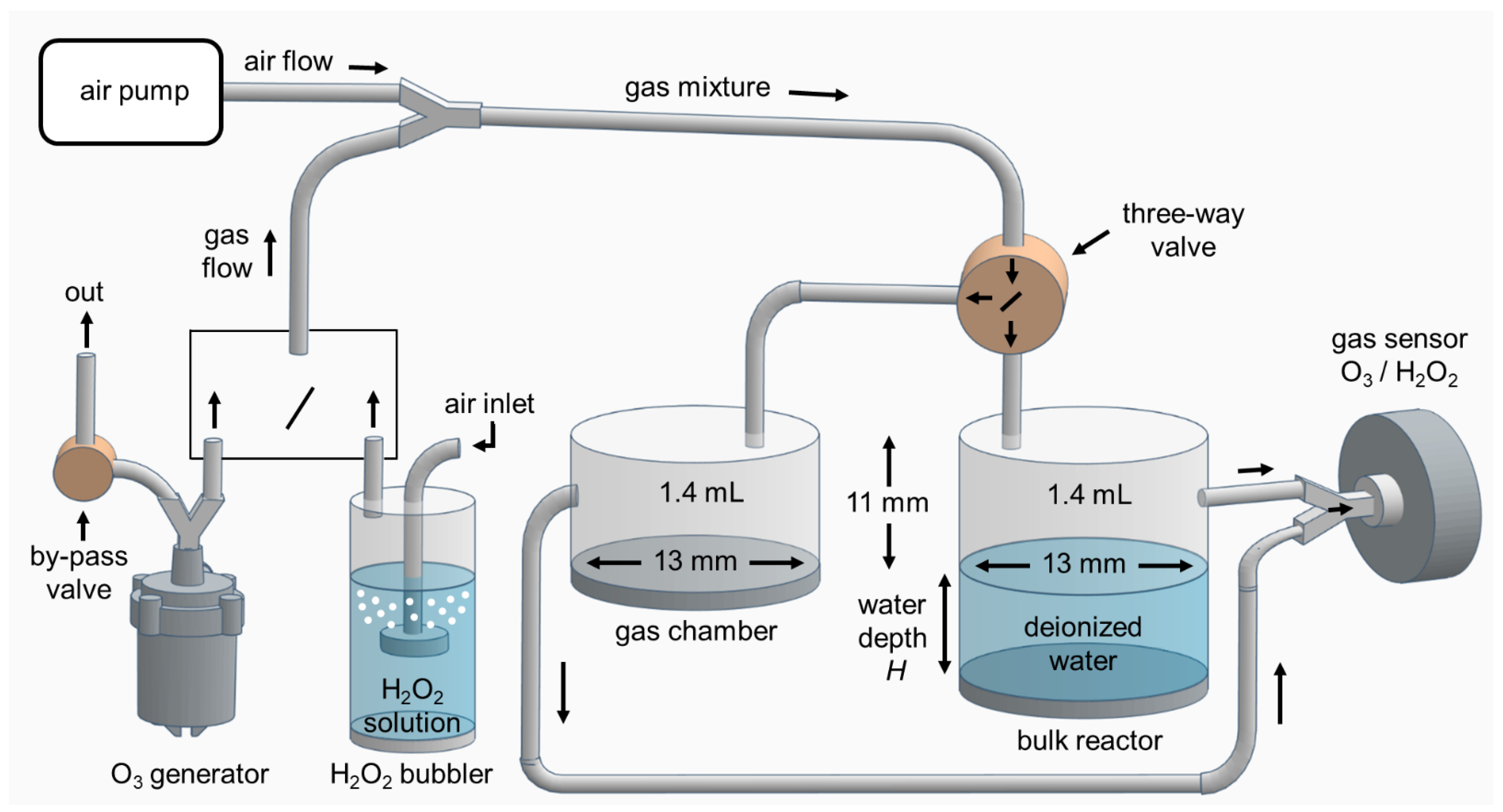
The experimental setup shown in Figure 1, consists of the air pump, external sources of H2O2 vapor and O3 gases, and gas sensors as described in the previous section.
The bulk water reactor and the gas chamber have the same cylindrical geometry and dimensions (diameter, height, and volume of the gaseous space 13 mm, 11 mm, and 1.4 mL, respectively) were used in parallel. There is a piston at the bottom of the bulk reactor to keep the height and volume of the gaseous space constant for different water volumes. The filled bulk of deionized water (with conductivity <3 µS/cm) at the bottom of the reactor has a fixed surface area exposed to H2O2 or O3 gaseous species. The volume of the bulk water is determined by its depth H.
The gas mixture of H2O2 diluted vapor or O3 diluted gas is first pumped through a three-way valve type BUERKLE PP/PE (Bad Bellingen, Germany) into the gas chamber with no water and then into the gas sensor. When reaching the stable starting point of the gas concentrations 110 or 450 ppm for the H2O2 vapor or O3 gas, respectively, the gas mixture is transferred into the bulk reactor filled with the specific water volume. At that moment, the treatment time is started, and the gas sensor is connected to the bulk reactor. The treatment time means the exposure time of this bulk water (with a fixed surface area and different volumes) to the incoming gas mixture. There was slight turbulence of the surface of the water bulk during the flow of the gas mixture at the highest flow rates used (2 L/min).
3.3. Analysis of the Sizes of Water Microdroplets using Fast/HS Camera Imaging and Transport of Gaseous H2O2 and O3 into the Water Aerosols
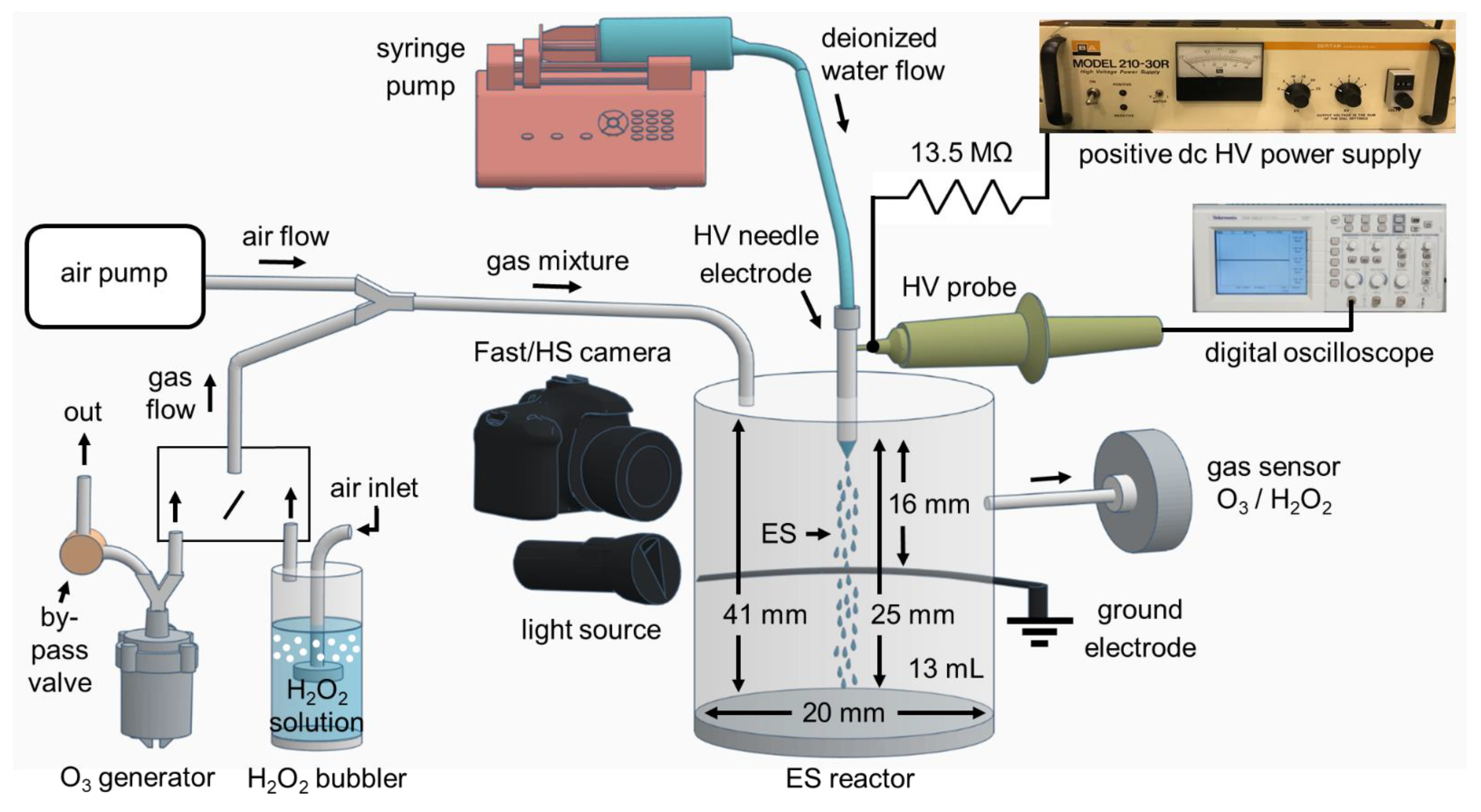
The diameter and density of the water aerosol (large droplets + electrosprayed microdroplets) were measured by high-speed visualization to investigate the transport of the gaseous species into the water. Figure 2 shows the schematic diagram of the ES experimental setup. It consists of a positive dc High Voltage (HV) power supply type Spellman’s Bertan model 210-30R of 135 W and a syringe pump type NE-300 which delivers the deionized water (with conductivity <3 µS/cm) continuously through a silicon tube with an inner diameter of 2 mm and controlled water flow rates (100–1000) µL/min into a blunt hollow needle electrode (anode) nozzle with the outer and inner diameters 0.7 and 0.5 mm, respectively. The needle electrode is placed opposite to a rounded wire of 1.5 mm diameter as a grounded electrode (cathode). The two electrodes are in point-to-plane geometry, both are stainless-steel with the shortest gap distance of 16 mm. HV from the power supply is applied through a ballast resistor 13.5 MΩ on the needle electrode. This HV is measured using a dc HV probe type AGILENT N2771A (Santa Clara, CA, USA) and then processed by a digital oscilloscope type TEKTRONIX TDS 1012 (Beaverton, OR, USA).
Two types of cameras placed in front of the water aerosols were used to visualize the electrosprayed aerosol and measure the size of the water droplets. A digital Fast camera type CASIO EXILIM was used mainly for the slower and larger size water droplets, with typical record parameters 60 fps (frame per second) and shutter speed 1/40,000 s (exposure time 25 µs). It provided photographs of the size 562 × 623 pixels and resolution 29.2 µm/pixel. Additionally, high speed (HS) camera Photron FASTCAM SA-Z type 2100K-C-32GB (Fujimi, Tokyo, Japan) was used mainly for the faster and lower size of the water microdroplets produced during the ES process, with typical record parameters 25,000 fps and shutter speed 1/50,000 s and 1/133,333 s (exposure time 20–7.5 µs) which provided photographs of the size 840 × 1024 pixels and resolution 21.875 µm/pixel.
To improve the spatial resolution of the camera at short exposure times and high shutter speed, sufficient light illumination was needed. The droplets were illuminated with two strong light sources, white LED type LEDLENSER P7R (Solingen, Germany) placed in front of the Fast camera with the droplets in between, and type DEDOLIGHT daylight 400D (Munchen, Germany) placed beside the HS camera directed to the microdroplets. The Fast/HS camera records photographs of the electrosprayed water microdroplets, which were processed and analyzed by the software Microsoft Office Picture Manager and GIMP (version 2.10.22).
To allow a very efficient mass transfer of the studied species (H2O2 and O3) into water aerosols and to enable the gas analyses and measurements, the HV needle and the ground wire electrodes were enclosed inside a transparent plastic reactor in which the water aerosols (large droplets + ES microdroplets) are produced and collected. It has a cylindrical geometry with the dimensions of diameter, height, and volume of gaseous space: 20 mm, 41 mm, and 13 mL, respectively. The transport process of H2O2 and O3 gaseous species into water aerosols occurs in this gaseous space along with a 25 mm flight distance of the water microdroplets from the needle electrode to the bottom of the reactor. The lifetime of these water microdroplets is the time before they reach the bottom of the ES reactor. There is an adjustable piston at the bottom of the reactor to keep the constant volume of the gaseous space and the flight distance when working with different water flow rates and treatment times.
Before starting the water flow and the applied HV on the needle electrode, the gas mixture of H2O2 vapor or O3 gas diluted with air was pumped into the ES reactor, and the gas sensors were employed for measuring their gas concentration. The H2O2 or O3 experiment started when the gas mixture concentration of H2O2 vapor or O3 gas reached 110 or 450 ppm, respectively. Then the water flow at the specific applied voltage on the needle electrode was started, for a given treatment time. The treatment time is the exposure time of the water aerosols to the gas mixture from the start until the end of the water flow.
3.4. Analysis of H2O2 and O3 in the Aqueous Phase Using UV-Vis Spectroscopy
The aqueous phase analysis is related to the amount of the gas concentrations of H2O2 and O3 in the gas phase, which are dissolved/transported into the water aerosols and bulk. UV-vis spectroscopy colorimetric methods were used for the chemical analysis of H2O2 and O3 in the aqueous phase. The collected water samples with added chemical reagents were analyzed by a UV/VIS absorption spectrophotometer UV-1800 Shimadzu.
For H2O2, TiOSO4 (titanium oxysulfate) reagent was used. H2O2 reacts with the titanium (IV) ions under acidic conditions which produced a yellow-colored product of pertitanic acid H2TiO4 with the absorption maximum at 407 nm [59]. The concentration of H2O2 is proportional to the absorbance according to Lambert–Beer’s law (molar extinction coefficient ε = 6.89 × 10² L/mol.cm).
For O3, a simple quantitative colorimetric standardized detection method was used for the dissolved O3 in water using the indigo blue reagent II for higher concentrations of O3 (0.05–0.5 mg/L) [32,60]. O3 decolorizes the indigo potassium trisulfonate dye rapidly in acidic conditions and the colorless product isatin is formed by the bleaching process. The decrease of the absorbance at 600 nm (ε = 2.38 × 10⁴ L/mol.cm) is linearly proportional to the increase of O3 concentration. Although this analytical method has limitations in air plasma-treated solutions due to cross-correlations with other plasma generated RONS, especially peroxynitrites [61], it can be safely used in this experiment with air containing O3 only.
4. Results and Discussion
The aim of the electrospray (ES) formation is to increase the size of the gas/plasma-liquid interface area compared to the bulk liquid experiments. In this section, the results from the bulk water solvation of O3 and H2O2 (Section 4.1) will be first presented and discussed, then the results of the visualization of microdroplets (Section 4.2). These experiments enabled us to estimate the surface area of electrosprayed microdroplets, which is then compared to the surface area in experiments with the bulk water. Measured molar amounts of dissolved O3 and H2O2 in the bulk experiment will be then compared to the results from ES solvation experiments (Section 4.3). Finally, a simple theoretical-analytical model will be presented to explain some of the observed phenomena (Section 4.4).
4.1. Solvation of O3 and H2O2 in Bulk Water
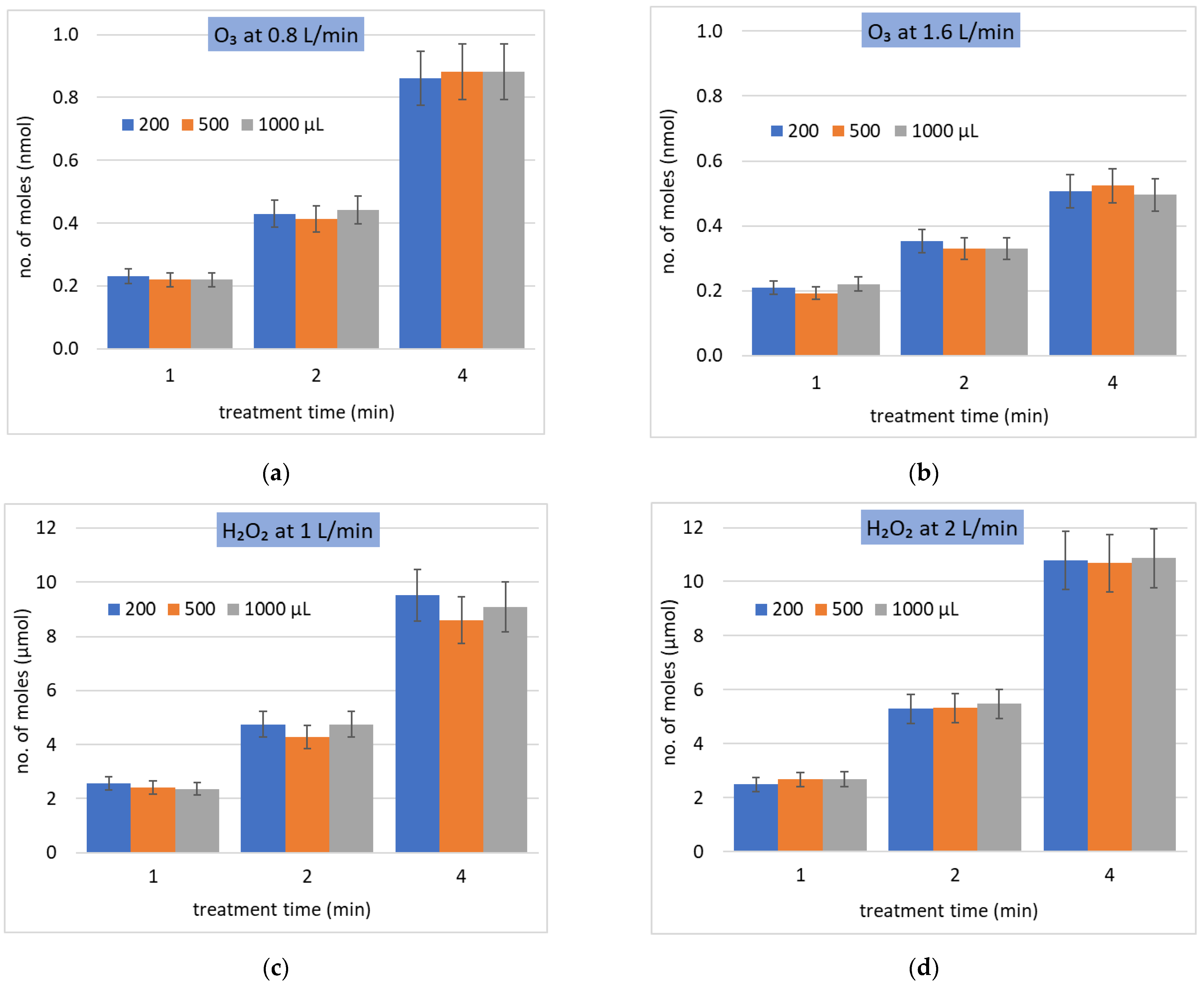
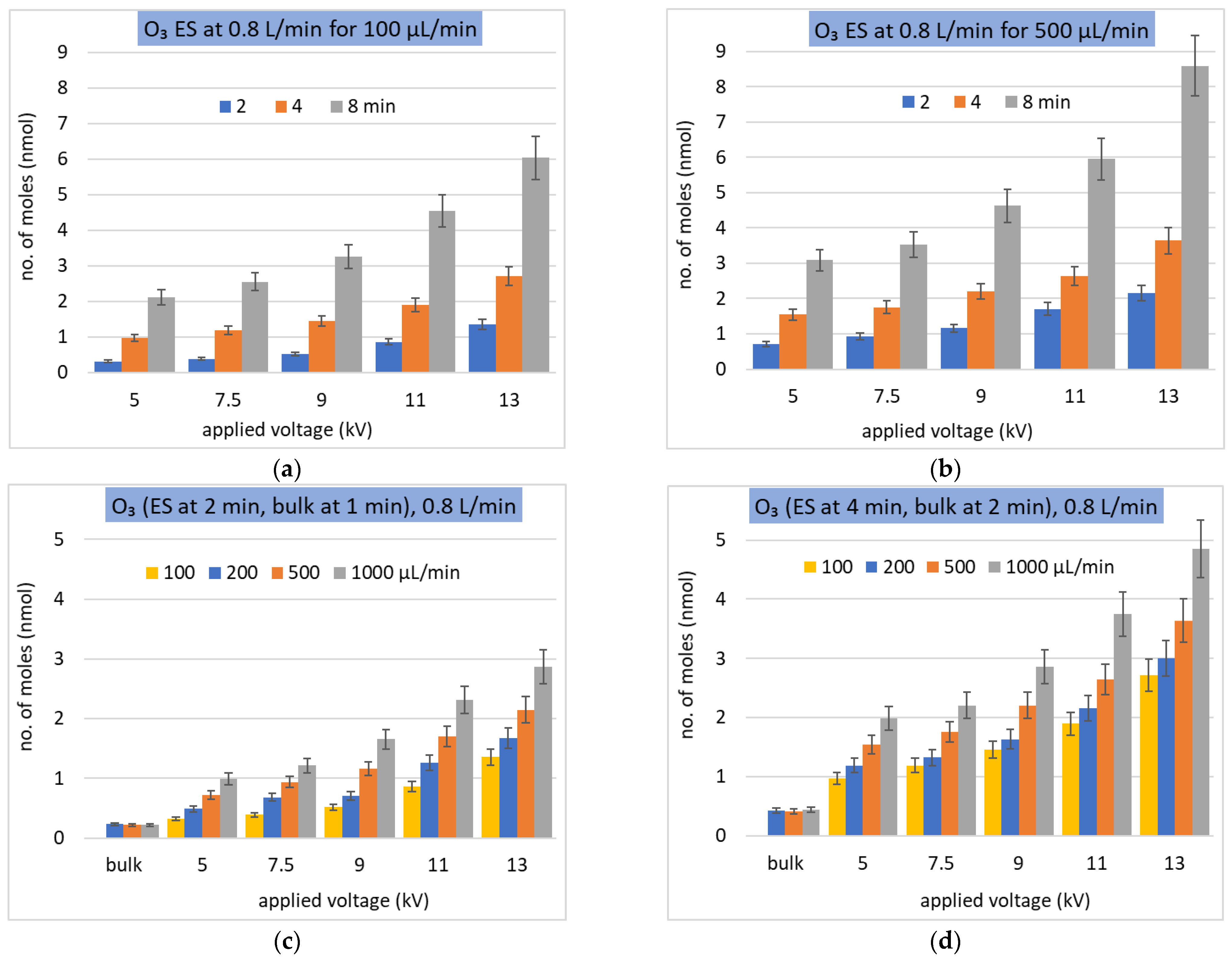
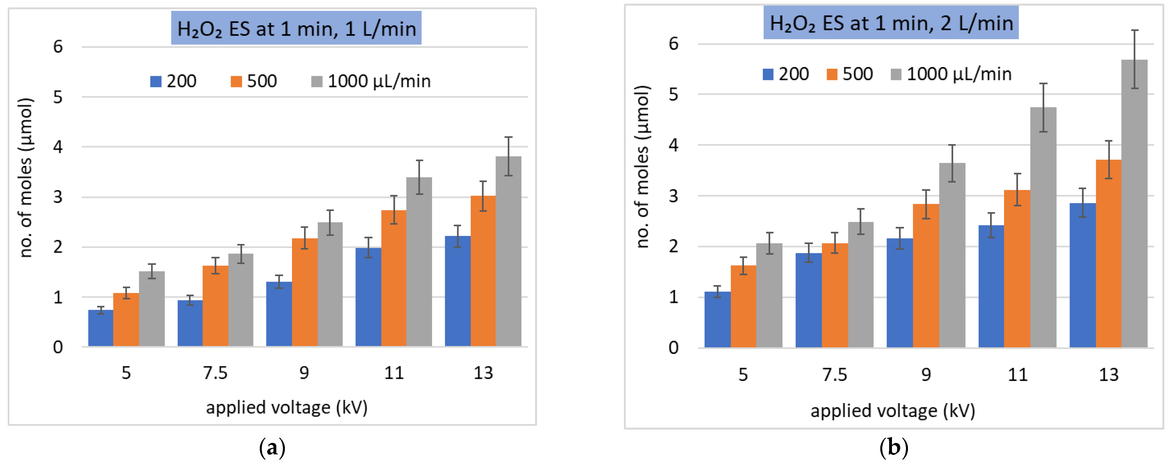
Figure 3 shows the amount of dissolved O3 and H2O2 into bulk water at various water volumes and treatment (interaction) times. Both O3 and H2O2 solvation depends almost linearly on the treatment time. It is interesting to compare the dissolved molar amounts of O3 and H2O2: while O3 dissolves at the maximum of 0.9 nmol (gas flow rate 0.8 L/min, interaction time 4 min in Figure 3a), H2O2 dissolves up to 10 µmol in Figure 3c at similar conditions. This agrees with a much higher Henry’s law coefficient of H2O2 compared to O3; however, the measured difference is just four, not seven orders of magnitude as one would expect based on the difference of .
The surface area of the bulk water was kept constant (133 mm2) for all tested volumes. No influence of the water volume (i.e., the height of the water column in the bulk reactor) was detected for the same treatment time. This also shows that the total gas–water interface surface area is the key parameter determining the solvation.
At the higher gas flow rate, the residence time of the gas inside the reactor; thus, also gas–liquid interaction time, were shorter and the amount of dissolved O3 decreased, despite the higher amount of O3 delivered into the reactor per unit time (Figure 3a,b). On the other hand, for H2O2, the higher gas flow rate resulted in slightly higher solvation, due to the higher amount of H2O2 delivered into the reactor per unit time (Figure 3c,d), despite the shorter gas–liquid interaction time.
4.2. Visualization of Electrosprayed Water Droplets
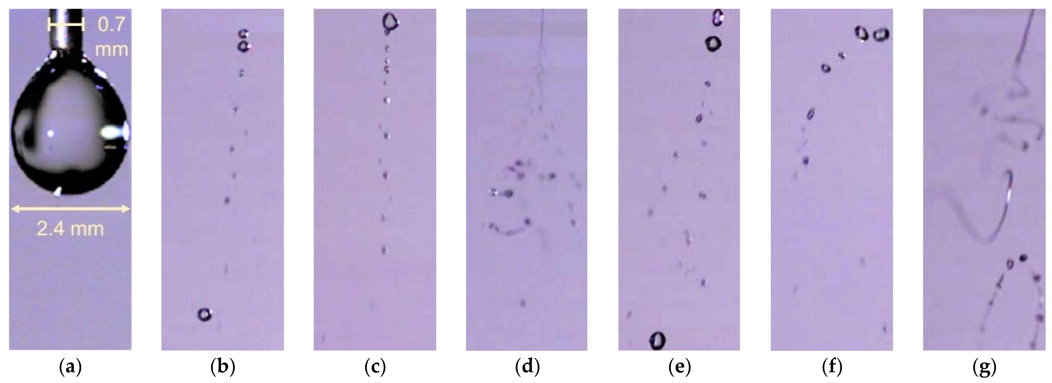
When a high voltage (Va) is applied on the needle nozzle through which the water is delivered to the reactor with a water flow rate (Qw), the ES starts at 7.5 kV (at the lower Qw) while the dc corona discharge plasma onset occurs at 9 kV. Figure 4 shows an example of electrosprayed microdroplets obtained by HS camera imaging. From a large set of HS camera images, the size distribution of the ES water microdroplets (Figure 5) is estimated. In addition to Va (Figure 5a), Qw also influences this size distribution (Figure 5b). However, the differences do not seem to be very significant. In all histograms, the largest number of droplets have a diameter around 50 µm and there are only a few droplets with a diameter above ~150 µm. The abundance of these “big” droplets slightly decreases with increasing Va and decreasing Qw.
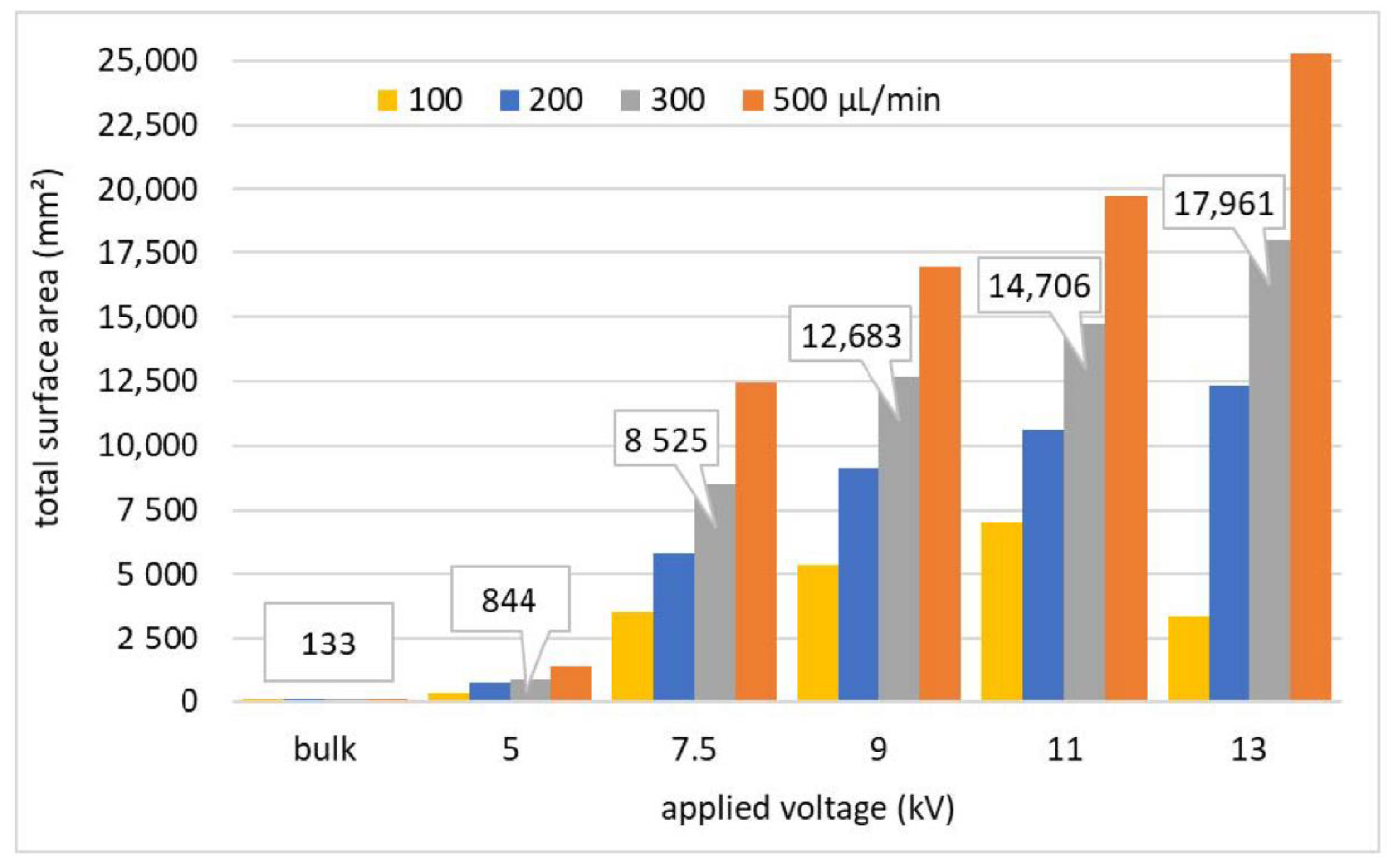
Next, the total surface area of the water ES droplets integrated for 1 min was estimated from the droplet size distributions. Figure 6 shows this total surface area for different Qw as a function of Va and it is compared with the surface area of the bulk water and water droplets (with diameter 1.5–2 mm) at 5 kV. There is a significant increase with increasing Va and Qw. At 13 kV and 500 µL/min for 1 min, the produced total surface area is almost 190 times larger than the area in the bulk liquid experiment.
4.3. Solvation of O3 and H2O2 in Electrosprayed Water Droplets
In coherence with the bulk water experiment, the amount of dissolved O3 and H2O2 into ES droplets increases with the treatment time, as shown in Figure 7a,b for O3, and Figure 8b,c for H2O2. However, this solvation rate is slower than linearly proportional with time, as observed in the bulk water experiment. The dissolved O3 and H2O2 also increase with increasing Va and Qw (Figure 7c,d for O3 and Figure 8a,b for H2O2), although the effect of increasing Qw is not so significant in some cases.
Similar to the bulk experiment, the amount of dissolved H2O2 is much higher than that of O3, but not by seven orders of magnitude, as could be expected from the ratio of their Henry’s law coefficients. In order to understand it, the number of molecules in the gas available for solvation in the liquid must be considered, and the number needed to achieve the saturated concentration cisatur. (index i denotes the i-th species, in this case H2O2 or O3). The O3 solubility is low and there are enough species in the gas phase to achieve the saturated concentration in the water, i.e., the saturation degree ξi defined as ξi(t) = ci(t)/cisatur, can approach one, without significant depletion of O3 gas density. It should be noted that the decrease of O3 concentration in the gas phase was not measurable at the resolution of 0.3 ppm by the used O3 gas sensor.
On the other hand, a measurable depletion of H2O2 in the gas phase was observed, both in the bulk and ES experiments. This is in agreement with the modeling results presented in [57,58]. The measured molar amount (number of moles) of dissolved H2O2 fits well with the molar amount of H2O2 depleted from the gas phase (Figure 8c,d) within the experimental uncertainty. The insufficient amount of H2O2 remaining in the gas phase is the factor limiting the H2O2 concentration achievable in the liquid phase.
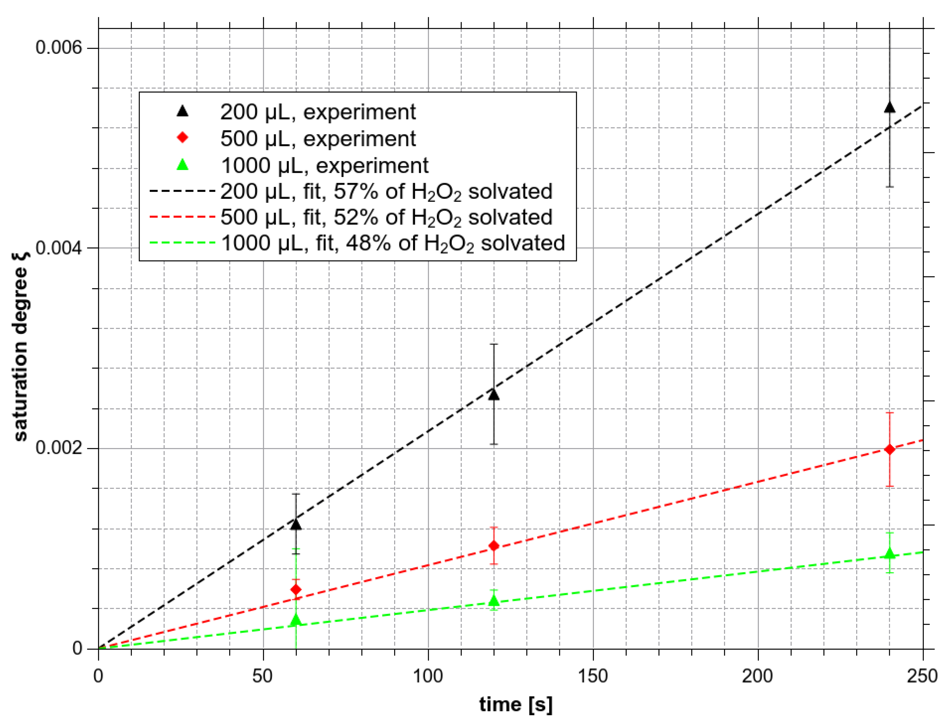
There are simply not enough H2O2 molecules in the gas phase to reach the saturated concentration in water. The saturated H2O2 concentration in liquid water is ~10 M. With the gaseous concentration of H2O2 ~100 ppm (~2.46 × 1015 cm−3), approximately 6 × 10²¹ molecules must be dissolved to achieve saturation in the used reactor and more than 2 × 10³ L of the gas passing through the reactor would be needed. With the gas flow of 1 L/min at input concentration 100 ppm, even if assumed that all H2O2 is dissolved and nothing leaves out from the reactor, such an experiment would take more than 30 h. During the experiment with 2 min treatment time, the highest achievable concentration is thus in the order of 10−3 of the saturated concentration, i.e., the H2O2 saturation degree ξH2O2 reaches the order of 0.001 only (Figure 9).
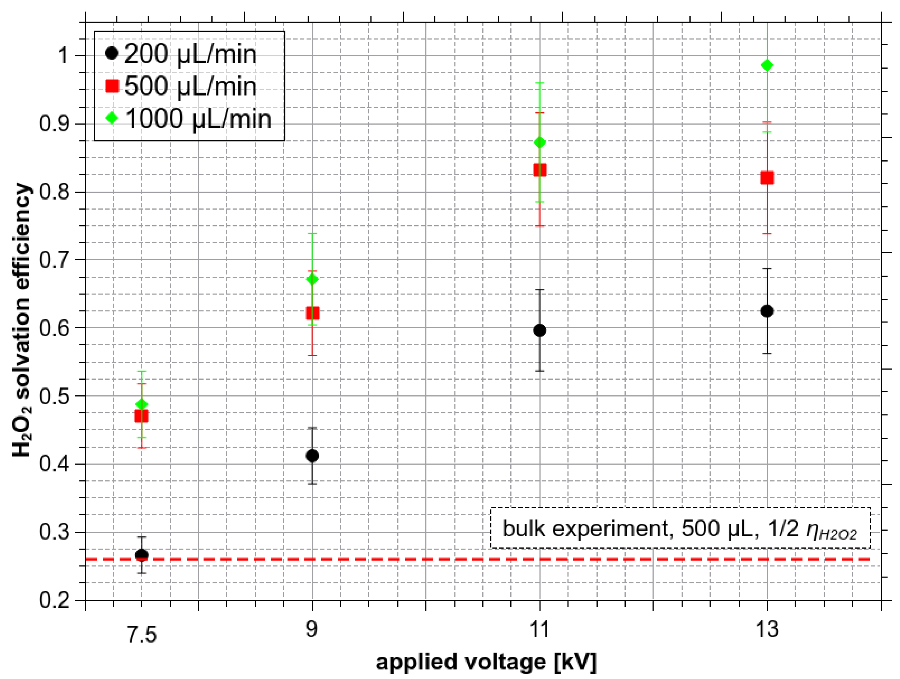
In reality, not all of the H2O2 molecules passing through the reactor can be dissolved. The solvation efficiency ηH2O2, which determines how many of the total H2O2 molecules from the gas are dissolved with respect to all available H2O2 molecules, was as high as 0.5 in the bulk experiment. This result indicates that H2O2 is well soluble even in bulk water and so it is not possible to increase it substantially by the ES. Figure 10 shows the solvation efficiency obtained in the H2O2 ES experiment with Qw 200, 500, and 1000 µL/min, treatment time 1 min, at the gas flow rate 1 L/min. If the bulk liquid experiment with 500 µL of water where ηH2O2 ≈ 0.52 is compared with the ES experiment (Figure 10), at 7.5 kV and Qw = 500 µL/min, the solvation efficiency is also only around 0.5.
However, it should be emphasized that in the ES experiments, the water is sprayed into the reactor gradually, while in the bulk experiments all the water is inside the reactor all the time since the start. The average time during the water is exposed to the gaseous H2O2 in the ES experiment is only a half of the treatment time of the bulk experiment. Thus, it is more reasonable to compare the solvation efficiency from the ES experiments with a half of the solvation efficiency obtained in the bulk liquid experiments (Figure 10). Thus, even at low voltage 7.5 kV, the enhancement of H2O2 solvation was achieved in the ES compared to the bulk.
Even if ES solvation efficiency is compared to a half of the bulk solvation efficiency (~0.25), the maximum theoretical achievable enhancement by the ES is by a factor of four. The full potential of solvation enhancement by microdroplets cannot be therefore demonstrated on H2O2 due to its extremely high solubility, causing its depletion in the gas phase and achieving 50% solvation efficiency even in the bulk experiment. In the next sections, the focus will be therefore on the O3 molecule with poor solubility, where a higher increase of the dissolved molecules was achieved in the ES (Figure 7c,d).
The highest O3 concentration in water was obtained in the ES experiment at Qw = 1000 μL/min, where ~10 times more O3 was dissolved compared to the bulk liquid experiment. However, the total interface area of microdroplets was augmented much more (the highest measured total surface area augmentation factor was 190 at 13 kV and 500 µL/min). This means that the surface area augmentation is not the only important parameter to be considered when comparing the ES and the bulk liquid solvation. Another important parameter is the interaction time.
During the ES process, the microdroplets fly from the needle nozzle towards the bottom of the reactor. Thus, the relevant lifetime of the microdroplets is not the duration of the experiment, but the time between their formation and the moment when they hit the bottom of the reactor. The lifetime of these microdroplets can be calculated from their traveled path and their speed vd. Figure 11 shows the distribution of their speed as a function of their diameter, as measured by the HS camera. The shortest possible path of a droplet moving perpendicularly to the ground is 2.5 cm, but the real path of a droplet deviated from the axis of the reactor can be as long as ~3 cm. For the biggest and the slowest microdroplets (vd ~ 3.5 m/s), the longest lifetime up to ~9 ms can be reached.
Compared to the interaction (i.e., treatment) time in the bulk experiment (1–4 min, i.e., order of 100 s), the lifetime of flying microdroplets is by 4–5 orders of magnitude shorter. Considering that the total surface area of ES microdroplets is augmented much less compared to the bulk with respect to their much shorter lifetime, one should in fact expect a lower amount of dissolved O3 into the ES droplets than in the bulk water. This contradicts the experimental results. To resolve this problem, it is necessary to consider the effect of microdroplets which stay as separated microdroplets for a certain time even after they hit the bottom of the reactor. They can stay at the bottom for a much longer time than just a few milliseconds before they merge to form bigger droplets and eventually a uniform bulk liquid.
In the real ES experiment with a constant Qw running for a specific treatment time, the total amount of dissolved O3 (and H2O2) molecules is given by the sum of those dissolved during the short lifetime of flying microdroplets, then the molecules absorbed by microdroplets sitting at the bottom of the reactor, and finally by merged bigger droplets (eventually forming bulk liquid) formed later during the experiment. There are also some microdroplets sprayed onto the walls of the reactor during the ES process. The amount of these sprayed droplets is increased with the increase of Qw, Va, and the treatment time. Contribution of various phases (flying, bottom, and sprayed droplets, besides the formed bulk) to O3 solvation into the liquid water will be discussed in the next subsection, based on a comparison of theoretical calculations with the experimental results.
4.4. Mass Transfer of Ozone from Gas to the Liquid Phase. The Role of Surface Area
In the simplified theory outlined in Section 2, Equation (8) which can be used to describe the dynamics of the microdroplets solvation was derived. Equation (8) is valid both for bulk liquid as well as for microdroplets. If only spherical droplets with diameter dk, are considered, an expression where mO3 is the mass of O3 molecules and τ is characteristic Henry’s law equilibration time can be finally derived:
It shows that the aqueous ozone concentration converges towards a saturated concentration with the increasing time. In the simplified theory used to derive this equation, it was assumed that the partial pressure of O3 did not change in time and that the concentration in the liquid phase was homogeneous. The real situation is more complicated, and this simple solvation theory is not sufficient. Equation (9) predicts very fast saturation of water by dissolved ozone even for large droplets with dk = 3 mm. The characteristic Henry’s law equilibration time predicted by this theory is much shorter than τ obtained by the more sophisticated model presented by Kruzselnicki et al. [57].
The first assumption in this model, the constant density of O3 in the gas phase, is in agreement with the results presented in the literature [57,58]. For this reason, the major problem of the above theoretical considerations was supposed as the assumption that the dissolved molecules spread immediately inside the entire droplet. It is probably only a thin gas/liquid interface, with a characteristic width of several nanometers [62,63,64,65], that becomes saturated quickly. To correct this theory, the fact that the dissolved O3 concentration inside the liquid equalizes only very slowly by diffusion must be accounted for. First, the solvation with diffusion into the bulk liquid will be discussed, where the calculations are simpler because it can be considered as a one-dimensional problem.
4.4.1. O3 Diffusion into the Bulk Liquid
In a one-dimensional situation (bulk liquid) the distance L to which O3 will diffuse during a given time can be estimated by a simple equation
where DO3 is the diffusion coefficient of O3 in water. At 300 K, DO3 = 2 × 10⁻⁵ cm2/s [66]. To simplify the calculation, it can be assumed that the surface area is quickly saturated by dissolved O3 molecules and their concentration there can be considered as constant (). The one-dimensional theory of diffusion can be used to describe the concentration evolution in time and depth h of the bulk liquid.
Integration from 0 to H (the total depth of the bulk liquid) gives the average concentration in each time, and hence the degree of saturation ξO3 as a function of time and H (Equation (12))
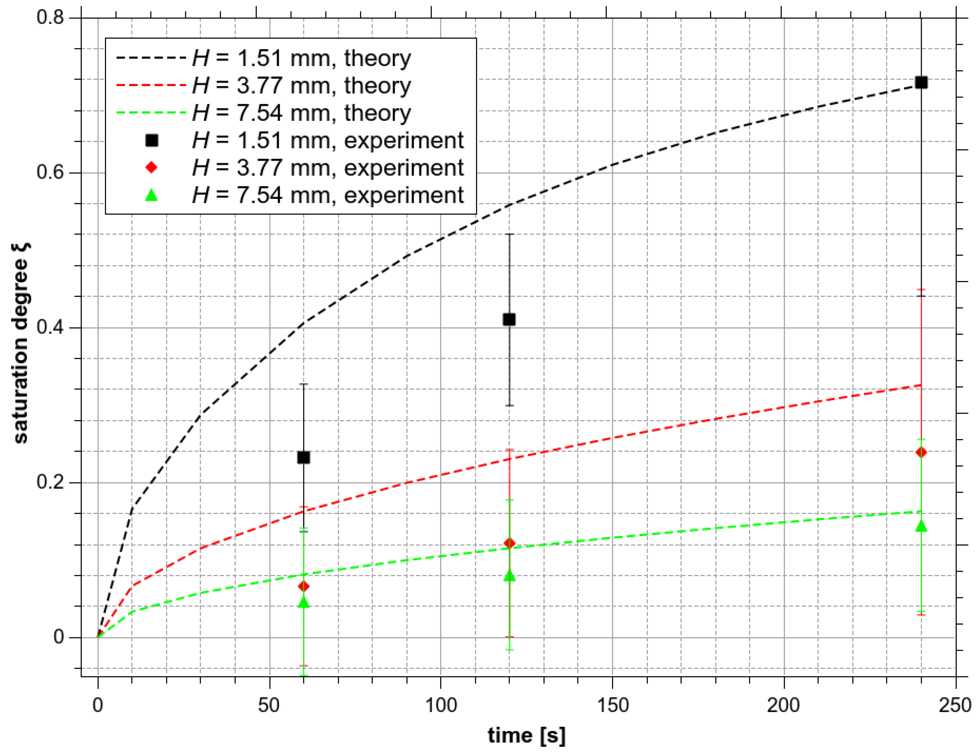
Figure 12 shows the calculated saturation degree time evolutions for three different values of the bulk water depths H: 1.51, 3.77, and 7.54 mm (they correspond to the water volumes 200, 500, and 1000 µL in the bulk reactor, respectively). With H = 3.77 mm and the treatment time 4 min (240 s), the theoretical average concentration of O3 should reach only about 32% of the saturation level. For H = 7.54 mm, this number is even lower (16%). The theoretical curves are compared with experimental results in Figure 12. There is a relatively good agreement within the experimental uncertainty, except for H = 1.51 mm, where experimental values are below the theoretical ones. At H = 1.51 mm the volume of water is very small (200 µm). Even slight vibrations and shivering of the water surface due to the gas flow can have a significant influence on the O3 solvation inside the bulk liquid.
4.4.2. O3 Diffusion into Microdroplets
Like in the bulk liquid, the calculation in ES microdroplets is easier under an assumption that the surface area is quickly saturated by O3 molecules and the concentration here can be considered as constant (). Next, the saturation degree ξO3 in the droplets as a function of time and rk (droplet radius) is estimated. The concentration of dissolved O3 inside the droplet as a function of time and a radial coordinate r is approximated by the function
The saturation degree by ozone ξO3 as a function of time and rk in spherical coordinates can be then calculated by Equation (14)
Figure S1 (Supplementary Materials) shows the estimated O3 saturation degree for flying microdroplets with different diameters in the time scale up to 10 ms, which is approximately the longest expected lifetime of the generated microdroplets (Figure 11). The increase of ξO3 calculated by Equation (14) (Figure S1) can be approximated by a formula equivalent to Equation (9) with much longer characteristic Henry’s law equilibration time τ. Kruzselnicki et al. calculated τ to be approximately 30, 100, and 300 µs for microdroplets with diameters 30, 100, and 300 µm, respectively [57]. The values obtained by our approach are approximately one order of magnitude higher. However, characteristic Henry’s law equilibration time τ from the model of Kruzselnicki et al. [57] is not in good agreement with the presented experimental data. The microdroplets lifetime above 1 ms (Figure S1) was observed and almost all of them had a diameter below 300 µm (Figure 5). According to τ from the model of [57], microdroplets would be saturated by O3 relatively shortly after the moment when they are created, long before they hit the reactor bottom. In such a case, water saturated by O3 would be always collected and no dependence of the measured O3 concentration in the water on the applied voltage and water flow rate would be detected (Figure 7). It can be thus assumed that our estimate of τ supported by the experiments is more realistic.
Based on the obtained results (Figure S1), it can be concluded that only very small microdroplets with a diameter below ~40 µm could be saturated within this timescale of ~10 ms. To achieve the highest solvation rate, it would be preferable if all droplets had this or a lower diameter. The obtained measurements show that most of the detected droplets have a slightly larger diameter, around 50 µm (Figure 5). In real ES, the average size of the microdroplets might be even smaller, because it was not possible to detect droplets with a diameter below ~20 µm by the used imaging technique with the resolution of 21.875 µm/pixel.
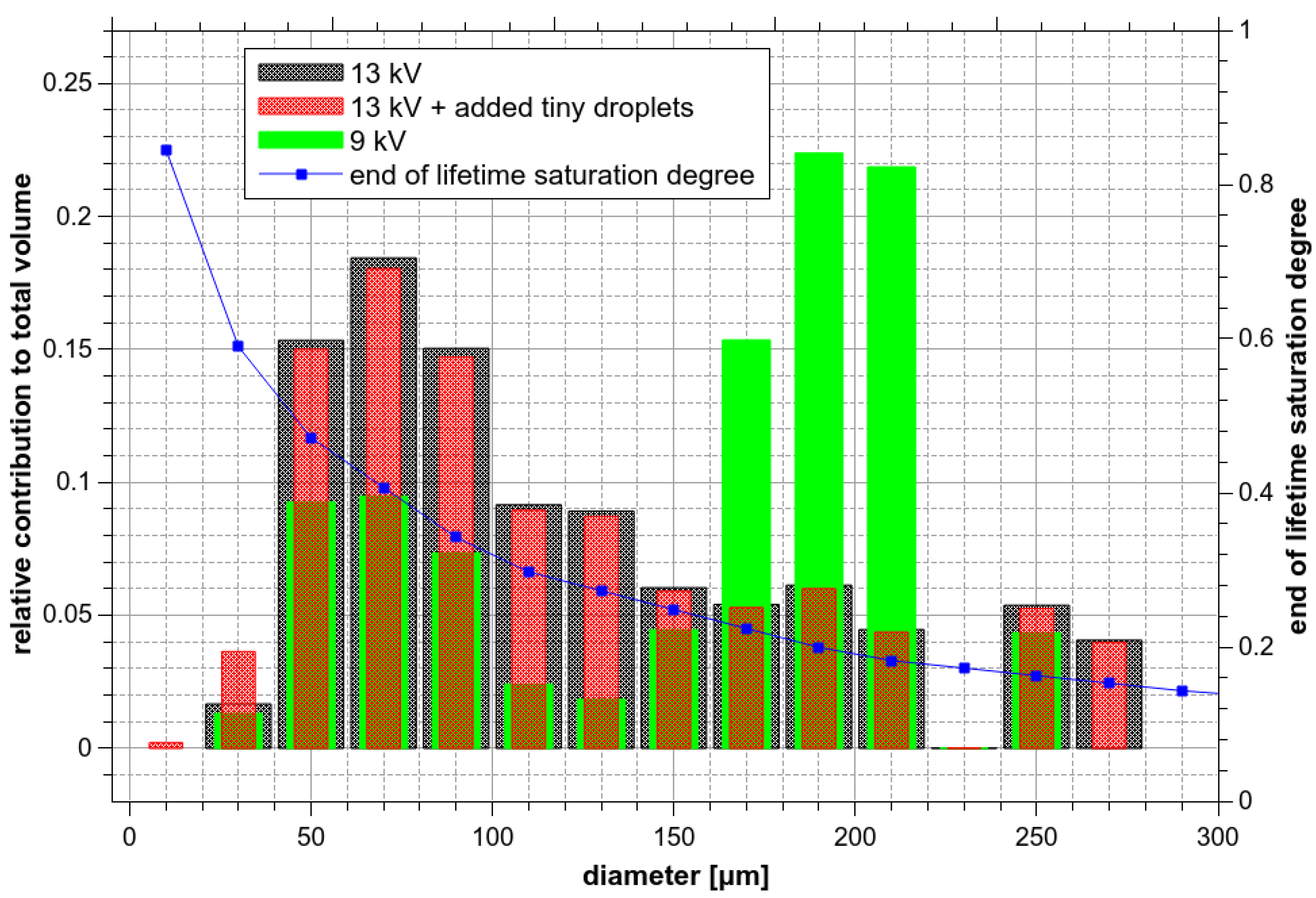
However, the droplet size distribution histograms shown in Figure 5 do not reflect that the overall saturation degree depends significantly on the volume of droplets. If 10 tiny ozone-saturated droplets (dk = 10 µm) were merged with 1 larger droplet with dk = 200 µm and ξO3 = 0.1, the resulting ξO3 would be only 0.100125, i.e., dominated by the large droplet. For this reason, data from Figure 5a have been recalculated to show the relative contribution of droplets with different diameters to the total volume Pv(dk). In this representation (Figure 13), the contribution of the tiny droplets is minimal.
For verification, the size distribution histogram measured at 13 kV and 300 µL/min was artificially modified. The number of small microdroplets with a diameter of 20–40 µm was doubled and droplets with a diameter below 20 µm were added as if their relative abundance were ~37%. Nevertheless, the influence of this modification on Pv(dk) was almost negligible (Figure 13). A significant difference between Pv(dk) at 9 and 13 kV can be seen, although the difference between 9 and 13 kV seemed to be negligible in the original droplet size distribution histogram (Figure 5a).
Figure 13 also shows ξfin(dk), the saturation degree of O3 at the end of the droplet lifetime (Figure 11, path 3 cm) as a function of droplets diameter. Finally, the effective saturation degree ξeff of droplets hitting the bottom of the reactor can be defined by integrating the product of Pv(dk) with ξfin(dk) over the entire range of diameters:
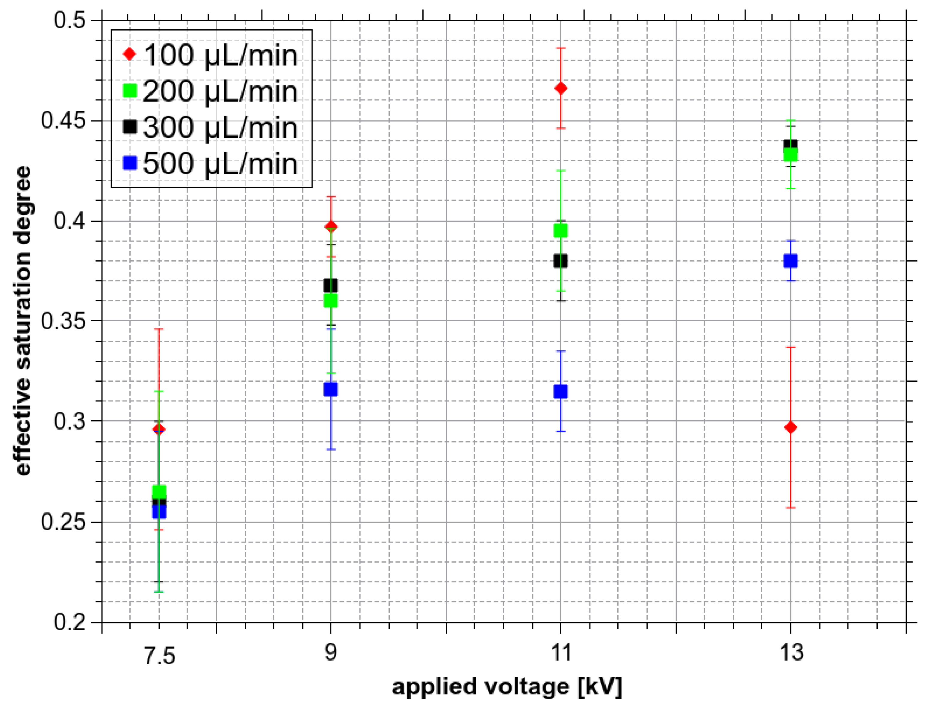
Figure 14 shows the ξeff calculated for all Va and Qw, which increases with the applied voltage that shifts the relative contribution distribution towards the smaller diameter droplets (Figure 13). As Figure 14 shows, there is no significant dependence of ξeff on the Qw, though ξeff is probably slightly smaller at 500 µL/min than at lower Qw. This could mean slightly bigger droplets on average. On the other hand, ξeff calculated at 100 µL/min is probably slightly higher than at higher Qw, except for Va = 13 kV, when the formation of microdroplets was most probably influenced by the onset of corona discharge. The increase of ξeff with increasing Va can partly explain the increase of the dissolved O3 amount with increasing Va (Figure 7). For a more precise explanation of the observed dependence of solvation on Va, the microdroplets sitting at the bottom must be also considered.
To estimate the role of microdroplets sitting at the bottom of the reactor, some simplifications should be considered. We will consider these bottom microdroplets to be semi-spheres (with a contact angle 90°) having the same volume as their parent microdroplets from the ES. Consequently, their diameter ds will be slightly bigger than the diameter of their parent microdroplets (ds ~1.26 dk). Next, the saturation degree reached in these bottom microdroplets can be estimated if their lifetime (τs) is known. Water flow rate Qw is constant during the experiment and if they do not coagulate, their average lifetime would be equal to half of the total treatment time. Thus, for the Qw of 200 µL/min, the total water volume 1 mL would be collected at the bottom in 5 min (300 s) and the average lifetime of bottom microdroplets would be 150 s.
In the ES experiment, the droplets are sprayed into a relatively wide solid angle. As a result, they are distributed all over the reactor bottom (even walls) in the initial phase. Gradually, bigger droplets are being formed at places with the highest flux of merging droplets. This process decreases the average lifetime of bottom microdroplets. Moreover, as the reactor bottom gets gradually more and more covered by big droplets, more and more incoming microdroplets hit these big droplets instead of the clean surface of the reactor bottom, having thus the bottom lifetime τs = 0 s. A correct assessment of the bottom droplets′ lifetime will require further studies. Here, as the first approximation, the saturation degree of the bottom microdroplets using τs up to 10 s was calculated from Equation (14). For ds = 300 µm (corresponding to the parent microdroplets with dk = 238 µm), it is obtained that the saturation degree will exceed 90% within τs = 10 s, even starting from the saturation degree 0 (Figure S2 in Supplementary Materials). This shows that the solvation into bottom microdroplets plays a significant role in the experiment, even if their average lifetime is in the order of 1 s, which is still much longer than the lifetime of flying microdroplets (~10 ms).
4.4.3. Roles of Flying Microdroplets, Sitting Bottom Microdroplets vs. Solvation in the Formed Bulk
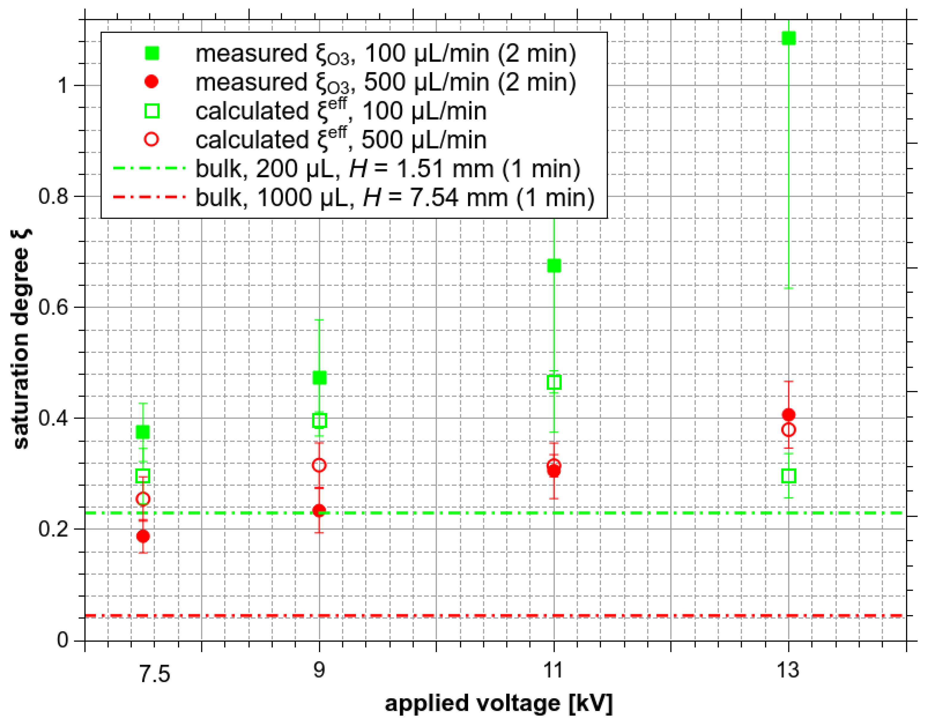
The calculated effective saturation degree ξeff of flying microdroplets (Figure 14) could help to assess the importance of flying microdroplets vs. sitting bottom microdroplets vs. formed bulk water solvation of O3. ξeff to the measured ξO3 values should be compared under various experimental conditions. It is demonstrated in Figure 15.
First, by looking at the ES experiment with Qw of 500 µL/min and a treatment time of 2 min, the total amount of collected water is 1000 µL. Qw is relatively high, and the bulk liquid is quickly formed and then exists during most of the treatment time. The contribution of bottom microdroplets should be thus small. The contribution of the solvation in the formed bulk can be estimated from the experiment with bulk water with volume 1000 µL (H = 7.54 mm) and the duration 1 min (half of the ES experiment time, because in the ES experiment the average water residence time inside the reactor is half of the treatment time), where the saturation degree only around 0.045 was achieved (red dashed line at the bottom of Figure 15). Thus, in the ES experiment even at low Va = 7.5 kV, where ξO3 is significantly higher (~0.25) than in the bulk (0.045), the saturation must be mostly achieved, thanks to the flying microdroplets. This can explain a good correlation between the measured ξO3 and ξeff for Qw = 500 µL/min in Figure 15.
Second, let us consider the ES experiment with the Qw only 100 µL/min, with no formed bulk and no big droplets formation during most of the treatment time. Thus, the contribution of bottom droplets should be crucial, while the contribution of the O3 solvation into the formed bulk should be small, although, in the bulk water experiment with the volume 200 µL (H = 1.51 mm) and duration 1 min, the saturation degree ξO3 ≈ 0.23 was achieved. In the ES experiment, even at low Va 7.5 kV, ξO3 reached almost 0.4. The formed bulk solvation contribution would be even less important at higher Va, where the advantage of flying and bottom microdroplets is already clearly visible because ξO3 grows with increasing Va up to 1.12 ± 0.57. When comparing the ES experiment with Qw = 500 µL/min and 100 µL/min, the significant increase of ξO3 should be mostly due to the sitting bottom droplets. This also explains a high experimental uncertainty of the measured ξO3. The coagulation of microdroplets and big droplet formation is significantly different in each individual experiment.
5. Conclusions
Motivated by the increasing interest in plasma–liquid interactions and their applications, and knowledge gaps in the detailed understanding of the reactive species transport into liquids, the objective of this article was to investigate the transport of the most typical air plasma reactive species (O3 and H2O2) into water. Solvation experiments with single O3 and H2O2 species in the airflow were conducted and their transport into bulk water vs. electrosprayed aerosol microdroplets was analyzed.
The gas–water interface surface area and the treatment (interaction) time are shown to be the key parameters of determining the amount of dissolved O3 and H2O2 in the bulk water regardless of the water volume. About 104 times more H2O2 than O3 was dissolved in the water despite the 107 times larger Henry’s law coefficient of H2O2 than that of O3. This is because the amount of gaseous H2O2 molecules next to the gas–water interface area, unlike O3 molecules, is strongly depleted.
The total surface area of electrosprayed water microdroplets and thus the dissolved O3 and H2O2 increased with the increasing applied voltage and water flow rate. However, the observed solvation effect cannot be explained simply by the measured droplet size distribution and their total surface area. The limitation in the ES experiment is a very short lifetime (up to 9 ms only) of the generated flying microdroplets. In addition to this very short flying phase of the ES microdroplets, other phases of their total interaction time with O3 and H2O2, such as microdroplets sitting at the reactor bottom (and walls) until they merge and progressively form the bulk strongly contribute to the solvation of O3 and H2O2 into the ES water.
The experimental results were confronted with simple theoretical considerations. For O3, where no significant depletion of the gaseous molecules occurs, the diffusion of dissolved O3 molecules inside the liquid limits the solvation. After accounting for this diffusion in the liquid, a reasonable agreement of the saturation time evolution was achieved with the bulk liquid experiment. For O3 solvation in electrosprayed water microdroplets, their lifetime, as well as their contribution to the total water volume depending on their size and abundance are the most important parameters. At all water flow rates, ES water microdroplets (both flying and bottom) play the key roles in the total solvation.
In summary, we experimentally demonstrated and theoretically explained that Henry′s law coefficient is not the only important parameter determining the dissolution of highly and lowly soluble (H2O2 and O3) gaseous species into the water. Other experimental parameters, such as the gas–liquid interface surface area, gas flow rate, and the treatment (interaction) time should be considered for their solvation in the bulk liquid. In the ES microdroplets, the applied voltage, the water flow rate, and the microdroplet contribution to the total water volume are important, too. Their roles on flying and bottom microdroplets and the formed bulk were established. However, more detailed experimental/theoretical studies of these individual phenomena influencing water solvation of each specific species are needed in the future.
The investigated physical parameters allow for controlling the solvation efficiency of H2O2 and O3 gases into water bulk and electrospray. Our findings contribute to a better understanding of the solvation process of different gaseous species and can lead to optimization of the water spray systems and plasma–water interaction systems and their working conditions for multiple applications. The results can be useful e.g., when designing water ozonizers that cope with a low and relatively slow O3 solvation: spraying water to fine aerosol microdroplets and extending their interaction time with the gaseous O3 results in more efficient O3 mass transfer. On the other hand, in plasma–liquid interactions and plasma-activated water production systems, it is important to dissolve the maximum of the available H2O2 with typically low gaseous concentrations and reach the highest possible H2O2 concentrations in the water. H2O2 saturation in water can be only reached in the optimized reactor with a strong H2O2 depletion from the gas using a minimal volume of aerosolized water.
Supplementary Materials
The following are available online at https://www.mdpi.com/2073-4441/13/2/182/s1, Figure S1: Estimated evolution of saturation degree ξO3 of O3 as a function of time and diameter of flying microdroplets dk, calculated for O3 diffusion in the water microdroplets at 300 K, time span up to 10 ms. Figure S2: Estimated evolution of saturation degree ξO3 as a function of time and diameter of sitting bottom microdroplets ds, calculated for O3 diffusion in the water at 300 K, time span up to 10 s.
Author Contributions
M.E.H. ran and processed the experiments with microdroplets by fast/HS camera, and the investigations of H2O2 and O3 solvation into bulk and electrosprayed water, and wrote the first draft of the manuscript; M.J. contributed to the microdroplet visualization experiments and wrote the theoretical parts in the results and discussion including the comparison of the experimental and theoretical results; Z.M. planned, organized, and supervised the research, and reviewed and edited the manuscript. All authors have read and agreed to the published version of the manuscript.
Funding
This work was supported by Slovak Research and Development Agency APVV-17-0382, APVV-0134-12 and SK-PL-18-0090, Slovak Grant Agency VEGA 1/0419/18, and Comenius University grants UK/317/2020 and UK/325/2019.
Institutional Review Board Statement
Not applicable.
Informed Consent Statement
Not applicable.
Data Availability Statement
Not applicable.
Acknowledgments
We thank Piotr Terebun, Michal Kwiatkowski, and Joanna Pawlat from Lublin University of Technology, Poland, for enabling us HS camera measurements.
Conflicts of Interest
The authors declare no conflict of interest in publishing this manuscript.
Abbreviations
| PAW | plasma-activated water |
| RONS | reactive oxygen and nitrogen species |
| ES | electrospray |
| Henry’s law solubility coefficient | |
| molar concentration of i-species in the aqueous phase | |
| partial pressure of i-species in the gas phase | |
| molar concentration of i-species in the gas phase | |
| PTFE | polytetrafluoroethylene-flexible teflon tube |
| w/w | weight by weight |
| ppm | parts-per-million |
| H | water depth |
| dc | direct current |
| HV | high voltage |
| fps | frame per second |
| Va | applied high voltage |
| Qw | water flow rate |
| vd | speed of flying microdroplets |
| dk | diameter of microdroplet |
| τ | characteristic Henry’s law equilibration time |
| ξO3 | saturation degree by ozone |
| Pv(dk) | total volume of droplets with different diameters |
| ξeff | effective saturation degree of droplets |
| ds | diameter of bottom microdroplets |
| τs | lifetime of bottom microdroplets |
References
- Bruggeman, P.; Leys, C. Non-thermal plasmas in and in contact with liquids. J. Phys. D Appl. Phys. 2009, 42, 053001. [Google Scholar] [CrossRef]
- Rezaei, F.; Vanraes, P.; Nikiforov, A.; Morent, R.; De Geyter, N. Applications of Plasma-Liquid Systems: A Review. Materials 2019, 12, 2751. [Google Scholar] [CrossRef] [PubMed] [Green Version]
- Bruggeman, P.J.; Kushner, M.J.; Locke, B.R.; Gardeniers, J.G.E.; Graham, W.G.; Graves, D.B.; Hofman-Caris, R.C.H.M.; Maric, D.; Reid, J.P.; Ceriani, E.; et al. Plasma-liquid interactions: A review and roadmap. Plasma Sources Sci. Technol. 2016, 25, 053002. [Google Scholar] [CrossRef]
- Locke, B.R.; Sato, M.; Sunka, P.; Hoffmann, M.R.; Chang, J.S. Electrohydraulic discharge and nonthermal plasma for water treatment. Ind. Eng. Chem. Res. 2006, 45, 882–905. [Google Scholar] [CrossRef]
- Locke, B.R. Environmental Applications of Electrical Discharge Plasma with Liquid Water—A Mini Review. Int. J. Plasma Environ. Sci. Technol. 2012, 6, 194–203. [Google Scholar]
- Chen, Q.; Li, J.; Li, Y. A review of plasma-liquid interactions for nanomaterial synthesis. J. Phys. D Appl. Phys. 2015, 48, 424005. [Google Scholar] [CrossRef] [Green Version]
- Machala, Z.; Hensel, K.; Akishev, Y. (Eds.) Plasma for Bio-Decontamination, Medicine and Food Security; NATO Science for Peace and Security Series A: Chemistry and Biology; Springer: Dordrecht, The Netherlands, 2012; ISBN 978-94-007-2851-6. [Google Scholar]
- Von Woedtke, T.; Schmidt, A.; Bekeschus, S.; Wende, K.; Weltmann, K.D. Plasma medicine: A field of applied redox biology. In Vivo 2019, 33, 1011–1026. [Google Scholar] [CrossRef] [PubMed] [Green Version]
- Vanraes, P.; Bogaerts, A. Plasma physics of liquids—A focused review. Appl. Phys. Rev. 2018, 5, 031103. [Google Scholar] [CrossRef]
- Kong, M.G.; Kroesen, G.; Morfill, G.; Nosenko, T.; Shimizu, T.; van Dijk, J.; Zimmermann, J.L. Plasma medicine: An introductory review. New J. Phys. 2009, 11, 115012. [Google Scholar] [CrossRef]
- Fridman, G.; Friedman, G.; Gutsol, A.; Shekhter, A.B.; Vasilets, V.N.; Fridman, A. Applied Plasma Medicine. Plasma Process. Polym. 2008, 5, 503–533. [Google Scholar] [CrossRef]
- Laroussi, M. Low-Temperature Plasmas for Medicine? IEEE Trans. Plasma Sci. 2009, 37, 714–725. [Google Scholar] [CrossRef]
- Šimončicová, J.; Kryštofová, S.; Medvecká, V.; Ďurišová, K.; Kaliňáková, B. Technical applications of plasma treatments: Current state and perspectives. Appl. Microbiol. Biotechnol. 2019, 103, 5117–5129. [Google Scholar] [CrossRef] [PubMed]
- Laroussi, M.; Kong, M.; Morfill, G.; Stolz, W. Plasma Medicine: Applications of Low-Temperature Gas Plasmas in Medicine and Biology; Cambridge University Press: Cambridge, UK, 2012; Volume 9781107006, ISBN 9780511902598. [Google Scholar]
- Fridman, A.; Friedman, G. Plasma Medicine; John Wiley and Sons: Hoboken, NJ, USA, 2013; ISBN 9780470689707. [Google Scholar]
- Fridman, G.; Peddinghaus, M.; Balasubramanian, M.; Ayan, H.; Fridman, A.; Gutsol, A.; Brooks, A. Blood Coagulation and Living Tissue Sterilization by Floating-Electrode Dielectric Barrier Discharge in Air. Plasma Chem. Plasma Process. 2006, 26, 425–442. [Google Scholar] [CrossRef]
- Dobrynin, D.; Fridman, G.; Friedman, G.; Fridman, A. Physical and biological mechanisms of direct plasma interaction with living tissue. New J. Phys. 2009, 11, 115020. [Google Scholar] [CrossRef]
- Stoffels, E.; Kieft, I.E.; Sladek, R.E.J. Superficial treatment of mammalian cells using plasma needle. J. Phys. D Appl. Phys. 2003, 36, 2908–2913. [Google Scholar] [CrossRef]
- Choi, J.; Mohamed, A.-A.H.; Kang, S.K.; Woo, K.C.; Kim, K.T.; Lee, J.K. 900-MHz Nonthermal Atmospheric Pressure Plasma Jet for Biomedical Applications. Plasma Process. Polym. 2010, 7, 258–263. [Google Scholar] [CrossRef]
- Lloyd, G.; Friedman, G.; Jafri, S.; Schultz, G.; Fridman, A.; Harding, K. Gas Plasma: Medical Uses and Developments in Wound Care. Plasma Process. Polym. 2010, 7, 194–211. [Google Scholar] [CrossRef]
- Kovalóvá, Z.; Zahoran, M.; Zahoranová, A.; Machala, Z. Streptococci biofilm decontamination on teeth by low-temperature air plasma of dc corona discharges. J. Phys. D Appl. Phys. 2014, 47, 224014. [Google Scholar] [CrossRef]
- Metelmann, H.R.; von Woedtke, T.; Weltmann, K.D. Comprehensive Clinical Plasma Medicine: Cold Physical Plasma for Medical Application; Springer International Publishing: Berlin/Heidelberg, Germany, 2018; ISBN 9783319676272. [Google Scholar]
- Parvulescu, V.I.; Magureanu, M.; Lukes, P. (Eds.) Plasma Chemistry and Catalysis in Gases and Liquids; Wiley-VCH Verlag GmbH & Co. KGaA: Weinheim, Germany, 2012; ISBN 9783527649525. [Google Scholar]
- Puač, N.; Gherardi, M.; Shiratani, M. Plasma agriculture: A rapidly emerging field. Plasma Process. Polym. 2018, 15, 1700174. [Google Scholar] [CrossRef]
- Thirumdas, R.; Kothakota, A.; Annapure, U.; Siliveru, K.; Blundell, R.; Gatt, R.; Valdramidis, V.P. Plasma activated water (PAW): Chemistry, physico-chemical properties, applications in food and agriculture. Trends Food Sci. Technol. 2018, 77, 21–31. [Google Scholar] [CrossRef]
- Ebihara, K.; Mitsugi, F.; Ikegami, T.; Nakamura, N.; Hashimoto, Y.; Yamashita, Y.; Baba, S.; Stryczewska, H.D.; Pawlat, J.; Teii, S.; et al. Ozone-mist spray sterilization for pest control in agricultural management. Eur. Phys. J. Appl. Phys. 2013, 61, 24318. [Google Scholar] [CrossRef]
- Oehmigen, K.; Hähnel, M.; Brandenburg, R.; Wilke, C.; Weltmann, K.-D.; von Woedtke, T. The Role of Acidification for Antimicrobial Activity of Atmospheric Pressure Plasma in Liquids. Plasma Process. Polym. 2010, 7, 250–257. [Google Scholar] [CrossRef]
- Graves, D.B. The emerging role of reactive oxygen and nitrogen species in redox biology and some implications for plasma applications to medicine and biology. J. Phys. D Appl. Phys. 2012, 45, 263001. [Google Scholar] [CrossRef]
- Brisset, J.L.; Pawlat, J. Chemical Effects of Air Plasma Species on Aqueous Solutes in Direct and Delayed Exposure Modes: Discharge, Post-discharge and Plasma Activated Water. Plasma Chem. Plasma Process. 2016, 36, 355–381. [Google Scholar] [CrossRef]
- Čech, J.; Stahel, P.; Ráhel, J.; Prokeš, L.; Rudolf, P.; Maršálková, E.; Maršálek, B. Mass Production of Plasma Activated Water: Case Studies of Its Biocidal Effect on Algae and Cyanobacteria. Water 2020, 12, 3167. [Google Scholar] [CrossRef]
- Machala, Z.; Tarabová, B.; Sersenová, D.; Janda, M.; Hensel, K. Chemical and antibacterial effects of plasma activated water: Correlation with gaseous and aqueous reactive oxygen and nitrogen species, plasma sources and air flow conditions. J. Phys. D Appl. Phys. 2019, 52, 034002. [Google Scholar] [CrossRef]
- Machala, Z.; Tarabova, B.; Hensel, K.; Spetlikova, E.; Sikurova, L.; Lukes, P. Formation of ROS and RNS in Water Electro-Sprayed through Transient Spark Discharge in Air and their Bactericidal Effects. Plasma Process. Polym. 2013, 10, 649–659. [Google Scholar] [CrossRef]
- Yusupov, M.; Neyts, E.C.; Simon, P.; Berdiyorov, G.; Snoeckx, R.; Van Duin, A.C.T.; Bogaerts, A. Reactive molecular dynamics simulations of oxygen species in a liquid water layer of interest for plasma medicine. J. Phys. D Appl. Phys. 2014, 47. [Google Scholar] [CrossRef] [Green Version]
- Stratton, G.R.; Bellona, C.L.; Dai, F.; Holsen, T.M.; Thagard, S.M. Plasma-based water treatment: Conception and application of a new general principle for reactor design. Chem. Eng. J. 2015, 273, 543–550. [Google Scholar] [CrossRef]
- Locke, B.R.; Shih, K.Y. Review of the methods to form hydrogen peroxide in electrical discharge plasma with liquid water. Plasma Sources Sci. Technol. 2011, 20, 034006. [Google Scholar] [CrossRef]
- Aristova, N.A.; Piskarev, I.M.; Ivanovskii, A.V.; Selemir, V.D.; Spirov, G.M.; Shlepkin, S. Initiation of chemical reactions with an electric discharge in a solid dielectric-gas-liquid system. Russ. J. Phys. Chem. A 2004, 78, 1144–1148. [Google Scholar]
- Winter, J.; Tresp, H.; Hammer, M.U.; Iseni, S.; Kupsch, S.; Schmidt-Bleker, A.; Wende, K.; Dünnbier, M.; Masur, K.; Weltmann, K.D.; et al. Tracking plasma generated H2O2 from gas into liquid phase and revealing its dominant impact on human skin cells. J. Phys. D Appl. Phys. 2014, 47, 285401. [Google Scholar] [CrossRef]
- Oinuma, G.; Nayak, G.; Du, Y.; Bruggeman, P.J. Controlled plasma-droplet interactions: A quantitative study of OH transfer in plasma-liquid interaction. Plasma Sources Sci. Technol. 2020, 29, 095002. [Google Scholar] [CrossRef]
- Burlica, R.; Grim, R.G.; Shih, K.-Y.; Balkwill, D.; Locke, B.R. Bacteria Inactivation Using Low Power Pulsed Gliding Arc Discharges with Water Spray. Plasma Process. Polym. 2010, 7, 640–649. [Google Scholar] [CrossRef]
- Kanev, I.L.; Mikheev, A.Y.; Shlyapnikov, Y.M.; Shlyapnikova, E.A.; Morozova, T.Y.; Morozov, V.N. Are Reactive Oxygen Species Generated in Electrospray at Low Currents? Anal. Chem. 2014, 86, 1511–1517. [Google Scholar] [CrossRef]
- Pyrgiotakis, G.; McDevitt, J.; Bordini, A.; Diaz, E.; Molina, R.; Watson, C.; Deloid, G.; Lenard, S.; Fix, N.; Mizuyama, Y.; et al. A chemical free, nanotechnology-based method for airborne bacterial inactivation using engineered water nanostructures. Environ. Sci. Nano 2014, 1, 15–26. [Google Scholar] [CrossRef]
- Kovalova, Z.; Leroy, M.; Kirkpatrick, M.J.; Odic, E.; Machala, Z. Corona discharges with water electrospray for Escherichia coli biofilm eradication on a surface. Bioelectrochemistry 2016, 112, 91–99. [Google Scholar] [CrossRef] [Green Version]
- Pulicharla, R.; Proulx, F.; Behmel, S.; Sérodes, J.-B.; Rodriguez, M.J. Trends in Ozonation Disinfection By-Products—Occurrence, Analysis and Toxicity of Carboxylic Acids. Water 2020, 12, 756. [Google Scholar] [CrossRef] [Green Version]
- Ferreiro, C.; Villota, N.; Lombraña, J.I.; Rivero, M.J. Heterogeneous Catalytic Ozonation of Aniline-Contaminated Waters: A Three-Phase Modelling Approach Using TiO2/GAC. Water 2020, 12, 3448. [Google Scholar] [CrossRef]
- Berry, M.; Taylor, C.; King, W.; Chew, Y.; Wenk, J. Modelling of Ozone Mass-Transfer through Non-Porous Membranes for Water Treatment. Water 2017, 9, 452. [Google Scholar] [CrossRef]
- Xia, Z.; Hu, L. Treatment of Organics Contaminated Wastewater by Ozone Micro-Nano-Bubbles. Water 2018, 11, 55. [Google Scholar] [CrossRef] [Green Version]
- Grace, J.M.; Marijnissen, J.C.M. A review of liquid atomization by electrical means. J. Aerosol Sci. 1994, 25, 1005–1019. [Google Scholar] [CrossRef]
- Borra, J.P.; Ehouarn, P.; Boulaud, D. Electrohydrodynamic atomisation of water stabilised by glow discharge—Operating range and droplet properties. J. Aerosol Sci. 2004, 35, 1313–1332. [Google Scholar] [CrossRef]
- Pongrác, B.; Kim, H.H.; Janda, M.; Martišovitš, V.; Machala, Z. Fast imaging of intermittent electrospraying of water with positive corona discharge. J. Phys. D Appl. Phys. 2014, 47, 315202. [Google Scholar] [CrossRef]
- Jaworek, A.; Sobczyk, A.; Czech, T.; Krupa, A. Corona discharge in electrospraying. J. Electrostat. 2014, 72, 166–178. [Google Scholar] [CrossRef]
- Maguire, P.D.; Mahony, C.M.O.; Kelsey, C.P.; Bingham, A.J.; Montgomery, E.P.; Bennet, E.D.; Potts, H.E.; Rutherford, D.C.E.; McDowell, D.A.; Diver, D.A.; et al. Controlled microdroplet transport in an atmospheric pressure microplasma. Appl. Phys. Lett. 2015, 106, 224101. [Google Scholar] [CrossRef] [Green Version]
- Jaworek, A.; Ganán-Calvo, A.M.; Machala, Z. Low temperature plasmas and electrosprays. J. Phys. D Appl. Phys. 2019, 52, 233001. [Google Scholar] [CrossRef]
- Borra, J.-P. Review on water electro-sprays and applications of charged drops with focus on the corona-assisted cone-jet mode for High Efficiency Air Filtration by wet electro-scrubbing of aerosols. J. Aerosol Sci. 2018, 125, 208–236. [Google Scholar] [CrossRef]
- Stancampiano, A.; Gallingani, T.; Gherardi, M.; Machala, Z.; Maguire, P.; Colombo, V.; Pouvesle, J.-M.; Robert, E. Plasma and Aerosols: Challenges, Opportunities and Perspectives. Appl. Sci. 2019, 9, 3861. [Google Scholar] [CrossRef] [Green Version]
- Sander, R. Compilation of Henry’s law coefficients (version 4.0) for water as solvent. Atmos. Chem. Phys. 2015, 15, 4399–4981. [Google Scholar] [CrossRef] [Green Version]
- Kruszelnicki, J.; Lietz, A.M.; Kushner, M.J. Interaction between atmospheric pressure plasmas and liquid microdroplets. In Proceedings of the International Conference on Plasmas with Liquids (ICPL 2017), Prague, Czech Republic, 5–9 March 2017; Lukeš, P., Koláček, K., Eds.; p. 37. [Google Scholar]
- Kruszelnicki, J.; Lietz, A.M.; Kushner, M.J. Atmospheric pressure plasma activation of water droplets. J. Phys. D Appl. Phys. 2019, 52, 355207. [Google Scholar] [CrossRef] [Green Version]
- Verlackt, C.C.W.; Van Boxem, W.; Bogaerts, A. Transport and accumulation of plasma generated species in aqueous solution. Phys. Chem. Chem. Phys. 2018, 20, 6845–6859. [Google Scholar] [CrossRef] [PubMed]
- Eisenberg, G.M. Colorimetric Determination of Hydrogen Peroxide. Ind. Eng. Chem. Anal. Ed. 1943, 15, 327–328. [Google Scholar] [CrossRef]
- Bader, H.; Hoigné, J. Determination of ozone in water by the indigo method. Water Res. 1981, 15, 449–456. [Google Scholar] [CrossRef]
- Tarabová, B.; Lukeš, P.; Janda, M.; Hensel, K.; Šikurová, L.; Machala, Z. Specificity of detection methods of nitrites and ozone in aqueous solutions activated by air plasma. Plasma Process. Polym. 2018, 15, 1800030. [Google Scholar] [CrossRef]
- Carey, V.P. Liquid-Vapor Phase-Change Phenomena; CRC Press: Boca Raton, FL, USA, 2020. [Google Scholar]
- Garrett, B.C.; Schenter, G.K.; Morita, A. Molecular simulations of the transport of molecules across the liquid/vapor interface of water. Chem. Rev. 2006, 106, 1355–1374. [Google Scholar] [CrossRef]
- Garrett, B.C. Ions at the Air/Water Interface. Science 2004, 303, 1146–1147. [Google Scholar] [CrossRef]
- Morita, A.; Garrett, B.C. Molecular theory of mass transfer kinetics and dynamics at gas-water interface. Fluid Dyn. Res. 2008, 40, 459–473. [Google Scholar] [CrossRef]
- Johnson, P.N.; Davis, R.A. Diffusivity of ozone in water. J. Chem. Eng. Data 1996, 41, 1485–1487. [Google Scholar] [CrossRef]
Figure 1.
Schematic of the experimental setup for investigation H2O2 and O3 transport into bulk water.
Figure 1.
Schematic of the experimental setup for investigation H2O2 and O3 transport into bulk water.

Figure 2.
Schematic of the experimental setup for the Fast/high speed (HS) camera imaging technique and investigation H2O2 and O3 transport into water electrospray (ES).
Figure 2.
Schematic of the experimental setup for the Fast/high speed (HS) camera imaging technique and investigation H2O2 and O3 transport into water electrospray (ES).

Figure 3.
Solvation of (a,b) O3 and (c,d) H2O2 at different gas flow rates (L/min) and water volumes (µL) during different treatment times (min) in bulk water. Total molar number of dissolved molecules as a function of treatment time, different water volumes, at constant gas–liquid interface area.
Figure 3.
Solvation of (a,b) O3 and (c,d) H2O2 at different gas flow rates (L/min) and water volumes (µL) during different treatment times (min) in bulk water. Total molar number of dissolved molecules as a function of treatment time, different water volumes, at constant gas–liquid interface area.

Figure 4.
Examples of water droplets photographs by HS camera for different Va (kV) and Qw (µL/min): (a) 0 kV; (b) 9 kV, 300 µL/min; (c) 11 kV, 300 µL/min; (d) 13 kV, 300 µL/min; (e) 9 kV, 500 µL/min; (f) 11 kV, 500 µL/min; (g) 13 kV, 500 µL/min.
Figure 4.
Examples of water droplets photographs by HS camera for different Va (kV) and Qw (µL/min): (a) 0 kV; (b) 9 kV, 300 µL/min; (c) 11 kV, 300 µL/min; (d) 13 kV, 300 µL/min; (e) 9 kV, 500 µL/min; (f) 11 kV, 500 µL/min; (g) 13 kV, 500 µL/min.

Figure 5.
The relative abundance of water microdroplets produced by ES as a function of microdroplets diameter at different Va (kV) and Qw (µL/min): (a) 9, 11, 13 kV, and 300 µL/min; (b) 11 kV and 100, 300, 500 µL/min. Microdroplets with a diameter under 20 µm are below the detection limit of the used camera imaging technique.

Figure 6.
The total surface area of water droplets and microdroplets formed by ES during 1 min for different Qw (µL/min) as a function of Va (kV), compared to the bulk water experiment.
Figure 6.
The total surface area of water droplets and microdroplets formed by ES during 1 min for different Qw (µL/min) as a function of Va (kV), compared to the bulk water experiment.

Figure 7.
Solvation of O3 as a molar number of dissolved molecules in ES at a constant gas flow rate (L/min). (a,b) two values of constant Qw (µL/min) and different treatment times (min); (c,d) different Qw (µL/min) during different treatment times (min) in ES and bulk water.
Figure 7.
Solvation of O3 as a molar number of dissolved molecules in ES at a constant gas flow rate (L/min). (a,b) two values of constant Qw (µL/min) and different treatment times (min); (c,d) different Qw (µL/min) during different treatment times (min) in ES and bulk water.

Figure 8.
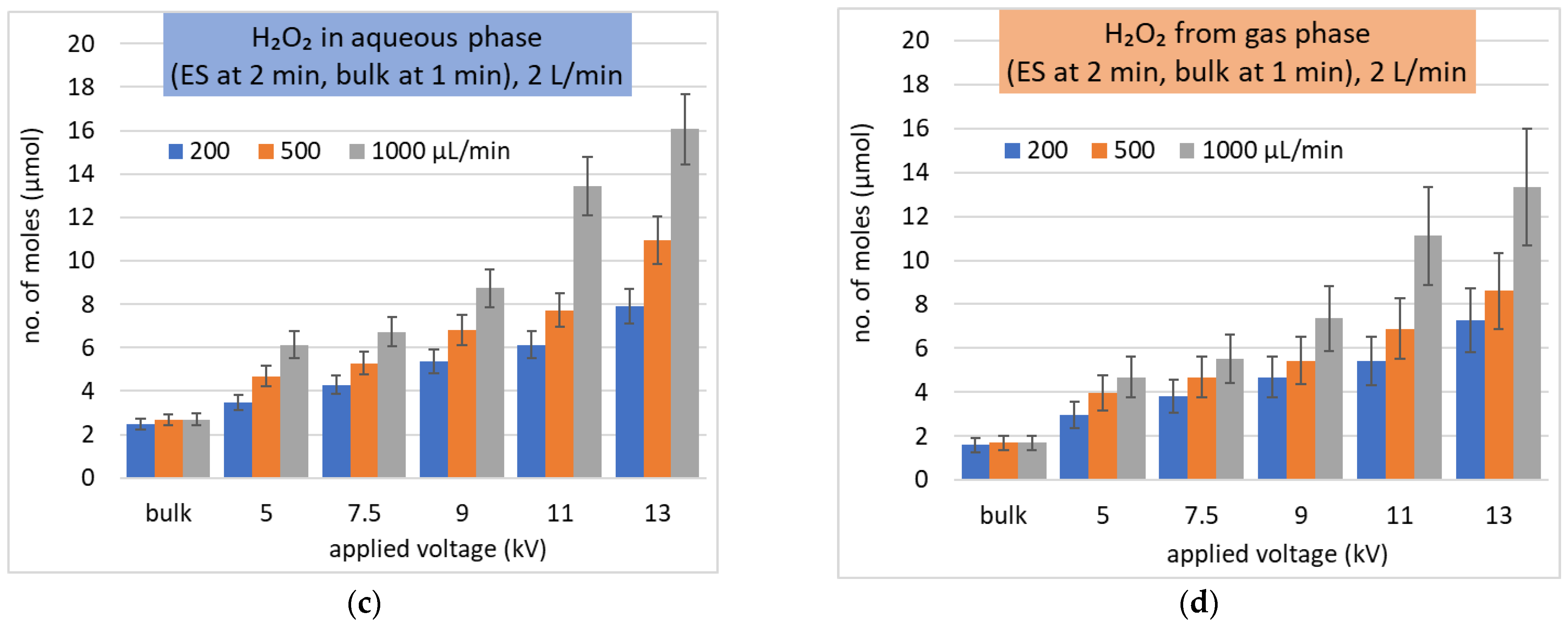
Solvation of H2O2 as the molar number of dissolved molecules in ES. (a,b) different gas flow rates (L/min) and Qw (µL/min) during 1 min treatment time; (b,c) the same gas flow rate 2 L/min and different treatment times (min) in ES and in (c) also bulk water added; (d) depleted H2O2 from the gas at the conditions of (c).
Figure 8.
Solvation of H2O2 as the molar number of dissolved molecules in ES. (a,b) different gas flow rates (L/min) and Qw (µL/min) during 1 min treatment time; (b,c) the same gas flow rate 2 L/min and different treatment times (min) in ES and in (c) also bulk water added; (d) depleted H2O2 from the gas at the conditions of (c).


Figure 9.
Saturation degree ξH2O2 of H2O2 as a function of treatment time and bulk water volume.

Figure 10.
Solvation efficiency of H2O2 at a gas flow of 1 L/min as a function of Va (kV), treatment time 1 min, at different Qw (µL/min).
Figure 10.
Solvation efficiency of H2O2 at a gas flow of 1 L/min as a function of Va (kV), treatment time 1 min, at different Qw (µL/min).

Figure 11.
Speed of the ES microdroplets measured from the HS camera images and their lifetime as a function of their diameter dk.
Figure 11.
Speed of the ES microdroplets measured from the HS camera images and their lifetime as a function of their diameter dk.

Figure 12.
Saturation degree ξO3 of O3 as a function of treatment time and the bulk water depth H.

Figure 13.
Relative contribution of the droplets with different diameters to the total volume Pv(dk) and saturation degree at the end of their lifetime ξfin(dk) as a function of droplet diameter, Va = 9 and 13 kV, Qw = 300 µL/min.
Figure 13.
Relative contribution of the droplets with different diameters to the total volume Pv(dk) and saturation degree at the end of their lifetime ξfin(dk) as a function of droplet diameter, Va = 9 and 13 kV, Qw = 300 µL/min.

Figure 14.
Effective O3 saturation degree ξeff of flying microdroplets as a function of Va (kV) at different Qw (µL/min).
Figure 14.
Effective O3 saturation degree ξeff of flying microdroplets as a function of Va (kV) at different Qw (µL/min).

Figure 15.
Comparison of O3 ξeff calculated from the size distribution histograms (Figure 5) of flying microdroplets with the measured ξO3 of bottom microdroplets of two sets of ES experiments (Qw = 100 and 500 µL/min), and O3 saturation in the corresponding bulk experiments.
Figure 15.
Comparison of O3 ξeff calculated from the size distribution histograms (Figure 5) of flying microdroplets with the measured ξO3 of bottom microdroplets of two sets of ES experiments (Qw = 100 and 500 µL/min), and O3 saturation in the corresponding bulk experiments.

Publisher’s Note: MDPI stays neutral with regard to jurisdictional claims in published maps and institutional affiliations. |
© 2021 by the authors. Licensee MDPI, Basel, Switzerland. This article is an open access article distributed under the terms and conditions of the Creative Commons Attribution (CC BY) license (http://creativecommons.org/licenses/by/4.0/).
Share and Cite
MDPI and ACS Style
Hassan, M.E.; Janda, M.; Machala, Z. Transport of Gaseous Hydrogen Peroxide and Ozone into Bulk Water vs. Electrosprayed Aerosol. Water 2021, 13, 182. https://doi.org/10.3390/w13020182
AMA Style
Hassan ME, Janda M, Machala Z. Transport of Gaseous Hydrogen Peroxide and Ozone into Bulk Water vs. Electrosprayed Aerosol. Water. 2021; 13(2):182. https://doi.org/10.3390/w13020182
Chicago/Turabian StyleHassan, Mostafa Elsayed, Mário Janda, and Zdenko Machala. 2021. "Transport of Gaseous Hydrogen Peroxide and Ozone into Bulk Water vs. Electrosprayed Aerosol" Water 13, no. 2: 182. https://doi.org/10.3390/w13020182
Note that from the first issue of 2016, this journal uses article numbers instead of page numbers. See further details here.