Improving Runoff Simulation and Forecasting with Segmenting Delay of Baseflow from Fast Surface Flow in Montane High-Vegetation-Covered Catchments

Abstract

Due to the complicated terrain conditions in montane catchments, runoff formation is fast and complicated, making accurate simulation and forecasting a significant hydrological challenge. In this study, the spatiotemporal variable source mixed runoff generation module (SVSMRG) was integrated with the long short-term memory (LSTM) method, to develop a semi-distributed model (SVSMRG)-based surface flow and baseflow segmentation (SVSMRG-SBS). Herein, the baseflow was treated as a black box and forecasted using LSTM, while the surface flow was simulated using the SVSMRG module based on hydrological response units (HRUs) constructed using eco-geomorphological units. In the case study, four typical montane catchments with different climatic conditions and high vegetation coverage, located in the topographically varying mountains of the eastern Tibetan Plateau, were selected for runoff and flood process simulations using the proposed SVSMRG-SBS model. The results showed that this model had good performance in hourly runoff and flood process simulations for montane catchments. Regarding runoff simulations, the Nash–Sutcliffe efficiency coefficient ($NSE$) and correlation coefficient ($R^2$) reached 0.8241 and 0.9097, respectively. Meanwhile, for the flood simulations, the $NSE$ ranged from 0.5923 to 0.7467, and $R^2$ ranged from 0.6669 to 0.8092. For the 1-, 3-, and 5-h baseflow forecasting with the LSTM method, it was found that model performances declined when simulating the runoff processes, wherein the $NSE$ and $R^2$ between the measured and modeled runoff decreased from 0.8216 to 0.8087 and from 0.9095 to 0.8871, respectively. Similar results were found in the flood simulations, the $NSE$ and $R^2$ values declined from 0.7414–0.5885 to 0.7429–0.5716 and from 0.8042–0.6547 to 0.7936–0.6067, respectively. This means that this new model achieved perfect performance in montane catchment runoff and flood simulation and forecasting with 1-, 3-, 5-h steps. Therefore, as it considers vegetation regulation, the SVSMRG-SBS model is expected to improve runoff and flood simulation accuracy in montane high-vegetation-covered catchments.

1. Introduction

High mountains are known as the world’s natural “water towers” as they are usually the origin of large rivers [1], providing freshwater for upstream and downstream populations. Mountains provide more than 80% of terrestrial freshwater resources while covering 24% of the total land area [2]. However, the topography, vegetation, soil, climate, and snow conditions of montane watersheds vary greatly due to the influence of altitude [3]. Thus, they are generally considered to be an unknown process in the hydrological cycle [4]. Vegetation cover is closely related to the water cycle, wherein vegetation cover type affects evapotranspiration [5], and root mode, leaf area index (LAI) [6,7], stomatal conductance [8], and interception and transpiration [9] impact runoff. Meanwhile, the macropores, formed by vegetation growth and death, animal activities, soil expansion and contraction, provide important pathways for water and solutes [10]. The cracks and channels allow rapid movement of precipitation [11], accelerate the response speed of groundwater, and replenish groundwater before the soil water reaching the field capacity. The macropores change the formation of groundwater and the proportions of different runoff components. Moreover, snow and glaciers in alpine areas appear as temporarily stored and dynamically distributed water [3,12], impacting the runoff process. Therefore, in montane high-vegetation-covered catchments, the hydrological process is complicated and unclarified, particularly the complex groundwater movement resulting in a less clear runoff formation mechanism.

Hydrological models are effective tools for studying the water cycle mechanism of basins. In recent decades, data-driven, lumped, semi-distributed, and distributed hydrological models, have been widely adopted to simulate the hydrological processes of small montane basins [13]. Data-driven models generally include neural networks (NNs) and statistical methods. Over the past two decades, the use of artificial NNs (ANNs) for runoff and flood forecasting in mountainous areas has developed rapidly [14]. Araghinejad et al. [15] presented a new performance function for NN integration and a probabilistic method based on a K-nearest neighbor regression that was applied to the flood peak forecast of the Red River in Canada and the seasonal runoff forecast of the Zayandeh-rud River in Iran to improve the accuracy of hydrological forecasting. Wu et al. [16] proposed a support vector regression (SVR) model based on artificial intelligence (AI) to predict flash floods with different lead times in montane catchments. This model had good predictive performance within one to three hours. Sezen et al. [17] compared the hydrological processes simulated by data-driven models and lumped hydrological models in a karst basin and found that the lumped conceptual hydrological model (the Genie Rural, a 4-parameter Journalier (GR4J)) was superior to ANNs, deep neural networks (DNNs), and regression tree (RT) models. However, the data-driven ANN model was slightly better than the GR4J in simulating hydrological decline in the subbasins. Nevertheless, owing to the poor consideration of spatial heterogeneity of precipitation and underlying surface as well as the demand for long-term historical observed data, lumped hydrological models have limitations regarding montane catchments [13]. In recent years, with the development of modern technologies, such as geographic information systems (GIS), remote sensing (RS), and global positioning systems (GPS), the distributed hydrological models have been employed widely in montane catchments [18]. For instance, Water Flow and Balance Simulation Model (WaSiM-ETH), a distributed hydrological model combined with meteorological observation and prediction, was used in the Lago Maggiore, an alpine watershed, to conduct flood forecasting [19]. Although the WaSiM-ETH model could determine the continuous runoff hydrographs, inherent limitations of high-resolution flood and runoff forecasting in complex mountain terrain remain existed. Moreover, high-precision meteorological data are required. A motion wave-based distributed hydrological model with surface and subsurface flow components (DHM-KWSS) has also been used to reproduce runoff processes in montane basins [20]. However, the DHM-KWSS model was unable to explain long-term runoff during the dry season. In addition, the block-wise use of TOPMODEL with the Muskingum–Cunge method (BTOPMC) was employed in the Fuji River Basin of Japan [21]. This model was integrated with the Uncertainty Quantification Python Laboratory (UQ-PyL) to determine the parameters and was only used in areas where the UQ exercises were performed. Overall, the aforementioned distributed models are deficient in depicting runoff processes, especially flood processes in mountainous areas because they do not consider complex terrain, high vegetation coverage, and snow and glacier melting. Although parameters with physical mechanisms could make the hydrological process more rational, they rely on the long-term observed data to calibrate, which is difficult to obtain for ungauged montane areas. For some cases, the parameters are difficult to fit to models [22]. Moreover, the internal mechanism of hydrology is difficult to discover for some subjective reason [23]. Nowadays, because of the simple structure and free-assumptions, it is a new way to adopt ANNs models in indistinct hydrological simulation and prediction [24,25,26]. Lee et al. [27] found that the long short-term memory (LSTM) model could be used to stochastically simulate hydrological and climatic variables as it better reproduces the variability and related structure at large time scales, as well as the core statistics of the original time domain. Compared with other NNs, the LSTM is better at using time-varying characteristics of time series data [23]. Therefore, coupling the LSTM with hydrological models is a good way to simulate and predict complex runoff and flood processes. However, these studies treated the runoff processes or flood processes as a whole using ANNs without any hydrological mechanism. At present, a large number of hydrological models can be simulated for surface flow. We expect that the baseflow with complex physical mechanisms will be replaced by black box models, and the surface flow that can be described by physical mechanisms will be simulated by hydrological models.

In this study, due to the complex runoff generation mechanisms in small montane catchments, the black box method (i.e., the LSTM) and the SVSMRG module are coupled. It has great significance for: (1) simulating and forecasting runoff or flood processes in montane catchments; (2) providing a method to simulate complex, multi-sourced runoff coupled with black box models. The aims of this study include three parts. The first one is to propose a semi-distributed model (spatiotemporal variable source mixed runoff generation module-based surface flow and baseflow segmentation (SVSMRG-SBS)) that considers complex terrain and high vegetation coverage. Specifically, surface flow is simulated according to the division of hydrological response units (HRUs), and complex baseflow is simulated by the black box method (LSTM). The second one is to apply the SVSMRG-SBS model to four montane high-vegetation-covered catchments with different climatic conditions to validate its effectiveness. The last one is to improve the accuracy of runoff and flood simulation and forecasting in montane catchments.

2. Materials and Methods

2.1. Study Regions

Mount Gongga (101°30′–102°15′ E, 29°20′–30°20′ N) is located on the southeastern edge of the Qinghai–Tibet Plateau and the middle–south section of the Mount Daxue Range [28]. Its highest peak is Mount Hengduan, with a summit of 7556 m above sea level (asl) [29]. The geological structure of Mount Gongga is extremely complex, comprising diverse landforms, dense valleys, and developed water systems. The study region, the Huangbengliugou (HBLG) catchment (101°58′–102°00′ E, 29°34′–29°36′ N), which is attached to the eastern slope of Mount Gongga, is situated in the Hailuogou (HLG) forest watershed (Figure 1) and belongs to the HLG’s primary tributary. HBLG covers 7.76 km² at elevations ranging from 2891 m to 5368 m asl and is characterized by a variety of typical vertical vegetation zone spectra [30]. The vegetation coverage is 90.72% and the main soil texture type is silty clay. The land use and soil texture types are summarized in

Table 1. Land use types.

Catchment	Type	Area (km2)	Proportion (%)
Huangbengliugou (HBLG)	Woodland	0.62	7.99
	Shrubland	2.27	29.25
	Grass	4.15	53.48
	Rock	0.72	9.28
Dayi (DY)	Woodland	179.65	65.62
	Grass	37.43	13.67
	Housing construction	7.22	2.64
	Cultivated land	49.28	18.00
	Waters	0.20	0.07
Guankou (GK)	Woodland	354.38	57.01
	Grass	159.76	25.70
	Housing construction	1.46	0.23
	Cultivated land	103.47	16.65
	Waters	0.20	0.03
	Wetland	2.34	0.38
Hanwangchang (HWC)	Woodland	168.84	42.06
	Grass	39.21	9.77
	Cultivated land	193.34	48.17

and

Table 2. Soil texture types.

Catchment	Type	Area (km2)	Proportion (%)
Huangbengliugou (HBLG)	Silty Clay	6.35	81.85
	Rock	1.41	18.15
Dayi (DY)	Loamy clay	11.8	4.31
	Sandy clay	88.75	32.42
	Clay loam	173.23	63.27
Guankou (GK)	Sandy clay	254.82	40.99
	Clay loam	147.29	23.70
	Silty loam	24.94	4.01
	Sandy loam	18.33	2.95
	Sandy clay loam	176.23	28.35
Hanwangchang (HWC)	Sandy clay	42.40	10.56
	Clay loam	124.14	30.93
	Sandy loam	14.10	3.51
	Sandy clay loam	220.75	55.00

, respectively.

HBLG is on the windward slope of the southeast monsoon and belongs to the subtropical mountainous humid monsoon climate. The annual average relative humidity is above 90% and the annual average temperature is 4.2 °C, with maximum and minimum temperatures of 23.2 °C and −14 °C, respectively, at 2947.8 m asl [31]. Due to the influence of monsoons and topography, HBLG is wet and rainy, with an average annual precipitation of 1910 mm, wherein 80% of the total amount occurs from May to October [32]. The annual average number of precipitation days reaches 261 days. Most of the rainfall intensity is low while the duration is long, wherein 33.33% of the field rainfall intensity is 1.0–1.5 mm/h, and 24.24% is 1.5 mm/h [33]. In summary, HBLG is a montane high-vegetation-covered catchment with complex underlying surfaces and large vertical changes in terrain.

In this study, an additional three montane catchments with high vegetation coverage in the Sichuan province (Figure 2) were selected to verify the effectiveness of the proposed SVSMRG-SBS model. These catchments are Dayi (DY, 103°17′–103°32′ E, 30°34′–30°44′ N), Guankou (GK, 103°41′–103°56′ E, 31°05′–31°26′ N), and Hanwangchang (HWC, 103°54′–104°11′ E, 31°27′–31°42′ N). Their corresponding land use and soil texture types are summarized in Table 1 and Table 2, respectively.

2.2. Data

The observed hourly precipitation and runoff data of HBLG were derived from the Gongga Alpine Ecosystem Observation and Research Station (GAEORS), established by the Institute of Mountain Hazards and Environment, Chinese Academy of Sciences. The Alpine Meteorological Station (101°59′ E, 29°34′ N) is located 3000 m asl on the eastern slope of Mount Gongga, and obverses hydrologic features, including precipitation, evaporation, and temperature. The precipitation data are from 2001 to 2015. Meanwhile, the runoff data were obtained from the Sanying Hydrological Station (102°00′ E, 29°34′ N) for 2001 to 2015, of which data from 2004, 2010, 2011, 2012, and 2014 are missing.

The DY precipitation data were obtained from the Wushan (103°24′ E, 30°41′ N) and Xinyuan (103°20′ E, 30°37′ N) rainfall stations. The flood event data were derived from the DY Hydrological Station (103°31′ E, 30°35′ N). The data sets were from 1980 to 2012. Moreover, the precipitation data of GK were obtained from the Baiguoping (103°52′ E, 31°20′ N) and Dabao (103°47′ E, 31°14′ N) rainfall stations, and the flood event data were obtained from the GK hydrological station (103°51′ E, 31°05′ N). These data sets cover 1968 to 2012. Finally, the HWC precipitation data were taken from the Qingping (104°07′ E, 31°33′ N) and Tianchi (104°08′ E, 31°29′ N) rainfall stations, and the flood event data were obtained from the HWC Hydrological Station (104°10′ E, 31°28′ N). These data sets cover 1994 to 2011. The time resolutions of the precipitation, runoff and flood event data sets were hourly.

The attribute data (watershed boundaries, river channels, and confluence nodes) of the four catchments were all generated using digital elevation models (DEMs). DEM data were obtained from the National Aeronautics and Space Administration (NASA, https://www.nasa.gov/) at a resolution of 12.5 m × 12.5 m in HBLG, whereas for DY, GK, and HWC were derived from the Geospatial Data Cloud (http://www.gscloud.cn/) at a resolution of 30.0 m × 30.0 m.

2.3. The Model Description

Baseflow in montane areas is largely affected by vegetation, and snow and glacier melt water, and its physical generation mechanism is intricate, making it difficult to accurately describe using current hydrological models. In this study, the baseflow was simulated using the LSTM. In addition, surface flow was simulated using the SVSMRG module. Then, a semi-distributed hydrological model (i.e., SVSMRG-SBS) for simulating and forecasting runoff processes and flood processes in montane catchments with high vegetation coverage was formed. In this model, surface flow, which includes infiltration-excess runoff, saturation-excess runoff, preferential flow, and interflow, considers the unevenness of precipitation and the underlying surface, and baseflow, which refers to the outflow from the underground reservoir, uses the LSTM without a physical mechanism. The model structure is shown in Figure 3.

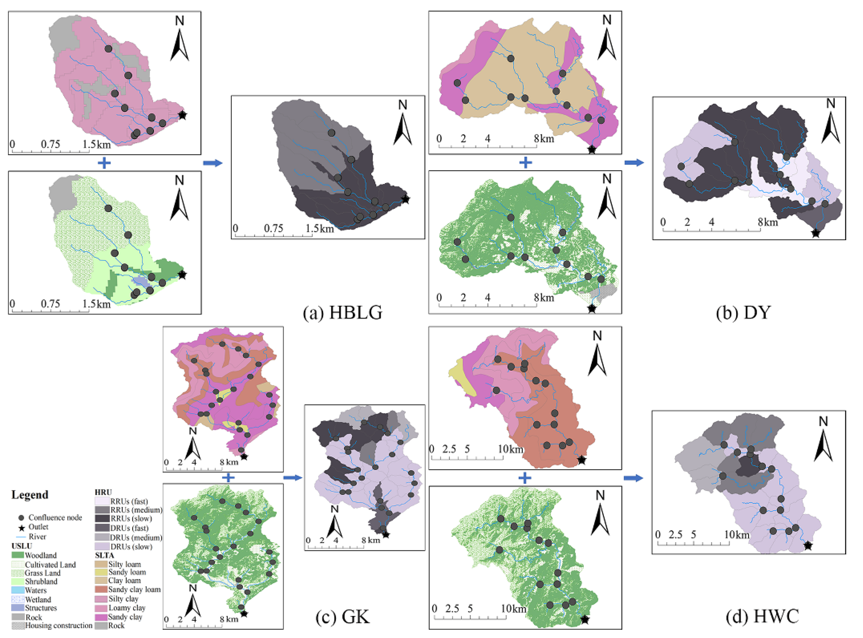
The SVSMRG-SBS model includes plane, vertical, and interval mixing. Plane mixing refers to the division of different eco-geomorphic units into different HRUs in consideration of uneven underlying surfaces, which correspond to different runoff formation mechanisms. There are four major HRU types: (1) rapid responding units (RRUs), which respond rapidly to rainfall and usually generate major infiltration-excess runoff, such as bedrock, fractured areas with bare soil, and subsidence areas; (2) disconnected rapid responding units (DRRUs), which are similar to RRUs, but lack hydraulic connection with the surrounding areas, wherein its discharge contributes less to the outlets; (3) delay responding units (DRUs), which refer to the relatively slow response speed to rainfall, and are usually grassland and woodland, wherein runoff formations are multiple components and their combinations, for instance, infiltration-excess runoff, saturation-excess runoff, and interflow; and (4) small contribution units (SCUs), which have a small contribution to runoff generation, and are usually cultivated lands. Runoff components are mainly saturation-excess runoff and interflow. These HRUs are subdivided into three types: fast, medium, and slow. Vertical mixing refers to the hydrological process in which the generation mechanisms of infiltration-excess runoff and saturation-excess runoff may be mixed in consideration of the dynamic balance of soil water. In addition, interval mixing refers to the formation of infiltration-excess runoff and saturation-excess runoff in the varying processes of instantaneous infiltration rate and infiltration capacity, soil water content, and water storage capacity. The summary of SVSMRG-SBS model characteristics is listed in

Table 3. Summary of SVSMRG-SBS model characteristics.

	Content	Description
SVSMRG-SBS model	Composition	Precipitation-runoff simulation; evapotranspiration; surface flow; interflow; groundwater; etc.
	Temporal resolution	Hourly; daily; combination of hourly and daily
	Spatial resolution	Small catchments
	Characteristic	Modular structure; a semi-distributed hydrological model with a mix of plane, vertical and interval
	Application	Simulation of the spatiotemporal transition process of infiltration-excess and saturation-excess runoff formation in small catchments under short-duration and heavy rainfall conditions

.

2.3.1. Runoff Generation Modules

Herein, the runoff generation modules include surface flow and baseflow, where surface flow considers the unevenness of precipitation and underlying surface, and baseflow is simulated using the black box model–LSTM.

(1)

Surface flow;

(a)

interception and filling.

Regarding interception:

In the intercept process, precipitation is divided into interception and net rain. Interception is related to the vegetation coverage density and intercept capacity, and is divided into summer and winter interception.

Summer interception is calculated as follows:

$$it{p}_c=(I_c^s-I_c)\times A_{HRU}\times d_s$$

(1)

$$p_{ip}=\{\begin{array}{cc}p-\frac{it{p}_c}{A_{HRU}\times d_s},& p>\frac{it{p}_c}{A_{HRU}\times d_s}\\ 0.0,& p\le \frac{it{p}_c}{A_{HRU}\times d_s}\end{array}$$

(2)

$$p_{itp}=p\times (1.0-d_s)+(p_{ip}\times d_s)$$

(3)

where $it{p}_c$ is the effective intercept capacity (mm∙m²), $I_c^s$ is the intercept capacity of the main vegetation types in summer (mm), $I_c$ is the intercept capacity of the vegetation coverage density (mm), $A_{HRU}$ is the area of the HRU (m²), $p_{ip}$ is the intercept rainfall (mm), $p$ is the precipitation (mm), $d_s$ is the vegetation coverage density in summer (-), and $p_{itp}$ is the net rainfall after interception (mm).

Meanwhile, winter interception is calculated as follows:

$$it{p}_c=(I_c^w-I_c)\times A_{HRU}\times d_w$$

(4)

$$p_{ip}=\{\begin{array}{cc}p-\frac{it{p}_c}{A_{HRU}\times d_w},& p>\frac{it{p}_c}{A_{HRU}\times d_w}\\ 0.0,& p\le \frac{it{p}_c}{A_{HRU}\times d_w}\end{array}$$

(5)

$$p_{itp}=p\times (1.0-d_w)+(p_{ip}\times d_w)$$

(6)

where $I_c^w$ is the intercept capacity of the main vegetation types in winter (mm), $d_w$ is the vegetation coverage density in winter, while the other parameters are the same as that in Equations (1)–(3).

Regarding filling:

The filling calculation is as follows:

$$PE=p_{itp}-pe{r}_{fd}\times W_{fd}$$

(7)

where $PE$ is the net rainfall (mm), $pe{r}_{fd}$ is the percentage of the basin area of depression (%), and $W_{fd}$ is the average water storage capacity of the depression (mm).

(b)

Infiltration

The model simulates the spatiotemporal transformation process of the infiltration-excess runoff and saturation-excess runoff in the HRUs in the vertical direction. Different conceptual reservoirs are used to simulate topsoil and subsoil layers, of which the topsoil is generalized into impermeable and permeable areas, and the permeable areas are separated into preferential and non-preferential flow areas. The infiltration-excess runoff formation in topsoil is simulated by the non-linear infiltration calculation method of the unsaturated zone. Meanwhile, the preferential flow areas of topsoil and subsoil are calculated based on the saturation-excess runoff formation mechanism. The preferential flow areas represent the area of proportional distribution of the infiltration-excess runoff and saturation-excess runoff areas in the HRUs. The underground reservoir is replaced by the LSTM to determine the baseflow, as detailed in Section 2.3.1–(2).

Regarding infiltration-excess runoff:

The infiltration-excess runoff formation is composed of the total net rain that falls on both pervious and impervious areas.

The net rain falling on impervious area generates surface runoff $R_{h1}$ immediately as:

$$R_{h1}=PE\times pe{r}_{ip}$$

(8)

where $pe{r}_{ip}$ is the percentage of impervious area (%).

For the net rainfall on pervious areas, if the rain intensity is stronger than the infiltration capacity, it will generate the infiltration-excess runoff $R_{h2}$ as follows:

$$R_{h2}=MAX(PE\times (1.0-pe{r}_{ip})-F_{cap},0)$$

(9)

where $F_{cap}$ is the infiltration capacity (mm).

Thus, the total infiltration-excess runoff $R_h$ is:

$$R_h=R_{h1}+R_{h2}$$

(10)

Regarding saturation-excess runoff:

The relationships between the water content of the topsoil and subsoil with soil depth and time are as follows:

$$S_{u,\max }=H_l\times {\theta }_s$$

(11)

$$S_{p,\max }=S_{u,\max }\times pe{r}_p$$

(12)

$$S_{\max }=H\times {\theta }_s$$

(13)

$$S_{u,fc}=H_l\times {\theta }_{fc}$$

(14)

$$S_{p,fc}=S_{u,fc}\times pe{r}_p$$

(15)

$$S_{fc}=H\times {\theta }_{fc}$$

(16)

$$S_{u,0}=H_l\times {\theta }_0$$

(17)

$$S_{p,0}=S_{u,0}\times pe{r}_p$$

(18)

$$S_0=H\times {\theta }_0$$

(19)

where $S_{u,\max }$ is the maximum water content of the topsoil (mm), $H_l$ is the topsoil depth (mm), ${\theta }_s$ is the saturated soil water content rate, $S_{p,\max }$ is the maximum water content of the preferential flow aquifer (mm), $pe{r}_p$ is the percentage of preferential flow area, $S_{\max }$ is the maximum soil water content (mm), $H$ is the whole soil depth (mm), $S_{u,fc}$ is the field capacity of the topsoil (mm), ${\theta }_{fc}$ is the field capacity rate, $S_{p,fc}$ is the field capacity of preferential flow aquifer (mm), $S_{fc}$ is the field capacity (mm), $S_{u,0}$ is the initial water content of topsoil (mm), ${\theta }_0$ is the initial soil water content rate, $S_{p,0}$ is the initial soil water content of the preferential flow aquifer (mm), $S_0$ is the initial soil water content (mm).

After the infiltration-excess runoff formation process, the actual infiltration amount $F$ of the topsoil is:

$$F=PE\times (1.0-pe{r}_{ip})-R_{h2}$$

(20)

The infiltration amount of the preferential flow area of the topsoil $F_p$ is:

$$F_p=pe{r}_p\times F$$

(21)

Thus, the soil water content of the preferential flow aquifer $S_p$ is:

$$S_p=MIN(S_{p,0}+F_p,S_{p,\max })$$

(22)

The first saturation-excess runoff $R_{d1}$ of the preferential flow aquifer is calculated as follows:

$$R_{d1}=MAX(0,S_{p,0}+F_p-S_{p,\max })$$

(23)

The topsoil water content $S_u$ is:

$$S_u=MIN(S_{u,0}+F,S_{u,\max })$$

(24)

Water content of the soil $S$ is calculated as follows:

$$S=MIN(S_0+F,S_{\max })$$

(25)

The subsoil water content $S_l$ is calculated as follows:

$$S_l=S-S_u$$

(26)

The second saturation-excess runoff $R_{d2}$ is:

$$R_{d2}=MAX(0,S_p+F\times pe{r}_p-S_{fc}\times pe{r}_p)$$

(27)

The total saturation-excess runoff is:

$$R_d=R_{d1}+R_{d2}$$

(28)

Regarding preferential flow:

Preferential flow $R_p$ generated in the preferential flow area of the topsoil is:

$$R_p=S_p\times k_{p1}+S_p^2\times k_{p2}$$

(29)

where $k_{p1}$ is the linear outflow coefficient of the preferential aquifer, and $k_{p2}$ is the non-linear outflow coefficient of preferential.

Regarding interflow:

Interflow $R_i$ generated by the subsoil layer is:

$$R_i=S_l\times k_{i1}+S_l^2\times k_{i2}$$

(30)

where $k_{i1}$ is the linear outflow coefficient of interflow, which includes the linear outflow coefficient of slow interflow $k_{si1}$ and the linear outflow coefficient of fast interflow $k_{fi1}$, and $k_{i2}$ is the non-linear outflow coefficient of interflow, which includes the non-linear outflow coefficient of slow interflow $k_{si2}$ and non-linear outflow coefficient of fast interflow $k_{fi2}$.

Regarding baseflow:

The outflow of the groundwater reservoir is baseflow $R_g$, which is simulated by the LSTM, as detailed in Section 2.3.1–(2).

(2)

Baseflow

The long short-term memory (LSTM) is a variant of the recurrent neural network (RNN), which is designed to avoid gradient vanishing and exploding during the process of NN training [34]. On the basis of the RNN structure, a memory block is added to the LSTM to store the information of long-term dependencies. Accordingly, the LSTM model is an effective model used for time-series and sequential data applications. Because time series forecasting has obvious characteristics of periodicity and time delay, the LSTM has been successfully applied in various forecasts, such as water table depth forecasting [35], runoff forecasting [36], and streamflow forecasting [37].

The baseflow consists of trained baseflow and predicted baseflow. Since there is no measured baseflow data, the trained baseflow is calculated via the digital filtering method called Boughton–Chapman (F4) [38] with observed or flood data series to obtain predicted baseflow in this paper.

2.3.2. Flow Routing Modules

(1)

Overland flow routing

Overland flow routing adopts a kinematic wave for description [39]. The inflow of overland is from both pervious and impervious areas. The former adopts the total amount of saturation-excess runoff and infiltration-excess runoff as the inflow, while the latter adopts net rainfall. The partial differential equation of each slope runoff field described by the kinematic wave is as follows:

$$\frac{\partial h}{\partial t}+\frac{\partial q}{\partial x}=R_d+R_h$$

(31)

where $h$ is the surface water depth (m), $q$ is the surface discharge per unit width (m²/s), $t$ is the time (s), $x$ is the distance to the downstream of the runoff field (m).

The relationship between $h$ and $q$ is as follows:

$$q=\alpha h^m$$

(32)

where $\alpha$ and m are functions representing the characteristics of the slope runoff field. See the values given by [39].

(2)

Channel flow routing

Channel flow comes from the upstream unit inflow confluence and the lateral inflow per unit channel length, described by the kinematic wave [40]. The partial differential equation is as follows:

$$\frac{\partial A}{\partial t}+\frac{\partial Q}{\partial x}=q$$

(33)

The following is the assumed relationship between river cross-sectional flow $Q$ and river cross-sectional area $A$:

$$Q=\alpha A^m$$

(34)

where $A$ is the cross-sectional area (m²), $Q$ is the cross-sectional flow (m³/s), $q$ is the lateral inflow per unit length of channel (m²/s), $t$ is the time (s), $x$ is the distance to the downstream (m), and $\alpha$ and $m$ are the kinematic wave parameters (see [39] for details).

For overland flow, as initial and boundary conditions a discharge and flow depth equal to zero is assumed. In addition, for channel flow, the initial discharge value is set as 0.028 m³/s.

2.3.3. Coupling of Baseflow and Surface Flow

In this model, the total flow $R_t$ is the sum of surface flow and baseflow, where the surface flow uses the SVSMRG module, and baseflow uses the LSTM method. $R_t$ is calculated as follows:

$$R_t=R_d+R_h+R_p+R_i+R_g$$

(35)

2.4. Evaluation Indicators of Model Calibration and Validation

Statistic metrics include $NSE$ and $R^2$, which are defined as follows:

$$NSE=1-\frac{{\displaystyle \sum _{t=1}^n{(Q_{s,t}-Q_{o,t})}^2}}{{\displaystyle \sum _{t=1}^n{(Q_{o,t}-\overline{Q_o})}^2}}$$

(36)

where $NSE$ is the Nash–Sutcliffe efficiency coefficient and the optimal value is 1, $Q_{s,t}$ and $Q_{o,t}$ are the simulated and observed runoffs at $t$ (m³/s), respectively, $\overline{Q_o}$ is the arithmetic mean observed runoff (m³/s), and n is the sample size.

$$R^2=\frac{{\displaystyle \sum _{i=1}^n{(Q_{o,t}-\overline{Q_o})}^2{(Q_{s,t}-\overline{Q_s})}^2}}{{\displaystyle \sum _{i=1}^n{(Q_{o,t}-\overline{Q_o})}^2{\displaystyle \sum _{i=1}^n{(Q_{s,t}-\overline{Q_s})}^2}}}$$

(37)

where R² is the correlation coefficient and the optimal value is 1, $\overline{Q_s}$ is the arithmetic mean of the simulated runoff (m³/s), and the other parameters are the same as in (36).

2.5. Evaluation Indicator of Sensitivity Analysis

In this study, a relative sensitivity method based on a perturbation analysis (see 3.4 for details) was employed. The formula of relative sensitivity ($RS$) is as follows:

$$RS=\frac{{\displaystyle \sum _{i=1}^{n-1}\frac{(Q_{i+1}-Q_i)/Q_b}{(P_{i+1}-P_i)/100}}}{n-1}$$

(38)

where $RS$ is the relative sensitivity ($0\le \left|RS\right|\le 0.05$, Insensitive (Ⅰ); $0.05<\left|RS\right|\le 0.20$, General sensitive (Ⅱ); $0.20<\left|RS\right|\le 1.00$, Sensitive (Ⅲ); $\left|RS\right|>1.00$, Extremely sensitive (Ⅳ)), $Q_i$ and $Q_{i+1}$ are the i-th and i+1-th simulated results, respectively (m³/s), $Q_b$ is the calibrated result (m³/s), and $P_i$ and $P_{i+1}$ are the i-th and i+1-th adjustment percentages of the parameters, respectively.

3. Results and Discussion

3.1. Model Setup

The DEM with a resolution of 12.5 m × 12.5 m was performed for hydrological analysis of the HBLG. Then, the river channels and confluence nodes were generated, and the upstream and downstream topological relationships were verified. The catchment is divided into 19 HRUs (

Table 4. Divisions of hydrological response units (HRUs).

Catchment	HRU		Area (km2)	Proportion (%)
Huangbengliugou (HBLG)	Rapid Responding Units (RRUs)	Medium	4.31	56.00
		Slow	3.45	44.00
Dayi (DY)	RRUs	Fast	39.23	14.33
		Slow	157.52	57.53
	Delay Responding Units (DRUs)	Fast	15.13	5.53
		Slow	61.90	22.61
Guankou (GK)	RRUs	Fast	0.94	0.15
		Medium	34.68	5.58
		Slow	136.87	22.02
	DRUs	Fast	39.60	6.37
		Medium	60.47	9.73
		Slow	349.05	56.15
Hanwangchang (HWC)	RRUs	Medium	114.06	28.41
		Slow	15.61	3.89
	DRUs	Medium	63.77	15.89
		Slow	207.95	51.81

), as shown in Figure 4.

3.2. Calibration and Validation

The periods of calibration and validation were from 2001 to 2007 and from 2008 to 2015, respectively. Because there were a few soil texture types in the HBLG, calibration was conducted according to the HRUs, which were derived from the shuffled complex evolution (SCE) algorithm. The key parameters were divided into six components: the responding parameters of infiltration-excess runoff, saturation-excess runoff, interflow, overland flow routing, channel flow routing, and others (

Table 5. The key parameters and ranges of the spatiotemporal variable source mixed runoff generation module-based surface flow and baseflow segmentation (SVSMRG-SBS) model.

Component	Name	Description	Range	Unit
Infiltration-excess runoff	$k_s$	Saturated hydraulic conductivity	4×10−8–6×10−6	m/s
	$H$	Soil depth	0.500–2.000	m
Saturation-excess runoff	$H_p$	Largest proportion of the area of saturation-excess runoff	0.050–1.000	-
Interflow	$k_{s2g}$	Maximum drainage coefficient from soil to underground reservoir	0.050–1.000	m/d
	$k_{si1}$	Linear outflow coefficient of slow interflow	0.000–1.000	-
	$k_{fi1}$	Linear outflow coefficient of fast interflow	0.000–1.000	-
	$k_{si2}$	Non-linear outflow coefficient of slow interflow	0.000–2.000	-
	$k_{fi2}$	Non-linear outflow coefficient of fast interflow	0.000–2.000	-
Overland flow routing	${\alpha }_{ofp}$	Kinematic parameters	Custom	-
	$m_{ofp}$		Custom
	$T_b$		4.000–20.000
	$T_p$		1.000–9.000	-
Channel flow routing	${\alpha }_{chan}$	Kinematic parameters	Custom	-
	$m_{chan}$		Custom	-
-	${\theta }_0$	Initial soil water content rate	0.010–0.500	-

). In the calibration, $NSE$ and $R^2$ values were 0.8240 and 0.9252, respectively, while in the validation, $NSE$ and R² values were 0.8241 and 0.9097, respectively. The main parameter values for calibration and validation are summarized in

Table 6. Model parameters of Huangbengliugou (HBLG), Dayi (DY), Guankou (GK), and Hanwangchang (HWC).

Parameter	HBLG	Soil Texture	DY	GK	HWC	Parameter	HBLG	Soil Texture	DY	GK	HWC
$k_s$, (m/s)	2.78 × 10−7	Sandy loam		3.18 × 10−7	1.66 × 10−6	$H$, (m)	0.122	Sandy loam		1.527	0.588
		Sandy clay loam		2.31 × 10−6	5.50 × 10−6			Sandy clay loam		0.604	1.352
		Loamy clay	8.49 × 10−8					Loamy clay	0.907
		Clay loam	9.96 × 10−8	7.72 × 10−6	1.49 × 10−7			Clay loam	0.519	0.517	0.612
		Sandy clay	1.79 × 10−7	3.27 × 10−6	1.23 × 10−6			Sandy clay	0.624	0.616	0.918
		Silty loam		4.69 × 10−6				Silty loam		0.846
Hp	0.823	Sandy loam		0.677	0.095	$k_{s2g}$, (m/d)	0.292	Sandy loam		0.851	0.377
		Sandy clay loam		0.088	0.903			Sandy clay loam		0.058	0.947
		Loamy clay	0.191					Loamy clay	0.767
		Clay loam	0.152	0.883	0.595			Clay loam	0.970	0.086	0.060
		Sandy clay	0.993	0.113	0.087			Sandy clay	0.997	0.260	0.118
		Silty loam		0.908				Silty loam		0.924
$k_{si1}$	-	Sandy loam		0.298	0.152	$k_{fi1}$	0.579	Sandy loam		0.163	0.722
		Sandy clay loam		0.485	0.070			Sandy clay loam		0.021	0.707
		Loamy clay	0.123					Loamy clay	0.703
		Clay loam	0.722	0.500	0.197			Clay loam	0.978	0.967	0.225
		Sandy clay	0.989	0.991	0.138			Sandy clay	0.984	0.143	0.871
		Silty loam		0.861				Silty loam		0.104
$k_{si2}$	-	Sandy loam		0.466	0.218	$k_{fi2}$	0.100	Sandy loam		1.712	1.595
		Sandy clay loam		0.049	0.035			Sandy clay loam		0.592	0.337
		Loamy clay	0.042					Loamy clay	0.409
		Clay loam	0.022	0.074	0.277			Clay loam	0.174	0.522	1.262
		Sandy clay	0.049	0.148	0.062			Sandy clay	0.758	1.246	1.934
		Silty loam		0.572				Silty loam		1.188
${\theta }_0$	0.299	Sandy loam		0.027	0.082	${\alpha }_{ofp}$	0.400	-	1.295	1.242	1.142
		Sandy clay loam		0.189	0.094	$m_{ofp}$	1.804	-	0.713	1.278	0.366
		Loamy clay	0.011			$T_b$	-	-	7.000	8.000	13.267
		Clay loam	0.014	0.056	0.146	$T_p$	-	-	3.000	3.000	3.681
		Sandy clay	0.016	0.205	0.098	${\alpha }_{chan}$	1.804	-	1.522	1.940	1.243
		Silty loam		0.021		$m_{chan}$	0.266	-	1.618	1.494	1.409

.

3.3. Application of the SVSMRG-SBS Model in Other Catchments

To verify the applicability of the SVSMRG-SBS model in montane catchments with high vegetation coverage, this study selected the DY, GK, and HWC catchments to construct models for hourly flood events (Figure 4). In total, there were 19 HRUs, 40 HRUs, and 25 HRUs for DY, GK, and HWC, respectively. The areas and proportions of HRUs are summarized in Table 4, and their generation is shown in Figure 4.

Regarding DY, the data series was from 1980 to 2012, wherein 1980 to 1998 was used for calibration and 1999 to 2012 was used for validation. For GK, the data series covered 1968 to 2012, wherein 1968 to 1997 was for calibration and 1998 to 2012 was for validation. For HWC, the data series covered 1994 to 2011, wherein 1994 to 2003 was used for calibration and 2004 to 2011 was used for validation. Unlike the HBLG, there were various soil texture types in these catchments. Thus, the parameters were calibrated according to the soil texture types instead of HRUs using the SCE algorithm. The calibrated model parameters are summarized in Table 6.

3.4. Sensitivity Analysis of the SVSMRG-SBS Model

An uncertainty analysis for the hydrological models was an inevitable requirement to ensure that the predicted results were meaningful [41]. Moreover, sensitivity analyses are important for determining the uncertainty of hydrological models. A sensitivity analysis could also be used to determine the key parameters and help understand the model structure. In this study, the perturbation analysis approach was used for the sensitivity analysis. Specifically, the relative optimal value of a parameter was scaled by a certain ratio for different objective functions to perform simulated results.

First, we determined the objective function. In this study, $NSE$ and $R^2$ were used as the objective functions with the same periods for both runoff and flood validation processes. Second, we determined the parameter scaling ratios. Sensitivity analyses were performed on the aforementioned 15 parameters (Table 5), wherein they were enlarged and reduced by 10%, 30%, and 50%. Finally, standardized sensitivity curves were employed to express the sensitivities of different objective functions, which considered the change rate of a parameter relative to its optimal value on the abscissa and $NSE$ or $R^2$ as the ordinate. In addition, $n$ calculated results were selected, of which the $\left|RS\right|$ value was calculated using the two adjacent calculated results, and the average value of $n-1$ was used as the $\left|RS\right|$ value. Due to space limitations, the standardized sensitivity curves of the interflow responding parameters are shown in Figure 5, and the $\left|RS\right|$ values are listed in

Table 7. Results of sensitivity analysis.

Component	Parameter	$\left|\mathit{R}\mathit{S}\right|$
		HBLG	Class	DY	Class	GK	Class	HWC	Class
Infiltration-excess runoff	$k_s$, (m/s)	0.011048	Ⅰ	0.045560	Ⅰ	0.018622	Ⅰ	0.005364	Ⅰ
	$H$, (m)	0.006538	Ⅰ	0.082515	II	10.421367	IV	0.007548	Ⅰ
Saturation-excess runoff	Hp	0.088706	II	0.000000	I	0.305498	III	0.507296	III
Interflow	$k_{s2g}$, (m/d)	0.001150	Ⅰ	0.061162	II	0.023771	I	0.012148	Ⅰ
	$k_{si1}$	-	-	0.095774	II	0.128043	II	0.028547	Ⅰ
	$k_{fi1}$	0.021598	Ⅰ	0.084709	II	0.003732	Ⅰ	0.048260	Ⅰ
	$k_{si2}$	-	-	0.001750	Ⅰ	0.021730	Ⅰ	0.037775	Ⅰ
	$k_{fi2}$	0.000048	Ⅰ	0.030997	Ⅰ	0.023556	Ⅰ	0.058604	Ⅱ
Overland flow routing	$T_b$	-	-	0.005058	Ⅰ	0.001621	Ⅰ	0.000123	Ⅰ
	Tp	-	-	0.003648	Ⅰ	0.000992	Ⅰ	0.000007	Ⅰ
	${\alpha }_{ofp}$	0.000906	Ⅰ	-	-	-	-	-	-
	$m_{ofp}$	0.008076	Ⅰ	-	-	-	-	-	-
Channel flow routing	${\alpha }_{chan}$	0.145577	Ⅱ	0.710289	III	1.010506	Ⅳ	0.537620	III
	$m_{chan}$	0.126248	Ⅱ	16.168209	IV	39.060842	Ⅳ	44.882414	IV
-	${\theta }_0$	0.019601	Ⅰ	0.000917	Ⅰ	0.019723	Ⅰ	0.048090	Ⅰ

.

Table 7 summarizes that, in general, whether it is a runoff or flood process, the responding parameters of channel flow routing are relatively sensitive, whereas the responding parameters of overland flow routing and ${\theta }_0$ are relatively insensitive. (1) Runoff process: The overall sensitivities corresponding to the parameters are low, ranging from 0.000048 to 0.145577, with the exception of H_p, ${\alpha }_{chan}$, $m_{chan}$, and other component parameters, which are insensitive. Class I accounts for 72.73% of the total parameters, and class II accounts for the remaining 27.27%. (2) Flood process: In addition to ${\alpha }_{ofp}$, $m_o{}_{fp}$, and ${\theta }_0$, each component has relatively sensitive parameters, with a variation range of 0 to 44.882414. Among all the parameters, classes I to Ⅳ account for 61.54%, 15.38%, 10.26%, and 12.82%, respectively. Regarding each component, the responding parameter of infiltration-excess runoff $k_s$ is more sensitive than $H$ for the runoff process, while the opposite behavior for flood process. This is mainly because precipitation intensity during the flood process is generally strong, and the flood process rises and falls steeply, and thus $k_s$ changes insensitively. Meanwhile, the runoff process is relatively slow, causing $k_s$ to be more sensitive. The corresponding parameter sensitivities of interflow are closely related to the soil texture types of each catchment. Regarding HBLG, the soil texture type is mainly silty clay with a dense structure. Hence, there is more interflow drainage than that of the groundwater downward recharge. Thus, the outflow coefficient is more sensitive than the drainage coefficient to the underground reservoir. The laws of the other three catchments are similar. The slow outflow coefficients of DY and GK are more sensitive than the fast outflow coefficients because the sum of the RRUs (slow) and DRUs (slow) of these two catchments is 80.14% and 78.17%, respectively, making the former more sensitive. Meanwhile, the fast outflow coefficient of HWC is more sensitive than the slow outflow coefficient. Although the sum of the RRUs (slow) and DRUs (slow) and the sum of the RRUs (fast) and DRUs (fast) are 55.70% and 44.30%, respectively, the sum of the sandy clay loam and clay loam is 85.92% as it has a dense texture and responds strongly to precipitation, causing the fast outflow coefficient to be more sensitive. The laws of standardized sensitivity curves (Figure 5) are roughly the same as the |RS| values, but the parametric sensitivities vary for distinct objective functions, which is primarily reflected on the responding parameters of interflow in the four catchments. Using DY as an example, the parametric sensitivities with $NSE$ as the objective function are: $k_{si2}$ < $k_{fi2}$ < $k_{s2g}$ < $k_{fi1}$ < $k_{si1}$, whereas when $R^2$ is the objective function, they are: $k_{si2}$ < $k_{s2g}$ < $k_{fi\mathrm{i}}$ < $k_{fi2}$ < $k_{si1}$.

In summary, the sensitive parameters of the runoff processes are $H_p$, ${\alpha }_{chan}$, and $m_{chan}$, and H, $H_p$, $k_{si1}$, $k_{fi1}$, ${\alpha }_{chan}$, and $m_{chan}$ for the flood processes. That is, there are differences in the sensitive parameters and sensitivities between the runoff and flood processes. Meanwhile, there are differences in the parametric sensitivities due to different soil texture types during the flood processes. Consequently, when using the SVSMRG-SBS model to simulate the hydrological processes, not only should the influences of different soil texture types on the parameters be considered but also the influences of different time durations on parametric sensitivities should be considered.

3.5. Runoff and Flood Simulation and Forecasting of SVSMRG-SBS Model

During the dry season (November to mid-May of the following year) in montane catchments, river discharge is mainly derived from groundwater, including glacier melting flow. During the flood period (May 16 to the end of October), river discharge is derived from groundwater and precipitation. Therefore, flow from November 1 to May 15 of the following year comes from the baseflow, whereas the flow from May 16 to October 31 comes from the sum of baseflow and surface flow in the SVSMRG-SBS model. Furthermore, based on the LSTM, a previous 24-h observed flow was trained to obtain the baseflow at the current time (t = 0) and the predicted baseflow at 1, 3, 5 h ahead of time (t = 1, t = 3, and t = 5, respectively). Regarding runoff, the flow and baseflow data series from March 1, 2001 to March 1, 2002 were trained to predict the baseflow from 2002 to 2015 in HBLG. Conversely, there was only a short data series of flood events. Then, the first 200 flood and baseflow data points were adopted for training and predicting the baseflow of the remaining years for DY, GK, and HWC. The trained baseflow was calculated via the Boughton–Chapman (F4) method, among which the filtering parameters $f_1$ and $f_2$ and iteration $N$ were set to 0.95, 0.15, and 3.00, respectively. The results are summarized in Figure 6 and

Table 8. The values of Nash–Sutcliffe Efficiency Coefficient ($NSE$) and Correlation Coefficient ($R^2$) during calibration and validation periods (t = 0, 1, 3, and 5).

Catchment	Period	NSE				R2
		t = 0	t = 1	t = 3	t = 5	t = 0	t = 1	t = 3	t = 5
Huangbengliugou (HBLG)	Calibration	0.8240	0.8199	0.8081	0.8007	0.9252	0.9214	0.9051	0.8861
	Validation	0.8241	0.8216	0.8268	0.8087	0.9097	0.9095	0.9036	0.8871
Dayi (DY)	Calibration	0.8372	0.8365	0.8312	0.8244	0.8636	0.8615	0.8538	0.8456
	Validation	0.7467	0.7414	0.7354	0.7429	0.8092	0.8042	0.7931	0.7936
Guankou (GK)	Calibration	0.7182	0.7184	0.7166	0.7208	0.7759	0.7720	0.7639	0.7589
	Validation	0.7201	0.7155	0.7116	0.7187	0.7425	0.7369	0.7285	0.7296
Hanwangchang (HWC)	Calibration	0.8292	0.8312	0.8323	0.8302	0.8687	0.8689	0.8641	0.8598
	Validation	0.5923	0.5885	0.5765	0.5716	0.6669	0.6547	0.6226	0.6067

.

For calibration, the $NSE$ and R² values reached 0.8240 and 0.9252, respectively, for the runoff simulations, and the $NSE$ values were above 0.7182 and the $R^2$ values were above 0.7759 for the flood simulations. The SVSMRG-SBS model was thus proved to be effective. For validation, the $NSE$ and $R^2$ values reached 0.8241 and 0.9097 for the runoff simulations, while the $NSE$ ranged from 0.5923 to 0.7467, and the $R^2$ ranged from 0.6669 to 0.8092 for flood simulations. For the scenario of 1, 3, and 5 h baseflow forecasting, the model performance declined when forecasting runoff processes, as is clear when the $NSE$ and $R^2$ between the measured and modeled runoff decreased from 0.8216 to 0.8087 and from 0.9095 to 0.8871, respectively. Similar to the flood simulations, the $NSE$ and $R^2$ values declined from 0.7414–0.5885 to 0.7429–0.5716 and from 0.8042–0.6547 to 0.7936–0.6067, respectively. However, this decline was slight in each catchment. When t = 5, the NSE of HWC was only 0.5716 and the $R^2$ was only 0.6067, as a result of the poor flood data series. As forecasting time increases, the data series decreases, causing the SVSMRG-SBS model performance to decrease.

Firstly, contrast the results with results using only hydrological models: Montaldo et al. [42] used the FEST04 model, a topographically based distributed hydrologic model (TDM), and a simplified version of TDM-SDM model to predict two main floods (November 1996 and June 1997) in an alpine basin—the Toce basin (area 1534 km²). The results showed that the SDM model demonstrates satisfactory simulation performance of both floods ($NSE$ = 0.91 for the 1996 event, NSE = 0.89 for the 1997 event). Moreover, $NSE$ = 0.73 for the 1996 event, NSE = 0.84 for the 1997 event of the TDM model, and $NSE$ = 0.72 for the 1996 event, $NSE$ = 0.94 for the 1997 event of the FEST04 model. Taschner et al. [43] used the enhanced TOPMODEL to simulate the “Whitsun flood” (20th May 1999–23rd May 1999) in the Bavarian alpine forelands—the Ammer watershed (area 709 km²). The results showed that the enhanced model delivers a satisfying simulation with $NSE$ = 0.89. Grillakis et al. [44] used HBV model in five mountainous basins—Zelezniki (area 104 km²), Vester (area 213.8 km²), Zminec (area 306.5 km²), Suha (area 568.9 km²), and Medvode (area 645.7 km²) to calibrate and validate past rainfall-runoff events (1st January 2004–31st November 2007). For calibration, the $NSE$ values ranged from 0.82 to 0.96, and the $R^2$ values ranged from 0.86 to 0.96. For validation, the $NSE$ values ranged from 0.47 to 0.90, and the $R^2$ values ranged from 0.58 to 0.91. Shi et al. [45] used the HBV model to predict the floods in Tangjing catchment (area 267 km²) with 50 floods occurring between 1980 and 1999 for calibration and 20 floods occurring between 2000 and 2004 for validation. The NSE values ranged from 0.697 to 0.847, 0.669 to 0.822, and 0.645 to 0.868 for the large-sized, medium-sized, and small-sized floods, respectively. The simulation results of these studies are close to our study, but some results are slightly better than ours. The reason is that the selected flood events of above studies are few and our simulation results are the average of all the flood events. Moreover, contrast the results with results using hydrological models and ANNs hybrid models: Young and Liu [46] used four models (The Hydrologic Engineering Center’s-Hydrologic Modeling System, (HEC-HMS), single ANN, Extended Auto-Regressive Moving Average (ARMAX), and HEC-HMS-ANN) to predict runoff discharge in the southern Taiwan–Sandimen basin (area 401.78 km²) with three typhon events (Bilis, Krosa, and Sinlaku). The results showed that the $NSE$ ranged from 0.412 to 0.957 of the HEC-HMS model. Meanwhile, the predicted runoff discharge of 1, 2, 4, and 6 h ranged from 0.995 to 0.850 of the single ANN, from 0.996 to 0.533 of the ARMAX model, and from 0.993 to 0.824 of the HEC-HMS-ANN. It indicated that as the forecast time increases, the simulation accuracy decreases and is in good agreement with our results. However, the HEC-HMS-ANN hybrid model simulated results are slightly better than ours. It may be due to two reasons: (1) the mean elevation of the Sandiment basin is 1262 m asl. To some extent, the underlying surface heterogeneity, vertical zonality of soil and vegetation are not as complicated as the mountainous areas—the HBLG, DY, GK, and HWC; (2) there was only three typhon events which may make for better results.

In addition, Figure 6 shows that the simulated flow is generally lower than the observed flow. This may be because the baseflow recharge is only briefly considered, and precipitation recharge is ignored in the dry season. This may be enhanced in future study.

4. Conclusions

This study analyzed hydrological processes in montane catchments with high vegetation coverage and revealed that the baseflow formation mechanism of these catchments is complex, and easily affected by factors such as topography, underlying surface, and glacial melting water, which caused inaccurate runoff and flood simulations and forecasting. Therefore, baseflow was regarded as a black box and simulated using the LSTM, and the surface flow was simulated with a hydrological mechanism according to the eco-geomorphic units. Then, a semi-distributed hydrological model (the SVSMRG-SBS model) was proposed. It provided a method to simulate complex, multi-sourced runoff coupled with black box models. The model was found to have good performance regarding runoff and flood simulations. Note that the influences of different soil texture types and time durations on parameters must be considered. Then, the predicted 1-, 3-, and 5-h baseflow for runoff and flood forecasting were performed. Our findings showed that the simulation accuracy decreased with increasing forecast time and decreasing data series.

In this model, the LSTM was used instead of the groundwater reservoir to forecast baseflow, wherein only baseflow recharge was considered in the dry season, and precipitation recharge was ignored. This resulted in lower simulation performance. Therefore, this must be further improved to complete the model. Furthermore, the SVSMRG-SBS model is suitable for simulation of the spatiotemporal transition process of infiltration-excess and saturation-excess runoff formation in small montane catchments, where the topography and landforms are diverse and runoff generation mechanisms are complex, especially in short duration and heavy rainfall conditions.

References

1. Marques, J.; Samper-Calvete, J.; Pisani, B.; Alvares, D.; Carvalho, J.M.; I Chamine, H.; Vieira, G.; Mora, C.; Borges, F.S. Evaluation of water resources in a high-mountain basin in Serra da Estrela, Central Portugal, using a semi-distributed hydrological model. Env. Earth Sci. 2010, 62, 1219–1234. [Google Scholar] [CrossRef]
2. Martín-López, B.; Leister, I.; Cruz, P.L.; Palomo, I.; Grêt-Regamey, A.; Harrison, P.A.; Lavorel, S.; Locatelli, B.; Luque, S.; Walz, A. Nature’s contributions to people in mountains: A review. PLoS ONE 2019, 14, e0217847. [Google Scholar] [CrossRef] [PubMed] [Green Version]
3. Gurtz, J.; Baltensweiler, A.; Lang, H. Spatially distributed hydrotope-based modelling of evapotranspiration and runoff in mountainous basins. Hydrol. Process. 2015, 13, 2751–2768. [Google Scholar] [CrossRef]
4. Molnár, L. Hydrology of Mountainous Areas; IAHS: Wallingford, UK, 1992; Volume 16, pp. 498–499. [Google Scholar]
5. Beaulieu, É.; Lucas, Y.; Viville, D.; Chabaux, F.; Ackerer, P.; Goddéris, Y.; Pierret, M. Hydrological and vegetation response to climate change in a forested mountainous catchment. Model. Earth Syst. Environ. 2016, 2, 1–15. [Google Scholar] [CrossRef] [Green Version]
6. Betts, R.A.; Cox, P.M.; Lee, S.E.; Woodward, F.I. Contrasting physiological and structural vegetation feedbacks in climate change simulations. Nat. Cell Biol. 1997, 387, 796–799. [Google Scholar] [CrossRef]
7. Milly, P.C.D. Sensitivity of greenhouse summer dryness to changes in plant rooting characteristics. Geophys. Res. Lett. 1997, 24, 269–271. [Google Scholar] [CrossRef]
8. Morison, J.I.L.; Gifford, R.M. Stomatal sensitivity to carbon dioxide and humidity: A comparison of two C3 and two C4 grass species. Plant Physiol. 1983, 71, 789–796. [Google Scholar] [CrossRef] [PubMed] [Green Version]
9. Leipprand, A.; Gerten, D. Global effects of doubled atmospheric CO2 content on evapotranspiration, soil moisture and runoff under potential natural vegetation. Hydrol. Sci. J. 2006, 51, 171–185. [Google Scholar] [CrossRef] [Green Version]
10. Germann, P.; Beven, K. Kinematic wave approximation to infiltration into soils with sorbing macropores. Water Resour. Res. 1985, 21, 990–996. [Google Scholar] [CrossRef]
11. Beven, K.; Germann, P. Macropores and water flow in soils. Water Resour. Res. 1982, 18, 1311–1325. [Google Scholar] [CrossRef] [Green Version]
12. Zappa, M.; Pos, F.; Strasser, U.; Warmerdam, P.; Gurtz, J. Seasonal Water Balance of an Alpine Catchment as Evaluated by Different Methods for Spatially Distributed Snowmelt Modelling. Hydrol. Res. 2003, 34, 179–202. [Google Scholar] [CrossRef]
13. Hapuarachchi, H.A.P.; Wang, Q.J.; Pagano, T.C. A review of advances in flash flood forecasting. Hydrol. Process. 2011, 25, 2771–2784. [Google Scholar] [CrossRef]
14. Fahimi, F.; Yaseen, Z.M.; El-Shafie, A. Application of soft computing based hybrid models in hydrological variables modeling: A comprehensive review. Theor. Appl. Clim. 2016, 128, 875–903. [Google Scholar] [CrossRef]
15. Araghinejad, S.; Azmi, M.; Kholghi, M. Application of artificial neural network ensembles in probabilistic hydrological forecasting. J. Hydrol. 2011, 407, 94–104. [Google Scholar] [CrossRef]
16. Wu, J.; Liu, H.; Wei, G.; Song, T.; Zhang, C.; Zhou, H. Flash Flood Forecasting Using Support Vector Regression Model in a Small Mountainous Catchment. Water 2019, 11, 1327. [Google Scholar] [CrossRef] [Green Version]
17. Sezen, C.; Bezak, N.; Bai, Y.; Šraj, M. Hydrological modelling of karst catchment using lumped conceptual and data mining models. J. Hydrol. 2019, 576, 98–110. [Google Scholar] [CrossRef]
18. Rößler, O.; Löffler, J. Analyzing Spatio-Temporal Hydrological Processes and Related Gradients to Improve Hydrological Modeling in High Mountains. Environ. Geochem. Trop. 2009, 115, 243–256. [Google Scholar] [CrossRef]
19. Jasper, K.; Gurtz, J.; Lang, H. Advanced flood forecasting in Alpine watersheds by coupling meteorological observations and forecasts with a distributed hydrological model. J. Hydrol. 2002, 267, 40–52. [Google Scholar] [CrossRef]
20. Tanaka, T.; Tachikawa, Y. Testing the applicability of a kinematic wave-based distributed hydrological model in two climatically contrasting catchments. Hydrol. Sci. J. 2015, 60, 1361–1373. [Google Scholar] [CrossRef] [Green Version]
21. Liu, L.; Zhou, L.; Li, X.; Chen, T.; Ao, T. Screening and optimizing the sensitive parameters of BTOPMC model based on UQ-PyL software: Case study of a flood event in the Fuji river basin, Japan. J. Hydrol. Eng. 2020, 25, 05020030. [Google Scholar] [CrossRef]
22. Le, H.; Lee, H.V.; Jung, S. Application of Long Short-Term Memory (LSTM) Neural Network for Flood Forecasting. Water 2019, 11, 1387. [Google Scholar] [CrossRef] [Green Version]
23. Lv, N.; Liang, X.; Chen, C.; Zhou, Y.; Li, J.; Wei, H.; Wang, H. A long Short-Term memory cyclic model with mutual information for hydrology forecasting: A Case study in the xixian basin. Adv. Water Resour. 2020, 141, 103622. [Google Scholar] [CrossRef]
24. Cigizoglu, H.K. Estimation, forecasting and extrapolation of river flows by artificial neural networks. Hydrol. Sci. J. 2003, 48, 349–361. [Google Scholar] [CrossRef]
25. Rezaeianzadeh, M.; Tabari, H.; Arabi Yazdi, A.; Isik, S.; Kalin, L. Flood flow forecasting using ANN, ANFIS and regres-sion models. Neural Comput. Appl. 2013, 25, 25–37. [Google Scholar] [CrossRef]
26. Wang, J.; Shi, P.; Jiang, P.; Hu, J.; Qu, S.; Chen, X.; Chen, Y.; Dai, Y.; Xiao, Z. Application of BP Neural Network Algorithm in Traditional Hydrological Model for Flood Forecasting. Water 2017, 9, 48. [Google Scholar] [CrossRef] [Green Version]
27. Lee, T.; Shin, J.; Kim, J.; Singh, V.P. Stochastic simulation on reproducing long-term memory of hydroclimatological variables using deep learning model. J. Hydrol. 2020, 582, 124540. [Google Scholar] [CrossRef]
28. Hu, Z.; Wang, G.; Sun, X.; Zhu, M.; Song, C.; Huang, K.; Chen, X. Spatial-Temporal Patterns of Evapotranspiration Along an Elevation Gradient on Mount Gongga, Southwest China. Water Resour. Res. 2018, 54, 4180–4192. [Google Scholar] [CrossRef]
29. Fu, X.; Feng, X.; Zhu, W.; Wang, S.; Lu, J. Total gaseous mercury concentrations in ambient air in the eastern slope of Mt. Gongga, South-Eastern fringe of the Tibetan plateau, China. Atmos. Environ. 2008, 42, 970–979. [Google Scholar] [CrossRef]
30. Sun, J.Y.; Sun, X.Y.; Hu, Z.Y.; Wang, G.X. Exploring the influence of environmental factors in partitioning evapotran-spiration along an elevation gradient on Mount Gongga, eastern edge of the Qinghai–Tibet Platea, China. J. Mt. Sci. 2020, 17, 384–396. [Google Scholar] [CrossRef]
31. Wu, Y.; Li, W.; Zhou, J.; Cao, Y. Temperature and precipitation variations at two meteorological stations on eastern slope of Gongga Mountain, SW China in the past two decades. J. Mt. Sci. 2013, 10, 370–377. [Google Scholar] [CrossRef]
32. Sun, X.Y.; Wang, G.X.; Huang, M.; Hu, Z.Y.; Song, C.L. Effect of climate change on seasonal water use efficiency in subalpine Abies fabri. J. Mt. Sci. 2017, 14, 142–157. [Google Scholar] [CrossRef]
33. Jianzhi, N.; Xinxiao, Y.; Zhiqiang, Z. Soil preferential flow in the dark coniferous forest of Gongga Mountain based on the kinetic wave model with dispersion wave (KDW preferential flow model). Acta Ecol. Sin. 2007, 27, 3541–3555. [Google Scholar] [CrossRef]
34. Hochreiter, S.; Schmidhuber, J. Long Short-Term Memory. Neural Comput. 1997, 9, 1735–1780. [Google Scholar] [CrossRef] [PubMed]
35. Zhang, J.; Zhu, Y.; Zhang, X.; Ye, M.; Yang, J. Developing a Long Short-Term Memory (LSTM) based model for predicting water table depth in agricultural areas. J. Hydrol. 2018, 561, 918–929. [Google Scholar] [CrossRef]
36. Chen, X.; Huang, J.; Han, Z.; Gao, H.; Liu, M.; Li, Z.; Liu, X.; Li, Q.; Qi, H.; Huang, Y. The importance of short lag-time in the runoff forecasting model based on long short-term memory. J. Hydrol. 2020, 589, 125359. [Google Scholar] [CrossRef]
37. Zuo, G.; Luo, J.; Wang, N.; Lian, Y.; He, X. Decomposition ensemble model based on variational mode decomposition and long short-term memory for streamflow forecasting. J. Hydrol. 2020, 585, 124776. [Google Scholar] [CrossRef]
38. Boughton, W.C. A hydrograph-based model for estimating the water yield of ungauged catchments. Inst. Eng. Aust. Natl. Conf. 1993, 14, 317–324. [Google Scholar]
39. Ma, M.; Wen, L.; Hao, S.; Zhao, G.; Zhou, M.; Liu, C.; Wang, H.; Wang, Z. A grid-based distributed hydrological model for coal mined-out area. J. Hydrol. 2020, 588, 124990. [Google Scholar] [CrossRef]
40. Govindaraju, R.S.; Kavvas, M.L.; Jones, S.E. Approximate Analytical Solutions for Overland Flows. Water Resour. Res. 1990, 26, 2903–2912. [Google Scholar] [CrossRef]
41. Ehlers, L.; Sonnenborg, T.O.; Refsgaard, J.C. Observational and predictive uncertainties for multiple variables in a spatially distributed hydrological model. Hydrol. Process. 2018, 33, 833–848. [Google Scholar] [CrossRef]
42. Montaldo, N.; Ravazzani, G.; Mancini, M. On the prediction of the Toce alpine basin floods with distributed hydrologic models. Hydrol. Process. 2007, 21, 608–621. [Google Scholar] [CrossRef]
43. Taschner, S.; Ludwig, R.; Mauser, W. Multi-scenario flood modeling in a mountain watershed using data from a NWP model, rain radar and rain gauges. Phys. Chem. Earth Part B Hydrol. Ocean. Atmos. 2001, 26, 509–515. [Google Scholar] [CrossRef]
44. Grillakis, M.G.; Tsanis, I.K.; Koutroulis, A.G. Application of the HBV hydrological model in a flash flood case in Slovenia. Nat. Hazards Earth Syst. Sci. 2010, 10, 2713–2725. [Google Scholar] [CrossRef] [Green Version]
45. Shi, W.; Li, L.; Xia, J.; Gippel, C.J. A hydrological model modified for application to flood forecasting in medium and small-scale catchments. Arab. J. Geosci. 2016, 9, 1–15. [Google Scholar] [CrossRef]
46. Young, C.-C.; Liu, W.-C. Prediction and modelling of rainfall–runoff during typhoon events using a physically-based and artificial neural network hybrid model. Hydrol. Sci. J. 2015, 60, 2102–2116. [Google Scholar] [CrossRef]
Figure 1. The Huangbengliugou (HBLG) catchment.
Water 13 00196 g001
Figure 2. The Dayi (DY), Guankou (GK), and Hanwangchang (HWC) catchments.
Water 13 00196 g002
Figure 3. Schematic diagram of the spatiotemporal variable source mixed runoff generation module-based surface flow and baseflow segmentation (SVSMRG-SBS) model structure.
Water 13 00196 g003
Figure 4. Generations of hydrological response units (HRUs).
Water 13 00196 g004
Figure 5. Standardized sensitivity curves of responding parameters of interflow. (a): Using the Nash–Sutcliffe efficiency coefficient ( N S E ) as the objective function; (b): Using the correlation coefficient ( R 2 ) as the objective function.
Water 13 00196 g005
Figure 6. Processes of simulation and forecasting (t = 0, 1, 3 and 5). (a): Calibration periods; (b): Validation periods.
Water 13 00196 g006