Toward an Efficient Uncertainty Quantification of Streamflow Predictions Using Sparse Polynomial Chaos Expansion

Abstract

Reliable hydrologic models are essential for planning, designing, and management of water resources. However, predictions by hydrological models are prone to errors due to a variety of sources of uncertainty. More accurate quantification of these uncertainties using a large number of ensembles and model runs is hampered by the high computational burden. In this study, we developed a highly efficient surrogate model constructed by sparse polynomial chaos expansion (SPCE) coupled with the least angle regression method, which enables efficient uncertainty quantifications. Polynomial chaos expansion was employed to surrogate a storage function-based hydrological model (SFM) for nine streamflow events in the Hongcheon watershed of South Korea. The efficiency of SPCE is investigated by comparing it with another surrogate model, full polynomial chaos expansion (FPCE) built by a well-known, ordinary least square regression (OLS) method. This study confirms that (1) the performance of SPCE is superior to that of FPCE because SPCE can build a more accurate surrogate model (i.e., smaller leave-one-out cross-validation error) with one-quarter the size (i.e., 500 versus 2000). (2) SPCE can sufficiently capture the uncertainty of the streamflow, which is comparable to that of SFM. (3) Sensitivity analysis attained through visual inspection and mathematical computation of the Sobol’ index has been of great success for SPCE to capture the parameter sensitivity of SFM, identifying four parameters, $\alpha$, $K_{bas}$, $P_{bas}$, and $P_{chn}$, that are most sensitive to the likelihood function, Nash-Sutcliffe efficiency. (4) The computational power of SPCE is about 200 times faster than that of SFM and about four times faster than that of FPCE. The SPCE approach builds a surrogate model quickly and robustly with a more compact experimental design compared to FPCE. Ultimately, it will benefit ensemble streamflow forecasting studies, which must provide information and alerts in real time.

1. Introduction

Hydrological models are tools that convert climate inputs into responses to numerically represent the various physical processes of a watershed [1,2,3,4,5]. These models typically include parameters embodying temporal and spatial variability of watershed characteristics that cannot be measured explicitly [2,6]. Consequently, the predictive accuracy of hydrologic models is inevitably influenced by the uncertainty of the undetermined parameters, yielding model results that are often mismatched with observations [2,7,8,9,10,11]. Therefore, quantifying and reducing uncertainties has been a major challenge for researchers in water planning and supply, sediment management, reservoir operation, and streamflow predictions [12,13,14,15,16].

Numerous techniques for addressing uncertainty have been developed in the hydrological literature, such as generalized likelihood uncertainty estimation [17], Bayesian recursive estimation [18], the Shuffled Complex Evolution Metropolis algorithm [19], the DiffeRential Evolution Adaptive Metropolis [20], dual data assimilations [21], and simultaneous optimization and data assimilation [2]. The aforementioned methods have proven to be effective in estimating the uncertainty of model parameters. However, these methods often encounter problems with excessive computational cost, which is accompanied by a huge number of iterative calls of the model simulation to attain a satisfactory estimate of the output statistics [14,22,23]. Even using the latest sampling techniques or parallel computing methods does not significantly offset this issue [24,25,26]. To fill the gap, surrogate modeling using the polynomial chaos expansion (PCE) theory has attracted much attention in the literature, as a highly efficient solution to uncertainty quantification (UQ) [13,14,27,28,29]. PCE refers to polynomial fits to the input–output relationships of original models and thus is able to provide a flexible approximation for the model behavior given a range of parameter values. PCE that can handle both Gaussian and non-Gaussian random processes is a computationally inexpensive and effective method to surrogate any model [13,30,31].

As originally proposed by Wiener [32], PCE was based on normally-distributed random variables and a Hermite polynomial, and was later extended to be applied to any statistical distribution by Xiu and Karniadakis [31]. The key to PCE effectiveness is how to estimate PCE coefficients from the response of an original model at design points in the input space [33]. Two widely used methods for optimizing the PCE coefficients are the “projection” method, which can be cast as a numerical integration problem using quadrature or sparse-grid methods, and the “regression” method, which uses least square regression to minimize the mean square error between the surrogate model outputs and original model outputs [33]. However, both methods are incompetent in optimizing a great number of PCE coefficients because of the large number of model evaluations entailed [34,35,36]. The number of PCE coefficients increases dramatically with the number of uncertain inputs and the polynomial order. This “full” PCE requires an incredibly large number of model evaluations that severely restrict the engineering applications [37].

To circumvent this problem, methods of downsizing the PCE coefficients have been proposed such as sparse collocation [38], Bayesian compressive sensing [37], and least angle regression (LAR) [39]. Among them, LAR has received attention recently because it has been proven to provide significant computational gains over original PCE. The purpose of LAR is generally to estimate only the coefficients for the important PCE basis terms and assign zero to the coefficients for the nonessential terms. LAR enables high orders of polynomials to be fit to nonlinear complex models without substantially increasing the computational cost during the construction of a surrogate model [40]. Although the effectiveness of LAR has been demonstrated, few studies have coupled LAR with PCE in order to ensure that the original model can be accurately captured by PCE with a smaller training dataset and can provide reliable predictions with higher computational efficiency in the process of quantifying the uncertainty of a hydrologic model.

The aims of this study are to examine whether sparse PCE (SPCE) captures the behavior of a hydrological model well, quantifies the uncertainty of parameters of the hydrological model, and analyzes the sensitivity of parameters to hydrologic predictions. To highlight the effectiveness and robustness of LAR, a well-known method, the ordinary least square regression (OLS), is used and compared. The paper is structured as follows. In Section 2, methodologies of PCE and uncertainty quantification for a hydrological model are presented. Section 3 introduces a general description on a target domain, a hydrological model, and a modeling configuration. The effectiveness, robustness, and scalability of the proposed approach are demonstrated and discussed in Section 4. Finally, conclusions based on a rigorous analysis are drawn in Section 5.

2. Methodology

2.1. Polynomial Chaos Expansion

Given a modeling representation $Y=\mathit{M}\left(\mathit{X}\right)$ where the input vector $\mathit{X}$ is composed of $N_X$ uncertain parameters, $Y$ is the output response of interest (e.g., simulated streamflow), and a hydrological model $\mathit{M}$ maps the input $\mathit{X}$ into output $Y$, the model response $Y$ also can be estimated from a surrogate model ${\mathit{M}}^{\mathrm{PCE}}$ consisting of a set of polynomial bases:

$$Y=\mathit{M}\left(\mathit{X}\right)\approx {\mathit{M}}^{\mathrm{PCE}}\left(\mathit{X}\right)={\displaystyle \sum }_{\mathsf{\alpha }=0}^{\infty }{\mathsf{\epsilon }}_{\mathsf{\alpha }}{\mathsf{\Psi }}_{\mathsf{\alpha }}\left(\mathit{X}\right)$$

(1)

where ${\mathsf{\Psi }}_{\mathsf{\alpha }}\left(\mathit{X}\right)$ are corresponding multivariate polynomials given as the uncertain parameters; α is a multi-index that identifies the components of the multivariate polynomials; $\epsilon$ is unknown PCE coefficients. The multivariate polynomials ${\mathsf{\Psi }}_{\mathsf{\alpha }}\left(\mathit{X}\right)$ in Equation (1) are assembled as the tensor product of univariate orthogonal polynomials ${\mathsf{\Psi }}_{{\mathsf{\alpha }}_i}^{\left(i\right)}\left(\mathit{X}\right)$ given the degree${\mathsf{\alpha }}_i$:

$${\mathsf{\Psi }}_{\mathsf{\alpha }}\left(\mathit{X}\right)={\displaystyle \prod }_{i=1}^{N_X}{\mathsf{\Psi }}_{{\mathsf{\alpha }}_i}^{\left(i\right)}\left({\mathit{X}}_i\right)$$

(2)

For computational purposes, a truncated form of the PCE can be used [33] and described as:

$$Y=\mathit{M}\left(\mathit{X}\right)\approx {\mathit{M}}^{PCE}\left(\mathit{X}\right)={\displaystyle \sum }_{\mathsf{\alpha }=0}^{N_{\mathsf{\Psi }}-1}{\mathsf{\epsilon }}_{\mathsf{\alpha }}{\mathsf{\Psi }}_{\mathsf{\alpha }}\left(\mathit{X}\right)$$

(3)

where $N_{\mathsf{\Psi }}$ is the number of PCE coefficients (i.e., the number of polynomial expansion basis terms) determined by $N_X$ and the polynomial degree $p$ as:

$$N_{\mathsf{\Psi }}=\frac{\left(N_X+p\right)!}{N_X!p!}$$

(4)

Given the set of multivariate polynomials ${\mathsf{\Psi }}_{\mathsf{\alpha }}\left(\mathit{X}\right)$, the next step is to compute the PCE coefficients$\epsilon$. In this work, ordinary least square regression (OLS) and least angle regression (LAR) methods are adopted. First, the OLS method attempts to identify the PCE coefficients that minimize the mean-square error of approximation of the model response by the surrogate model:

$$\epsilon ={\mathrm{argmin}}_{\epsilon \in {ℝ}^{N_{\mathsf{\Psi }}}}\mathbb{E}\left[{\left(\mathit{Y}-{\displaystyle \sum }_{\mathsf{\alpha }=0}^{N_{\mathsf{\Psi }}-1}{\epsilon }_{\mathsf{\alpha }}{\mathsf{\Psi }}_{\mathsf{\alpha }}\left(\mathit{X}\right)\right)}^2\right]$$

(5)

In OLS, the number of PCE coefficients that need to be estimated is $N_{\mathsf{\Psi }}$, which can be computed from Equation (4). The surrogate model constructed by OLS is hereafter called full PCE (FPCE). Given a collection (also known as experimental design), $\mathbf{𝒳}=\left\{{\mathcal{X}}^{\left(1\right)},\dots ,{\mathcal{X}}^{\left(N\right)}\right\}$consisting of $N$ sets of parameters $\mathit{X}$ and the corresponding model response $\mathbf{𝒴}=\left\{\mathit{M}\left({\mathcal{X}}^{\left(1\right)}\right),\dots ,\mathit{M}\left({\mathcal{X}}^{\left(N\right)}\right)\right\}$, the estimates of the PCE coefficients are given by:

$$\widehat{\epsilon }={\mathrm{argmin}}_{\epsilon \in {ℝ}^{N_{\mathsf{\Psi }}}}\frac{1}{N}{\displaystyle \sum }_{k=1}^N{\left({\mathcal{Y}}^{\left(k\right)}-{\displaystyle \sum }_{\mathsf{\alpha }=0}^{N_{\mathsf{\Psi }}-1}{\epsilon }_{\mathsf{\alpha }}{\mathsf{\Psi }}_{\mathsf{\alpha }}\left({\mathcal{X}}^{\left(k\right)}\right)\right)}^2$$

(6)

which is equivalent to:

$$\widehat{\epsilon }={\left({\mathit{F}}^{\mathrm{T}}\mathit{F}\right)}^{-1}{\mathit{F}}^{\mathrm{T}}\mathbf{𝒴}$$

(7)

where $\mathit{F}$ is the $N\times N_{\mathsf{\Psi }}$ information matrix whose generic term reads:

$${\mathit{F}}_{k,\mathsf{\alpha }}={\mathsf{\Psi }}_{\mathsf{\alpha }}\left({\mathcal{X}}^{\left(k\right)}\right)k=1,\dots ,N;\mathsf{\alpha }=0,\dots ,N_{\mathsf{\Psi }}-1$$

(8)

The second LAR method is an advanced regression method in solving Equation (5) where a modification for the penalty term $\lambda {||\epsilon ||}_1$ is added:

$$\epsilon ={\mathrm{argmin}}_{\epsilon \in {ℝ}^{N_{\mathsf{\Psi }}}}\mathbb{E}\left[{\left(\mathit{Y}-{\displaystyle \sum }_{\mathsf{\alpha }=0}^{N_{\mathsf{\Psi }}-1}{\epsilon }_{\mathsf{\alpha }}{\mathsf{\Psi }}_{\mathsf{\alpha }}\left(\mathit{X}\right)\right)}^2\right]+\lambda {||\epsilon ||}_1$$

(9)

where $\lambda$ is a non-negative constant; ${||\epsilon ||}_1$ is a regularization term that forces a minimization to favor the sparse solution, computed as ${||\epsilon ||}_1={\displaystyle \sum }_{\mathsf{\alpha }\in N_{\mathsf{\Psi }}}\left|{\epsilon }_{\mathsf{\alpha }}\right|$. The main difference between LAR and OLS lies in the number of PCE coefficients, which is smaller in LAR than in OLS. Specifically, LAR determines only the multivariate polynomials ${\mathsf{\Psi }}_{\mathsf{\alpha }}\left(X\right)$ that have the most impact on the model response, while discarding polynomial terms that do not. The chosen weighty PCE coefficients are estimated, while other insignificant coefficients are set to be zero. A surrogate model is then achieved based on the sparse set of PCE terms and can be delineated as Equation (10). This surrogate model is hereafter called sparse PCE (SPCE). For a detailed description of SPCE, readers can refer to Blatman and Sudret [41]. To verify the accuracy of constructed surrogate models, the leave-one-out cross-validation error ($LOO$) is commonly used.

$$Y=\mathit{M}\left(\mathit{X}\right)\approx {\mathit{M}}^{PCE}\left(\mathit{X}\right)={\displaystyle \sum }_{\mathsf{\alpha }=0}^{S_{\mathsf{\Psi }}-1}{\epsilon }_{\mathsf{\alpha }}^s{\mathsf{\Psi }}_{\mathsf{\alpha }}^s\left(\mathit{X}\right)$$

(10)

$$LOO=\frac{1}{N}{\displaystyle \sum }_{k=1}^N{\left(\frac{\mathit{M}\left({\mathcal{X}}^{\left(k\right)}\right)-{\mathit{M}}^{PCE}\left({\mathcal{X}}^{\left(k\right)}\right)}{1-{𝒽}_k}\right)}^2$$

(11)

where ${\Psi }_{\alpha }^s\left(\mathit{X}\right)=\left\{{\Psi }_0^s\left(\mathit{X}\right),\dots ,{\Psi }_{S_{\Psi }-1}^s\left(\mathit{X}\right)\right\}$ are the set of significant polynomials; ${\epsilon }_{\alpha }^s=\left\{{\epsilon }_0^s,\dots ,{\epsilon }_{S_{\Psi }-1}^s\right\}$ are the corresponding coefficients; $S_{\Psi }$ is the number of PCE terms that are retained; ${𝒽}_k$ is the $k$-th diagonal term of the matrix$\mathit{F}{\left({\mathit{F}}^T\mathit{F}\right)}^{-1}{\mathit{F}}^T$ and the information matrix $\mathit{F}$ is defined in Equation (8).

2.2. Uncertainty Quantification of a Hydrological Model

The generalized likelihood uncertainty estimation (GLUE) method [42] is chosen to quantify the uncertainty of hydrological predictions caused by unreliable parameters. The procedure of GLUE is summarized in the following for clarity, and its details can be found in Tran and Kim [14]: (1) Determine the prior probability distribution for each uncertain parameter of concern. (2) Generate random parameter sets sampled from the prior distributions. (3) Run a hydrological model for each random set to achieve a corresponding quantity of interest (e.g., streamflow). Its accuracy is then investigated based on selected likelihood functions. (4) Separate the simulated samples into non-behavioral and behavioral runs. The behavioral runs and parameter sets refer to those satisfying a predefined acceptance level. A threshold for the acceptance can be specified as an ad-hoc value of the likelihood function, determined as an optimum value that balances efficiency and accuracy [14], or used as a ratio of the total number of simulations [20]. The posterior parameter distributions and the predictive uncertainties are then drawn from the achieved behavioral sets.

3. Study Design

3.1. Study Domain and Dataset

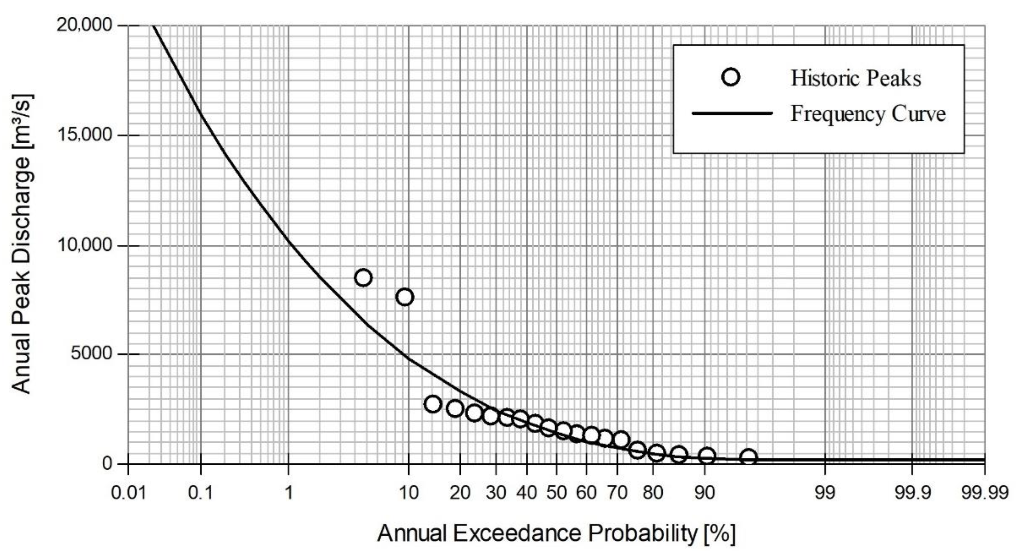
The “Hongcheon” watershed, which belongs to the Han river basin located in the central part of the Korean Peninsula, was chosen for this study (Figure 1). The area of the basin is 883 km², its mainstream length is about 60 km, and its altitude ranges from 75 to 1180 m. This study collects data for the rainy season (June to September), focusing on the uncertainty of flood predictions. Rainfall data are observed at 15 weather stations near the study area, and streamflows are observed at the outlet of the watershed, “Hongcheon” gauge station (Korea station ID = 2014650). Hourly observations of rainfall and streamflow data were downloaded from the Han River Flood Control Office (http://www.hrfco.go.kr/main.do). After inspecting the data availability within the period of 2009–2019, nine streamflow events (

Table 1. Characteristics of selected streamflow events.

Event	Time (DD/MM/YYYY)	Flow Peak (m3/s)	Flow Frequency (%)	Duration (h)
1	7–17 July 2009	2485.33	19	241
2	10–20 July 2012	416.61	86	241
3	10–17 July 2013	2264.07	28	169
4	21–27 July 2013	477.59	81	145
5	23–27 July 2015	477.60	81	97
6	29 June–9 July 2016	1460.90	52	241
7	30 June–5 July 2017	1616.14	47	121
8	9–13 July 2017	1337.97	57	97
9	27–31 August 2018	689.41	76	97

) were chosen, corresponding to various (low, middle, and high) return periods based on frequency analysis (Figure 2).

3.2. Hydrological Model

A conceptual, lumped, storage function-based hydrological model was employed, which has been adopted for streamflow prediction practice at the Han River Flood Control Office under the Ministry of Environment of Korea [43,44,45,46]. The storage function model (SFM) [47] is an event-based, lumped model that characterizes the relations of rainfall, runoff, and storage in watersheds and channels by solving the flow continuity equation. Rather than solving the full dynamic momentum equations, the SFM employs a nonlinear relation between storage and discharge for a given watershed and channel as:

$$S_{bas}\left(t\right)=K_{bas}\times Q_{bas}^{P_{bas}}\left(t\right)$$

(12)

$$S_{chn}\left(t\right)=K_{chn}\times Q_{chn}^{P_{chn}}\left(t\right)$$

(13)

where $S_{bas}\left(t\right)$ and $S_{chn}\left(t\right)$ are the storage amounts of the basin and channel at time$t$, respectively; $Q_{bas}\left(t\right)$ and $Q_{chn}\left(t\right)$ are the direct runoffs (flow rates) of the basin and channel at time $t$, respectively; $K_{bas}$ and $P_{bas}$ are the storage coefficient and exponent of the basin, while $K_{chn}$ and $P_{chn}$ are the storage coefficient and exponent of the channel.

The spatially lumped continuity equation for a given basin and channel is expressed as:

$$\frac{d{S}_{bas}\left(t\right)}{dt}=R_e\left(t-T{l}_{bas}\right)-Q_{bas}\left(t\right)$$

(14)

$$\frac{d{S}_{chn}\left(t\right)}{dt}=R_e\left(t-T{l}_{chn}\right)-Q_{chn}\left(t\right)$$

(15)

where $R_e$ is the effective rainfall, and $T{l}_{bas}$ and $T{l}_{chn}$ are time delays between the effective rainfall and the outflow of the basin and channel, respectively.

In SFM, $R_e\left(t\right)$ is estimated based on the saturated rainfall approach of Sukegawa and Kitagawa [48]. Specifically, before the accumulated rainfall depth ${{\displaystyle \sum }}^{}R\left(t\right)$ reaches the saturated rainfall $R_{sa}$, $R_e\left(t\right)$ is computed based on the primary runoff ratio ($f_1$); after ${{\displaystyle \sum }}^{}R\left(t\right)$ exceeds $R_{sa}$, $R_e\left(t\right)$ is a function of the saturated runoff ratio ($f_{sa}$):

$$R_e\left(t\right)=\{\begin{array}{c}{f}_1\times R\left(t\right) {{\displaystyle \sum }}^{}R\left(t\right)<R_{sa}\\ f_{sa}\times R\left(t\right) {{\displaystyle \sum }}^{}R\left(t\right)\ge R_{sa}\end{array}$$

(16)

The lumped rainfall depth of the basin and channel ($R\left(t\right)$) is corrected based on observed rainfall depth ($R_{obs}\left(t\right)$) and rainfall multiplication factor ($\alpha$): $R\left(t\right)=\alpha \times R_{obs}\left(t\right)$. From the brief description above, one can see that a total of 10 parameters are required to control the outflow of the watershed and implement the SFM (

Table 2. Description of the SFM parameters.

Parameter	Unit	Description	Lower Bound	Upper Bound
$\alpha$	[-]	Rainfall magnification coefficient	0	1.3
$f_1$	[-]	Primary runoff ratio	0	1
$f_{sa}$	[-]	Saturated runoff ratio	0	1
$R_{sa}$	mm	Saturated rainfall	0	300
$K_{bas}$	[-]	Basin storage-discharge coefficient	1	100
$P_{bas}$	[-]	Basin storage-discharge exponent	0	1
$T{l}_{bas}$	[h]	Time delay in watershed	0	1
$K_{chn}$	[-]	Channel storage-discharge coefficient	1	100
$P_{chn}$	[-]	Channel storage-discharge exponent	0	1
$T{l}_{chn}$	[h]	Time delay in channel	0	1

). For more detail, readers can refer to Park, Kim, Kwak, and Kim [45].

3.3. Experimental Configurations

The SPCE and FPCE models were compared by investigating the ability to construct a satisfactory surrogate model with a limited training dataset, the degree of accuracy reflecting uncertainty in streamflow prediction, and the degree of improvement in the efficiency of two surrogate models compared to the original model. The following three experiments were conducted.

The first experiment was designed to demonstrate the effectiveness of SPCE in a smaller experimental design. In the literature, the size ranges from 50 to $\mathcal{O}\left({10}^4\right)$, based on the complexity of the original model [14,49,50,51]. In this experiment, a total of 10 different sizes, $N$, from 10 to 5000 were used to build the surrogate model. A polynomial degree of 3 was used, as in previous studies [13,14,26,28,29].

Given surrogate models constructed for the optimum value of $N$ determined in the first experiment, the second experiment was conducted to quantify the uncertainty of streamflow prediction for nine rainfall events. Prior distributions for the uncertain parameters were assumed to follow the uniform distribution over a given (prior) range [14,20,42]. Latin hypercube sampling (LHS) was used due to its efficiency [26]. Regarding the cutoff threshold, we employed the ratio of the total number of simulations based on the likelihood function value to differentiate between the behavior and nonbehavior runs. Specifically, the cutoff threshold was designated as the highest 1% of Nash–Sutcliffe efficiency coefficient ($\mathrm{NSE}$) values computed using 100,000 random parameters sampled from the prior distributions [14,52].

$$\mathrm{NSE}= 1-\frac{{{\displaystyle \sum }}_{t=1}^{\mathrm{T}}{(y_t^{obs}-y_t)}^2}{{{\displaystyle \sum }}_{t=1}^{\mathrm{T}}{(y_t^{obs}-\overline{y^{obs}})}^2}$$

(17)

Here, $y_t^{obs}$ and $y_t$ are observed and simulated streamflow at time $t$, respectively, and T is the total duration of a rainfall event. The uncertainty of streamflow is then represented by calculating the ensemble interval for the NSE and Peak Error (PE) metrics, which can indicate important features of a streamflow event.

$$\mathrm{PE}= \frac{\left|y_{max}^{obs}-y_{max}\right|}{y_{max}^{obs}}\times 100$$

(18)

Here, $y_{max}^{obs}$ and $y_{max}$ are observed and simulated streamflow at the peak time of the event, respectively.

Sensitivity analysis (SA) was implemented as the third experiment to recognize the critical parameters governing model behavior and to evaluate the influence of model parameters on model outputs [14,53]. These key parameters can be identified qualitatively based on the shape of the posterior distributions obtained from GLUE, or quantitatively based on the global sensitivity analysis. The latter produces the sensitivity indices for both parameters and their interactions. Sobol’ indices [54] are employed in this experiment (Appendix A).

4. Results and Discussions

4.1. The Construction of Surrogate Models

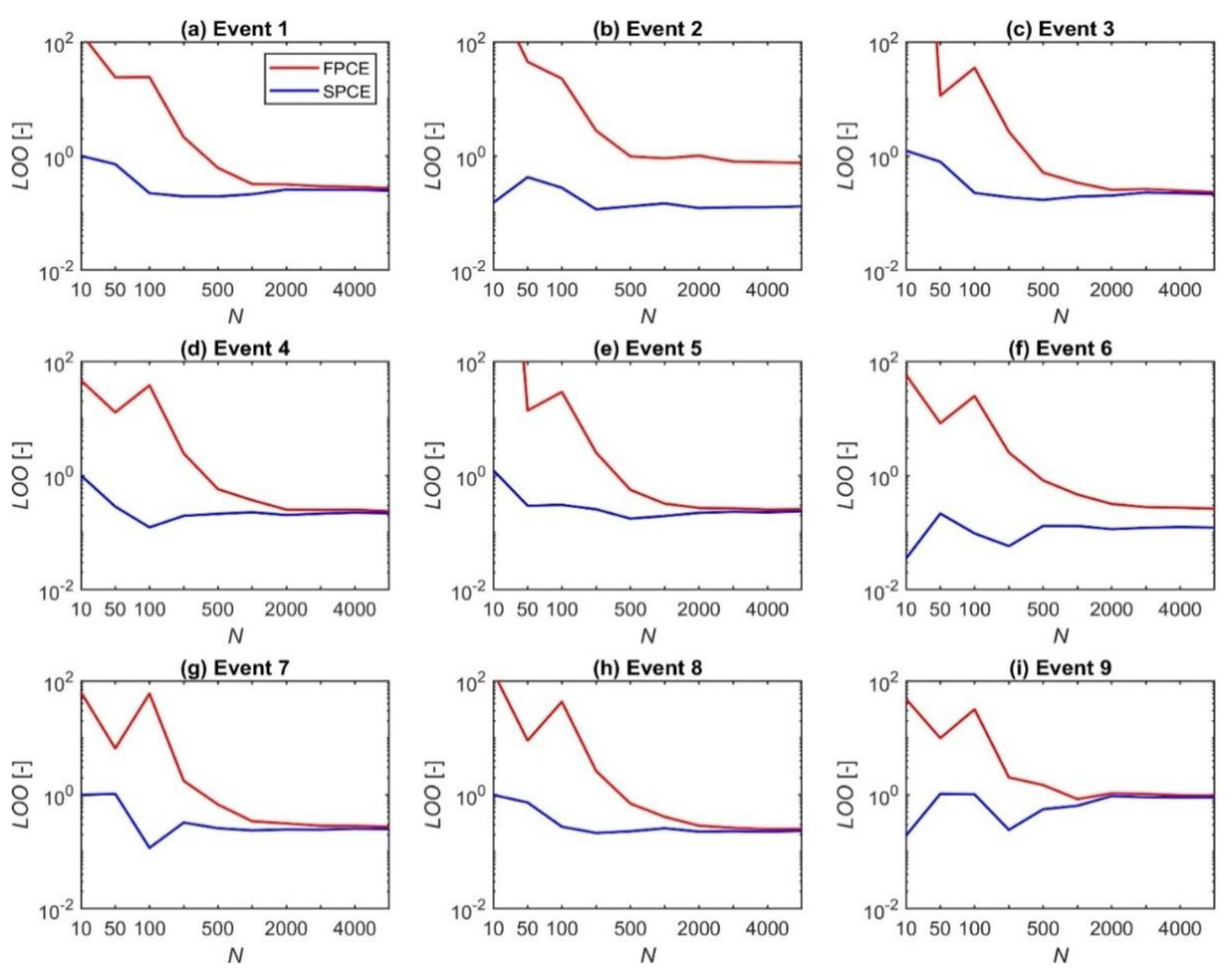
We investigate the effects of the size of the experimental design on the accuracy of surrogate models constructed by FPCE and SPCE, thereby (i) providing a guideline for choosing the appropriate size of experimental design and (ii) demonstrating the superiority of SPCE to FPCE. As described in Section 3.3, we built several surrogate models with $N$ varying between 10 and 5000 for both FPCE and SPCE. Looking at Figure 3, one can see that the $LOO$ values for all nine events decrease as the value of $N$ increases and are almost indistinguishable when $N$ reaches a certain value (about 2000 and 500 for FPCE and SPCE, respectively). In other words, if one uses a larger experimental design (greater number of samples) for training, the overall accuracy increases, but at some point the accuracy stabilizes. Visual inspection from Figure 3 confirmed that FPCE and SPCE developed with $N$ of 2000 and 500, respectively, are suitable to represent SFM. Figure 3 also reveals that SPCE outperforms FPCE in providing lesser $LOO$ values for all events. Specifically, if $N$ is less than 200, the $LOO$ values obtained using SPCE are smaller than 1, while these values for FPCE are larger, ranging from about 5 to 100. If $N$ is greater than 200, the difference of $LOO$ between two surrogates decreases by about 10%. For all events, the $LOO$ values of SPCE constructed with $N$ of 500 are equal to or even smaller than those of FPCE with $N$ of 2000. SPCE can build an efficient surrogate model with an accurate degree even if it utilizes an experimental design size that is four times smaller than that of FPCE.

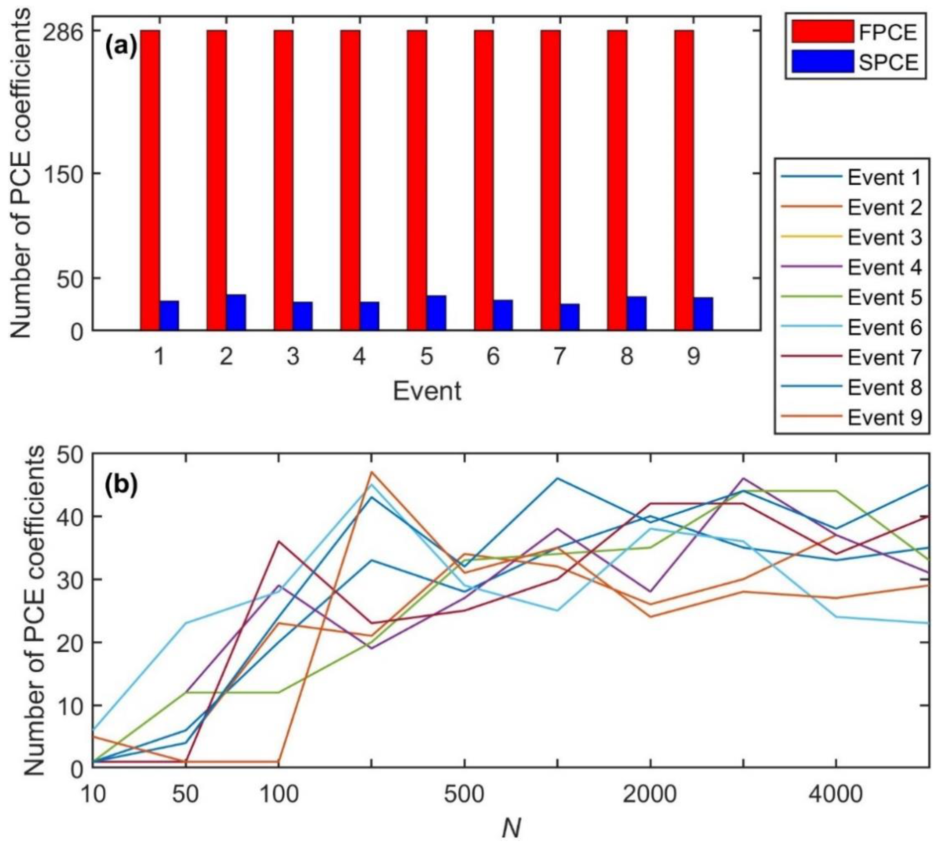
As a follow-up discussion based on the benefits of SPCE above, it can be expected that the use of this sparse approach would be more effective, especially for high-dimensional models where heavy computation is required. Since these high-dimensional models contain a large number of uncertain parameters (often greater than $\mathcal{O}\left({10}^2\right)$), the number of PCE coefficients ($N_{\Psi }$) that need to be estimated from Equation (4) are also quite large. This requires a substantial number of model evaluations, up to $N={\left(p+1\right)}^{N_X}$ [33]. This computational burden emphasizes the need for a more efficient surrogate such as SPCE to reduce the number of PCE coefficients and save computational resources. For example, for FPCE in this study, a total of 286 PCE coefficients are required for all events (computed via Equation (4) for 10 uncertain parameters and the polynomial degree of 3). For SPCE, the number of PCE coefficients ($S_{\Psi }$) used varies depending on events from 25 (Event 7) to 34 (Event 2) given $N$ of 500 (Figure 4a) and depending on $N$ (Figure 4b). $S_{\Psi }$ increases with $N$ until about 200, while it does not change much for $N$ greater than 200. $S_{\Psi }$ is always less than 50 for all events. With an appropriate value of $N$ (e.g., 500), the significant multivariate polynomials ${\Psi }_{\mathsf{\alpha }}\left(\mathit{X}\right)$ can be fully detected and it is not necessary to use a larger $N$. Therefore, the number of PCE coefficients for SPCE is about 8–11 times smaller than that of FPCE for nine events.

4.2. The Accuracy of Surrogate Models

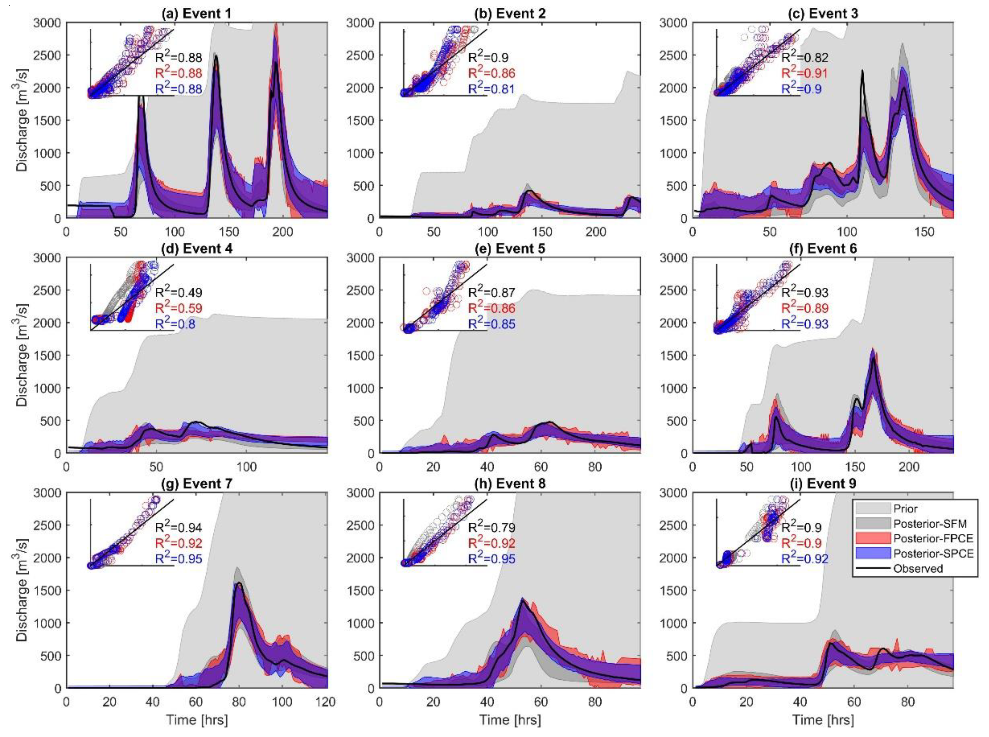
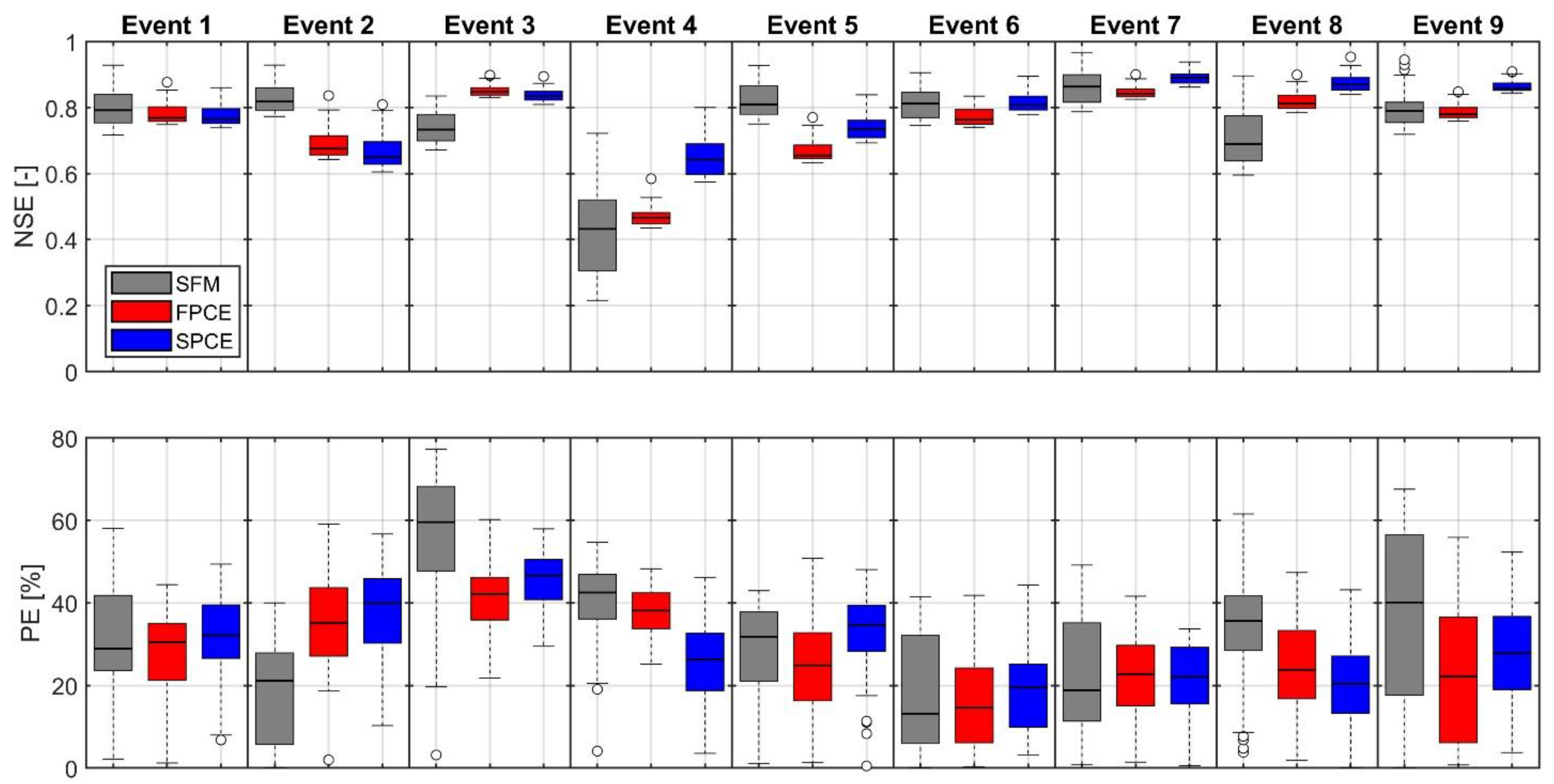
Based on the results from Section 4.1, optimum sizes of 2000 and 500 were selected for $N$ when building surrogate models for FPCE and SPCE, respectively. These surrogate models were then employed to quantify the uncertainty of hydrologic predictions through GLUE. The hydrographs of SFM, FPCE, and SPCE are presented with a 90% confidence range of 1000 behavioral (posterior) hydrographs in Figure 5. The posterior results of all three models are highly satisfactory for all nine events—their uncertainty ranges are very narrow and cover observations. The R² values for 1:1 comparisons between the ensemble mean results and observations are mostly higher than 0.8, and the R² values of two surrogate models and SFM are similar. The accuracy indices NSE and PE also confirm that both FPCE and SPCE provide a good simulation capability equivalent to SFM for diverse streamflow events with different return periods (Figure 6 and

Table 3. Mean and standard deviation (Std) for 1000 values of NSE and PE for SFM, FPCE, and SPCE for nine events.

Event	NSE [-]						PE [%]
	Mean			Std			Mean			Std
	SFM	FPCE	SPCE	SFM	FPCE	SPCE	SFM	FPCE	SPCE	SFM	FPCE	SPCE
1	0.80	0.78	0.78	0.06	0.03	0.03	30.09	27.70	31.51	14.05	10.92	10.46
2	0.83	0.69	0.67	0.04	0.04	0.05	18.90	36.19	37.61	11.84	11.66	11.65
3	0.74	0.85	0.84	0.05	0.02	0.02	56.69	42.00	45.55	15.50	7.76	6.62
4	0.43	0.47	0.65	0.13	0.03	0.06	39.52	38.17	25.00	10.07	5.75	10.59
5	0.82	0.67	0.74	0.05	0.03	0.04	28.11	25.29	32.27	11.73	12.42	10.23
6	0.81	0.77	0.81	0.05	0.03	0.03	17.26	16.10	19.29	13.81	11.82	10.41
7	0.86	0.85	0.89	0.05	0.02	0.02	21.86	22.23	21.19	13.80	10.62	9.25
8	0.72	0.82	0.87	0.09	0.03	0.02	34.54	23.79	20.39	13.91	11.13	10.88
9	0.79	0.79	0.86	0.05	0.02	0.02	37.09	22.94	27.75	20.88	16.84	12.07

). Additional comparisons between the surrogate models show that SPCE outperforms FPCE. Ensemble mean values for NSE and PE are as high as about 38% and 34% at the maximum, respectively (see Table 3 for Event 4). Additionally, the uncertainty ranges of NSE and PE for both surrogate models have smaller standard deviations (Std) than those for SFM. For example, in Event 1, the Std values of ensemble NSE for FPCE, SPCE, and SFM are 0.03, 0.03, and 0.06, respectively, while those of PE are 10.92%, 10.46%, and 14.05%, respectively (Table 3).

These ensemble results imply that the likelihood function and cutoff threshold must be carefully selected, which directly affect the prediction accuracy [14,42]. For example, since we chose NSE in this study to represent the goodness-of-fit between simulation and observation, the ensemble of NSE has a satisfactory value higher than 0.7 for most events (Figure 6). However, the peak error (PE) is relatively large, ranging from 40% (Event 6) to 78% (Event 3). That is, depending on the likelihood function preferred, one can control an outcome in streamflow prediction. If using a likelihood function that can represent the accuracy of the overall shape, peak size, time of arrival, and total flow volume of a streamflow event, it will make more informed decisions that better reflect each streamflow characteristic.

Second, to obtain more accurate ensemble results, more likelihood functions with tighter cutoff thresholds can be used. However, instead of attaining higher-accuracy ensemble results, there is a sacrifice of significantly increasing the number of random runs. For example, instead of using the 1% cutoff threshold used in this study, if we apply a cutoff threshold of 0.8 for the NSE likelihood function (this value is often considered as satisfactory [55]), the number of ensemble behavior sets decreases sharply (see the number of behavior runs for 100,000 and 10,000,000 prior runs in

Table 4. The number of behavior runs obtained through GLUE for three models (SFM, FPCE, and SPCE), based on the likelihood function of NSE with its acceptance threshold of 0.8. Column (a) and column (b) present results obtained from 100,000 and 10,000,000 random runs, respectively.

Event	(a)			(b)
	SFM	FPCE	SPCE	FPCE	SPCE
1	104	14	11	1196	1456
2	142	1	1	45	103
3	20	104	62	9520	7503
4	0	0	1	0	88
5	104	0	5	15	521
6	111	8	32	679	3306
7	181	115	219	11,147	21,771
8	36	35	84	2783	8251
9	91	13	217	1710	21,708

). The finding that there are only a very small number of ensembles signifies that random searches must be enhanced to obtain results that meet this level of accuracy. This is particularly noticeable for Event 4. With 10,000,000 random runs, SPCE could get only 88 behavior runs while FPCE could not attain even one behavior run. Additionally, an interesting aspect can be found that the acceptance rate of the behavior set is inconsistent with the size of the random run. For example, for Event 2, both FPCE and SPCE only provide one satisfactory result in 100,000 random runs, but after 10 million runs (increasing by 100 times), the number of behavior sets obtained in FPCE is 45, increasing by only 45 times. For Event 3, FPCE can provide more behavior sets than SPCE (about 0.1% vs. 0.06%). However, when increasing the number of random runs to 10,000,000 the difference in this rate is reduced (≈0.095% vs. 0.075%). Similar phenomena can be observed for other events as well. Having a behavior set of varying rates according to the number of random samples and events indicates that as many random runs as possible are needed to ensure the overall uncertainty of the parameters. However, it is still challenging to perform a large number of simulations in a high-dimensional problem due to the limitation of computational performance. The fact that a large number of iterations are required to achieve the desired accuracy justifies the use of the surrogate model. Even in a simple model like SFM, the CPU runtime required to perform 100,000 random runs was about a month, so applying the model to practical problems is unreasonable. However, for SPCE, even 10,000,000 random simulations take only a few hours to run. The surrogate model consisting of the summations of polynomials has a great advantage for Monte-Carlo type repeated simulations. We will cover the computation time of each model in more detail in Section 4.4.

4.3. The Sensitivity of Uncertain Parameters

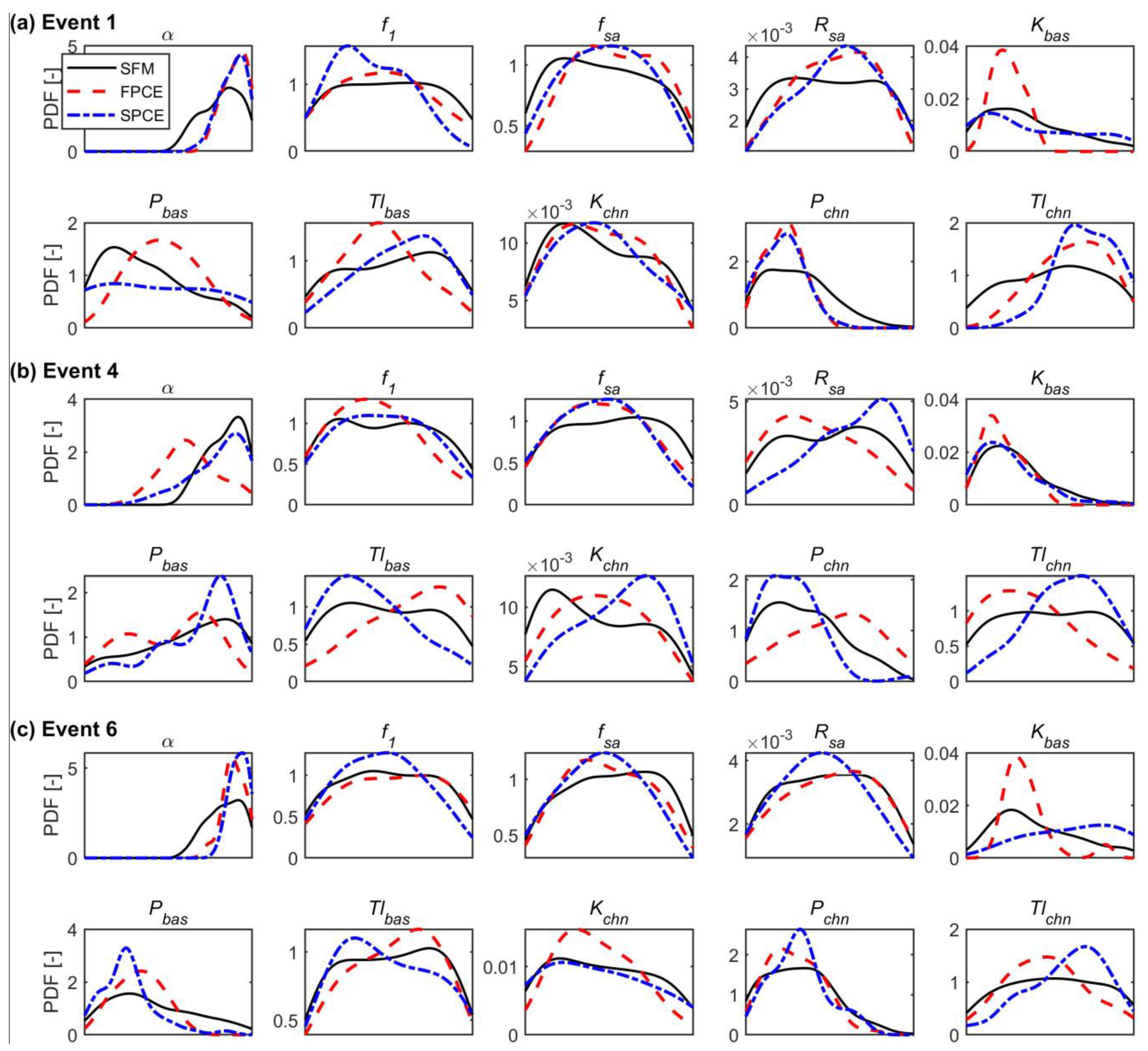
The sensitivity of each of the 10 parameters of SFM, FPCE, and SPCE was analyzed from the posterior (behavior) parameter distributions obtained by GLUE, as depicted in Figure 7. In general, parameters that have pointed distributions are relatively sensitive and identifiable, while parameters with flat-shaped distributions are insensitive and more uncertain. From a visual inspection of Figure 7, it can be seen that the parameters $\alpha$, $K_{bas}$, $P_{bas}$, and $P_{chn}$ are highly sensitive to the value of the objective function, NSE, because their distributions are relatively narrow. The remaining parameters have broader distributions, so they cannot be specified by any certain value. Additionally, marginal differences can be observed in the posterior distributions between the three models. The sensitivity results of SPCE are more analogous to those of SFM than for FPCE, especially for insensitive parameters (Figure 7). Several posterior parameter distributions obtained from FPCE have a narrower shape than those obtained from both SFM and SPCE—see $K_{bas}$, $P_{bas}$, and $T{l}_{bas}$ for Event 1; $\alpha$, $f_1$, $R_{sa}$, $K_{bas}$, $P_{bas}$, and $T{l}_{bas}$ for Event 4; and $P_{bas}$ and $T{l}_{bas}$ for Event 7.

Similar interpretations can be drawn with quantitative sensitivity analysis using the Sobol’ index (Figure 8). We confirm that the four parameters $\alpha$, $K_{bas}$, $P_{bas}$, and $P_{chn}$ are the most sensitive parameters to the likelihood function, NSE, in all events. Specifically, the sensitivities of $K_{bas}$ and $P_{bas}$ are the largest for most events, and $\alpha$ and $P_{chn}$ are the next most sensitive parameters. For events with smaller return periods (e.g., Events 4 and 5), $P_{chn}$ becomes more sensitive than the severe streamflow events. For medium to large streamflow (e.g., Events 1, 3, 7, and 9), the Sobol’ index values of the four above-mentioned sensitive parameters in SPCE are more similar to those in SFM than in FPCE (Figure 8).

Identification of principal parameters through SA can improve efficiency in the process of optimizing parameters [56]; through the analysis of the interactions, influences, and correlations among parameters, we can support a better understanding of the process mechanisms of hydrological systems [14,49,57,58]. Besides these benefits, SA helps to construct a more efficient surrogate model embracing only a subset of principal parameters. Thus, the number of PCE coefficients and the size of the experimental design could be reduced, minimizing the complexity of the model.

4.4. The Efficiency of Surrogate Models

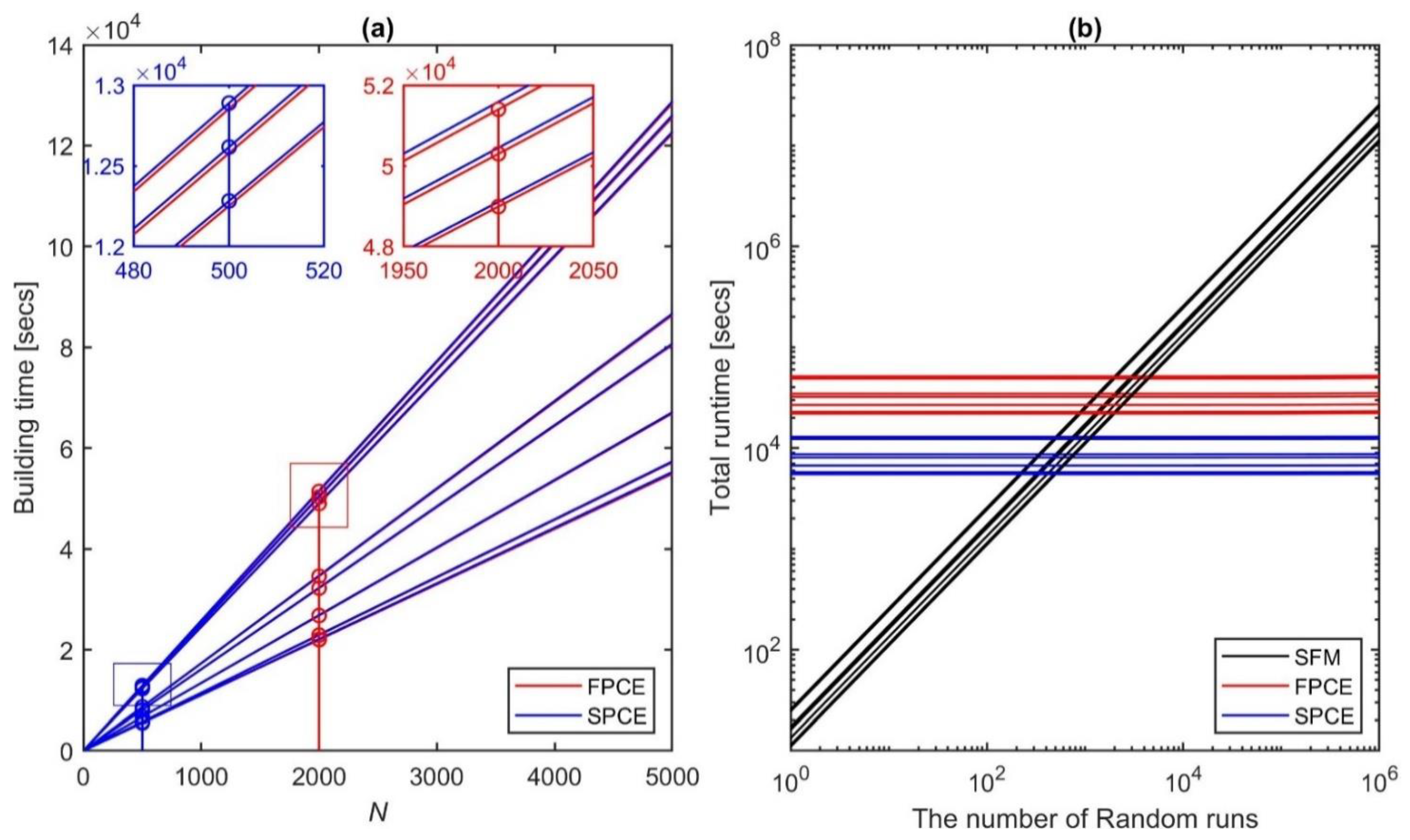
To investigate efficiency performance, all simulations were implemented under the same computer configuration (CPU Intel(R) Xeon(R) CPU E5-4660 v4 at 2.20 GHz). The total time required for executing the (surrogate) models includes building time and runtime. The building time consists of the time for evaluating the experimental design and the time for estimating the PCE coefficients; the runtime refers to the time for performing ensemble simulations (Figure 9 and

Table 5. Comparisons of the total runtime for nine streamflow events. The total runtime consists of (i) the building time and (ii) the running time. In surrogate models (FPCE and SPCE), the additional building time consists of (i-1) the time to secure the experiment design (i.e., the optimal 2000 runs for FPCE and 500 for SPCE) and (i-2) the time to compute the PCE coefficients. (ii) The latter runtime refers to the time for performing 100,000 ensemble model (SFM, FPCE, and SPCE) simulations. The unit of values is in seconds.

Event	SFM	FPCE					SPCE
	Total (ii)	Total (i) + (ii)	(i)		(ii)	Total (i) + (ii)	(i)		(ii)
			(i-1)	(i-2)			(i-1)	(i-2)
1	2,569,231	51,473	51,385	27	61	12,894	12,846	43	5
2	2,448,715	49,066	48,974	29	63	12,287	12,244	39	4
3	1,728,473	34,634	34,569	21	44	8679	8642	33	4
4	1,610,260	32,260	32,205	17	38	8078	8051	24	3
5	1,144,300	22,923	22,886	11	26	5745	5722	21	2
6	2,514,114	50,373	50,282	29	62	12,622	12,571	46	5
7	1,338,584	26,818	26,772	14	32	6716	6693	20	3
8	1,098,940	22,016	21,979	11	26	5514	5495	17	2
9	1,102,654	22,090	22,053	11	26	5531	5513	16	2

). Note that the total runtime of SFM includes only the runtime, that is, the building time is zero. Table 5 shows the comparisons of the total runtime to obtain 100,000 ensemble runs among models for nine streamflow events. Although the total runtime may vary depending on the duration of the event, SFM took 12–30 days to perform 100,000 ensemble runs, while it took 6.1–14.3 h for FPCE and only 1.5–3.6 h for SPCE to produce the same number of ensembles. In other words, the degree of efficiency improvement can be up to about 50 times for FPCE relative to SFM and up to about 200 times for SPCE. The efficiency increases for greater than 100,000 ensemble runs (Figure 9b). For example, SPCE can complete even 10,000,000 ensemble runs within 2–4 h, whereas SFM can take up to several years. When comparing the total runtime between the surrogate models, SPCE is about four times faster than FPCE. The main reason for such a difference in efficiency is that the size of the experimental design required in SPCE is smaller ($N$ = 500 vs. 2000 in FPCE). Thus, the time to secure the experimental design is about four times shorter than that of FPCE (Table 5 and Figure 9a). Additionally, with fewer polynomial terms used, the runtime of SPCE is faster than that of FPCE by about 12–14 times (see (ii) in Table 5). The ability of SPCE to perform thousands of model runs in a very short wall time enables computational problems that require a significant number of iterative calls, such as local or global optimization, data assimilation, and sensitivity analysis, to be solved efficiently [13].

5. Conclusions

This study combined SPCE with LAR to allow for efficient construction of a surrogate model and fast quantification of its uncertainty for hydrological predictions. The essence of LAR is to learn and retain only the most significant polynomial basis terms, resulting in a sparse set of PCE coefficients that could be estimated more straightforwardly. The advantages of SPCE were investigated in comparison to the performance of a surrogate model (FPCE) constructed using ordinary least square regression (OLS). Both FPCE and SPCE were developed to surrogate a storage function-based hydrological model (SFM) and then applied to quantify the uncertainties of hydrologic predictions for nine streamflow events for the ‘Hongcheon’ watershed located in South Korea. The principal outcomes highlighting the robustness and effectiveness of SPCE are summarized as follows:

• The performance of SPCE is superior to FPCE because SPCE can build a more accurate surrogate model (i.e., smaller $LOO$) with an experimental design of one-quarter the size (i.e., 500 versus 2000).
• Streamflow results obtained through GLUE demonstrated that SPCE could sufficiently capture the uncertainty of the streamflow, which is comparable to that of SFM (see high degree of agreement for NSE and PE).
• Sensitivity analysis attained through visual inspection of the posterior parameter distributions and mathematical computation of the Sobol’ index has been of great success for SPCE to capture the parameter sensitivity of SFM in middle to high flow predictions. In all models and in all events, the four parameters $\alpha$, $K_{bas}$, $P_{bas}$, and $P_{chn}$ were most sensitive to the likelihood function, NSE.
• The computational power of SPCE is about 200 times faster than SFM and about four times faster than FPCE when executing 100,000 ensemble runs. This efficiency enhancement of SPCE is particularly important when larger ensemble runs are needed.

Although this approach was applied to a lumped model with only 10 parameters, it is effective in maximizing efficiency, especially when applied to more physically based distributed models for high-dimensional problems within complex domains. The SPCE presented in this study is expected to quickly and robustly build a surrogate model with a more compact experimental design compared to FPCE. Ultimately, the approach will benefit ensemble hydrologic forecasting studies, which must provide information and alerts in real time.

References

- Wagener, T.; Wheater, H.S.; Gupta, H.V. Rainfall-Runoff Modelling in Gauged and Ungauged Catchments; Imperial College Press: London, UK, 2004. [Google Scholar]
- Vrugt, J.A.; Diks, C.G.H.; Gupta, H.V.; Bouten, W.; Verstraten, J.M. Improved treatment of uncertainty in hydrologic modeling: Combining the strengths of global optimization and data assimilation. Water Resour. Res. 2005, 41, W01017. [Google Scholar] [CrossRef]
- Kim, J.; Ivanov, V.Y. A holistic, multi-scale dynamic downscaling framework for climate impact assessments and challenges of addressing finer-scale watershed dynamics. J. Hydrol. 2015, 522, 645–660. [Google Scholar] [CrossRef] [Green Version]
- Kim, J.; Ivanov, V.Y.; Katopodes, N.D. Modeling erosion and sedimentation coupled with hydrological and overland flow processes at the watershed scale. Water Resour. Res. 2013, 49, 5134–5154. [Google Scholar] [CrossRef]
- Kim, J.; Warnock, A.; Ivanov, V.Y.; Katopodes, N.D. Coupled modeling of hydrologic and hydrodynamic processes including overland and channel flow. Adv. Water Resour. 2012, 37, 104–126. [Google Scholar] [CrossRef]
- Zhang, A.; Shi, H.; Li, T.; Fu, X. Analysis of the influence of rainfall spatial uncertainty on hydrological simulations using the bootstrap method. Atmosphere 2018, 9, 71. [Google Scholar] [CrossRef] [Green Version]
- Ajami, N.K.; Duan, Q.; Sorooshian, S. An integrated hydrologic bayesian multimodel combination framework: Confronting input, parameter, and model structural uncertainty in hydrologic prediction. Water Resour. Res. 2007, 43, W01403. [Google Scholar] [CrossRef]
- Ivanov, V.Y.; Fatichi, S.; Jenerette, G.D.; Espeleta, J.F.; Troch, P.A.; Huxman, T.E. Hysteresis of soil moisture spatial heterogeneity and the “homogenizing” effect of vegetation. Water Resour. Res. 2010, 46. [Google Scholar] [CrossRef]
- Kim, J.; Ivanov, V.Y. On the nonuniqueness of sediment yield at the catchment scale: The effects of soil antecedent conditions and surface shield. Water Resour. Res. 2014, 50, 1025–1045. [Google Scholar] [CrossRef]
- Kim, J.; Ivanov, V.Y.; Fatichi, S. Environmental stochasticity controls soil erosion variability. Sci. Rep. 2016, 6, 22065. [Google Scholar] [CrossRef] [Green Version]
- Kim, J.; Dwelle, M.C.; Kampf, S.K.; Fatichi, S.; Ivanov, V.Y. On the non-uniqueness of the hydro-geomorphic responses in a zero-order catchment with respect to soil moisture. Adv. Water Resour. 2016, 92, 73–89. [Google Scholar] [CrossRef] [Green Version]
- Benke, K.K.; Lowell, K.E.; Hamilton, A.J. Parameter uncertainty, sensitivity analysis and prediction error in a water-balance hydrological model. Math. Comput. Model. 2008, 47, 1134–1149. [Google Scholar] [CrossRef]
- Tran, V.N.; Dwelle, M.C.; Sargsyan, K.; Ivanov, V.Y.; Kim, J. A novel modeling framework for computationally efficient and accurate real-time ensemble flood forecasting with uncertainty quantification. Water Resour. Res. 2020. [Google Scholar] [CrossRef]
- Tran, V.N.; Kim, J. Quantification of predictive uncertainty with a metamodel: Toward more efficient hydrologic simulations. Stoch. Environ. Res. Risk Assess. 2019, 33, 1453–1476. [Google Scholar] [CrossRef]
- Todini, E. Role and treatment of uncertainty in real-time flood forecasting. Hydrol. Process. 2004, 18, 2743–2746. [Google Scholar] [CrossRef]
- Kim, J.; Ivanov, V.Y.; Fatichi, S. Soil erosion assessment-mind the gap. Geophys. Res. Lett. 2016, 43, 12446–12456. [Google Scholar] [CrossRef]
- Beven, K.; Binley, A. The future of distributed models: Model calibration and uncertainty prediction. Hydrol. Process. 1992, 6, 279–298. [Google Scholar] [CrossRef]
- Thiemann, M.; Trosset, M.; Gupta, H.; Sorooshian, S. Bayesian recursive parameter estimation for hydrologic models. Water Resour. Res. 2001, 37, 2521–2535. [Google Scholar] [CrossRef]
- Vrugt, J.A.; Gupta, H.V.; Bouten, W.; Sorooshian, S. A shuffled complex evolution metropolis algorithm for optimization and uncertainty assessment of hydrologic model parameters. Water Resour. Res. 2003, 39. [Google Scholar] [CrossRef] [Green Version]
- Vrugt, J.A.; ter Braak, C.J.F.; Gupta, H.V.; Robinson, B.A. Equifinality of formal (dream) and informal (glue) bayesian approaches in hydrologic modeling? Stoch. Environ. Res. Risk Assess. 2008, 23, 1011–1026. [Google Scholar] [CrossRef] [Green Version]
- Moradkhani, H.; Sorooshian, S.; Gupta, H.V.; Houser, P.R. Dual state–parameter estimation of hydrological models using ensemble kalman filter. Adv. Water Resour. 2005, 28, 135–147. [Google Scholar] [CrossRef] [Green Version]
- Liu, Y.; Gupta, H.V. Uncertainty in hydrologic modeling: Toward an integrated data assimilation framework. Water Resour. Res. 2007, 43. [Google Scholar] [CrossRef]
- Keating, E.H.; Doherty, J.; Vrugt, J.A.; Kang, Q. Optimization and uncertainty assessment of strongly nonlinear groundwater models with high parameter dimensionality. Water Resour. Res. 2010, 46. [Google Scholar] [CrossRef] [Green Version]
- Hayley, K. The present state and future application of cloud computing for numerical groundwater modeling. Ground Water 2017, 55, 678–682. [Google Scholar] [CrossRef] [PubMed]
- Vrugt, J.A.; Stauffer, P.H.; Wöhling, T.; Robinson, B.A.; Vesselinov, V.V. Inverse modeling of subsurface flow and transport properties: A review with new developments. Vadose Zone J. 2008, 7, 843. [Google Scholar] [CrossRef]
- Hu, J.; Chen, S.; Behrangi, A.; Yuan, H. Parametric uncertainty assessment in hydrological modeling using the generalized polynomial chaos expansion. J. Hydrol. 2019, 579, 124158. [Google Scholar] [CrossRef]
- Wang, S.; Ancell, B.C.; Huang, G.H.; Baetz, B.W. Improving robustness of hydrologic ensemble predictions through probabilistic pre- and post-processing in sequential data assimilation. Water Resour. Res. 2018, 54, 2129–2151. [Google Scholar] [CrossRef]
- Wang, S.; Huang, G.H.; Baetz, B.W.; Ancell, B.C. Towards robust quantification and reduction of uncertainty in hydrologic predictions: Integration of particle markov chain monte carlo and factorial polynomial chaos expansion. J. Hydrol. 2017, 548, 484–497. [Google Scholar] [CrossRef]
- Fan, Y.R.; Huang, G.H.; Baetz, B.W.; Li, Y.P.; Huang, K.; Li, Z.; Chen, X.; Xiong, L.H. Parameter uncertainty and temporal dynamics of sensitivity for hydrologic models: A hybrid sequential data assimilation and probabilistic collocation method. Environ. Model. Softw. 2016, 86, 30–49. [Google Scholar] [CrossRef] [Green Version]
- Wu, B.; Zheng, Y.; Tian, Y.; Wu, X.; Yao, Y.; Han, F.; Liu, J.; Zheng, C. Systematic assessment of the uncertainty in integrated surface water-groundwater modeling based on the probabilistic collocation method. Water Resour. Res. 2014, 50, 5848–5865. [Google Scholar] [CrossRef]
- Xiu, D.; Karniadakis, G.E. The wiener—Askey polynomial chaos for stochastic differential equations. SIAM J. Sci. Comput. 2002, 24, 619–644. [Google Scholar] [CrossRef]
- Wiener, N. The homogeneous chaos. Am. J. Math. 1938, 60, 897. [Google Scholar] [CrossRef]
- Sudret, B. Global sensitivity analysis using polynomial chaos expansions. Reliab. Eng. Syst. Saf. 2008, 93, 964–979. [Google Scholar] [CrossRef]
- Razavi, S.; Tolson, B.A.; Burn, D.H. Review of surrogate modeling in water resources. Water Resour. Res. 2012, 48. [Google Scholar] [CrossRef]
- Liu, B.; Zhang, Q.; Gielen, G.G. A gaussian process surrogate model assisted evolutionary algorithm for medium scale expensive optimization problems. IEEE Trans. Evol. Comput. 2013, 18, 180–192. [Google Scholar] [CrossRef] [Green Version]
- Blatman, G.; Sudret, B. An adaptive algorithm to build up sparse polynomial chaos expansions for stochastic finite element analysis. Probabilistic Eng. Mech. 2010, 25, 183–197. [Google Scholar] [CrossRef]
- Sargsyan, K.; Safta, C.; Najm, H.N.; Debusschere, B.J.; Ricciuto, D.; Thornton, P. Dimensionality reduction for complex models via bayesian compressive sensing. Int. J. Uncertain. Quantif. 2014, 4, 63–93. [Google Scholar] [CrossRef]
- Shi, L.; Yang, J.; Zhang, D.; Li, H. Probabilistic collocation method for unconfined flow in heterogeneous media. J. Hydrol. 2009, 365, 4–10. [Google Scholar] [CrossRef]
- Blatman, G.; Sudret, B. Sparse polynomial chaos expansions and adaptive stochastic finite elements using a regression approach. Comptes Rendus Mécanique 2008, 336, 518–523. [Google Scholar] [CrossRef]
- Zhang, J.; Zheng, Q.; Chen, D.; Wu, L.; Zeng, L. Surrogate-based bayesian inverse modeling of the hydrological system: An adaptive approach considering surrogate approximation error. Water Resour. Res. 2020, 56. [Google Scholar] [CrossRef] [Green Version]
- Blatman, G.; Sudret, B. Adaptive sparse polynomial chaos expansion based on least angle regression. J. Comput. Phys. 2011, 230, 2345–2367. [Google Scholar] [CrossRef]
- Beven, K. A manifesto for the equifinality thesis. J. Hydrol. 2006, 320, 18–36. [Google Scholar] [CrossRef] [Green Version]
- Bae, D.H.; Lee, B.J. Development of continuous rainfall-runoff model for flood forecasting on the large-scale basin. J. Korea Water Resour. Assoc. 2011, 44, 51–64. [Google Scholar] [CrossRef]
- Kim, B.; Choi, S.Y.; Han, K.Y. Integrated real-time flood forecasting and inundation analysis in small–medium streams. Water 2019, 11, 919. [Google Scholar] [CrossRef] [Green Version]
- Park, M.; Kim, D.; Kwak, J.; Kim, H. Evaluation of parameter characteristics of a storage function model. J. Hydrol. Eng. 2014, 19, 308–318. [Google Scholar] [CrossRef]
- Office, H.R.F.C. Improvement of Flood Prediction System by Applying Stochastic Technique; Ministry of Land, Transport and Maritime Affairs: Sejong, Korea, 2012.
- Kimura, T. The Flood Runoff Analysis Method by the Storage Function Model; The Public Works Research Institute, Ministry of Construction: Tokyo, Japan, 1961.
- Sukegawa, N.; Kitagawa, Y. Flood runoff model for small urban watershed with detention basins. Doboku Gakkai Ronbunshu 1992, 1992, 1–8. [Google Scholar] [CrossRef] [Green Version]
- Dwelle, M.C.; Kim, J.; Sargsyan, K.; Ivanov, V.Y. Streamflow, stomata, and soil pits: Sources of inference for complex models with fast, robust uncertainty quantification. Adv. Water Resour. 2019, 125, 13–31. [Google Scholar] [CrossRef]
- Torre, E.; Marelli, S.; Embrechts, P.; Sudret, B. Data-driven polynomial chaos expansion for machine learning regression. J. Comput. Phys. 2019, 388, 601–623. [Google Scholar] [CrossRef] [Green Version]
- Hampton, J.; Doostan, A. Compressive sampling of polynomial chaos expansions: Convergence analysis and sampling strategies. J. Comput. Phys. 2015, 280, 363–386. [Google Scholar] [CrossRef] [Green Version]
- Beven, K. Rainfall-Runoff Modelling: The Primer, 2nd ed.; Wiley-Blackwell: Oxford, UK, 2012. [Google Scholar]
- Saltelli, A. Making best use of model evaluations to compute sensitivity indices. Comput. Phys. Commun. 2002, 145, 280–297. [Google Scholar] [CrossRef]
- Sobol, I.M. Global sensitivity indices for nonlinear mathematical models and their monte carlo estimates. Math. Comput. Simul. 2001, 55, 271–280. [Google Scholar] [CrossRef]
- Moriasi, D.N.; Arnold, J.G.; Van Liew, M.W.; Bingner, R.L.; Harmel, R.D.; Veith, T.L. Model evaluation guidelines for systematic quantification of accuracy in watershed simulations. Trans. ASABE 2007, 50, 885–900. [Google Scholar] [CrossRef]
- Zhang, C.; Chu, J.; Fu, G. Sobol’s sensitivity analysis for a distributed hydrological model of yichun river basin, china. J. Hydrol. 2013, 480, 58–68. [Google Scholar] [CrossRef] [Green Version]
- Wang, H.; Gong, W.; Duan, Q.; Di, Z. Evaluation of parameter interaction effect of hydrological models using the sparse polynomial chaos (spc) method. Environ. Model. Softw. 2020, 125, 104612. [Google Scholar] [CrossRef]
- Ricciuto, D.; Sargsyan, K.; Thornton, P. The impact of parametric uncertainties on biogeochemistry in the e3sm land model. J. Adv. Model. Earth Syst. 2018, 10, 297–319. [Google Scholar] [CrossRef]
Figure 1.
The “Hongcheon” watershed belonging to Han river basin, and the locations of observed rainfall and flow gauges.
Figure 2.
Flow frequency curve for the “Hongcheon” station; historic peaks refer to annual maximum peak flows from 2000 to 2019; the flood frequency curve is fitted using the Gamma distribution.
Figure 3.
The effects of the size of experimental design () on the leave-one-out cross-validation error () in constructing surrogate models using FPCE and SPCE for nine streamflow events.
Figure 4.
(a) The number of nonzero PCE coefficients in constructing FPCE (with of 2000) and SPCE (with of 500) for nine streamflow events. (b) The effects of N on the number of PCE coefficients in SPCE for nine events.
Figure 5.
Streamflow predicted by SFM, FPCE, and SPCE for nine streamflow events. The 90% confidence bands are drawn using 1000 ensemble posterior members identified through GLUE. The scatter plots (and R2 values) represent 1:1 comparisons between the ensemble mean predictions (y-axis) and the observations (x-axis).
Figure 6.
Comparisons of accuracy metrics, NSE and PE for three models (SFM, FPCE, and SPCE) for nine streamflow events. The boxplots demonstrate the median (central mark), the 25th and 75th percentiles (the edges of the box), and the maximum and minimum (the upper and lower whiskers) except for outliers (circle symbols).
Figure 7.
Posterior distributions of 10 model parameters for three streamflow events ((a) Event 1, (b) Event 4, (c) Event 6). In each subplot, probability density functions (PDFs) are drawn by using the kernel density estimation for the 1000 behavior parameters obtained through GLUE. The range on the x-axis matches the original range values for each parameter presented in Table 2. Results for high, medium, and low return periods are only demonstrated for simplicity.
Figure 8.
Sobol’ sensitivity analysis for the 10 parameters of SFM (grey), FPCE (red), and SPCE (blue), computed for the objective function of NSE over nine streamflow events.
Figure 9.
(a) Building time of FPCE and SPCE versus the size of experimental design (N) for nine streamflow events. The building times at the optimal N = 2000 for FPCE and at N = 500 for SPCE are used for sub-figure (b) (see the stem plots and zoom-in sub-boxes in sub-figure (a)). (b) Total runtime needed for carrying out the number of model (SFM, FPCE, and SPCE) runs (from 1 to 1,000,000 on x-axis) for the nine events. Note that the intercepts of FPCE and SPCE in sub-figure (b) are equal to the building times computed in sub-figure (a), and the intercepts of SFM are zero.