The Evaluation of the Accuracy of Interpolation Methods in Crafting Maps of Physical and Hydro-Physical Soil Properties

Abstract

The goal of this study was the spatial processing and showcasing selected soil properties (available water capacity, total organic carbon content and the content of clay fraction <0.001 mm) in the Nitra River Basin (Slovakia) via the usage and the subsequent evaluation of the quality of applied interpolation methods (Spline, inverse distance weighting (IDW), Topo to Raster). The results showed the possibilities of “conversion” of point information obtained by field research as well as research in the laboratory into a spatial expression, thus providing at least relevant estimation of the soil properties even in localities not directly covered by soil sampling. Based on the evaluation and mutual comparison of the accuracy of the used interpolation methods (by using the so-called cross-validation and trust criteria), the most favorable results were achieved by the Spline method in the GRASS GIS environment, and in the ArcGIS environment. When comparing the measured and estimated values of given soil properties at control points, the interpolated values classified as very accurate up to accurate prevailed in the verification dataset. Qualitatively less favorable (but still acceptable) were the results obtained with Topo to Raster (ArcGIS) interpolation method. On the contrary, the Spline method in the ArcGIS environment turned out to be the least accurate. We assume that this is most likely not only a consequence of insufficient density of points (resources), but also an inappropriate implementation of the method into the ArcGIS environment.

1. Introduction

Rapid development of mathematical methods in various fields of knowledge and practical applications is one of the defining characteristics of modern times. Geo-statistical and geo-spatial methods are currently being used and applied in diverse scientific disciplines. Their potential lies in the swift availability of real-time spatial data, which is essential for the functioning of many industries. With the progress in the field of technology we can distribute spatial data via various software applications and layers of internet security. Over the course of last several years the amount of spatial data that the human society deals with on a daily basis has increased exponentially. New technologies for remote or terrestrial data collection, including photogrammetry or laser scanning, create a wealth of data with a certain geographical dimension. This has stimulated the development of geographic information systems aimed at storing, managing, analyzing, visualizing and making the data available to the general public.

Geographic information systems (GIS) are not limited to the field of geography per se [1], but have found broad application in agriculture [2,3,4,5], forestry [6,7], pedology [8], ecology [9], environmental studies [10,11,12,13], botany, biology, landscape planning [14], land consolidation projects [15] and nature conservation. The interconnection of GIS with other diverse scientific disciplines is necessary in the development of methodological procedures and terminology for working with spatial soil data [16].

In soil science, the applicability of GIS consists of a set of methods and means for collecting, storing, retrieving, transforming, analyzing and displaying the spatial data regarding soils from the soil continuum pertaining to their defined position within a given coordinate system, their attributive properties and their relationships to other objects occupying that same space. At present, there are several options and methodological procedures for the processing, treatment and subsequent web distribution of soil properties in the format of a map output. The soil properties are mostly determined on the basis of field sampling using soil pits and augers and the subsequent laboratory analyzes [17,18]. The accumulated data are tied to a sampling point, determined by the spatial coordinates (X, Y, Z). The result is point data of individual characteristics of soils.

A comprehensive soil survey of agricultural land took place in Slovakia (former Czechoslovakia) from 1961 up to 1970. Following the “point” information obtained by the survey, the maps of so-called evaluated (bonitated) soil-ecological units (ESEU) (in original “bonitované pôdno—ekologické jednotky“—acronym BPEJ) were elaborated at the scale 1:5000 in the 70s of the 20th century [19]. Currently, the information on the individual ESEU parameters within agricultural land in Slovakia is freely available in the soil portal of the Research Institute of Soil Science and Soil Protection in Bratislava, Slovakia [20]. The maps were accompanied by brochures with an explanation on the five-digit code by which every ESEU was specified. The system was later updated to a seven-digit code [21]. The first two digits stand for one of eleven categories of climatic regions, while the third and fourth digit specify one of one hundred main soil units. The main soil unit is formed by an aggregate of genetic soil types, sub-types, soil-forming substrates, soil texture and soil depth, degree of hydromorphism and relief of the area [22]. The fifth and sixth digits stand for the combination of slope gradient and aspect and combination of soil skeleton content and soil depth, respectively. The seventh digit specifies one of five categories of soil texture [21]. Of the available physical, hydro-physical and chemical soil properties observed during the survey, only the soil types according to soil texture (based on Novák’s classification adapted from the Kachinski system [23,24,25]) were “projected” into mapping and included in ESEUs. However, the informative value of those datasets is decreasing, as updates are elaborated only in terms of the definition of agricultural land (by drawing possible changes in the forest boundary) and slope conditions processed by geodetic activity in the landscaping process [25,26]. Knowledge on the soil properties changing over space and time is crucial for the development of various human activities. Therefore, the soil sampling and mapping is an essential part of the soil research. However, these activities are time consuming and often require special sampling and laboratory equipment and considerable financial resources. The possibility of sampling fewer sites in the field and interpolating the values of studied properties between the sampling sites is in many cases an unnecessary compromise. However, it should be mentioned that the resulting accuracy of mapping and estimation of spatial means of an environmental variable will usually be increased by dispersing the sample locations so that they cover the study area as uniformly as possible [27].

Data processing in GIS is closely linked with interpolation methods which provide a spatial estimation from point data either regularly or irregularly distributed over a given landscape segment. There is currently a wide range of interpolation algorithms [28,29,30]. Each of these algorithms is characterized by specific properties that determine its advantages or disadvantages and, of course, what is necessary, its field of application. In the case of the GRASS GIS environment, the RST algorithm (regularized spline with tension) is very often used. RST is a specific approximation, resp. interpolation function of two variables, which at the points of the points of the discrete input point field, determined by the coordinates X and Y (node points), acquires functional values close (approximation), resp. identical (interpolation) to the scalar values assigned to these points. In GRASS GIS, this function is used to calculate scalar values in the cell centers of the generated raster representing the surface produced [31].

Interpolation in the framework of understanding of GIS technology is a workflow that converts discrete spatial point information into continuous spatial information based on the assumption of spatial autocorrelation. While the usage of interpolation methods to express the shape of topography (digital terrain model) belongs among the key processes in water erosion modeling [32,33,34], its usage in other areas of soil science is less abundant e.g., [35,36,37]. Discrete point information can be a tachymetrically (geodetically) pointed field with a specified altitude, an array of line points representing contour fields, a network of meteorological stations with regular air temperature measurements or, as in our case, an irregular point field of soil probes representing selected soil properties. No interpolation method is universal and thus cannot be applied equally to all phenomena. The correct choice of an interpolation method depends on the structure of the input data and the nature of the observed phenomenon. Understanding interpolations (including their sensitivity to specific settings) is the basis for their proper use (not only) in the field of creation of soil maps from limited amount of point data.

The aim of this work was to identify the possibilities and methodological procedures for selecting the most suitable interpolation method (a) Spline, (b) IDW, (c) Topo to Raster, for the purpose of processing, modification and interpretation of the selected soil properties of the Nitra River Basin in a map form of output. For this purpose, we compared the created datasets of (i) available water capacity (hydro-physical soil property), (ii) soil organic carbon content (chemical soil property) and (iii) content of clay fraction <0.001 mm (physical soil property).

2. Materials and Methods

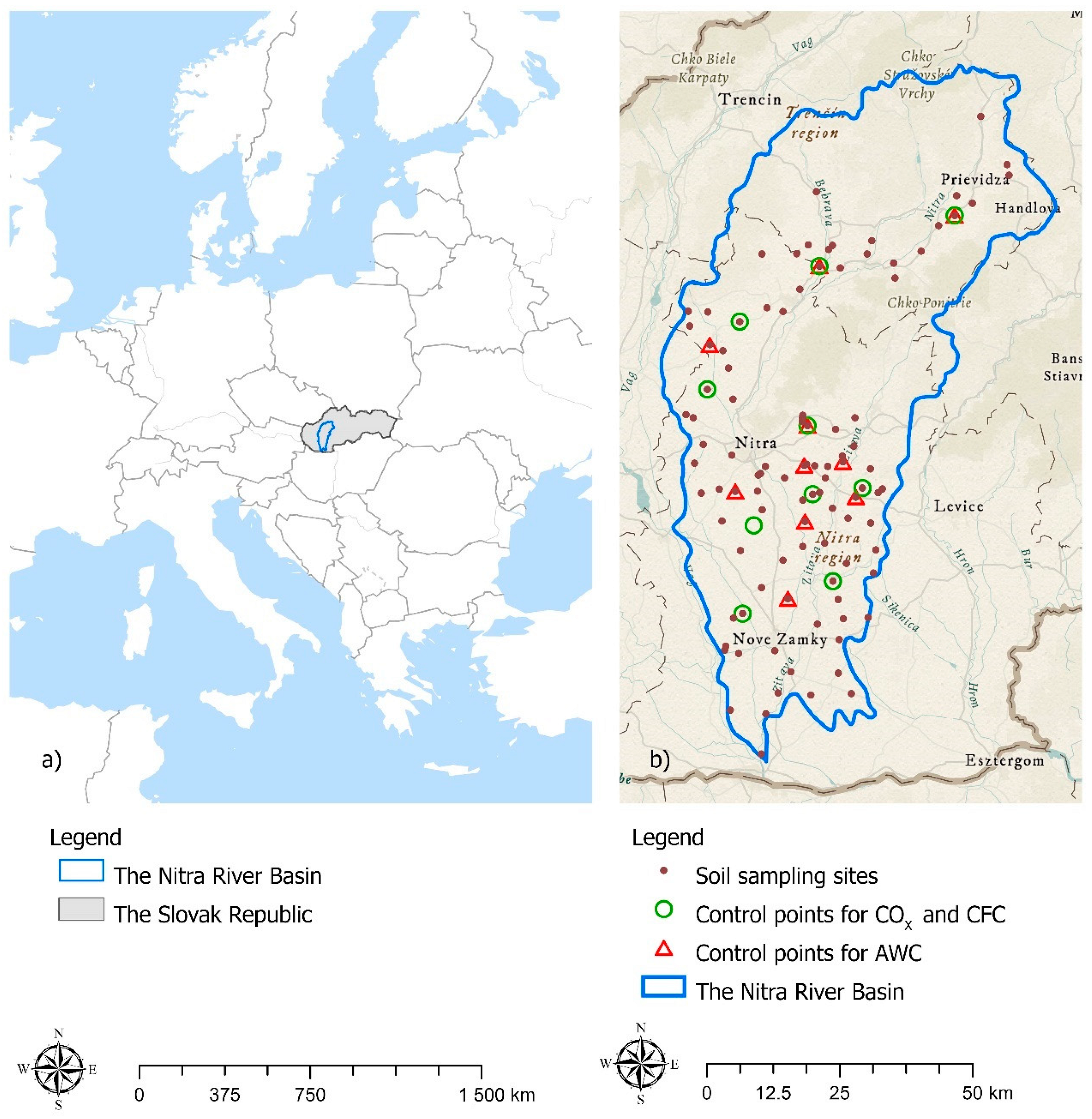
2.1. Study Site

The Nitra River Basin (Slovakia) with an area of 4501 km² is located in the western part of Slovakia (Figure 1a) to the west from Hron River Basin and to the south and west from the Váh River Basin. The Nitra River springs in the Malá Fatra mountains. It flows through the Prievidza and Hornonitrianská basins between the Tribeč, Žiar and Vtáčnik mountain ranges on the left side of the stream, the Strážovské vrchy, Malá Magura and Nitrické vrchy mountains to the right. The flow between the Tribeč and Považský Inovec mountains in the Podunajská pahorkatina forms a separate geo-morphological section of the Nitra River floodplain. The Nitra River then flows into the Váh River [38].

The altitude conditions of the Nitra River Basin vary within the range of 1238 m, with the highest point of the basin being the Vtáčnik Peak of 1346 m above sea level and the lowest being at the mouth of the river, 108 m above sea level. The average altitude of the basin is 326 m.

According to the orographic division, the territory is located in the orographic sub-system of the Carpathian Mountains and the Pannonian Basin [39]. The geologic structure of the upper layer of the Upper Nitra Basin and the Danube Uplands is formed by loess and loess clays, which represent the youngest geological period. The slopes and foothills of the mountains, the floodplain of the Nitra River and its tributaries are covered with deluvial sediments. These are mainly alluvial sediments with clayey-aluminous and gravelly facies [38].

Fluvisols, Cambisols, and Chernozems are the most represented soil types in the river basin, followed by Luvisols and Podzols. Agricultural land accounts for 69% of the river basin area. Forests cover 1430 km² of the basin, of which 892 km² are located in the upper part of the basin [17,40]. In terms of grain size distribution, light soils 3.7%, medium heavy soils, 77.9%, heavy soils 13.6% and very heavy soils 4.8% can be found in the Nitra River Basin [41].

In terms of climatic conditions, the basin belongs to three climatic areas. The warm climatic area occupies two-thirds of the territory and is located in the Danube Lowland, and in hollows and river sub-basins. The central part of the basin is located in the temperate climate area. The cold climate area has very little representation. Long-term average annual precipitation in the entire basin is 733 mm. In terms of climatic conditions, 65% of the basin belongs to a warm climatic area. The moderate climatic area is represented towards north of the basin, and the small area at the highest altitudes belongs to a cold climatic area. The mean annual temperature in the studied basin is within 7.5 to 10 °C [42].

2.2. Soil Sampling and Laboratory Soil Analyses

The location of sampling areas within the Nitra River Basin was determined according to maps of ESEU to obtain a network of sampling locations representing approximately the area of 6 × 6 km². The sampling point was chosen at least 300 m aside from the expected border of specific ESEU (there is a potential of its shifting within a year due to tillage etc.). Information on soil texture classes from maps of ESEU was used to ensure that the general percentage distribution of soil texture classes on the agricultural land in the basins would correspond to the representation of soil texture classes at the sampling sites. Soil sampling was conducted as a part of a bigger field survey, in which the disturbed and undisturbed soil samples were taken from the specific locations within the Nitra, Váh and Hron River Basins and were used for soil analysis of the basic physical and hydrophysical properties. This campaign and results were reported in the scientific monograph [39].

For the purposes of our study, we worked with 112 disturbed and undisturbed soil samples taken from agricultural land at a depth of 15–20 cm (Supplementary Materials Figures S1 and S2). The disturbed soil samples were taken using a spade and a shovel and were put in the numbered plastic bags. The undisturbed soil samples were taken using steel cylinders with a total volume of 100 cm³.

The disturbed soil samples were air-dried in the laboratory for at least 48 h, crushed and sieved on 2 mm mesh to remove gravel and roots. Soil organic carbon (CO_x) was determined by the wet combustion method of Tyurin [43], by oxidizing the organic matter using a mixture of 0.07 M H₂SO₄ and K₂Cr₂O₇ with titration using 0.01 M Mohr’s salt ((NH₄)₂SO₄ FeSO₄ 6H₂O). Prior to the soil texture analysis, carbonates (CaCO₃) were removed from another representative disturbed soil sample using 2 mol dm⁻³ HCl. The organic substances were removed by 6% hydrogen peroxide (H₂O₂). After repeated washing, the soil samples were dispersed with solution of 0.06 mol dm⁻³ sodium hexaphosphate (NaPO₃)₆ and 0.075 mol dm⁻³ sodium carbonate (Na₂CO₃). Clay fraction content <0.001 mm (CFC) was determined by the pipette method using pipette apparatus (Eijkelkamp Soil and Water, Giesbeek, The Netherlands) [44] (

Table 1. Overview of analyses performed for each soil sample.

Soil Parameter	Type of Analysis	Type of Soil Samples
		Disturbed	Undisturbed
Soil organic carbon (COx)	Wet combustion method of Tyurin [34]	x
Clay fraction <0.001	Pipette method [35]	x
Carbonates removal	Using 2 mol dm−3 HCl [35]	x
Organic substances removal	Using 6% hydrogen peroxide [35]	x
Field capacity (FC)	Pressure-plate method (−20 kPa) [36]		x
Wilting point (WP)	Pressure-plate method (−1500 kPa) [36]		x
Soil drying	Dried for 24 h at 105 °C [36]	x	x

).

The undisturbed soil samples were fully saturated and then placed to a pressure-plate apparatus (Soil Moisture Equipment Corp., Santa Barbara, CA, USA) to determine the volumetric water content corresponding to each pressure potential of field capacity (at a pressure potential of −20 kPa) and the wilting point (at a pressure potential of −1500 kPa). Prior to every increase of pressure potential, the undisturbed soil samples were weighed and the water content corresponding to each pressure potential was calculated. At the end, the soil samples were dried for 24 h at 105 °C in the oven and weighed [45]. The available water content (AWC) was calculated as the difference between the value of field capacity (FC) and wilting point (WP) (Table 1).

2.3. Software Used and Input Data Processing

Based on the individual laboratory measurements, the database containing positional point data of soil sampling sites (GPS coordinates and values of selected soil properties) was created focused on geodetic methods and measured data representing soil characteristics [46]. Finally, the spatial data were stored in a vector data format (shapefile, *.shp), which is suitable for working in the GIS software, as well as in the OpenGeo Suite environment [47]. ArcGIS (10.6, Esri, Redlands, California, USA) and GRASS GIS software (version 7.6, GRASS Development Team, https://grass.osgeo.org) were chosen for the purposes of this study. ArcGIS is a modular system and a commercial product requiring a license. GRASS GIS (Geographic Resources Analysis Support System) is GIS meant for spatial data management, image processing, graphics creation, spatial modeling and visualization of a large number of varied data types and unlike commercial GIS software GRASS is free. Its source code is available for review, modification, or updating. It is an official project of the NGO Open Source Geospatial Foundation. The GRASS GIS project is an international team effort that includes scientists and developers from various fields. GRASS has been under continuous development since 1982 involving a large number of federal US agencies, universities, and private companies. The development of core components and the management of releases were in charge of the Construction Engineering Research Laboratory (CERL) in Champaign, Illinois, USA. However, since 1997 a worldwide network of developers continues to develop and release of GRASS GIS. The GRASS GIS contains more than 500 modules for rendering maps and images, manipulating vector and raster data, including vector networks, creating, processing and storing spatial data [48].

2.4. Interpolation Methods Used in the Study

Interpolation methods [1,49,50] IDW, Spline, and Topo to Raster in ArcGIS and Regularized Spline with Tension method in GRASS GIS (GRASS GIS Spline) were used to create map layouts of the selected soil properties.

The inverse distance weighting (IDW) method determines cell values based on a linearly weighted combination of a set of entry points [51]. The output value for a cell is limited to the range of the values used to interpolate. Because IDW is a weighted distance average, the average cannot be greater than the highest or less than the lowest input. The optional parameter of weight “power” within the command controls the significance of surrounding points on the interpolated value. A higher power results in less influence from distant points. It can be any real number greater than 0. By increasing this value, the values of the nearest points will be emphasized, thanks to which they will have a higher impact on the resulting surface (which will also be less smooth). By decreasing this value, the points further from the currently calculated (interpolated) point will be of increasing importance and will affect the resulting value more. Since the IDW method is not tied to any physical process, it is generally not possible to determine which weight value (“power”) is most favorable. However, the most reasonable results can be obtained using values from 0.5 to 3 [52]. In our case this value was set to default 2, due to the irregular distribution of point source data. The search radius, limiting the number of known points for the interpolation of an unknown point in the output raster, was fixed to a minimum number of 12 points in our calculations.

Among the selected interpolation methods, the method of minimal curvature was the only one used in both ArcGIS (Spline) and GRASS GIS (Regularized Spline with Tension), in order to verify the credibility and reliability of its implementation in the relevant software. The spline method is characterized as a system of lower degree polynomials at different intervals, which follow up each other at the points of the input point field. Fajmon and Ružičková [53] presented several types of polynomial functions:

• Linear spline (first order)—Represents a set of linear functions that follow up each other in the specified (entry) points. It is actually a polyline connecting the points of the input point field. Its disadvantage is that the function has very sharp edges at specified points where it is not possible to determine the derivative. Not to mention that a linear spline can oscillate considerably from the actual surface between specified points.
• Quadratic spline (second order)—Characterized as a system of quadratic functions, which follow up each other at given points with a functional value as well as the value of the first derivative. Although a quadratic spline has better properties when compared to a linear spline, its downside is its inertia, as every two adjacent points are connected by a parabola that “shoots” a point until it takes the “right” direction to the next point.
• Cubic spline (third order)—Defined as a set of cubic functions that follow up each other at given points with a functional value, as well as with the first and second derivatives. The method shows very good properties as it passes through the given points and captures the course better than the parabola (there is a first and a second derivative at each point).

Most of the interpolation functions are based on previously known mathematical functions, which are based on a certain knowledge of the behavior of the observed geospatial phenomenon. However, we can look at the estimation of the values of geospatial phenomena in another way, by not knowing which mathematical function expresses them, but we know what values the function passes at certain points, and we try to estimate the course of the function using a point field of values. A multivariate spline belongs among the interpolation methods that try to find this function [54]. This method is also non-uniformly implemented in GRASS GIS and ArcGIS software.

The basic principle of a multivariate spline for modeling continuous phenomena (such as surfaces) from spatially distributed data is based on a physical model of a thin elastic membrane (plate), which we try to fit (as close as possible) through the points of the input point field by defining conditions for:

• flexibility of the function (tension parameter)
• smoothness of the resulting surface (smooth parameter).

The higher the tension value, the higher the flexibility and lower the stiffness. Higher values entered for the weight parameter result in somewhat coarser surfaces, but surfaces that closely conform to the control points. The values entered must be equal to or greater than zero. Typical values are 0, 1, 5, and 10. The Weight is the square of the parameter referred to in the literature as phi (Φ) [55]. In the case of lower tension, the lower flexibility and higher stiffness is manifested by a smooth surface but without the possibility of the function passing through the entry points.

Each part of the surface is expressed by a separate polynomial function (most often cubic), which is derived from the local values of the input point field. The course of the function is affected by several conditions. The basic condition is that the continuity of adjacent polynomial functions at the points of the input point field is ensured.

The ArcGIS interface offers two types of spline interpolation—regularized and tension separately without the possibility of their “simultaneous” use. The “Regularized” option modifies the minimization criterion derived from 3rd order polynomial functions and weighting parameters. The result is a smoother surface, including its first derivative. The “Tension” option modifies the minimization criterion by derivation from first-order polynomial functions and weighting parameters. The result is a smoothed surface—its first derivative is continuous; however, it is not smoothed [56]. Both options (which create significantly different surfaces) interpolate the surface in spatial blocks (regions) depending on the input settings. In this work, the “Regularized” option was selected which was controlled by the weight parameter of 0.1 defining the smoothness of the resulting surface.

On the other hand, the GRASS GIS environment integrates the regularized spline with the tension [57], which determines the nature of the resulting surface, and thus provides more favorable results (qualitative and visual) not only in topography but also in groundwater modeling (groundwater flow modules), soil conditions, etc. This method was proposed by the authors Mitašová, Hofierka and Zlocha [58] as “completely regularized spline with controllable oriented tension and regular derivatives of all orders”. The aim of the authors was to remove or mitigate the shortcomings of a thin plate spline method, the application of which (e.g., in the ArcGIS environment) raises problems both in interpolation in areas with a rapidly changing gradient (formation of false extremes) and in the calculation of second-order derivatives (logarithmic singularities). The newly developed method was subsequently implemented in the GRASS GIS environment as the v.surf.rast module. It is a precise method; however, it requires a deeper knowledge of the influence of its parameters (not only basic) on the result. On the other hand, its use is simpler than in the case of kriging methods [59]. The tool allows sensitive setting of the spline function thanks to the simultaneous use of the parameters of tension (regulating the flexibility of the function) and smoothing (regulating the exactness of the function). The module also allows using cross-validation for setting the appropriate parameter values. It works in batches with 700 entry points at once. In the case of a larger number of input point fields, the segmentation occurs. GRASS GIS does not work directly with *.shp data formats, but thanks to its tools, importing and subsequent use of data is possible. Further information on GRASS GIS Spline method can be found in the works of Mitasova, Mitas and Harmon [60] and Neteler and Mitasova [61].

The Topo to Raster method is based on the ANUDEM program [62,63], which was developed by ESRI to generate hydrologically correct digital relief models (DMR). The interpolation procedure has been designed to take advantage of the types of input data commonly available and the known characteristics of elevation surfaces. This method uses an iterative finite difference interpolation technique. The method is optimized for the computational efficiency of local interpolation methods (such as IDW), but without losing the surface continuity of global interpolation methods (such as Spline). It is essentially a discretized thin plate spline technique for which the roughness penalty has been modified to allow the fitted DEM to follow abrupt changes in terrain [64]. Because of its favorable properties, this method was also included among the selected interpolation methods in this study. Due to the non-elevation input data (i.e., soil properties), we prevented the possible removal of “surface depressions” (no enforce) as part of the emphasis on drainage enforcement.

2.5. Data Processing and Verification of the Results

The calculations were preceded by the processing of input vector data (point data, i.e., sites of soil sampling, measured using GPS and areal data, i.e., the boundaries of the Slovak river basins provided by Slovak Hydrometeorological Institute in Bratislava, Slovakia), consisting of their transformation into a singular coordinate system (S-JTSK Krovak East North, EPSG code 5514) and converting them into a shapefile (*.shp) interchange format. In order to avoid extrapolations, in addition to soil samples of the Nitra River Basin, spatial information on the soil samples of neighboring river basins (Váh, Hron and Danube River) was also used. The subject of interpolation consisted of point vector data (in shapefile format), as well as information on soil properties such as AWC, CO_x and CFC. Both sets of input spatial data were originally in the coordinate system WGS 1984 or, more precisely, after transformation also in the SJTSK Krovak East North coordinate system. The same spatial parameters were used to analyze the most suitable interpolation method (via their mutual comparison). We set the raster output cell size (i.e., resolution) to 50 m in each interpolation method, and the Nitra River Basin boundary was chosen as the interpolation range (or mask).

To verify the accuracy of the results, the interpolated values of the selected soil properties were cross-checked with the measured values. From the database, 10 sites were randomly selected as control points for verification and excluded from further spatial processing. After the fully random selection, the control points were crosschecked against some specific criteria—namely, representativeness of the geomorphological units and the soil types occurring within the agricultural land in the basin. At the same time, the sites were located outside the significant horizontal curvature of the relief (i.e., outside the ridge, valley). While the same control points were used for CO_x and clay fraction content, a different set of 10 control points was chosen for AWC (Figure 1b). Subsequently, all four interpolation methods were repeated, but with the exclusion of measurements from 10 control points. Using the zonal statistics function, we found the values of available water capacity, CO_x content and particle size fraction of <0.001 mm content in interpolated raster maps calculated without control points. Subsequent comparison of the detected (interpolated) values with measured (original) values defined the accuracy of the given interpolation method. The second criterion for evaluating interpolation methods was the reliability according to visual inspection of interpolated raster maps produced from the overall database.

3. Results

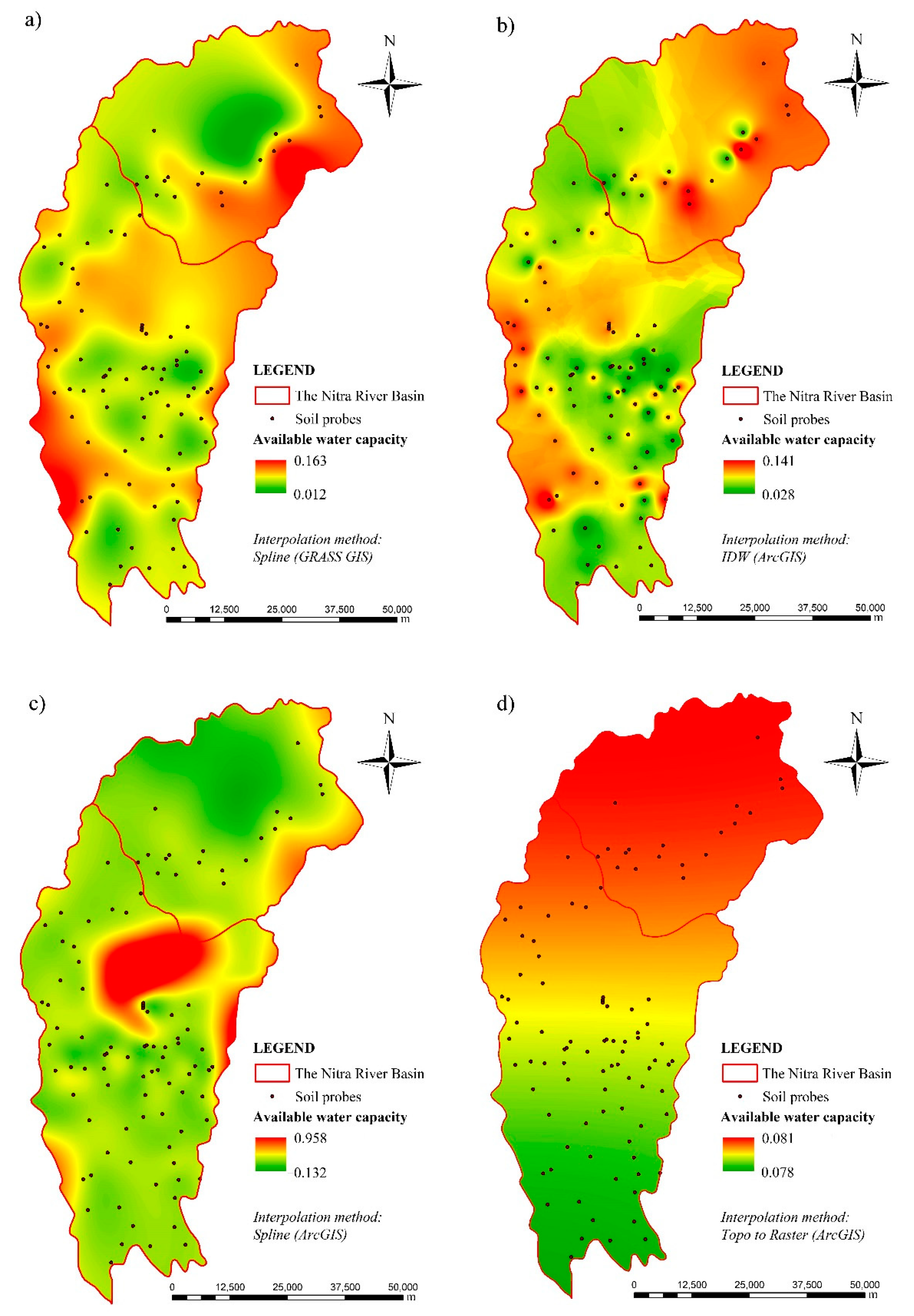
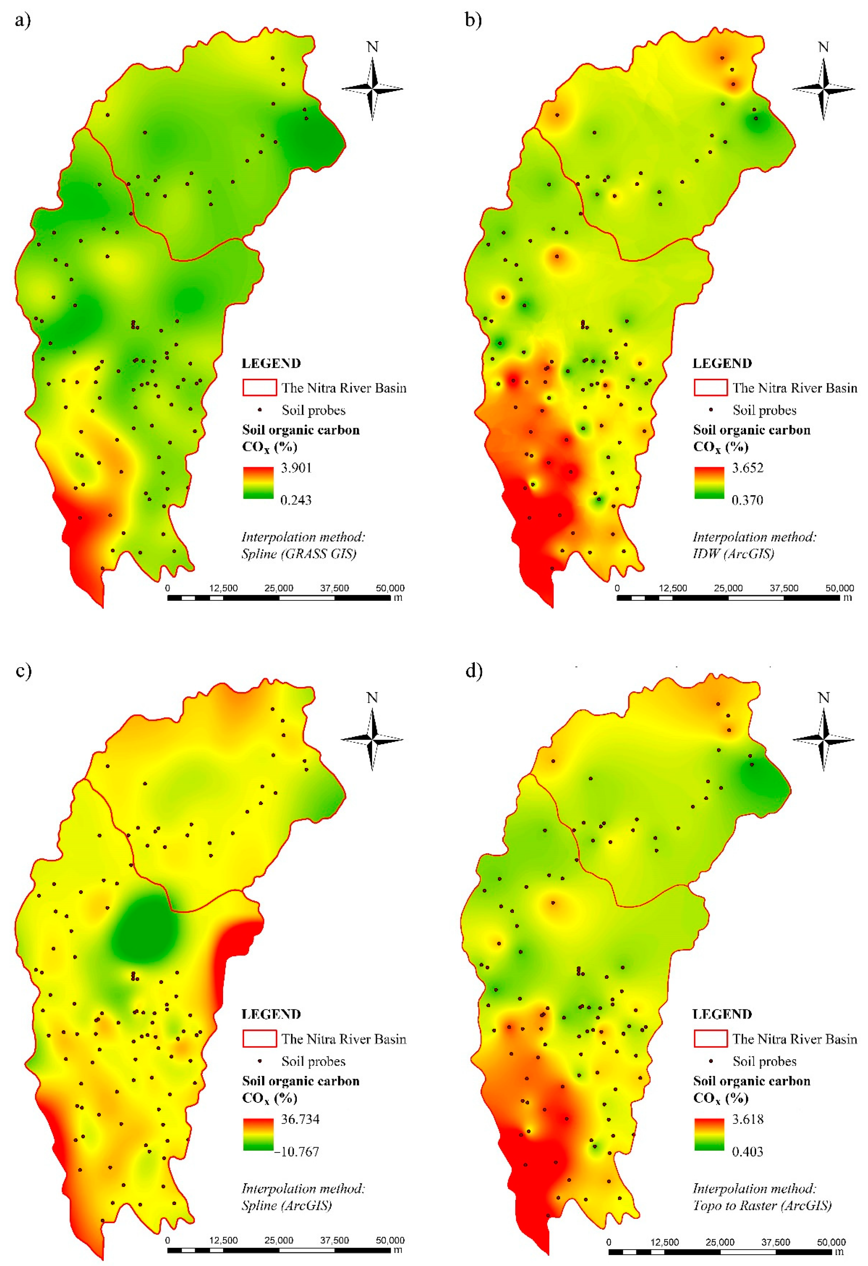
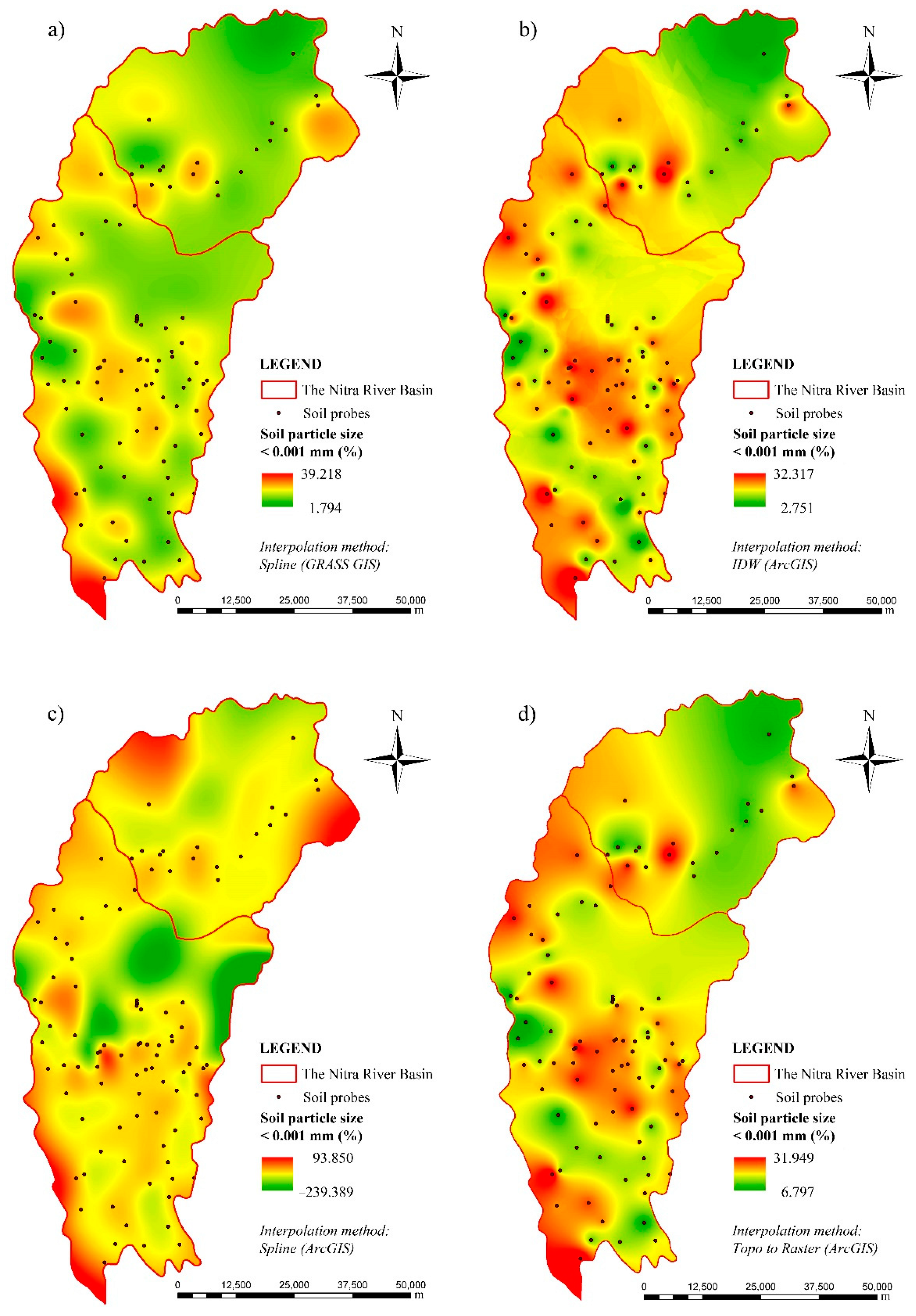
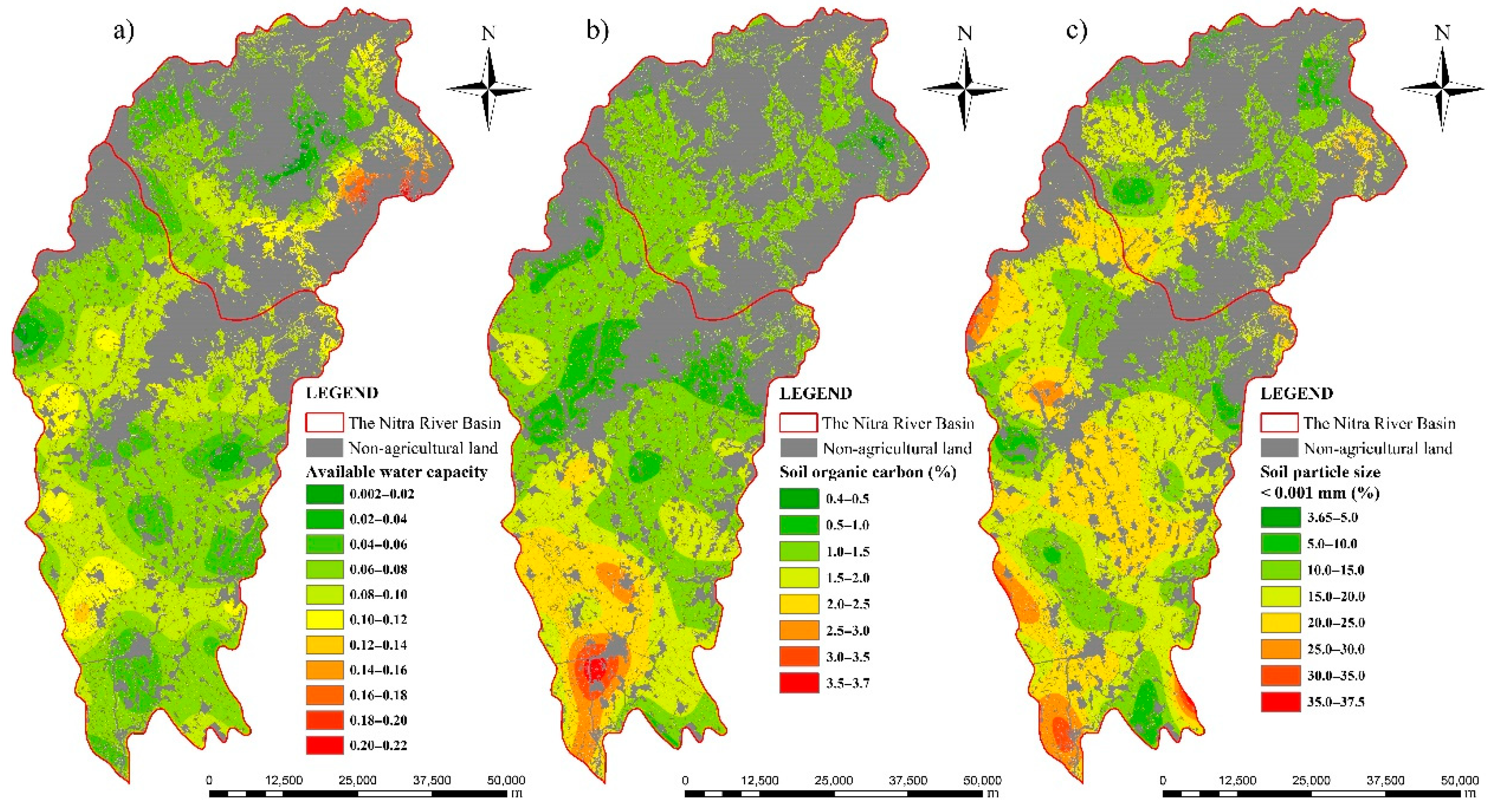
3.1. The Maps of the Interpolated Soil Properties

The spatial distributions of interpolated values from 112 sampling points for available water capacity (AWC), soil organic carbon content (CO_x) and content of clay fraction <0.001 mm (CFC) in raster format are presented in Figure 2, Figure 3 and Figure 4. Considering the conditions of the soil sampling, it is necessary to emphasize that the interpretation of the values is valid only in the extent of agricultural soils and the soil layer in the range 15–20 cm. AWC, which represents the amount of water in the soil between the field capacity and wilting point was expressed in cm³ cm⁻³. The input AWC from 112 sampling points ranged from 0.028 up to 0.141 cm³ cm⁻³. The interpolation method Topo to Raster resulted in a dataset with a very narrow range of values (0.078–0.081 cm³ cm⁻³) (Figure 2). On the contrary, after using Spline (ArcGIS) the interpolated values were in a very wide range from −0.132 cm³ cm⁻³ up to 0.958 cm³ cm⁻³. With this interpolation method even non-realistic negative values of AWC were obtained. The range of the dataset obtained by Spline in GRASS GIS was very similar to the input (from 0.012 cm³ cm⁻³ up to 0.163 cm³ cm⁻³), while the range of the values after interpolation using IDW was identical with the source data (from 0.028–0.141 cm³ cm⁻³).

Content of organic carbon (CO_x) was expressed in %. The input CO_x from 112 sampling points ranged from 0.37 up to 3.65%. Once again, the interpolation method Topo to Raster resulted in dataset with the narrowest range of the values (0.37–3.65%) (Figure 3). Interestingly, it was similar as the set of input data; however, similar minimum and maximum values were observed also for the Topo to Raster method. The range of the dataset obtained by Spline in GRASS GIS was wider (0.24–3.90); however, the values were all above zero. After using Spline (ArcGIS), the interpolated values were again in a very wide range from −10.77% up to 36.73%, including also negative values of CO_x.

Representation of the clay fraction (CFC) (content of particles with diameter <0.001 mm) was also expressed in %. The input CFC from 112 sampling points ranged from 6.8–32.4%. Once again, the interpolation method Topo to Raster resulted in dataset with the narrowest range of the values (6.8–31.9%) (Figure 4). However, a similar maximum value was observed also for the IDW method. The minimum value was closer to dataset obtained after interpolation using Spline in GRASS GIS (values in the range 1.8–39.2%). The range of the dataset obtained by Spline in GRASS GIS was wider than for IDW and Topo to Raster methods (in the range 1.8–39.2%) but again, the values were all above zero. After using Spline (ArcGIS), the interpolated values were again in a very wide range from −239.4% up to 93.9%, including also incorrect negative values of CFC.

3.2. Evaluation of the Accuracy and Reliability of Interpolation Methods

The suitability of the used interpolation methods for spatial modelling of distribution of heterogenic soil properties was based on two evaluation criteria: accuracy and reliability. The accuracy of interpolation was evaluated by comparison of the measured values at control sites with the interpolated values for the same locations. The observations of these comparisons for AWC, CO_x and CFC are shown in

Table 2. Evaluation of the accuracy of available water capacity interpolation.

Control Points	Measured Value (cm3 cm−3)	Interpolated Value (cm3 cm−3)
		Topo to Raster	IDW	ArcGIS Spline	GRASS GIS Spline
1	0.140708	0.080216	0.075749	0.075214	0.072174
2	0.061371	0.081247	0.073719	0.051791	0.064542
3	0.093481	0.078578	0.083541	0.090395	0.091835
4	0.088599	0.081825	0.072589	−0.071627	0.052250
5	0.049038	0.082730	0.089260	0.094883	0.089997
6	0.080558	0.081047	0.097605	0.159259	0.095610
7	0.028343	0.079983	0.051309	0.040055	0.045009
8	0.036007	0.080684	0.073597	0.072663	0.076360
9	0.094971	0.079156	0.090561	0.090148	0.061163
10	0.058641	0.079792	0.076479	0.076191	0.072844
Absolute difference between measured and estimated value (cm3 cm−3)		Category of interpolation accuracy
0.001–0.02		Very accurate
0.02–0.03		Accurate
0.03–0.04		Medium Accurate
0.04–0.05		Less Accurate
0.05–0.06		Inaccurate
0.06–0.065		Very inaccurate

,

Table 3. Evaluation of the accuracy of soil organic carbon content interpolation.

Control Points	Measured Value (%)	Interpolated Value (%)
		Topo to Raster	IDW	ArcGIS Spline	GRASS GIS Spline
1	1.131	1.086831	1.354055	1.767087	1.324685
2	1.324	1.311159	1.178453	1.251359	1.257256
3	0.976	1.444001	1.275493	1.661232	1.403020
4	1.231	1.176385	1.181107	1.317056	1.241724
5	2.136	1.603976	1.762339	1.136238	1.599983
6	1.038	2.935651	2.827492	2.658278	2.904012
7	1.223	1.306799	1.484810	1.526687	1.412650
8	1.782	1.103724	1.072056	1.860530	1.112799
9	1.048	1.049305	1.347805	−0.625535	1.372697
10	1.102	0.723665	1.302310	0.816751	1.337883
Absolute difference between measured and estimated value (%)		Category of interpolation accuracy
0–0.25		Very accurate
0.25–0.5		Accurate
0.5–0.75		Medium Accurate
0.75–1		Less Accurate
1.0–1.7		Inaccurate
1.7–2		Very inaccurate

and

Table 4. Evaluation of the clay fraction content <0.001 mm interpolation.

Control Points	Measured Value (%)	Interpolated Value (%)
		Topo to Raster	IDW	ArcGIS Spline	GRASS GIS Spline
1	12.95	15.942033	16.444836	16.947046	14.745194
2	10.97	12.822754	13.441525	13.222441	12.676295
3	25.63	15.349472	15.221250	21.669676	14.300347
4	15.22	16.811474	17.843370	20.834646	17.150152
5	13.54	20.639168	20.057674	20.640047	20.076025
6	12.86	27.390329	25.834656	27.440178	27.262318
7	18.15	13.589706	15.183517	16.064138	13.071733
8	15.97	18.780331	17.528008	25.027676	19.278391
9	20.02	15.640176	16.217323	21.878086	14.461142
10	20.59	21.456535	20.932981	23.383768	21.760553
Absolute difference between measured and estimated value (%)		Category of interpolation accuracy
0–2.5		Very accurate
2.5–5.0		Accurate
5.0–7.5		Medium Accurate
7.5–10		Less Accurate
10–12.5		Inaccurate
12.5–15.0		Very inaccurate

. In the case of evaluation of the accuracy of AWC values (Table 2), IDW was the most accurate interpolation method on the basis of cross-classification, as 60% of the compared values (measured vs. estimated) were within the absolute difference margin up to 0.02 cm³ cm⁻³. The same trend was observed for the GRASS GIS Spline method; however, there was 10% more points with less accurate interpolation (difference in the range of 0.04–0.05 cm³ cm⁻³). In the case of the Topo to Raster method, the interpolation accuracy was more variable, and the ArcGIS Spline method proved to be the least accurate since the values of 30% of interpolated points were very inaccurate.

Regarding CO_x values cross classification (Table 3), 50% of the interpolated values were very accurate and 20% accurate in the case of Topo to Raster and GRASS GIS Spline methods. The IDW interpolation method resulted in 40% of very accurately estimated values and 40% of accurately estimated values. However, these two favorable categories were observed only in case of 50% of compared values in the case of the ArcGIS Spline method.

The GRASS GIS Spline method was shown to be the most accurate also when comparing the measured and estimated values of CFC from 10 sampling sites as 40% of estimated values were very accurate (10% more than in case of other methods) (Table 4). The accuracy of Topo to Raster and IDW methods was the same as 70% of the estimated points and were accurate or very accurate. At the same time, the level of accuracy was the same for the majority of the compared points. The ArcGIS Spline interpolation method was the least accurate.

Based on the knowledge of the spatial distribution of hydrophysical properties of soils, the visual check of the outputs was conducted. We concluded that the GRASS GIS Spline method was the most reliable method for AWC values estimation. At the same time, the mean difference resulting from cross-validation of the measured and estimated values was the lowest (0.00099 cm³ cm⁻³). The GRASS GIS Spline method was also the most reliable in case of CO_x and CFC, where the mean difference was 0.19% and 0.88%, respectively.

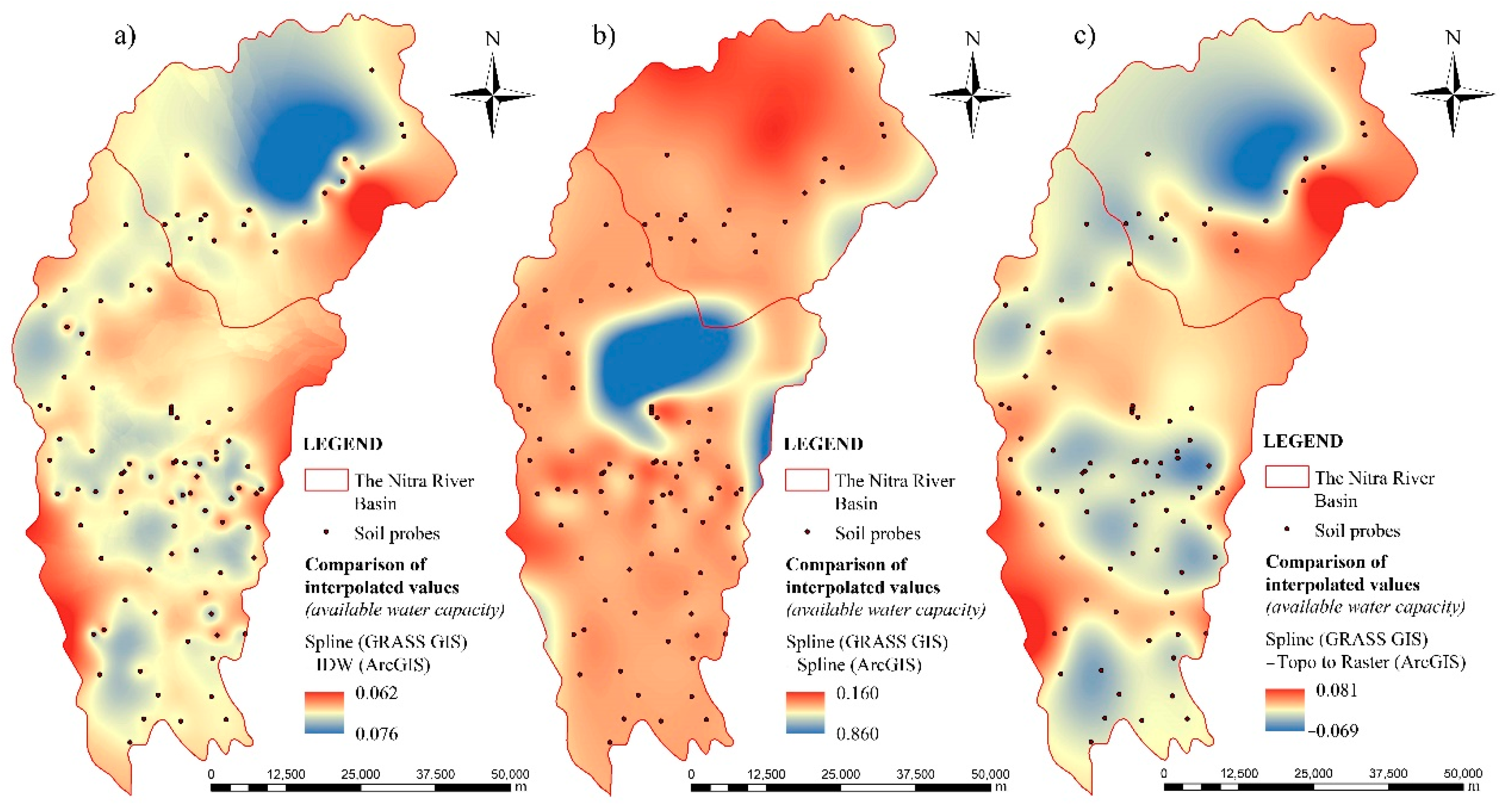
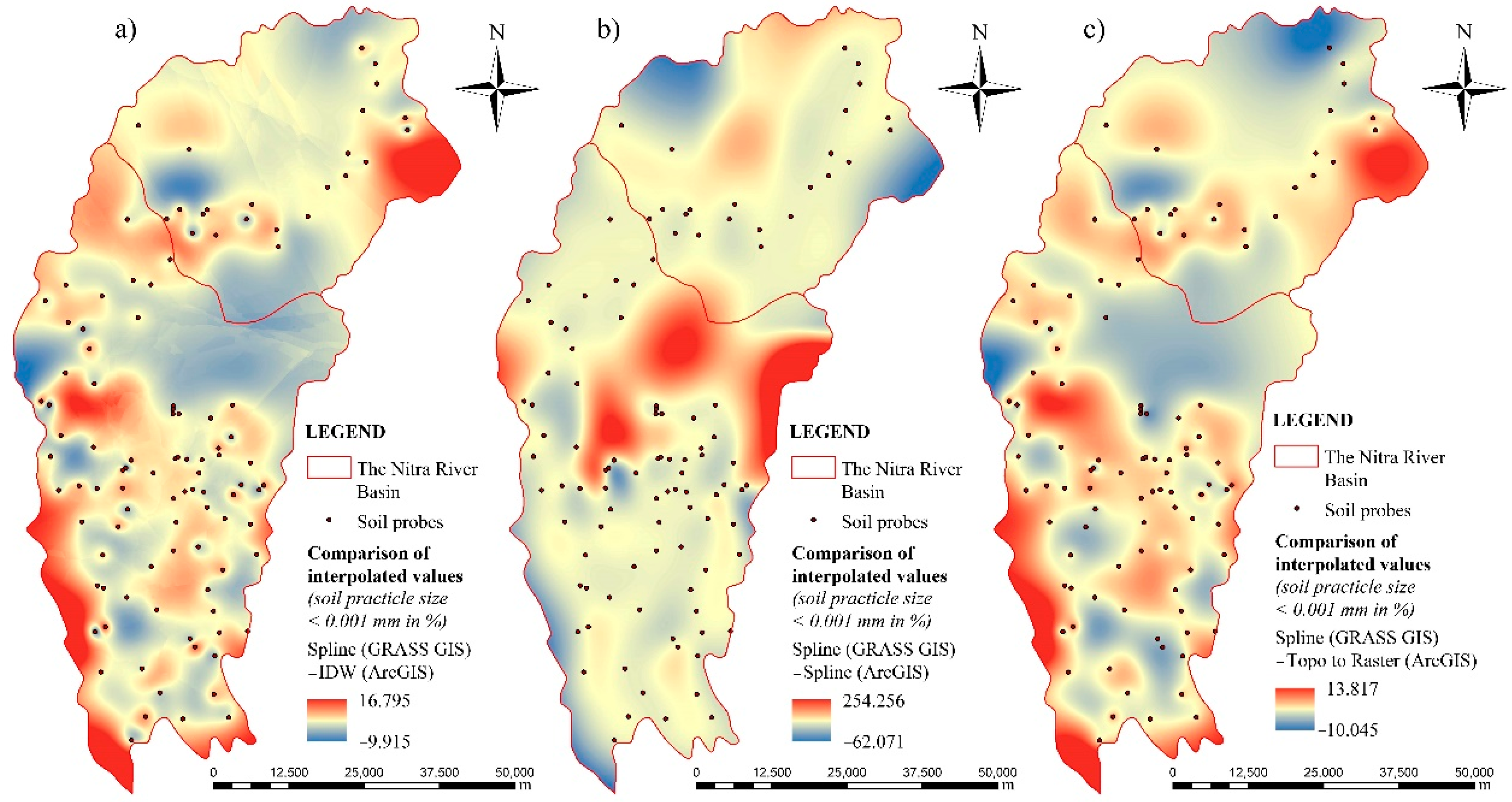
3.3. Comparison of GRASS GIS Spline Method with Other Interpolation Methods and Final Processing

In the following step, the values obtained by the GRASS GIS Spline interpolation method (as the most accurate and most reliable method with respect to the selected criteria described above) were compared with the outputs of the interpolation methods IDW, Topo to Raster and ArcGIS Spline. The comparison was processed in GIS using the Raster Calculator function as a calculation of the difference between the interpolated values GRASS GIS Spline and other interpolation methods used in this study. From the resulting raster maps (Figure 5, Figure 6 and Figure 7), we spatially determined the interpolation deviations (IDW, Topo to Raster, or ArcGIS Spline) as compared to the GRASS GIS Spline method.

The comparison shows that Topo to Raster tends to interpolate values based on an algorithm that is primarily adapted to work with contour data, and the main factor influencing shape modeling are the hydrological processes [65].

We can state that the interpolations with Topo to Raster are generally favorable, although with slightly elevated values in the vicinity of the points compared to the GRASS GIS Spline. With the IDW interpolation method, we can observe strong influence of values in the individual points on their surroundings. On the other hand, the ArcGIS Spline method showed extreme values in the absence of input source data (or in the case of irregular or insufficient coverage). The greater the distance of the soil probes when studying the individual hydro-physical characteristics, the more clearly the adverse consequences of the interpolation method became apparent.

From the differences obtained by comparing interpolation methods, we calculated the mean and standard deviation by statistical processing in GIS, which are shown in

Table 5. Comparison of interpolation methods by the differences in their values at the raster cell level.

Soil Properties	Spline (GRASS GIS)–Topo to Raster	Spline (GRASS GIS)–Spline (ArcGIS)	Spline (GRASS GIS)–IDW
	Mean ± Standard Deviation	Mean ± Standard Deviation	Mean ± Standard Deviation
Available water capacity (cm3 cm−3)	−0.00004 ± 0.024	−0.039 ± 0.142	−0.00068 ± 0.0195
Soil organic carbon (%)	0.063 ± 0.191	0.027 ± 2.654	0.0095 ± 0.227
Clay fraction content <0.001 mm (%)	0.667 ± 2.462	4.051 ± 22.143	−0.167 ± 3.321

.

As the survey of soil properties was carried out only on agricultural land, the maps produced by Spline interpolation (GRASS GIS) were subsequently modified only for the visualization of agricultural land. This reduction took place using the Land Parcel Identification System (LPIS) database, showing the vector layer of production blocks at the level of the entirety of Slovakia. The maps in Figure 8 present the final distribution of individual analyzed soil characteristics within the Nitra River Basin. Grey areas in the map layouts represent the forests. The displayed interpolated values using the GRASS GIS Spline method best corresponded to the measured reality in the field. Certain inaccuracies between the measured and modeled values could arise from insufficient coverage of the area by input data (sampling sites)—due to the nature (configuration) of the terrain, inaccuracies in sampling and analyzes performed in the laboratory. The values of the increased CO_x content shown on the map coincide with the localities where there are areas of fertile organic matter-rich, predominantly loamy soils. These are areas of the alluvial, flatter part of the basin. In the upper part of the basin there are soils with a shallower soil horizon with predominantly loam-sandy and sandy soil with a lower CO_x content.

4. Discussion

4.1. Comparison of the Interpolation Methods Used in the Study

The Spline (ArcGIS) interpolation method provided also negative values for interpolations of selected soil properties (AWC, SOC, CFC). This method was implemented using ArcToolbox Spatial Analyst—an interpolation tool where user rights are limited to the choice of the type of method used (Regularized, Tension) and parameters (Weight, Number of points) [66], and the user cannot modify the used algorithm. Therefore, the implemented interpolation does not guarantee that the values will not fall outside the range of input data in the intervention space. However, various approaches are known, e.g., using local algorithms for the construction of non-negative cubic splines [67], which are based on a natural spline, in which the negative values are redefined by adding extra knots to this interval. By using the optimization criterion, an optimal spline is subsequently obtained in which the strain energy is minimized. The mathematical properties of the new rational cubic spline are the subject of a detailed examination in the work of Karim [68]. This is a new method used to maintain positivity and limited interpolation of data over any line. Modification of the interpolation curve shape is ensured by derived parameters. The authors Bogdanov and Volkov [69] also dealt with shape-safe cubic splines and they developed methods ensuring a positive cubic spline (including its derivatives) for a positive function (or a function with a positive derivative). In case of ArcGIS, more options for setting spline parameters are provided by the Geostatistical Analyst extension (ArcToolbox—Geostatistical Analyst—Interpolation). However, it also requires more knowledge for choosing the suitable methods and setting their parameters [70]. Therefore, the GRASS GIS module—Regularized Spline with Tension—was also used in our study.

The reason why such a “similar”, at least based on the name, Spline interpolation method produced such divergent results in two GIS applications (GRASS GIS and ArcGIS) would be due to the fact that the RST algorithm in GRASS GIS uses tension and smoothing. Both presented parameters change the character of the approximation mathematical function. While the smoothing parameter controls the height deviation at the nodes of the RST approximation, the tension parameter speaks to the stiffness of the approximation function. A high value of tension gives the function the character of an elastic membrane or, in case we use a comparison with rubber, the character of an elastic and soft rubber band. The spline of a thin plate (ArcGIS Spline) modeling surface with higher values of tension is getting closer and closer to their real heights at the nodal points of the RST approximation, but large height deviations can occur in their immediate vicinity. In places of significant changes of (given) values of the real area, due to the greater flexibility of the function, there is often a “bulge” of the created model, e.g., the formation of false depressions or peaks (singularities), as we can observe in the case of the content of the clay fraction with a value up to a by far unrealistic −240% (Figure 4). Conversely, a low tension value gives the approximation function the character of a thin plate (i.e., the character of a hard and unyielding rubber). The decrease in tension values in the nodal points of the RST approximation manifests itself by ever greater deviations of the projected heights from the heights of the points of the input height field, but in their vicinity, there are no such significant height deviations to be found. Therefore, due to the implementation of the thin plate spline in the ArcGIS environment, specific problems arose both with the interpolation in areas with a rapidly changing gradient (formation of false extremes) and in the calculation of second order derivatives (logarithmic singularities). Moreover, the absence of the tension parameter was subsequently manifested by the undesirable representation of false extremes. Tension option was not used because of application of the linear spline. On the contrary, the RST algorithm in the GRASS GIS environment was highly sufficient in the case of the Nitra River Basin sampling sites as is set up to be able to work with 700 entry points at a time without restrictions (otherwise the point field would be segmented).

Differences to some extent in our observations regarding the values of accuracy (as a difference between the measured value and the estimated value according to interpolation methods used in the study) could occur in case of using a different set of control points for interpolation accuracy verification. However, we do not assume that there would be significant difference in the results, regarding the evaluation of the suitability of the used interpolation methods as the reliability of the methods was assessed also visually. Based on the observed results in our study, the GRASS GIS Spline method was shown to be the most suitable method for estimating the spatial distribution of soil properties such as AWC, CO_x and CFC.

4.2. Applicability of Interpolation Methods Used in the Study in Soil Science

To compare interpolation methods regarding the spatial distribution of soil organic carbon soil (SOC), Bhunia, Shit and Maiti [35] used 98 randomly taken samples (for different kinds of land use—agricultural land, forests, TTP, NDV) in three different soil depths (0–20 cm, 20–40 cm and 40–100 cm). The accuracy of selected interpolation methods (inverse distance weighting (IDW), local polynomial interpolation (LPI), radial basis function (RBF), ordinary kriging (OK) and Empirical Bayes kriging (EBK)) was evaluated by cross-validation using a coefficient of determination (R2) and RMSE. The ordinary kriging (OK) method has shown itself to be the best for use in interpolating the spatial distribution of the SOC.

Srivastava et al. [36] have also analyzed the properties of agricultural soil (soil moisture) using various interpolation methods (IDW, ordinary kriging (OK), kriging with external drift (KED) and Spline). In their work, they used the ArcGIS v10.1 software (Esri, Redlands, California, USA). They used point values from 82 sites (Varanasi, India), following the 2:1 rule, and thus used two thirds (54 sites) for calibration and one third (28 sites) for validation of outputs. They concluded that the KED and OK methods, then IDW and finally Spline were the most suitable for modeling of hydro-physical soil properties, such as water content, which confirms our conclusions when we also evaluated the Spline (ArcGIS) method as the least suitable and IDW as relatively accurate.

Although the OK method showed big potential in the above-mentioned studies, it was not used in our study as its application is more complex than GRASS GIS Spline. With this method, the weights depend not only on the distance between the measured points and the predicted location, but also on the spatial arrangement of the measured points around the location of the predicted value. To be able to use the spatial arrangement of measured points (sampling points of the Nitra River Basin) for the calculation of weights, the spatial autocorrelation (or dependence) must be determined. The spatial autocorrelation of a phenomenon with respect to distance and direction of action is expressed by a semivariogram with its geostatistical parameters such as nugget variance, structured variance, sill variance or distance parameter. Looking at the spatial data distribution within the study area (Figure 1), we can observe that while in the southern part of the Nitra River Basin there is a random but mostly uniform distribution of data, further north this distribution changes to a random uneven point, up to profile distribution (data concentration in the Nitra River valley). Considering these facts, the correct determination of spatial autocorrelation is considerably more difficult. On the other hand, recognizing the considerable potential of OK, it might be a suitable interpolation method for our purpose, but only after an additional increase of sampling point network density in the northern part of the basin, as agricultural land is not located exclusively in the river valley, but it extends up to the forest stands (Figure 8). Otherwise, the potential of the OK method would not be adequately exploited.

Ghosh and Pekkat [37] used interpolations in spatial analysis of another one of the hydro-physical soil properties, namely the hydraulic conductivity. In their work, they evaluated the methods of Kriging, IDW, Natural Neighbor, Spline and Trend. The ArcGIS software, version 10.3.1, was also used in this study. The study was conducted in Brahmaputra, India. They performed interpolation on the basis of point values in two areas out of 14, or 6 sites respectively. The data from three independent points were used to compare accuracy. The results of this study showed that the best results (the smallest RMSE) were obtained via different variants of the kriging method. The IDW, Natural Neighbor, Spline and Trend methods followed in terms of accuracy. Thus, this study also partially confirms our results when IDW was evaluated as more accurate than Spline (ArcGIS).

Obtaining spatial data on soil by interpolation is undoubtedly a method with many benefits. This method of obtaining spatial information is also described in work of Vereecken et al. [71] In a GIS environment, they recommend using methods of variogram analysis or kriging, although this was not included in our study. Several authors mention and use the kriging method in their work, for example [72,73,74]. Pecho [75] evaluated the kriging method as being able to more accurately interpolate and estimate the investigated values even in areas with lower point network density using direct measurements.

When choosing the right interpolation method, the amount, distribution and nature of the input data must also be considered. Čimo et al. [76] therefore preferred the Topo to Raster method in ArcGIS, for its combination of the IDW, Spline and Kriging methods. Methods of spatial interpolation of different soil properties are, among other things, directly proportional to the representation and spatial distribution of input data. The suitability of using selected interpolation methods with a limited amount of input data (i.e., at a coarser scale) of selected soil properties (sand, slit, clay, pH, base saturation, organic matter, etc.) was investigated by Schloeder, Zimmerman and Jacobs [77], while including methods such as ordinary kriging, inverse-distance weighting, and thin-plate smoothing splines with tensions. The results indicated that spatial interpolation was adequate when the data showed smooth and consistent patterns of spatial dependence within the studied area and the selected range of estimates and weights used in this study. Ordinary kriging and inverse-distance weighting were similarly accurate and effective methods; thin-plate smoothing splines with tensions were, however, not. Thus, the authors pointed out that the sample size is as important for research on a coarse scale as it is on a fine (accurate) scale with a rich representation of soil data. Such geostatic operations achieve sufficient results and are useful for the spatial determination of soil and other properties [78].

5. Conclusions

There is an increasingly growing demand for spatial information among professionals, including the characteristics of agriculturally used land. In the case of soil properties, we rely on a specific amount of point data, which in turn creates the need to convert them into surface expressions. To meet this need, we paid attention to GIS applications in relation to soils in this study. Comparison of the most often used interpolation methods such as Spline, IDW and Topo to Raster in ArcGIS and Spline in GRASS GIS was based on measured and interpolated values of available water content, soil organic carbon content and clay fraction content. According to our observations, Spline (GRASS GIS) and IDW (ArcGIS) interpolation methods were shown to be the most accurate and reliable. The most precise estimates were observed for values of AWC, when according to verification with field measured data, both interpolation methods (GRASS GIS Spline and IDW) resulted in 60% of values with a high accuracy. In the case of CO_x, 50% and 40% of the values were estimated very accurately using GRASS GIS Spline and IDW methods, respectively. The accuracy of the estimates was lower in the case of clay fraction content <0.001 mm, 40% and 30% in case of GRASS GIS Spline and IDW, respectively. We assume, that these methods are suitable for interpolation of selected soil properties in conditions similar to our study basin in Slovakia. On the contrary, the Spline method in the ArcGIS environment (with the implementation of a thin plate) proved to be unusable due to the occurrence of false extremes. The results could be affected also by the influence of the relief fragmentation on the accuracy of interpolation, showing the potential need for increasing the concentration of source data depending on the morphological properties of the river basin. The validity of our conclusions from interpolations in the case of other soil properties can only be confirmed or refused through further research in this area.

References

1. Hlásny, T. Geographic Information Systems—Spatial Analysis; Zephyrosy: Zvolen, Slovakia, 2007. [Google Scholar]
2. Tárník, A.; Igaz, D. Quantification of soil water storage available to plants in the Nitra River Basin. Acta Sci. Pol. 2015, 14, 209–216. [Google Scholar] [CrossRef]
3. Bárek, V.; Halaj, P.; Igaz, D. The Influence of Climate Change on Water Demands for Irrigation of Special Plants and Vegetables in Slovakia. In Bioclimatology Natural Hazards; Springer: Dordrecht, The Netherlands, 2009; pp. 271–282. [Google Scholar]
4. Boubehziz, S.; Khanchoul, K.; Benslama, M.; Benslama, A.; Marchetti, A.; Francaviglia, R.; Piccini, C. Predictive mapping of soil organic carbon in Northeast Algeria. Catena 2020, 190, 104539. [Google Scholar] [CrossRef]
5. Muchová, Z.; Leitmanová, M.; Petrovič, F. Possibilities of optimal land use as a consequence of lessons learned from land consolidation projects (Slovakia). Ecol. Eng. 2016, 90, 294–306. [Google Scholar] [CrossRef]
6. Mikloš, M.; Igaz, D.; Šinka, K.; Škvareninová, J.; Jančo, M.; Vyskot, I.; Škvarenina, J. Ski piste snow ablation versus potential infiltration (Veporic Unit, Western Carpathians). J. Hydrol. Hydromech. 2020, 68, 28–37. [Google Scholar] [CrossRef] [Green Version]
7. Súľovský, M.; Falťan, V.; Skokanová, H.; Havlíček, M.; Petrovič, F. Spatial analysis of long-term land-use development in regard to physiotopes: Case studies from the Carpathians. Phys. Geogr. 2017, 38, 470–488. [Google Scholar] [CrossRef]
8. Špulerová, J.; Petrovič, F.; Mederly, P.; Mojses, M.; Izakovičová, Z. Contribution of traditional farming to ecosystem services provision: Case studies from Slovakia. Land 2018, 7, 74. [Google Scholar] [CrossRef] [Green Version]
9. Kubinský, D.; Weis, K.; Fuska, J.; Lehotský, M.; Petrovič, F. Changes in retention characteristics of 9 historical artificial water reservoirs near Banska Stiavnica, Slovakia. Open Geosci. 2015, 7, 880–887. [Google Scholar] [CrossRef]
10. Petrovič, F.; Muchová, Z. The potential of the landscape with dispersed settlement (case study Cadca Town). In Proceeding of the Conference on Public Recreation and Landscape Protection—With Man Hand in Hand, Brno, Czech Republic, 1–3 May 2013; Department of Landscape Management, Faculty of Forestry and Wood Technology, Mendel University: Brno, Czech Republic, 2013. [Google Scholar]
11. Šinka, K.; Igaz, D.; Kondrlová, E.; Bárek, V. Estimation of soil surface roughness using photogrammetry method. Növénytermelés 2012, 61, 191–194. [Google Scholar]
12. Pöppl, R.; Aydin, E. Identification of study sites for placement of sediment traps in vegetated buffer strips. Acta Hortic. Regiotect. 2019, 22, 72–75. [Google Scholar] [CrossRef] [Green Version]
13. Humer, L.; Aydin, E.; Luetzenburg, G.; Eberhard, G.M.; Pöppl, R. Effects of vegetated riparian buffer strips on lateral sediment input to agricultural river systems and the role of man-made linear flow paths. Proceedings of Science of Youth Conference, Nitra, Slovakia, 3–5 June 2019; Slovenská poľnohospodárska univerzita: Nitra, Slovakia, 2019; p. 152. [Google Scholar]
14. Izakovičová, Z.; Špulerová, J.; Petrovič, F. Integrated approach to sustainable land use management. Environments 2018, 5, 37. [Google Scholar] [CrossRef] [Green Version]
15. Leitmanová, M.; Muchová, Z.; Streďanská, A. Concept of information system for land consolidation projects. Acta Hortic. Regiotect. 2013, 2, 40–43. [Google Scholar] [CrossRef]
16. Sobocká, J.; Hutár, V.; Balkovič, J. Use of Pedometric Methods in Soil Classification and Mapping; VÚPOP: Bratislava, Slovakia, 2013. (In Slovak) [Google Scholar]
17. Igaz, D.; Aydin, E.; Šinkovičová, M.; Šimanský, V.; Tall, A.; Horák, J. Laser diffraction as an innovative alternative to standard pipette method for determination of soil texture classes in Central Europe. Water 2020, 12, 1232. [Google Scholar] [CrossRef]
18. Šinkovičová, M.; Igaz, D.; Kondrlová, E.; Jarošová, M. Soil particle size analysis by laser diffractometry: Result comparison with pipette method. IOP Conf. Ser. Mater. Sci. Eng. 2017, 245. [Google Scholar] [CrossRef]
19. VÚMOP. Research Institute for Soil and Water Conservation, Praha: An Overview of Performance and Results Obtained in 1993 with a Short Account of History; Výzkumný Ústav Meliorací a Ochrany Půdy: Praha, Czech Republic, 1994. [Google Scholar]
20. Parametre BPEJ [BPEJ Parameters]. Available online: https://portal.vupop.sk/portal/apps/webappviewer/index.html?id=d89cff7c70424117ae01ddba7499d3ad (accessed on 8 January 2021).
21. Džatko, M.; Sobocká, J. Príručka pre Používanie Máp Pôdnoekologických Jednotiek. Inovovaná Príručka pre Bonitáciu a Hodnotenie Poľnohospodárskych Pôd Slovenska [Guide for Use of Soil Ecological Unit Maps. Innovated Handbook for Bonitation and Evaluation of Agricultural Lands in Slovakia]; Výskumný Ústav Pôdoznalectva a Ochrany Pôdy: Bratislava, Slovakia, 2009; Available online: http://www.podnemapy.sk/portal/verejnost/bpej/prirucka_BPEJ.pdf (accessed on 8 January 2021). (In Slovak)
22. Podhrázská, J.; Kučera, J.; Chuchma, F.; Středa, T.; Středová, H. Effect of changes in some climatic factors on wind erosion risks—the case study of South Moravia. Acta Univ. Agric. Silvic. Mendel. Brun. 2013, 11, 1829–1837. [Google Scholar] [CrossRef] [Green Version]
23. Hristov, B. The importance of soil texture in soil classification systems. J. Balk. Ecol. 2013, 16, 137–139. [Google Scholar]
24. Deng, J.; Ma, C.; Yu, H. Different soil particle-size classification systems for calculating volume fractal dimension—A case study of Pinus sylvestris var. Mongolica in Mu Us Sandy Land. China Appl. Sci. 2018, 8, 1872. [Google Scholar] [CrossRef] [Green Version]
25. Muchová, Z.; Konc, Ľ.; Petrovič, F. Land plots valuation in land consolidation in Slovakia: A need for a new approach. Int. J. Strateg. Prop. Manag. 2018, 22, 372–380. [Google Scholar] [CrossRef]
26. Leitmanová, M.; Bažík, J.; Muchová, Z. New methods for gathering the spatial data from land consolidation project. Acta Sci. Pol. Form. Circumiectus 2015, 14, 125–133. [Google Scholar] [CrossRef]
27. Walvoort, D.J.J.; Brus, D.J.; de Gruijter, J.J. An R package for spatial coverage sampling and random sampling from compact geographical strata by k-means. Comput. Geosci. 2010, 36, 1261–1267. [Google Scholar] [CrossRef]
28. Sluiter, R. Interpolation Methods for Climate Data. Literature Review. KNMI Intern Rapport: IR 2009-04; KNMI, R&D Information and Observation Technology: De Bilt, The Netherlands, 2009. [Google Scholar]
29. UDA Consulting. Spatial Interpolation Methods. Available online: http://www.udaconsulting.com/sites/default/files/2018-09/Spatial_Interpolation_UDA.pdf (accessed on 8 January 2021).
30. Liu, D.; Zhao, Q.; Fu, D.; Guo, S.; Liu, P.; Zeng, Y. Comparison of spatial interpolation methods for the estimation of precipitation patterns at different time scales to improve the accuracy of discharge simulations. Hydrol. Res. 2020, 51, 583–601. [Google Scholar] [CrossRef]
31. Hofierka, J. Geografické Informačné Systémy a Diaľkový Prieskum Zeme [Geographic Information Systems and Remote Sensing]; PU: Prešov, Slovakia, 2003. (In Slovak) [Google Scholar]
32. Keesstra, S.D.; Kondrlova, E.; Czajka, A.; Seeger, M.; Maroulis, J. Assessing riparian zone impacts on water and sediment movement: A new approach. Neth. J. Geosci. 2012, 91, 245–255. [Google Scholar] [CrossRef]
33. Eberhard, G.M.; Humer, L.; Lützenburg, G.; Pöppl, R.; Šinka, K.; Aydin, E. Detecting erosion-induced geomorphic change in small- to medium-sized agricultural catchments (Fugnitz, Austria; Nitra, Slovakia) using terrestrial laserscanning (TLS) and structure from motion (SfM) techniques. In Proceedings of the Science of Youth Conference, Nitra, Slovakia, 3–5 June 2019; Slovenská poľnohospodárska univerzita: Nitra, Slovakia, 2019; p. 151. [Google Scholar]
34. Kondrlova, E.; Antal, J. GIS application in sediment delivery estimation: Comparison of two model approaches. In Proceedings of the 15th International Multidisciplinary Scientific GeoConference SGEM 2015, Sofia, Bulgaria, 18–24 June 2015; STEP92 Technology: Sofia, Bulgaria, 2015; pp. 169–176. [Google Scholar]
35. Bhunia, G.S.; Shit, P.K.; Maiti, R. Comparison of GIS-based interpolation methods for spatial distribution of soil organic carbon (SOC). J.Saudi Soc. Agric. Sci. 2018, 7, 114–126. [Google Scholar] [CrossRef] [Green Version]
36. Srivastava, P.K.; Pandey, P.C.; Petropoulos, G.P.; Kourgialas, N.N.; Pandey, V.; Singh, U. GIS and remote sensing aided information for soil moisture estimation: A comparative study of interpolation techniques. Resources 2019, 8, 70. [Google Scholar] [CrossRef] [Green Version]
37. Ghosh, B.; Pekkat, S. An appraisal on the interpolation methods used for predicting spatial variability of field hydraulic conductivity. Water Resour. Manag. 2019, 33, 2175–2190. [Google Scholar] [CrossRef]
38. Mazúr, E.; Lukniš, M. Geomorfologické Jednotky. Atlas SSR [Geomorfological Units. Atlas of Slovakia]; SAV, SÚGK: Bratislava, Slovakia, 1980. (In Slovak) [Google Scholar]
39. Skalová, J.; Kotorová, D.; Igaz, D.; Gomboš, M.; Nováková, K. Regionalizácia Pedotransferových Funkcií Vlhkostných Retenčných Kriviek Pôd Slovenska [Regionalization of Pedotransfer Functions of Soil Moisture Retention Curves]; STU: Bratislava, Slovakia, 2015. (In Slovak) [Google Scholar]
40. Borguľa, A. Rieka Nitra v Okolí Mesta Nitra [The Nitra River Near the Nitra City]. Available online: http://riekanitra.szm.com/ (accessed on 21 March 2019). (In Slovak).
41. Igaz, D.; Štekauerová, V.; Horák, J.; Kalúz, K.; Čimo, J. The analysis of soils hydrophysical characteristics in the Nitra River basin. In influence of anthropogenic activities of water regime of Lowland territory. In Proceedings of the Physics of Soil Water Conference, Vinianske jazero, Slovakia, 17–19 May 2011; IH SAS: Bratislava, Slovakia, 2011; pp. 141–150. [Google Scholar]
42. Atlas Krajiny Slovenskej Republiky [Atlas of the Landscape of the Slovak Republic]. Available online: https://geo.enviroportal.sk/atlassr/ (accessed on 28 August 2020). (In Slovak).
43. Dziadowiec, H.; Gonet, S.S. Methodical Guide-Book for Soil Organic Matter Studies; Polish Society of Soil Science: Warszawa, Poland, 1999. (In Polish) [Google Scholar]
44. Hrivňáková, K.; Makovníková, J.; Barančíková, G.; Bezák, P.; Bezáková, Z.; Dodok, R.; Grečo, V.; Chlpík, J. Jednotné Pracovné Postupy Rozborov Pôd [Uniform Working Procedures for Soil Analyze]; VÚPOP: Bratislava, Slovakia, 2011. (In Slovak) [Google Scholar]
45. Igaz, D.; Aydin, E.; Horák, J.; Čimo, J.; Tárník, A.; Bárek, V. Základné Merania v Hydropedológii [Basic Measurements in Hydropedology]; Slovak University of Agriculture: Nitra, Slovakia, 2017. (In Slovak) [Google Scholar]
46. Igaz, D.; Horák, J.; Šinka, K.; Kondrlová, E. Soil hydrophysical characteristics in the Nitra River Basin (Slovakia): Their monitoring, analysis, online publishing. Eurasian J. Soil Sci. 2014, 3, 108–115. [Google Scholar] [CrossRef] [Green Version]
47. HydroPhysics. Available online: http://fzki.uniag.sk/hydrophysics/ (accessed on 28 August 2020).
48. GRASS GIS. Available online: https://grass.osgeo.org (accessed on 8 August 2020).
49. Šinka, K.; Muchová, Z.; Konc, Ľ. Aplikácie GIS v Pozemkových Úpravách [Applications of GIS in the Land Consolidation]; SPU: Nitra, Slovakia, 2013. (In Slovak) [Google Scholar]
50. Blišťan, P. Interpolačné Metódy pre Modelovanie a Vizualizáciu Priestorových Javov v Prostredí GIS [Interpolation Methods for Modeling and Visualization of Spatial Phenomena in the GIS Environment]. Available online: https://www.researchgate.net/publication/236172485 (accessed on 28 August 2020). (In Slovak).
51. Oršulák, T.; Pacina, J. 3D Modelování a Virtuální Realita [3D Modeling and Virtual Reality]; Ing. Tomáš Mikulenka: Ústí nad Labem, Czech Republic, 2012. (In Czech) [Google Scholar]
52. IDW (3D Analyst). Available online: https://pro.arcgis.com/en/pro-app/latest/tool-reference/3d-analyst/idw.htm (accessed on 10 January 2021).
53. Fajmon, B.; Ružičková, I. Matematika 3 [Mathematics 3]; VUT v Brně: Brno, Czech Republic, 2005. (In Czech) [Google Scholar]
54. Kaňuk, J. Priestorové Analýzy a Modelovanie [Spatial Analysis and Modeling]; UPJŠ: Košice, Slovakia, 2015; Available online: https://geografia.science.upjs.sk/images/publication/2015_PF_Kanuk_PAaM.pdf (accessed on 9 January 2021). (In Slovak)
55. Spline (3D Analyst). Available online: https://pro.arcgis.com/en/pro-app/latest/tool-reference/3d-analyst/spline.htm (accessed on 9 January 2021).
56. Klimánek, M. Geoinformační Systémy—Návody ke Cvičením v Systému ArcGIS [Geoinformation Systems—Instructions for Exercises in the ArcGIS System]; MZLU: Brno, Czech Republic, 2008. (In Czech) [Google Scholar]
57. Mitasova, H.; Mitas, L. Interpolation by regularized spline with tension: I. Theory and implementation. Math. Geol. 1993, 25, 641–655. [Google Scholar] [CrossRef]
58. Mitášová, H.; Hofierka, J.; Zlocha, M. Kartografické Modelovanie Plôch a Telies Splajnami s Tenziou [Cartographic Modeling of Surfaces and Bodies by Spline with Tension]. Geod. Kartogr. Obz. [Geod. Cartogr. Horiz.] 1990, 9, 232–236. (In Slovak) [Google Scholar]
59. Hofierka, J. Modelovanie Prírodných Javov v Prostredí Geografického Informačného Systému [Modeling of Natural Phenomena in the Environment of a Geographic Information System]. Ph.D. Thesis, UK, Bratislava, Slovakia, 1997. (In Slovak). [Google Scholar]
60. Mitasova, H.; Mitas, L.; Harmon, R.S. Simultaneous spline approximation and topographic analysis for lidar elevation data in open-source GIS. IEEE Geosci. Remote Sens. Lett. 2005, 2, 375–379. [Google Scholar] [CrossRef] [Green Version]
61. Neteler, M.; Mitasova, H. Open Source GIS: A GRASS GIS Approach, 3rd ed.; Springer: New York, NY, USA, 2008. [Google Scholar] [CrossRef]
62. Hutchinson, M.F. A Locally Adaptive Approach to the Interpolation of Digital Elevation Models. In Proceedings of the 3rd International Conference/Workshop on Integrating GIS and Environmental Modeling, Santa Fe, NM, USA, 21–25 January 1996; National Center for Geographic Information and Analysis: Santa Barbara, CA, USA, 1996; pp. 390–396. [Google Scholar]
63. Hutchinson, M.F.; Xu, T.; Stein, J.A. Recent Progress in the ANUDEM Elevation Gridding Procedure. In Geomorphometry; Redlands, CA, USA, 2011; pp. 19–22. Available online: http://geomorphometry.org/system/files/HutchinsonXu2011geomorphometry.pdf (accessed on 26 August 2020).
64. How Topo to Raster Works. Available online: https://pro.arcgis.com/en/pro-app/latest/tool-reference/3d-analyst/how-topo-to-raster-works.htm (accessed on 9 January 2021).
65. Šinka, K.; Muchová, Z.; Konc, Ľ. Geografické Informačné Systémy v Priestorovom Plánovaní [Geographic Information Systems in Spatial Planning]; SPU: Nitra, Slovakia, 2015. (In Slovak) [Google Scholar]
66. How Spline Works. Available online: https://desktop.arcgis.com/en/arcmap/latest/tools/spatial-analyst-toolbox/how-spline-works.htm (accessed on 10 January 2021).
67. Fischer, B.; Opfer, G.; Puri, M.L. A local algorithm for constructing non-negative cubic splines. J. Approx. Theory. 1991, 64, 1–16. [Google Scholar] [CrossRef] [Green Version]
68. Karim, S.A.A. Construction new rational cubic spline with application in shape preservations. Cogent Eng. 2018, 5, 1505175. [Google Scholar] [CrossRef]
69. Bogdanov, V.V.; Volkov, Y.S. Shape-preservation conditions for cubic spline interpolation. Sib. Adv. Math. 2019, 29, 231–262. [Google Scholar] [CrossRef]
70. Global Polynomial Interpolation. Available online: https://desktop.arcgis.com/en/arcmap/latest/tools/geostatistical-analyst-toolbox/global-polynomial-interpolation.htm (accessed on 9 January 2021).
71. Vereecken, H.; Huisman, J.A.; Pachepsky, Y.; Montzka, C.; van der Kruk, J.; Bogena, H.; Weihermuller, L.; Herbst, M.; Martinez, G.; VanderBorght, J.; et al. On the spatio-temporal dynamics of soil moisture at the field scale. J. Hydrol. 2014, 516, 76–96. [Google Scholar] [CrossRef]
72. Tárník, A.; Igaz, D. Spatial scale analysis of soil water content in agricultural soils of the Nitra River catchment (Slovakia). J. Ecol. Eng. 2020, 21, 112–119. [Google Scholar] [CrossRef]
73. Orfánus, T. Spatial assessment of soil drought indicators at regional scale: Hydrolimits and soil water storage capacity in Záhorská nížina Lowland. J. Hydrol. Hydromech. 2005, 3, 164–176. [Google Scholar]
74. Lakhankar, T.; Jones, A.S.; Combs, C.L.; Sengupta, M.; Haar, T.H.V.; Khanbilvardi, R. Analysis of large scale spatial variability of soil moisture using a geostatistical method. Sensors 2010, 10, 913–932. [Google Scholar] [CrossRef] [Green Version]
75. Pecho, J. Klimatologické Zhodnotenie Roku 2013 [Climate Assessment of Year 2013]. Available online: http://climatemap.blogspot.sk/2014/01/klimatologicke-zhodnotenie-roku-2013.html (accessed on 8 August 2020). (In Slovak).
76. Čimo, J.; Aydin, E.; Šinka, K.; Tárník, A.; Kišš, V.; Halaj, P.; Toková, L.; Kotuš, T. Change in the length of the vegetation period of tomato (Solanum lycopersicum L.), white cabbage (Brassica oleracea L. var. capitata) and carrot (Daucus carota L.) Due to climate change in Slovakia. Agronomy. 2020, 10, 1110. [Google Scholar] [CrossRef]
77. Schloeder, C.A.; Zimmerman, N.E.; Jacobs, M.J. Comparison of methods for interpolating soil properties using limited data. Soil Sci. Soc. Am. J. 2001, 65, 470–479. [Google Scholar] [CrossRef]
78. Western, A.W.; Bloschl, G. On the spatial scaling of soil moisture. J. Hydrol. 1999, 217, 203–224. [Google Scholar] [CrossRef]
Figure 1. Study area: (a) Position of the Nitra River Basin; (b) Location of the soil sampling sites and control points.
Water 13 00212 g001
Figure 2. Spatial distribution of available water capacity according to used interpolation methods: (a) Spline (GRASS GIS); (b) IDW (ArcGIS); (c) Spline (ArcGIS); (d) Topo to Raster (ArcGIS).
Water 13 00212 g002
Figure 3. Spatial distribution of soil organic carbon content according to used interpolation methods: (a) Spline (GRASS GIS); (b) IDW (ArcGIS); (c) Spline (ArcGIS); (d) Topo to Raster (ArcGIS).
Water 13 00212 g003
Figure 4. Spatial distribution of clay fraction content <0.001 mm according to used interpolation methods: (a) Spline (GRASS GIS); (b) IDW (ArcGIS); (c) Spline (ArcGIS); (d) Topo to Raster (ArcGIS).
Water 13 00212 g004
Figure 5. Comparison of GRASS GIS Spline with other interpolation methods for available water capacity: (a) Spline (GRASS GIS)—IDW (ArcGIS); (b) Spline (GRASS GIS)—Spline (ArcGIS); (c) Spline (GRASS GIS)—Topo to Raster (ArcGIS).
Water 13 00212 g005
Figure 6. Comparison of GRASS GIS Spline with other interpolation methods for COx content: (a) Spline (GRASS GIS)—IDW (ArcGIS); (b) Spline (GRASS GIS)—Spline (ArcGIS); (c) Spline (GRASS GIS)—Topo to Raster (ArcGIS).
Water 13 00212 g006
Figure 7. Comparison of GRASS GIS Spline with other interpolation methods for clay fraction content <0.001 mm: (a) Spline (GRASS GIS)—IDW (ArcGIS); (b) Spline (GRASS GIS)—Spline (ArcGIS); (c) Spline (GRASS GIS)—Topo to Raster (ArcGIS).
Water 13 00212 g007
Figure 8. The spatial distribution on agricultural land in the studied basin as estimated by GRASS GIS Spline method: (a) Available water capacity; (b) Soil organic carbon content; (c) Clay fraction content.
Water 13 00212 g008