Evapotranspiration Response to Climate Change in Semi-Arid Areas: Using Random Forest as Multi-Model Ensemble Method

Abstract

Large ensembles of climate models are increasingly available either as ensembles of opportunity or perturbed physics ensembles, providing a wealth of additional data that is potentially useful for improving adaptation strategies to climate change. In this work, we propose a framework to evaluate the predictive capacity of 11 multi-model ensemble methods (MMEs), including random forest (RF), to estimate reference evapotranspiration (ET${}_0$) using 10 AR5 models for the scenarios RCP4.5 and RCP8.5. The study was carried out in the Segura Hydrographic Demarcation (SE of Spain), a typical Mediterranean semiarid area. ET${}_0$ was estimated in the historical scenario (1970–2000) using a spatially calibrated Hargreaves model. MMEs obtained better results than any individual model for reproducing daily ET${}_0$. In validation, RF resulted more accurate than other MMEs (Kling–Gupta efficiency (KGE) $M=0.903$, $SD=0.034$ for KGE and $M=3.17$, $SD=2.97$ for absolute percent bias). A statistically significant positive trend was observed along the 21st century for RCP8.5, but this trend stabilizes in the middle of the century for RCP4.5. The observed spatial pattern shows a larger ET${}_0$ increase in headwaters and a smaller increase in the coast.

1. Introduction

Concerns about anthropogenic Climate Change (CC) have increased in the last decades. It has been studied by many researchers and institutions, such as the Intergovernmental Panel on Climate Change (IPCC). Despite the uncertainties, the warming of the climate system is unequivocal, and many of the changes observed in climate variables since the 1950s are unprecedented in recent centuries. Data on land and ocean surface temperatures show an average warming of $0.85{}^{\circ }\mathrm{C}$ over the period 1880–2012, with each of the last three decades being successively warmer than any previous decade since 1850 [1]. The Fifth IPCC Report stresses that temperature rising will continue throughout the 21st century at a global scale together with a precipitation decrease in the mid-latitudes [1].

Climate projections depending on different scenarios have been generated to know the foreseeable CC and its environmental impacts, and also to implement adaptation measures. The coupled ocean–atmosphere general circulation models (AOGCM) are the basic tool for making these projections. However, their low spatial resolution (>100 km) prevents them from being used to study CC impact and adaptation at a regional scale. To solve this problem, regionalization or downscaling techniques, which can be statistical or dynamic, have been used. These techniques adapt global projections to regional or local characteristics, which are highly influenced by orography, land–water contrast and land use, among other variables. The CORDEX [2] project, and its regional portals such as EuroCORDEX, and the ENSEMBLES [3] project in Europe are prominent examples. In Spain, within the framework of the Climatic Change National Adaptation Plan (PNACC), various regionalizations have been developed with the aim of obtaining high-resolution series. The project ESCENA produced a monthly dynamic downscaling with a spatial resolution of 25 km, and ESTCENA does statistical downscaling based on weather stations data [4]. The Spanish State Agency of Meteorology (AEMET) has produced daily series [5] based on scenarios defined in the Fifth Assessment Report of the IPCC (IPCC-AR5) [6]. More information and links to access these data are described in AEMET [7].

One of the major limitations of using CC data projections is the uncertainties that affect all steps in their generation process, including those related with the data used and those derived from uncontrolled local factors in the regionalizations [5,8]. In Spain, Amblar Francés et al. [5] found that, when generating regionalized precipitation series, uncertainties associated with the models and the regionalization are more important than those associated with emissions, while it is the opposite with temperatures, which also have a better fit with the historical reference series. Even so, the use of these sources of information is the best way to understand the impact of CC on water resources and to develop adaptation strategies.

As Devineni et al. [9] point out, errors resulting from climate forecasting are primarily of two types: (1) uncertainty in initial and boundary conditions and (2) model error [10]. Multi-model ensemble (MME) methods (also called forecast combinations, multi-model forecasts, or multi-model ensemble projections) may reduce both errors. The advantage of combining several estimations from different models is that they convey different representations of physical processes and models. This way, it is possible to reduce the implicit uncertainty of the models by combining the results of several of them [11].

Traditionally, MMEs projections have weighted equally all regionalized projections, with the Simple Average combination (SA) being the most used for its simplicity. In recent years, various methods have been proposed to weight differently each of the projections in the final series. This weighting is based on the accuracy of the used climate models in instrumental or reference periods. The Reliability Ensemble Averaging (REA) method [12] and its variants, such as those proposed in [13,14,15], or the Bayesian Model Averaging (BMA) [16,17] use this approach.

Machine Learning (ML) has been recently introduced, due to the increasing computational power and the development of powerful algorithms, as a suitable generic framework to tackle a wide range of problems related to CC [18,19]. In the specific case of MMEs, multi-model projections of various variables, such as temperatures or precipitation, are being obtained using different machine learning algorithms such as Random Forest (RF), Support Vector Machines (SVM) and its generalization for regression problems (SVR), neural networks (ANN), K-Nearest Neighbor (KNN), or Relevance Vector Machines (RVM) [20,21,22,23]. In these studies, the forecasts obtained through SA are compared with those obtained through machine learning methods, obtaining the later better results in all cases. However, Wang et al. [20] conclude that the results obtained vary depending on the variable analyzed; better results are obtained with temperatures, while for precipitation, due to its greater variability, the results are worse.

In the specific case of potential evapotranspiration (ET${}_P$) and reference evapotranspiration (ET${}_0$), the regionalized projections of CC, together with those of precipitation, are the starting point for studies aimed at the management of water resource systems. This type of studies are essential to evaluate potential changes in water resources in semi-arid areas [24]. Having ET${}_0$ series in semi-arid areas is important as evapotranspiration consumes a high percentage of the scarce precipitation [25].

This study have two main objectives. First, to propose a methodology for obtaining robust ET${}_0$ daily series to complement the Spanish National Climate Change Adaptation Plan (PNACC) data and the regionalized projections generated in its third report [5] for the IPCC-AR5 data [6]. To do this, we propose to estimate and compare the regionalized projections of 16 global models and 11 MMEs whose accuracy usually depends on the analyzed variable. Second, the application of such methodology to the Segura Hydrographic Demarcation (DHS) as a case study, with the aim of evaluating the temporal and spatial impact of CC on the ET${}_0$ in a semi-arid Mediterranean region.

To tackle both objectives, we propose a framework centered on the use of Random Forest (RF) as a machine learning algorithm, both as a daily series ensemble technique, and as part of a Random Forest Regression Kriging (RK) interpolation model (RFRK). Its accuracy will be evaluated and compared with that of the other models and other widely used ensemble methods.

For this purpose, we obtained multi-model projections of ET${}_0$ for the 21st century and two emission scenarios Representative Concentration Pathway 4.5 (RCP4.5) and RCP8.5 [6]. To estimate ET${}_0$, the maximum and minimum daily temperature variables and the Hargreaves method were used and calibrated according to the methodology proposed in Gomariz-Castillo et al. [26]. Once obtained the series for each regionalized model (16 for each emission scenario) we made ensembles using two machine learning algorithms, two geometric ensembles, four regression based ensembles, and three simple ensemble, evaluating the performance of all of them in validation. After that, the best of them (RF resulted significantly more accurate than the others) was used to interpolate the values of ET${}_0$ using easily obtained auxiliary variables that can act as proxies of those aforementioned variables involved in the evapotranspiration process, but not included in the Hargreaves model.

2. Reference Evapotranspiration

The FAO Penman–Monteith equation [27] is usually recommended for estimating ET${}_P$ and ET${}_0$; however, it requires data on solar radiation, air temperature, atmospheric humidity, and wind speed. Nowadays, EuroCORDEX has data series for these variables, with a spatial resolution of about 12.5 km. Leaving aside the substantial resolution difference, there are other problems that must be solved: (a) some studies, such as Boe et al. [28], suggest that the current EuroCORDEX ensemble does not capture the upper part of the climate change uncertainty range, as it simulates a much smaller increase in shortwave radiation reaching Earth surface therefore smaller temperature and ET${}_0$ values, and (b) because of the spatial resolution, the effect of local factors may not be taken into account. Consequently, to obtain future projections of ET${}_0$, regionalization techniques such as the Statistical Downscaling Method (SDSM) [28,29] or the Delta method [30] must be used. For example, Izquierdo-Miñano et al. [31] study the fit of EuroCORDEX in the DHS for relative humidity and the daily maximum and minimum temperature and perform a statistical downscaling based on random forest because high biases were detected in all of them.

The alternative is to use approximations of ET${}_0$ that only require input variables available in the projections. Hargreaves method [32,33] is a temperature-based method that only requires maximum and minimum temperature data. Despite this, it is one of the models that best approximate the real ET${}_0$ [34,35,36]. In this way, it is possible to use downscaling to produce regionalized series, such as those used in this study [7].

However, it underestimates ET${}_0$ in dry or high regions and overestimates it in low areas [37]; moreover, in semi-arid areas, such as the DHS, it generally underestimate ET${}_0$ in the cold months and overestimate it in the warm months [38]. Among the variables whose non-inclusion in the Hargreaves model could reduce its accuracy are radiation [39], the ratio of atmospheric pressure to sea level pressure [40], precipitation [37], wind, and the regional $T/\mathsf{\Delta }T$ ratio. To solve this problem, Hargreaves’ method is usually calibrated to approximate the ET${}_0$ estimations obtained with the Penman–Monteith equation FAO. After comparing various calibration procedures, Gomariz-Castillo et al. [26] proposed a simple regression equation for its simplicity and goodness of fit to observed data. Both parameters are then interpolated using Random Forest Regression Kriging (RKRF); in this way, it is possible to extrapolate the calibration parameters to each weather station used in this study. The modified equation for the estimation of ET${}_0$ (mm day${}^{-1}$), in a given regionalized model i and weather station, can be defined as

$${\mathrm{ET}}_{0it}=b_{0est}+b_{1est}\times {\mathrm{ET}}_{0Hit}$$

(1)

where ET${}_{0ti}$ is a ET${}_0$ (mm day${}^{-1}$) at day t in a given i regional model. $b_{0est}$ and $b_{1est}$ are the interpolated parameters for a given weather station obtained in Gomariz-Castillo et al. [26], and ET${}_{0Hit}$ (mm day${}^{-1}$) is the ET${}_0$ estimated from the Hargreaves equation for a weather station and regionalized model data. ET${}_{0Hit}$ can be obtained from the following expression,

$${\mathrm{ET}}_{0Hit}=0.0023\times R{a}_{t,est}\times \sqrt{T_{MXit}-T_{MNit}}\times \left(\frac{T_{MXit}+T_{MNit}}{2}+C_T\right)$$

(2)

$T_{MXit}$ and $T_{MNit}$ (${}^{\circ }$C day${}^{-1}$) are the daily maximum and minimum temperature at day t in a regionalized model i, respectively; $C_T$ is an empirical coefficient whose value is 17.8; and $R{a}_{t,est}$ is an extraterrestrial radiation (mm day${}^{-1}$) considered for a given day t and latitude for weather station $est$ [41].

Although the impact of climate change on ET${}_0$ has been less studied than on other variables, in the last decade some studies have been developed about the spatial-temporal variation of predicted ET${}_0$ along the 21st century in several areas of the planet, using different regionalization techniques [28,29,30,42,43]. The previous works are generally based on the regionalized projections obtained for the model that best fit the reference period (generally the last 30 years). However, Xing et al. [44] use MME projections based on a Bayesian approach. In general, these works obtain positive and significant trends of the ET${}_0$ during the 21st century, with important spatial differences in the magnitude of these trends. Machine learning-based MMEs have not been used to forecast ET${}_0$ series.

The technical report produced by the Spanish Center for Public Works Studies and Experimentation (CEDEX) [45] analyses the changes predicted for the 21st century in precipitation, ET${}_0$, and total runoff, for three periods distributed throughout the 21st century: 2011–2040, 2041–2070, and 2071–2100, using the period 1961–1990 as a historical reference scenario. Six regionalized projections, obtained from different global models and regionalization techniques, were used. The results refer to two emission scenarios (RCP4.5 and RCP8.5) of the IPCC-AR5 [6]. In addition, Gimenez et al. [25] analyzed the expected evolution of ET${}_0$ in different areas of the Iberian Peninsula for the first part of the 21st century. In this work, MME projections of maximum and minimum temperatures are obtained, based on different regional climate models from the ENSEMBLES [3] project, using the modification of the REA method proposed by Gimenez et al. [15].

Regarding the spatial estimation of ET${}_P$ and ET${}_0$, point estimates made from data observed in weather stations can be useful for irrigation management, but are not representative of wide areas in heterogeneous regions [46]. Therefore, some studies have tried to interpolate values of ET${}_0$ from regression models using different geographical variables as predictors [26,47,48].

3. Materials and Methods

3.1. Study Area

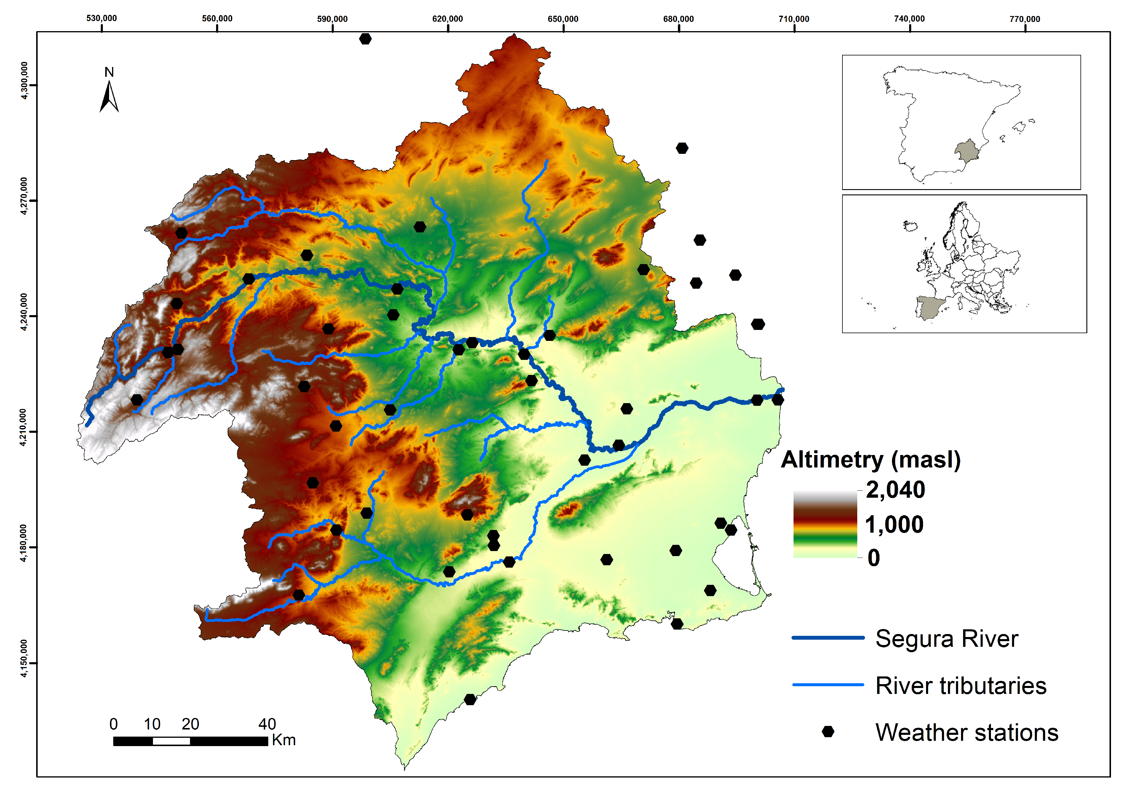
The Segura Hydrographic Demarcation (DHS) (Figure 1) is located in the southeast of the Iberian Peninsula. It has an emerged area of 19,025 km${}^2$ with a large orographic variability, alternating mountain systems that exceed 2000 m.a.s.l. in altitude, with high plateaus, valleys, and coastal depressions [49].

The spatial distribution of temperature is strongly influenced by the orography, with an increase in the average annual temperature from the Northwest mountains ($10{}^{\circ }\mathrm{C}$) to the coast ($18{}^{\circ }\mathrm{C}$). The annual temperature regime presents a winter minimum in the months of December and January, while the maximums correspond to the months of July and August [24].

The average annual rainfall in the period 1980/81–2011/12 was 375 mm [24], making it one of the driest regions in continental Europe. The mountain ranges located in the Northwest average annual rainfall slightly higher than 1100 mm. Precipitation drops drastically in a northwest–southeast direction, with average annual precipitation values around 200 mm in the Southwestern coast. Gomariz-Castillo et al. [26] obtained for the period 2003–2014 an average ET${}_0$ of 1258 mm × year${}^{-1}$, ranging in most of the DHS between 1200 mm and 1300 mm without a clear spatial pattern.

The climate shows great spatial contrasts and a great interannual variability, with relatively frequent torrential events, interannual droughts, heavy frosts, and maximum temperatures that locally can surpass $40{}^{\circ }\mathrm{C}$. Its location and spatial heterogeneity makes it an ideal case study to evaluate the impact of CC in strongly anthropized semi-arid areas of the Mediterranean.

The combination of factors favorable to agriculture (high solar radiation and mild temperatures) allowed the development throughout the twentieth century of a very productive agriculture comparing with the rest of Spain [50]. However, due to the aridity of the DHS and the high water deficit 400 hm${}^3$/year agriculture is highly dependent on irrigation, which has required a large degree of regulation [51], the transfer of water from neighboring areas (the most important being the Tagus–Segura transfer [52]) and the overexploitation of aquifers [45,53]. This overexploitation, together with the decrease in snowfall, due to the increase in temperature related to CC, has meant that 46% of the springs existing in 1916 in the Segura basin have now disappeared [54].

The IPCC-AR5 RCP4.5 scenario [7] estimates a stabilization of temperature increases for the second half of the 21st century, around 1.5 ${}^{\circ }\mathrm{C}$ with respect to the reference period 1961–1990. On the other hand, the RCP8.5 scenario estimates a significant increase in global temperatures of around 3 to 5 ${}^{\circ }\mathrm{C}$ at the end of the 21st century with respect to the period 1961–1990. As a result, in addition to the increase in the ET${}_0$, significant reductions in precipitation are expected, together with an increase in adverse phenomena such as floods and the intensification of droughts, which will cause significant alterations in water availability both in the DHS and in inter-basin transfers [55].

3.2. Data Sources

Three CC scenarios were used: HISTORICAL, ET${}_0$ for the period 1970–2000, and the IPCC-AR5 [6] RCP4.5 and RCP8.5 scenarios for the period 2020–2099. It is thus possible to compare the CC impact on the variable studied with respect to the first scenario. RCP4.5 and RCP8.5 cover time series of emissions and concentrations of the full range of greenhouse gases (GHGs), aerosols and chemically active gases, as well as land use and land cover [6]. RCP4.5 is an intermediate emissions scenario, which estimates a stabilization of GHG emissions from 2050; RCP8.5 is a high GHG emissions scenario, which considers a significant increase throughout the 21st century.

We tried to maximize reproducibility implementing the process described in the methodology in R-CRAN [56], an Open Source program for data analysis that can handle and analyze large volumes of information, and that has a large number of packages available to different types of the calculations. Therefore, it can be applied to one or more time series (one or more weather stations) and for different datasets. The Open Data series of the AEMET [7], regionalized for the Iberian Peninsula with more than 2500 weather stations, are used as a starting point.

AEMET regionalized projections of 16 models (

Table 1. Individual global climate models used in this study, named according to the CMIP5 (Coupled Model Intercomparison) project. Marks indicate the availability of the model in each of the studied scenarios. Last column indicate which models were used for the multi-model ensembles (MMEs) in this study.

Regionalized Model	HISTORICAL Scenario	RCP4.5 Scenario	RCP8.5 Scenario	Model Used for Ensemble
ACCESS1_0 [57]	x	x	x	x
ACCESS1_3 [57]	x		x
bcc_csm1_1 [58]	x	x	x	x
bcc_csm1_1_m [58]	x	x
BNU_ESM [59]	x	x	x	x
CMCC_CESM [60]	x		x
CMCC_CM [61]	x		x
CMCC_CMS [62]	x
CNRM_CM5 [63]	x	x	x	x
inmcm4 [64]	x	x	x	x
IPSL_CM5A_MR [65]	x	x
MIROC_ESM [66]	x	x	x	x
MIROC5 [66]	x	x	x	x
MPI_ESM_LR [67]	x	x	x	x
MPI_ESM_MR [67]	x	x	x	x
MRI_CGCM3 [68]	x	x	x	x
TOTAL	16	12	13	10

) were used to estimate daily ET${}_0$ and to generate the ensembles. Such projections were carried out within the framework of the PNACC, whose objective was, among others, to generate daily series of maximum and minimum temperatures and precipitation, considering local factors in such estimation. To this end, they generated daily series associated with the network of AEMET weather stations based on a regionalization using the statistical method of analogs from the global models participating in the IPCC-AR5 [6] and the project Coordinated Regional Downscaling EXperiment (CORDEX) [2]. The analogs method we used to obtain the series is described in [5]. It is based on the search for historical synoptic situations similar to the days that are regionalized. Its advantage is that, when using time patterns, it keeps the spatial covariance structure of local time, and does not make assumptions about the shape of the probability distribution of the variables. Amblar Francés et al. [5] carry out such regionalization using the following process: (a) to obtain a synoptic classification of atmospheric situations, estimating their similarity using Euclidean distance, and (b) to use as temperature at 2 m, temperatures at three pressure levels (850, 700, and 500 hPa), the zonal and meridian components of the wind at sea level, the pressure at sea level, the temperature at 2 m of the previous day, the specific humidity at 700 hPa and the insolation as predictors.

To apply the study to the DHS, maximum and minimum temperature data associated to 48 weather stations of the AEMET network have been used (Figure 1). The emission scenarios selected in this work are those defined in the IPCC-AR5 for intermediate emissions (Representative Concentration Pathway 4.5-RCP4.5) and high emissions (RCP8.5) [6] for the period 2020–2099.

As can be seen in Table 1, 16 regionalized models are available, although this number is not the same for RCP4.5 and RCP8.5; therefore, to simplify the process, the 16 regionalized models have been evaluated with respect to the observed data, but the MMEs have been generated for the 10 regionalized models available in both RCP scenarios (10 in total).

A third historical scenario is also included with daily data for the period 1961–2000 (HISTORICAL scenario). This scenario includes the series of the previous regionalized models and a series of observed data for that period, used to evaluate goodness of fit and to generate the MME models. For this purpose we used data from the data set Iberia01 [69] that has daily rainfall and temperature series for the Iberian Peninsula obtained from the interpolation of 3486 weather stations (including the weather stations used in this study). The advantage of this type of data over the observed data is that anomalous values and inhomogeneities are removed and the data are spatially distributed in a grid with a resolution of about 12 km.

The series of ET${}_0$ were estimated from the maximum and minimum daily temperature data associated to each of the 16 models. A total of 16 regionalized models (Table 1) × 3 scenarios (HISTORICAL, RCP4.5, and RCP8.5) × 48 stations (Figure 1) = 2304 ET${}_0$ daily temporal series. In addition 48 data series were estimated from historical weather station data series (1961–2000). The Hargreaves equation was used for this estimation.

To train and validate the MMEs, the ET${}_0$ series of the HISTORICAL scenario was divided into a training dataset (1 January 1961 to 31 August 1987) and a test dataset (1 September 1987 to 31 December 2000). As the main objective of this study is the estimation of the future series, the last period was selected for validation. The ET${}_0$ series estimated from the daily maximum and minimum temperature obtained in Spain02v5 was used as reference series.

3.3. Multi-Model Ensemble

Eleven MME methods to combine forecasts of individual regionalized models were analyzed: three simple ensembles, four regression-based ensembles, two geometric-based ensembles, and two machine learning (ML) based ensembles. Simple ensembles, regression-based ensembles, and geometric-based ensembles are implemented in the R package GeomComb [70]. Bayesian Model Averaging (BMA) analysis in the R package BMS [71]. Random Forest (RF) and Support Vector Regression (SVR) in the R packages Random Forest [72] and kernlab [73], respectively. The parameter calibration of the last two methods was carried out using the R package caret [74]. Detailed descriptions of the algorithms are available in the previous references.

The simple ensembles used were Simple Average forecast combination (SA), Median forecast combination (MED), more robust to outliers than SA [75], and Trimmed Average forecast combination (TA). This last method uses a trim factor to eliminate a percentage of the extreme data on both sides of the distribution, being less sensitive to sampling outliers and asymetric distributions than SA [76]. In this study, the trim factor has been estimated by minimizing the RMSE of the predictions with respect to the training data-set.

Regression-based ensembles and geometric-based ensembles are also linear combinations of the members of the ensemble but the weights are optimal in terms of a risk function. Ordinary Least Squares (OLS) regression, first used to build ensembles in Granger and Ramanathan [77], uses ordinary least squares to estimate both the weights and an intercept:

$${\widehat{y}}_t=b_0+\sum _{i=1}^N{f}_{it}\times w_i^{OLS}$$

(3)

where $f_{it}$ is the value of the ensemble member or predictor i at time t; $b_0$ is the intercept, which acts as a bias correction; and $w_i^{OLS}$ is the weight assigned to predictor i. Constrained Least Squares (CLS) forecast combination [77] is conceptually similar to OLS (Equation (3)), but subject to ${\sum }_{i=1}^N{w}_i^{CLS}=1$ and $b_0=0$. It s main advantage over OLS is that CLS produces better estimations when the predictors are highly correlated but, having no $b_0$, it does not correct bias. Least Absolute Deviation (LAD) [78] is another lineal regression-based method (equal to Equation (3)) but $w_i^{LAD\left(N\right)}$ are estimated by minimizing absolute errors instead of squared errors, as in OLS, for this reason it is more robust if outliers are present.

Bayesian Model Averaging (BMA) [79,80] produces a weighted average of probability density functions (PDFs), combining the models while calibrating the weights from the training data set. In this method, the weights are estimated using the posterior probability of each of the individual members. It is a relatively new approach with two main advantages [80,81]: (a) the estimation of weights based on a statistical a priori analysis may ensure objectivity and (b) the idea of assigning higher weights to forecasts that provide unique information is consistent with the recommendation of combining forecasts that incorporate diverse information [76]. This is because systematic and random errors of individual forecasts are more likely to cancel out in the ensemble if the individual forecasts convey different information. Hinne et al. [82] provides a detailed description of its general framework and practical utility, and Wang et al. [20] applies it to CC scenarios.

Standard eigenvector (EIG1) and bias-correct eigenvector (EGI2) proposed in Hsiao and Wan [83] are the two geometric ensembles included in this study. Both estimate the linear combination weights from the sample mean squared prediction error (MSPE) matrix. The main difference among them is that EIG2 uses the centered MSPE matrix [70]; therefore, EIG2 is more advisable if any of the components of the combination is skewed.

Random Forest (RF) and Support Vector Regression (SVR) are the two machine learning approaches tested in this study. Both algorithms are fully explained in Hastie et al. [84] or Kuhn and Johnson [74] and its application to MMEs with CMIP5 data problem is presented in Wang et al. [20].

RF is a nonparametric algorithm that builds an ensemble of decision trees [85]. Each tree is calibrated using a bootstrapped subsample of cases, and the features to perform each split in the trees are selected from a random subsample of the whole feature set. When all trees have been trained, without pruning, each new case is analyzed by all trees and the final prediction is obtained averaging the results. RF uses two parameters: number of regression trees ($n_{tree}$) to grow, and number of features randomly sampled in each split ($m_{try}$). Once the model is trained, the prediction can be obtained as

$${\widehat{y}}_t=\frac{1}{M}\sum _{m=1}^M{T}_m\left(f_t\right)$$

(4)

where M is the number of trees, $T_m$ denotes single decision tree, and $f_t$ is a vector of predictors.

In this study, $n_{tree}=1000$, as higher values do not generally produce any improvement [72,84] and $m_{try}$ has been calibrated using cross validation without repetition and minimizing RMSE. To do this, while saving computing time due to the high number of observations and variables, a cross-validation based on a partition of the training time series by decades in three blocks was carried out. The resulting RMSE values for each block were calculated, and finally the $m_{try}$ value that minimized the average RMSE was selected.

RF importance was estimated using a model-based approach, more related to the actual model performance than the traditional methods, that takes into account the correlation structure between the predictors [74]. The metric used is based on the estimation of MSE on the out-of-bag data for each tree, and then the same computed after permuting a variable. The differences are averaged and normalized by the standard error. Once done, the values obtained have been rescaled to percentages in order to compare the results between the various estimated models. In this way, it is possible to evaluate the contribution of each series to the final ensemble and to determinate which of them are more important in the forecast.

SVR [86] is an extension of Support Vector Machines (SVM) for regression problems. Instead of minimizing the sum of squared errors, it selects points, the so-called support vectors, whose residual absolute values $\left|e\right|$ are larger than a threshold $ϵ$. These points will contribute linearly, instead of quadratically, to the objective error function to be minimized. The problem is then solved as a quadratic optimization problem. A regularization parameter C penalizes large residuals. SVR is generalized to nonlinear regression problems by including in the formulation the so-called kernel functions. In this way, the prediction of ET${}_0$ can be obtained from the following general formulation,

$${\widehat{y}}_t=b_0+\sum _{i=1}^N({\alpha }_i-{\alpha }_i^{*})K(x_k,x)$$

(5)

where $K(X_n,X)$ is the kernel function. In this study a radial basis function (RBF) was used as kernel function.

SVR with the RBF kernel requires setting two parameters: C, the cost parameter, and $\gamma$, a parameter of the RBF kernel function that controls the degree of nonlinearity of the model. To reduce the computational cost, $\gamma$ has been estimated automatically from the training data, following the methodology in Caputo et al. [87], as advised by authors such as Kuhn and Johnson [74]; after that, C has been calibrated from cross-validation, following the same procedure as for RF. Values of $\gamma$ close to 0 produce similar results to the linear model (they reduce the degree of nonlinearity). A large C produces a more flexible but also more likely to overfit [74].

3.4. Evaluation and Comparison of Individual Regional Models and Multi-Model Ensembles

Three statistics were used to estimate error validation: R-squared (R${}^2$), bias percentage (PBIAS), to measure the mean tendency of a model to overestimate or infra-estimate ET${}_0$, and Kling–Gupta efficiency (KGE) that summarizes several aspects of the model performance in fitting reference data.

R${}^2$ can be interpreted as the proportion of the variance of the reference variable reproduced by the simulation. It is defined as

$$R^2=\frac{{\displaystyle \sum _{i=1}^n}{\left(re{f}_i-si{m}_i\right)}^2}{{\displaystyle \sum _{i=1}^n}{\left(re{f}_i-\overline{ref}\right)}^2}$$

(6)

where $si{m}_i$ and $re{f}_i$ are the ET${}_0$ (mm day${}^{-1}$) simulated by a specific model and the reference value, respectively, on a given day, and $\overline{ref}$ is the arithmetic mean of the reference values. Although it is the most widely used fitting statistic, it is very sensitivity to extreme values [88] and insensitive to constant biases (additive or multiplicative).

PBIAS (bias percentage) measures the average tendency of the simulated data to be larger or smaller than their reference values [89]. It is defined as

$$PBIAS=\frac{{\displaystyle \sum _{i=1}^n}\left(re{f}_i-si{m}_i\right)}{{\displaystyle \sum _{i=1}^n}\left(si{m}_i\right)}\times 100$$

(7)

Positive values indicate underestimation bias and negative values indicate overestimation bias [89].

KGE [90] is increasingly being used in calibration and validation studies due to its advantages over other metrics: it normalizes model performance into an interpretable scale and addresses deficiencies of other metrics (as the Nash–Sutcliffe efficiency and $R^2$) due to its formulation [90], summarizes correlation, bias and variability. In this study, we used the modified version proposed in Kling et al. [91] that ensures the no correlation of bias and variability ratios:

$$KGE=1-\sqrt{{\left(r-1\right)}^2+{\left(\frac{C{V}_{sim}}{C{V}_{ref}}-1\right)}^2+{\left(\frac{{\mu }_{sim}}{{\mu }_{ref}}-1\right)}^2}$$

(8)

where r is the lineal correlation between simulated and reference values; $C{V}_{sim}$ and $C{V}_{ref}$ are the coefficients of variation in simulated values and reference values (variability ratio in equation), respectively; and ${\mu }_{sim}$ and ${\mu }_{ref}$ are the mean in simulated values and reference values (bias ratio in equation). Its interpretation is similar to R${}^2$, KGE ranges from -Inf to 1; KGE = 1 indicates perfect agreement between simulations and observations [90].

Two one-way ANOVA tests were performed on the three goodness of fit statistics estimated with the test data-set to identify any statistically significant differences in the individual regionalized models and MMEs. The mean values of each statistic were compared using the observations in the 48 weather stations:

• ANOVA 1. Its objective is to evaluate performance between the different series and forecast methods (Series factor). This variable factor consists of $k=27$ classes (16 regionalized models, 3 simple ensembles, 2 geometric-based ensembles, 4 regression-based ensembles, and 2 machine learning ensembles) and $n=k·48$ stations $=1296$ observations.
• ANOVA 2. In addition, to better interpret the results, a second analysis was designed, with the same data but grouping the series according to their type (regionalized models, simple ensembles, regression-based ensembles, geometric ensembles, and machine learning ensembles).

When the existence of an effect is discovered using ANOVA, the effects and significance of differences between the different models are evaluated with multiple pair contrasts based on a Tukey–Kramer contrast. Such contrasts allow to find homogeneous groups of classes. To evaluate the statistical asssumptions of ANOVA models (normality and homoscedasticity), we used the Kolmogorov–Smirnov test to evaluate normality and the Levene test [92] to evaluate homoscedasticity in the residuals. KS was not significant, but the significance of the Levene contrasts revealed heteroscedasticity. In this case, the covariance matrix of the estimated parameters is not robust enough, and the Tukey–Kramer contrast is less reliable. To correct the heteroscedasticity we used a heteroscedasticity-consistent covariance matrix of the parameters (HC3) [93] in ANOVA and the Tukey–Kramer contrast.

3.5. Temporal and Spatial Patterns of ET${}_0$

In addition to obtaining daily series of ET${}_0$, the spatio-temporal characterization of the CC impact on ET${}_0$ has been carried out by an analysis of the yearly ET${}_0$ in the HISTORICAL scenario and in the RF estimations in the RCP4.5 and RCP8.5 scenarios, as RF resulted to be the most accurate method.

The temporal trend of the annual ET${}_0$ and its significance have been calculated for the average series of all 48 weather stations included in the study. This trend has been estimated using a robust regression based on the Theil–Sen estimator [94] and its significance with Mann–Kendall trend test. These are non-parametric methods with great robustness if statistical assumptions, such as time dependence, are not met [95]. The Theil–Sen estimator is a generalized-based median method that fits a regression line by choosing the median of the slopes of all lines through pairs of points as slope estimation (${\beta }_1$); the sign of ${\beta }_1$ represents the direction of change and its value indicates the steepness of change [96]. Mann–Kendall monotonic trend test [97] is based on the correlation between the ranks of a time series and their time order.

In order to analyze the spatial distribution of the expected changes of annual ET${}_0$, average values of ET${}_0$ at annual scale were obtained for the 48 stations included in the study area for the period 1971–2000, used as reference period, and for the periods 2041–2070 and 2071–2100. These annual values were then interpolated for both periods using Regression Kriging, a technique that combines a global regression model to establish the relation between the dependent variable and different predictors with a local interpolation of its residuals using, in this case, ordinary kriging. Due to the good results obtained in previous works [26] Random Forest was used as the regression model.

Seven geographical variables were initially to be used as predictors for RF: (1) elevation above sea level (m), using a DEM with resolution of 25 m (DTM25) [98]; (2) Euclidean distance to the coast (m) (COASTDIST); (3) mean annual potential irradiation (W/m${}^2$ year${}^1$) (POTI), obtained according to the methodology proposed in Hofierka and Suri [99]; the (4) inverse and (5) logarithmic transformation of the elevation; and the (6) inverse and (7) logarithmic transformation of distance to the coast. These variables can act as proxies for some of the meteorological variables relevant in the calculation of ET${}_0$ but not included in Hargreaves’ equation. For example, POTI is a proxy of the global radiation; DTM25 is a proxy of the ratio of atmospheric pressure to atmospheric pressure at sea level or of wind magnitude, while COASTDIST acts as a proxy of the ratio $T/DeltaT$, humidity, or cloudiness [26].

The multicollinearity between predictors was evaluated using the variance inflation factor (VIF), eliminating in an iterative manner the variables with a threshold greater than 10, as proposed in Kutner et al. [100]. After performing the VIF, the logarithmic transformation of elevation and distance to the coast were eliminated due to high collinearity, so the final number of variables used as predictors was 5.

Once the spatial distribution of the annual ET${}_0$ of the three scenarios was obtained, the differences were evaluated for significance using ANOVA and a posteriori contrasts described in Section 3.4.

3.6. Summarized Workflow

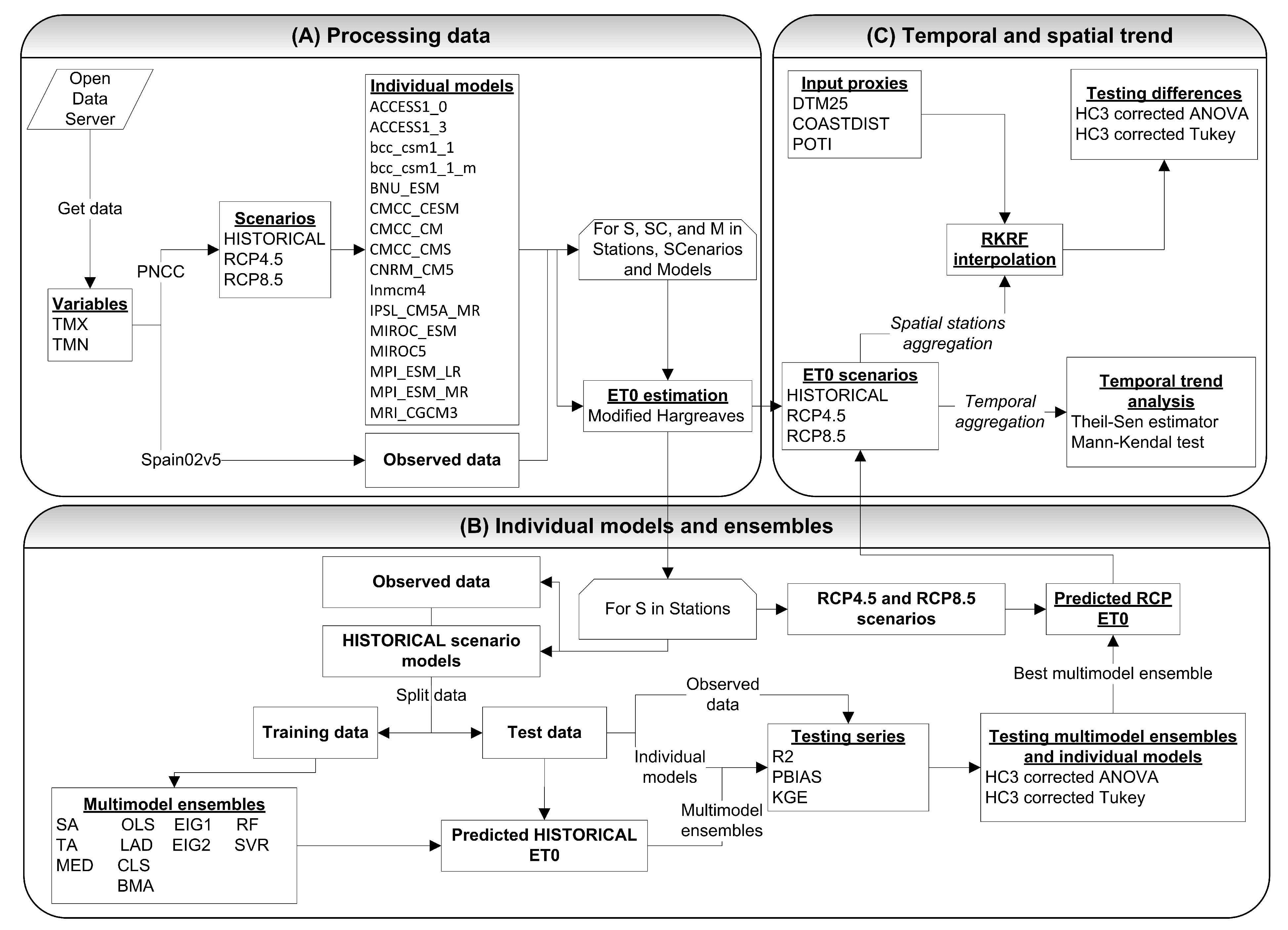
The conceptual scheme in Figure 2 summarizes the calculation process. A sample code for a weather station is included as Supplementary Materials. It computes (a) the estimation of ET${}_0$ from the daily maximum and minimum temperatures associated with the individual regionalized models, (b) the validation of the individual regionalized models and the multi-ensemble models, and (c) the predictions for the RCP scenarios. The processes and code use are described in the file README.pdf, included in the Supplementary Materials.

Figure 2A shows the downloading and preprocessing steps, described in Section 3.2. The maximum and minimum daily temperatures (TMX and TMN) of the weather stations included in the study area are downloaded and processed for the three considered scenarios and the 16 individual regionalized models; in addition, the observed data are downloaded and processed. Then, for each station, scenario and model (including the observed data), the ET${}_0$ is obtained using the Hargreaves calibrated equation (see Section 2).

Once all the series of ET${}_0$ are obtained, as summarized in Figure 2B, we start with the estimation of the 11 MMEs in an iterative way for each station (48) in the HISTORICAL scenario (see Section 3.3). For this purpose, 2/3 of the data series was used to fit the models (train data, from 1961 to 1987), and 1/3 as test data (from 1988 to 2000). Additionally, for the machine learning algorithms, a cross-validation is performed to obtain validation data in each K iteration. Once the MMEs are estimated, they are validated and the validation results compared (see Section 3.4) using one-way ANOVA and Tukey–Kramer post hoc tests using HC3 heterocedasticity correction. After that, the method that best fits the observed values is selected and the predicted series are generated from that method.

Finally, Figure 2C summarizes the characterization of the hypothetical impact of CC on the temporal and spatial ET${}_0$ patterns in the study area. On the one hand, the Theil–Sen and Mann–Kendal regression is used to analyze the ET${}_0$ trend (mm year${}^{-1}$) in the three scenarios, obtaining the average annual increase in each of them.

For the spatial characterization, a spatial interpolation based on Random Forest Regression Kriging of mean ET${}_0$ values (mm year${}^{-1}$) is carried out, comparing the differences of the predicted values in the interpolation surface of the RCP4.5 and RCP8.5 scenarios (for the annual mean values of the periods 2041–2070 and 2071–2099) with respect to the reference HISTORICAL scenario (annual mean values of the period 1971–2000). To estimate whether the differences are significant, the same methods are used as in the previous case.

4. Results and Discussion

4.1. Performance of Individual Models and Multi-Model Ensembles

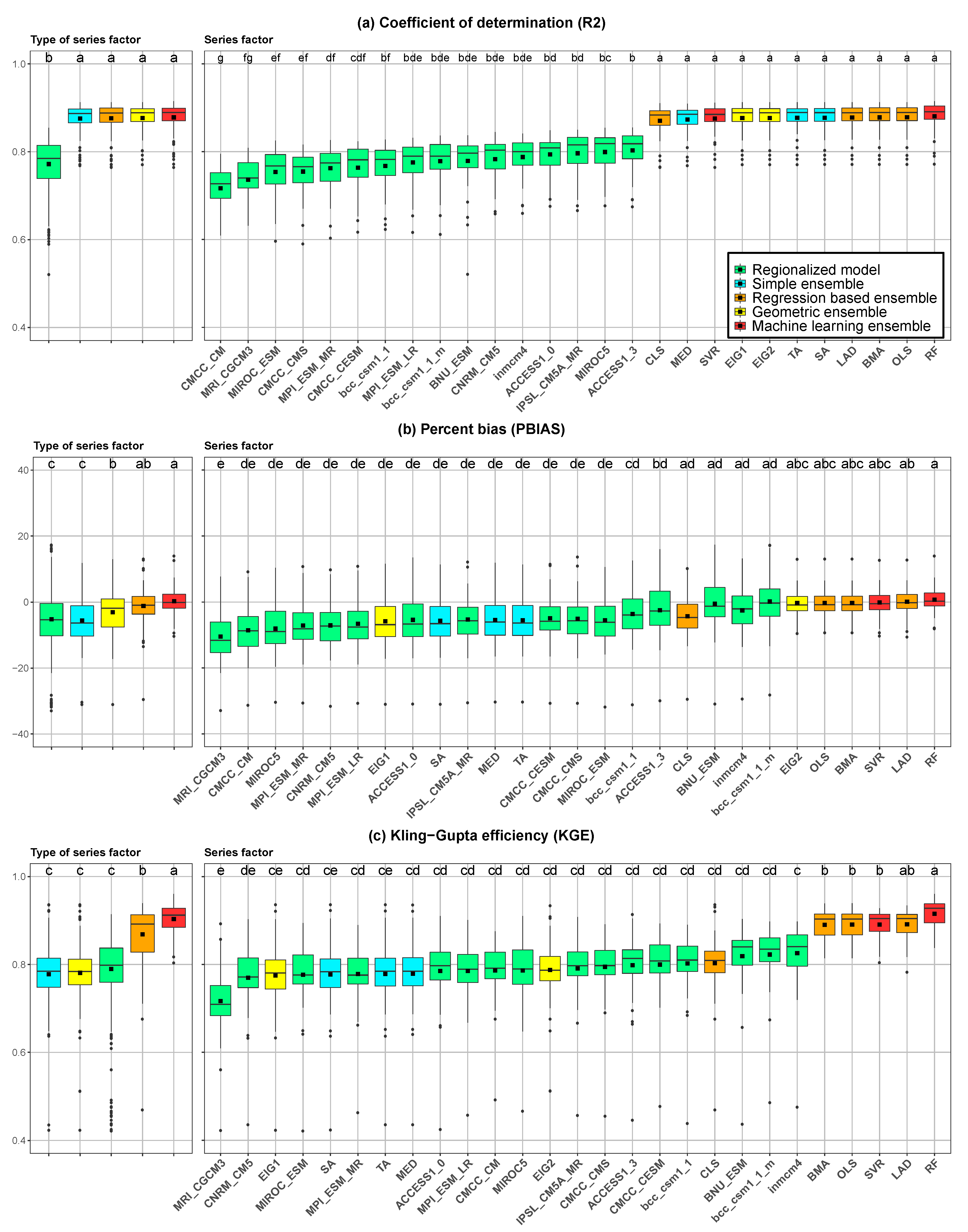
The ANOVA analyses performed on the goodness-of-fit statistics of MMEs and regionalized models show significant differences in the three analyzed statistics, both when each series is considered separately ($F(26,1269)$, $p<0.0001$ in all three cases) and when the series are aggregated by type ($F(4,1291)$, $p<0.0001$ in all three cases). Figure 3 shows the value distribution of such statistics, and also the groupings obtained with the Tukey–Kramer post hoc test.

Table A1. Goodness of fit statistics in calibration for the different series. $N=1296$ observations ($n_k=48$ weather stations by class).

Type of Serie	Series Class	R${}^2$	sd	se	PBIAS (abs.)	sd	se	KGE	sd	se
Regionalized individual model	ACCESS1_0	0.779	0.041	0.006	6.22	5.23	0.76	0.803	0.078	0.011
	ACCESS1_3	0.795	0.043	0.006	4.83	5.10	0.74	0.802	0.076	0.011
	bcc_csm1_1	0.757	0.046	0.007	6.79	5.24	0.76	0.784	0.075	0.011
	bcc_csm1_1_m	0.785	0.044	0.006	5.56	5.24	0.76	0.839	0.067	0.010
	BNU_ESM	0.774	0.051	0.007	5.05	5.16	0.74	0.827	0.071	0.010
	CMCC_CESM	0.762	0.049	0.007	6.05	5.47	0.79	0.816	0.073	0.010
	CMCC_CM	0.779	0.039	0.006	7.13	5.28	0.76	0.813	0.070	0.010
	CMCC_CMS	0.762	0.042	0.006	6.28	5.32	0.77	0.816	0.072	0.010
	CNRM_CM5	0.775	0.046	0.007	7.99	5.53	0.80	0.784	0.078	0.011
	inmcm4	0.783	0.042	0.006	5.08	5.17	0.75	0.833	0.070	0.010
	IPSL_CM5A_MR	0.784	0.043	0.006	6.89	5.53	0.80	0.791	0.074	0.011
	MIROC_ESM	0.762	0.051	0.007	6.58	5.51	0.80	0.786	0.082	0.012
	MIROC5	0.788	0.042	0.006	8.81	5.40	0.78	0.789	0.077	0.011
	MPI_ESM_LR	0.769	0.046	0.007	7.45	5.54	0.80	0.799	0.076	0.011
	MPI_ESM_MR	0.763	0.048	0.007	7.59	5.47	0.79	0.794	0.075	0.011
	MRI_CGCM3	0.733	0.047	0.007	9.74	5.71	0.82	0.731	0.079	0.011
Geometric based ensemble	EIG1	0.871	0.027	0.004	6.88	5.36	0.77	0.784	0.084	0.012
	EIG2	0.871	0.027	0.004	0.00	0.00	0.00	0.798	0.073	0.010
Machine learning based ensemble	RF	0.974	0.005	0.001	1.12	0.41	0.06	0.957	0.010	0.001
	SVR	0.904	0.022	0.003	0.38	0.24	0.03	0.926	0.019	0.003
Regression based ensemble	BMA	0.872	0.027	0.004	0.00	0.00	0.00	0.906	0.020	0.003
	CLS	0.864	0.031	0.004	5.00	4.66	0.67	0.815	0.072	0.010
	LAD	0.872	0.027	0.004	0.61	0.49	0.07	0.906	0.023	0.003
	OLS	0.872	0.027	0.004	0.00	0.00	0.00	0.907	0.020	0.003
Simple ensemble	MED	0.867	0.027	0.004	6.51	5.22	0.75	0.789	0.082	0.012
	SA	0.871	0.027	0.004	6.71	5.34	0.77	0.787	0.083	0.012
	TA	0.871	0.027	0.004	6.53	5.22	0.75	0.788	0.082	0.012

and

Table A2. Goodness of fit statistics in validation for the different series. $N=1296$ observations ($n_k=48$ weather stations by class).

Type of Serie	Series Class	R${}^2$	sd	se	PBIAS (abs.)	sd	se	KGE	sd	se
Regionalized model	ACCESS1_0	0.794	0.043	0.006	7.61	5.58	0.81	0.785	0.079	0.011
	ACCESS1_3	0.803	0.046	0.007	6.34	5.06	0.73	0.798	0.075	0.011
	bcc_csm1_1	0.768	0.050	0.007	6.45	5.27	0.76	0.802	0.071	0.010
	bcc_csm1_1_m	0.779	0.051	0.007	5.78	5.29	0.76	0.822	0.066	0.010
	BNU_ESM	0.779	0.059	0.009	5.93	5.36	0.77	0.819	0.072	0.010
	CMCC_CESM	0.764	0.053	0.008	7.36	5.11	0.74	0.800	0.068	0.010
	CMCC_CM	0.717	0.044	0.006	9.51	5.99	0.86	0.786	0.063	0.009
	CMCC_CMS	0.755	0.049	0.007	7.36	5.38	0.78	0.794	0.069	0.010
	CNRM_CM5	0.783	0.049	0.007	8.38	5.79	0.84	0.770	0.077	0.011
	inmcm4	0.788	0.046	0.007	5.85	5.14	0.74	0.826	0.068	0.010
	IPSL_CM5A_MR	0.796	0.049	0.007	7.45	5.34	0.77	0.791	0.071	0.010
	MIROC_ESM	0.754	0.053	0.008	7.30	5.56	0.80	0.777	0.075	0.011
	MIROC5	0.799	0.046	0.007	9.34	6.06	0.87	0.786	0.077	0.011
	MPI_ESM_LR	0.775	0.050	0.007	8.20	5.60	0.81	0.785	0.072	0.010
	MPI_ESM_MR	0.762	0.051	0.007	8.59	5.70	0.82	0.778	0.070	0.010
	MRI_CGCM3	0.736	0.048	0.007	11.07	6.40	0.92	0.716	0.083	0.012
Geometric based ensemble	EIG1	0.877	0.033	0.005	7.70	5.56	0.80	0.775	0.082	0.012
	EIG2	0.877	0.033	0.005	3.30	2.92	0.42	0.787	0.069	0.010
Machine learning based ensemble	RF	0.881	0.032	0.005	3.09	3.00	0.43	0.915	0.031	0.004
	SVR	0.875	0.033	0.005	3.25	2.97	0.43	0.891	0.032	0.005
Regression based ensemble	BMA	0.878	0.033	0.005	3.28	2.93	0.42	0.890	0.033	0.005
	CLS	0.870	0.035	0.005	6.18	5.01	0.72	0.803	0.071	0.010
	LAD	0.878	0.033	0.005	3.20	2.98	0.43	0.891	0.035	0.005
	OLS	0.878	0.033	0.005	3.28	2.92	0.42	0.890	0.033	0.005
Simple ensemble	MED	0.873	0.033	0.005	7.41	5.48	0.79	0.779	0.080	0.012
	SA	0.877	0.033	0.005	7.56	5.52	0.80	0.777	0.082	0.012
	TA	0.877	0.033	0.005	7.41	5.46	0.79	0.778	0.080	0.012

show their estimation both in calibration and validation. In general, the regionalized individual models (green boxes in Figure 3) have a good fit to the observed data. Figure 3 shows that R${}^2$ > 0.6 in all weather stations except for one in BNU_ESM, although on average they underestimate ET${}_0$ (negative bias in Figure 3b) except for bcc_csm1_1_m. This may be because the method we used to estimate ET${}_0$, take into account maximum and minimum daily temperatures, which are accurately estimated in their regionalization. Thus, Amblar Frances et al. [5] indicate, when carrying out the regionalization for all Spain, that the cause of the good fit may be that when generating the series, the uncertainty associated with the emissions predominates over those associated with the models and processes of regionalization that were used.

An interesting pattern appears in the correlation coefficient R${}^2$ (Figure 3a): although RF is the best, all MMEs methods are grouped as a (no significant differences are observed between them) including the simple ensembles MMEs; therefore, this statistic does not discriminate adequately the performance of the different methods. Traditionally, this statistic has been used to interpret the goodness of fit, but it may induce errors in the final conclusions (Figure 3b,c). In this case, the problem is that R${}^2$ is insensitive to constant deviations (bias) [88]. Therefore, KGE does a better estimation of the true performance of the series, resulting in the machine learning and regression based ensembles, labeled by the post hoc tests as a to b, as the most accurate estimation method. KGE is a better statistic because it integrates the correlation, the variability and the bias (Equation (8)) [90,91].

In general, MMEs outperformed regionalized individual models, which is in agreement with the rest of the literature on MMEs [20,101]. It is, however, noteworthy that MMEs based on eigenvectors and CLS perform worse in PBIAS and KGE. For the three goodness of fit statistics, machine learning-based ensembles are slightly better than the rest of categories, both RF and SVM are included (Type of series factor) in post hoc group a in KGE (significantly better than the others, $M=0.903$, $SD=0.034$) and PBIAS ($M=3.17$, $SD=2.97$), although in this case regression based ensembles appear in the same post hoc group $ab$ ($M=3.98$, $SD=3.77$), being both significantly better than geometric based ensembles and individual regionalized models.

RF is the best MME in KGE (post hoc group a; $M=0.915$, $SD=0.031$), significantly better than the other MMEs, except LAD (post hoc group $ab$; $M=0.891$, $SD=0.035$), while SVM is grouped in b, along with other ensembles algorithms. The performance of RF in the other statistics is slightly higher than the others ($M=0.881$, $SD=0.032$ in R${}^2$, $M=3.09$ and $SD=3.00$ in $PBIAS$). Besides, it can be seen in Figure 3b that average PBIAS ($M=0.70$, $SD=4.26$) is close to 0, and its dispersion is the smallest. Figure 3c shows a KGE outlier associated to weather station 7117; even in that case, RF is significantly better than the rest of ensembles: KGE around $0.80$ in BMA, OLS, SVR, and LAD, while in RF $KGE=0.847$. Although there are few studies where RF and SVM are used, for the purpose of our work, we can highlight that our results are consistent with those obtained in Wang et al. [20] for monthly temperatures with respect to the other two methods it used (BMA and SA). In our study the RF performance is even better, significantly better than SVM, BMA, or SA, even though we analyzed daily data.

Regression-based MMEs (orange color in Figure 3) also show a good performance. In general, they are not significantly different from SVM; it is noteworthy that, although no significant differences are observed in R${}^2$ and PBIAS with respect to other methods such as geometric or simple ensembles, in KGE it is differentiated from the rest as b category. Its good performance may be because ET${}_0$ estimated in this study is based on temperatures, and as pointed out by authors such as Amblar Frances et al. [5], temperature fields are usually smooth, and their statistical behavior is closer to normal than other variables, so regression methods obtain more accurate results. Among the methods used, LAD obtains slightly better performance probably because it is less sensitive to outliers and more stable, when predictors are highly correlated, than regression based on least square estimations, in which low fluctuations in the sample can cause large changes in the coefficients, producing poor predictive performance [102]. The worst performing method is CLS, which in the case of KGE is outside the b grouping of the post hoc tests. This is because it does not include a parameter $b_0$ acting as a correction of the systematic bias that occurs in the individual regionalized models, as OLS does.

The Eigenvector-based MMEs have a much poorer fit to the observed data than the rest of the MMEs. As pointed out in Hsiao and Wan [83], EIG2 is better than EIG1 due to the high bias in regionalized models. In fact, unlike what happened in Hsiao and Wan [83], EIG2 is significantly different to EIG1 in absolute PBIAS. In addition, this author points out its usefulness over the models based on regression when the performance of the different members are similar, but in our study there are significant differences among them.

Simple methods can be more robust than more complex techniques, due to their simplicity (no need to estimate any parameter or weighting of the members included in the analysis [75,103]) even with a small number of observations or underlying changes in the timeline [104]. That is the reason why they are included in the a post hoc group in Figure 3a. However, PBIAS and KGE values are poorer because they produce large errors when the predictors are biased [103]. Even so, it is interesting to use SA as a baseline with which to compare the outputs of the other methods [105,106]. SA appears in the $cd-ce$ groups of the post hoc tests for KGE; in this case, all MMEs perform better than SA except EIG1. MED and TA slightly better on average in KGE and PBIAS, although without significant differences, probably due to their greater robustness against outliers [75].

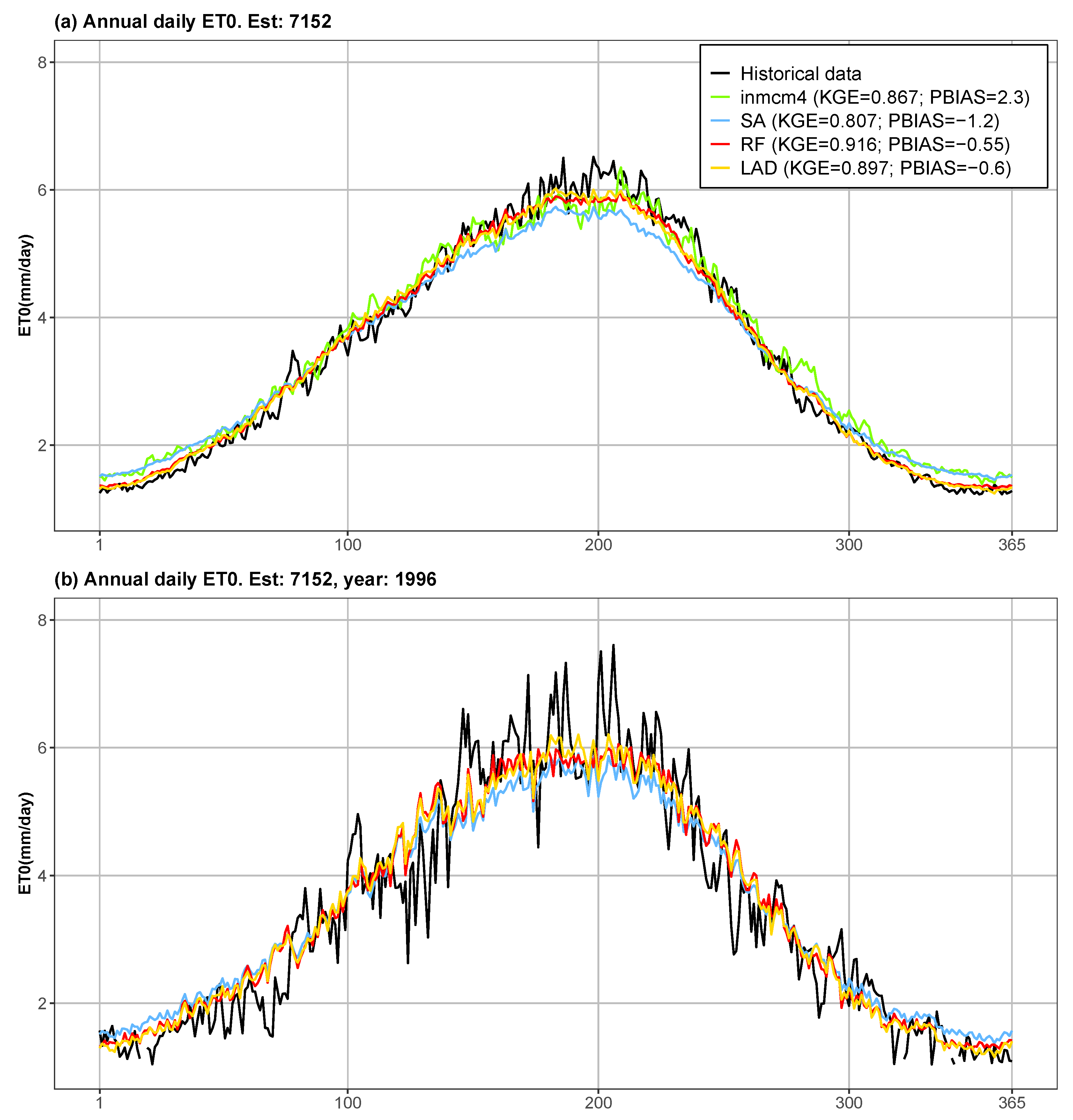
Figure 4 shows, as an example, the prediction of ET${}_0$ (mm day${}^{-1}$) in weather station 7152, located in the center of the DHS. The figure shows a hypothetical year (a), estimated from the average daily values or the test data, and the results for 1996 (b). Its goodness of fit in validation is good and similar to the average values in Figure 3. It includes the forecasts of the two best MMEs (RF and LAD) and SA as a reference series.

The multi-model ensemble methods RF and LAD follow the observed seasonal pattern. In general, the models underestimate the reference series in the months with the highest temperature (and therefore the highest amount of energy) and tend to overestimate it in the colder months. However, the percentage of bias of the whole RF (PBIAS = $-0.55\%$) and LAD (PBIAS = $-0.6\%$) validation series are lower than the rest of the series: in SA PBIAS = $-1.2\%$ and in inmcm4 percent bias is positive (PBIAS = $2.3\%$).

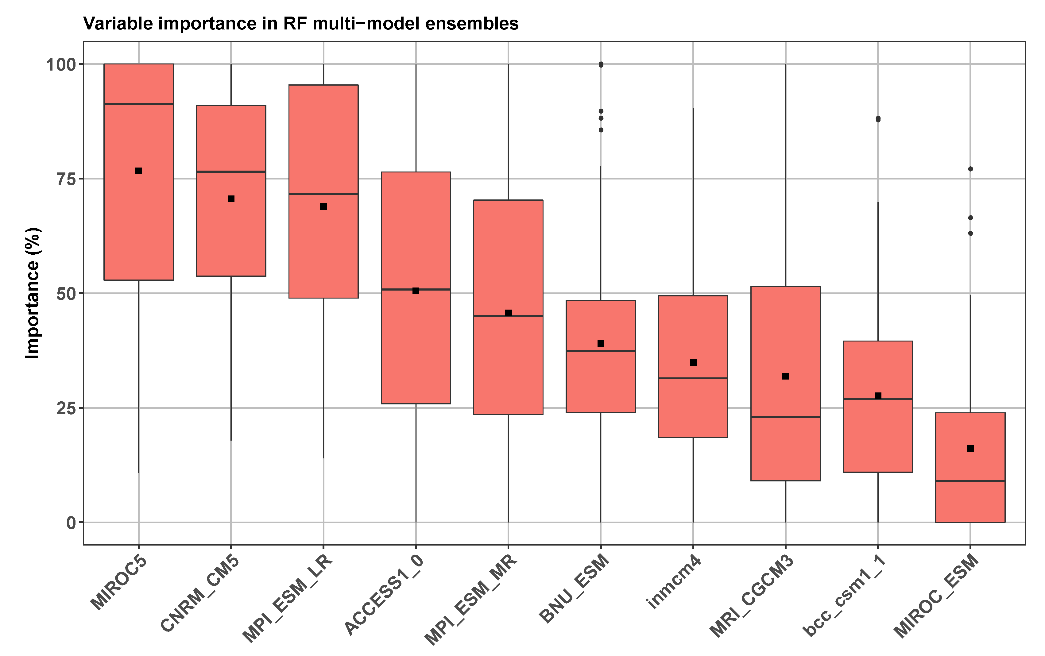
Figure 5 represents the importance of the individual models in the RF ensemble (a summary is included in

Table A3. Averaged relative variable importance in RF ensembles ($n=48$ weather stations).

Regionalized Individual Model	Importance (%)	sd	se
MIROC5	76.67	29.21	4.22
CNRM_CM5	70.57	24.83	3.58
MPI_ESM_LR	68.86	27.28	3.94
ACCESS1_0	50.47	30.41	4.39
MPI_ESM_MR	45.69	30.57	4.41
BNU_ESM	39.04	26.95	3.89
inmcm4	34.81	23.74	3.43
MRI_CGCM3	31.91	27.98	4.04
bcc_csm1_1	27.63	22.56	3.26
MIROC_ESM	16.16	20.33	2.94

); it shows a relatively high dispersion of relative importance, reflecting differences in the behavior of different regionalized individual models depending on the location of weather stations, and therefore possible local effects. The results highlight MIROC5, CNRM_CM5, and MPI_ESM_LR as the most important, with mean relative importance values de 76.67%, 70.57%, y 68.86%, respectively. It is interesting that none of the three stand out for their performance in Figure 3, except MIROC5 and only in R${}^2$, moreover all three have a high negative bias. This behavior may indicate that there are patterns in them that are not contemplated in the rest of the series, and therefore, although are not highly accurate individually, they are useful in the forecasting ensemble.

4.2. Temporal and Spatial Trend of Climate Change Scenarios

4.2.1. Temporal Trend of Anual ET${}_0$

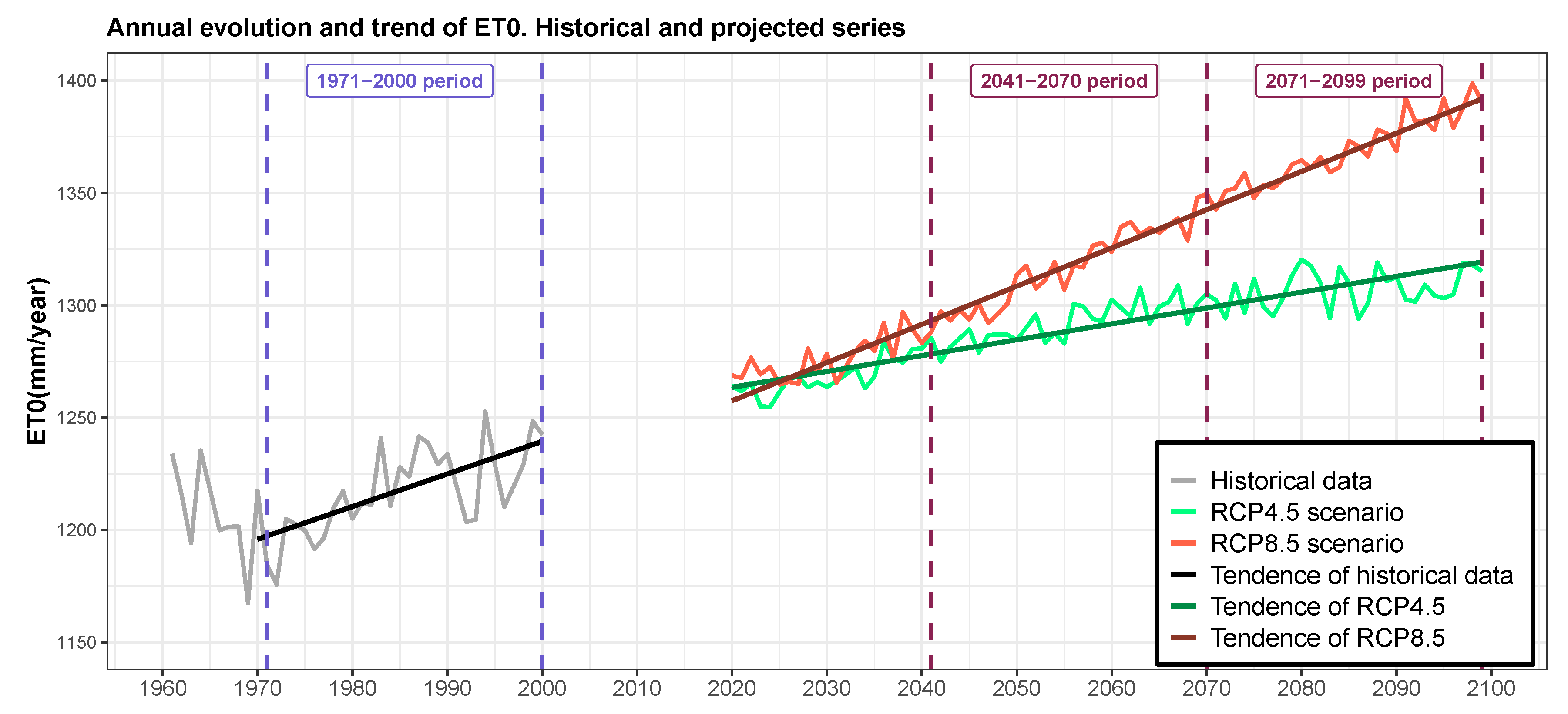
Annual time series during the period 2021–2099 (Figure 6) reveal a statistically significant and positive ET${}_0$ trend (Mann–Kendall tests in

Table 2. The results of the Mann–Kendall test and Theil–Sen regression.

Scenarios	S	Z	p-Value	${\mathrm{fi}}_0$ (mm year${}^{-1}$)	${\mathrm{fi}}_1$ (mm year${}^{-1}$)
HISTORICAL	223	3.773	0.0002	1194.467	1.45
RCP4.5	2370	9.842	>0.0001	1262.78	0.71
RCP8.5	2870	11.920	>0.0001	1255.79	1.70

) in both the HISTORICAL scenario ($Z_{MK}=3.773$, $p=0.0002$) and the two RCP scenarios ($Z_{MK}=9.842$ and $11.920$, $p<$ 0.0001). For the RCP8.5 scenario, a significant increase (1.70 mm/year) is predicted in the ET${}_0$ over the entire 21st century, according with the significant temperature increase predicted for that scenario. For the RCP4.5 scenario, the projected increase of ET${}_0$ is considerably less than that of RCP8.5 (0.71 mm/year). This increase would be mainly concentrated in the first half of the period, followed by an stabilization by the end of the century, as can be seen in Figure 6.

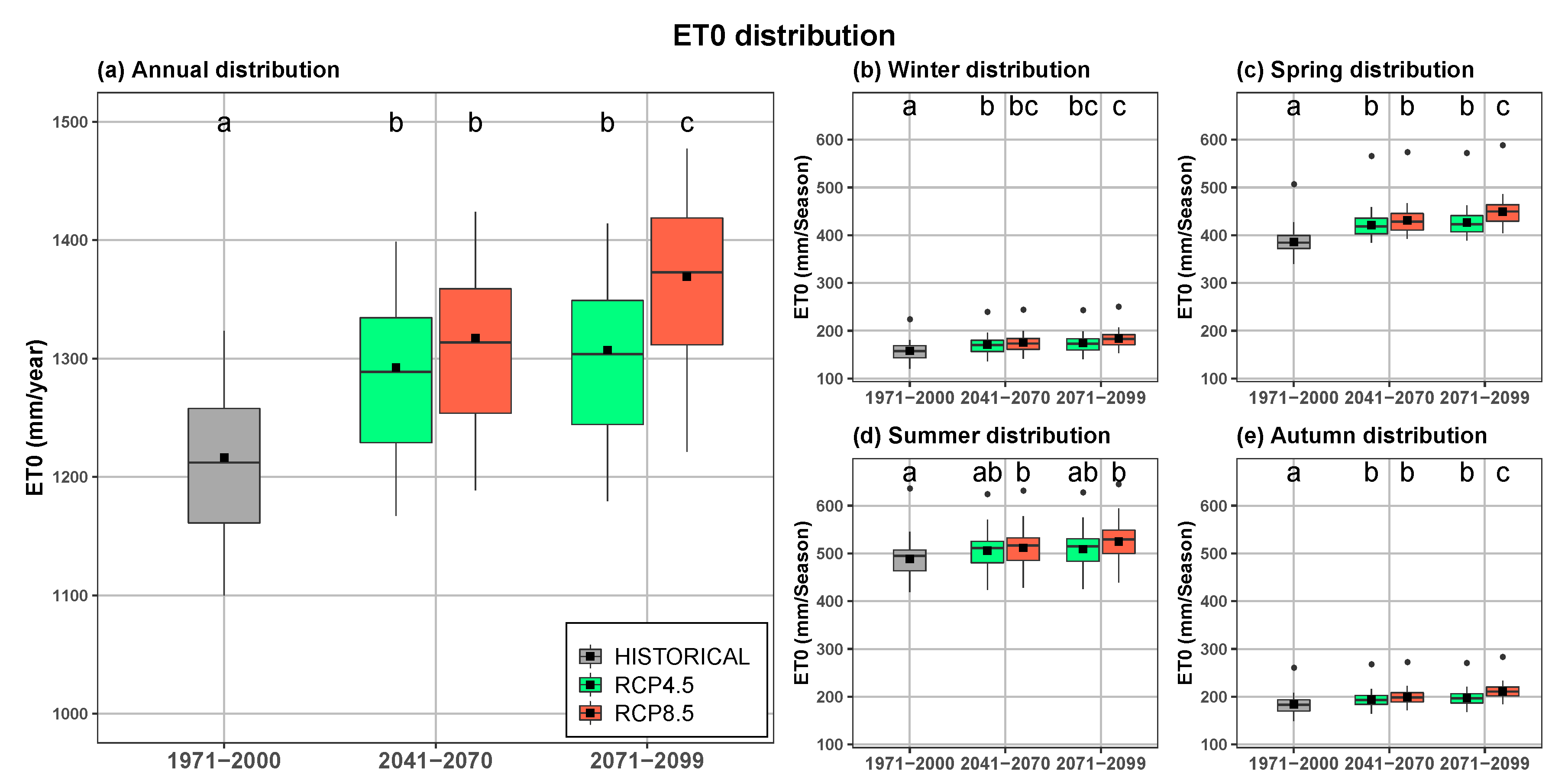
Figure 7 shows the distribution of ET${}_0$ for the historical period and for the two periods contemplated for the RCP4.5 and RCP8.5 scenarios. These distributions are shown at both annual and seasonal scales, and also show the results of the posteriori contrast carried out. The ANOVAs performed for the five situations show significant differences in all cases (Annual: $F(4,235)=19.687$, $p<0.0001$; Summer: $F(4,235)=5.724$, $p<0.0002$; Winter: $F(4,235)=12.802$, $p<0.0001$; Autumn: $F(4,235)=15.257$, $p<0.0001$; Spring: $F(4,235)=30.975$, $p<0.0001$). According to the values obtained for the F statistics in the different seasons, the highest increments of ET${}_0$ are observed for spring, while the lowest variation has been obtained for summer. Tomas-Burguera et al. [107] analyzed the evolution of the ET${}_0$ in Spain for the period 1961–2014, and they also obtain the highest increments of ET${}_0$ for the study area in spring. The results obtained in both works for that season may have or may be already having repercussions in water resources availability, these repercussions should be analyzed in future studies.

With regard to the ex-post contrast carried out to compare the ET${}_0$ distributions obtained for the different periods and scenarios, in all the cases analyzed, with the exception of some cases of summer, there are significant differences between the historical period and the periods corresponding with the two climate change scenarios. In summer, only the ET${}_0$ values obtained for the period 2071–2100 are significantly different from the HISTORICAL scenario, another indication that summer is the season with lowest ET${}_0$ increases. In autumn, differences are not great, although enough for all the scenarios to be significantly different from HISTORICAL; in this case, RCP8.5 for 2071–2099 is significantly different from the rest of the scenarios.

On the other hand, for the RCP4.5 scenario no significant differences have been obtained between both periods in any of the five situations analyzed, which is a consequence of the stabilization of the increase in temperature and therefore of the ET${}_0$ foreseen for that scenario. On the other hand, for the RCP8.5 scenario there are significant differences between both periods for the annual scale as well as for spring and autumn, which agrees with the important and continuous increase of temperature foreseen for the RCP8.5 scenario throughout the 21st century. Furthermore, it should be noted that for the period 2041–2070 none of the five situations analyzed show significant differences between both scenarios. On the other hand, for the period 2071–2100 significant differences have been obtained between both scenarios both on an annual scale and for autumn and spring, which also agrees with the evolution of the estimated temperature for both scenarios.

Table A4. Summary of annual and seasonal ET${}_0$ ($n=48$ weather stations by period and scenario).

	Period	Scenario	ET0 (mm)	sd	se
Annual	1971–2000	HISTORICAL	1216.32	85.44	12.33
	2041–2070	RCP4.5	1292.36	85.08	12.28
	2041–2070	RCP8.5	1317.32	86.10	12.43
	2071–2099	RCP4.5	1307.21	85.76	12.38
	2071–2099	RCP8.5	1369.13	88.57	12.78
Autumn	1971–2000	HISTORICAL	184.24	18.76	2.71
	2041–2070	RCP4.5	194.20	16.99	2.45
	2041–2070	RCP8.5	199.71	16.78	2.42
	2071–2099	RCP4.5	197.49	16.98	2.45
	2071–2099	RCP8.5	211.13	16.52	2.39
Spring	1971–2000	HISTORICAL	385.87	27.26	3.93
	2041–2070	RCP4.5	421.51	29.21	4.22
	2041–2070	RCP8.5	430.92	29.20	4.21
	2071–2099	RCP4.5	426.63	29.37	4.24
	2071–2099	RCP8.5	449.52	29.54	4.26
Summer	1971–2000	HISTORICAL	488.43	35.83	5.17
	2041–2070	RCP4.5	505.66	37.46	5.41
	2041–2070	RCP8.5	511.65	38.50	5.56
	2071–2099	RCP4.5	509.03	37.95	5.48
	2071–2099	RCP8.5	524.97	40.42	5.83
Winter	1971–2000	HISTORICAL	157.79	18.34	2.65
	2041–2070	RCP4.5	170.99	18.36	2.65
	2041–2070	RCP8.5	175.04	18.17	2.62
	2071–2099	RCP4.5	174.07	18.19	2.63
	2071–2099	RCP8.5	183.51	17.30	2.50

shows the average, the standard deviation and the standard error of ET${}_0$ values for each of the five cases analyzed, both on an annual and on a seasonal scale.

4.2.2. Spatial Distribution of Annual Variation in ET${}_0$

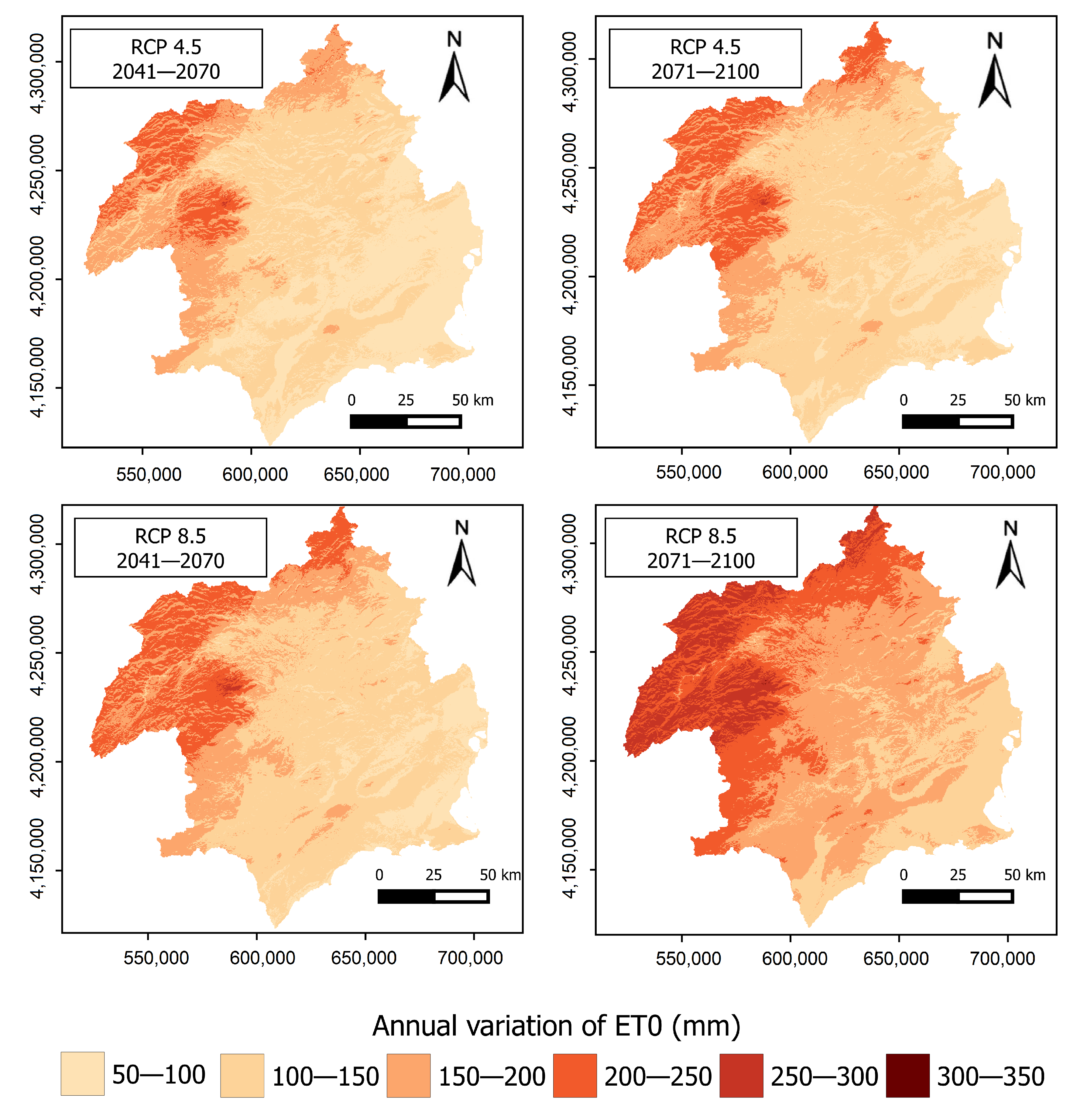
Figure 8 shows the spatial distribution of the ET${}_0$ estimated variation for the two scenarios analyzed in the periods 2041–2070 and 2071–2100 with respect to the reference period. The same spatial pattern exists for the four scenarios represented, with the largest increases of ET${}_0$ in the basin headwaters (northwestern of the study area) and the smallest increases in coastal areas.

For the RCP4.5 scenario, only in the northwest and north end of the study area, an increase larger than 200 mm/year in both analyzed periods is observed. In the rest of the basin the increase ranges between 50 and 200 mm/year. Moreover, for this scenario, hardly any changes are observed between the two analyzed periods, which confirms what was mentioned in previous sections. For the RCP8.5 scenario, the highest increases of ET${}_0$ are estimated in a large area in the northwest of the DHS, especially for the period 2071–2100, with increases larger than 250 mm/year, while the increase exceeds 150 mm in a large part of the DHS. In this case, changes are observed between both periods.

This spatial pattern could mean a decrease in the water resources available in the study area, as most of them are produced in the northwest sector, due to a larger rainfall and permeability of the rocks. Moreover, the outstanding increase of ET${}_0$ observed in the northwestern sector may produce an increase of the evaporation losses in the reservoirs, a reduction of the channel runoff and a reduction of the aquifer recharges. Tomas-Burguera et al. [107] also obtain the largest increases of ET${}_0$ for the period 1961–2014 in the northwest zone of the study area, with a significant increase of 15–30 mm/decade.

Table 3. Comparison of the average variation (%) estimated in the present work and in CEDEX [45] for the entire DHS for the 2 scenarios and the 2 periods used. The variations are referred to the control periods 1961–2000 in CEDEX [45] and 1971–2000 in the case of the present study.

	CEDEX		This Study
Scenario/Impact Period	2041–2070	2071–2100	2041–2070	2071–2100
RCP4.5	6	8	10.7	11.2
RCP8.5	9	15	11.8	15.3

compares the average variation in ET${}_0$ estimated both in this work and in CEDEX [45] for the DHS (as the difference in percentage between the HISTORICAL scenario and the two climate change scenarios and the two periods analyzed in this study). Although the methodology used is not the same in both cases, it shows the similarity between both studies. The variation of estimated ET${}_0$ in this work is greater than the one estimated in CEDEX [45], with the exception of scenario RCP8.5 for the period 2071–2100. The differences between both studies may be due to the different methodologies used to obtain the ET${}_0$ values, to the fact that the data shown for CEDEX [45] are a simple average of the ET${}_0$ variations obtained for six regionalized projections and to the difference in the control periods used, although the influence of the latter would be minimal according to what is observed in Figure 6.

In summary, for the RCP4.5 scenario the estimated ET${}_0$ average increase with respect to the period 1971–2000 is 10.7%, for the period 2041–2070, and 11.8% for the period 2071–2100, while for the RCP8.5 scenario this increase is 11.2% for the period 2041–2070 and 15.3% for the period 2041–2070.

5. Conclusions

Multi-model ensemble methods generally outperform all or almost all individual series. The observed fit in validation, especially considering that the forecasts are have been carried out for a daily time step, justifies the use of this type of method and its usefulness to characterize the climatic variables for different CC scenarios.

We conclude that machine learning MMEs are efficient and highly useful methods, with ability to obtain better predictions, with high precision and better reproduction of historical climatic variables. In our study, RF is salient because of two aspects: (a) its accuracy is significantly better than the rest of individual regionalized series and multi-model ensembles methods, also reducing the bias compared to the rest of the methods, which generally underestimate ET${}_0$ in the warmer months and overestimate it in the colder months, and (b) that RF conveys the different representations of physical processes in individual models, reducing their implicit uncertainty. In addition, RF has several advantages as a predictive model. It is robust to outliers and nonlinear data, produces an estimation of variable importance that allows to weight or select variables, works efficiently with large volumes of data, produces an unbiased estimation of generalization error and is computationally lighter than other machine learning algorithms like SVM. For all these reasons, RF can be useful when analyzing other climate variables, such as precipitation.

However, it is necessary to highlight the importance of using and comparing various methods as model accuracy can differ between variables, climatic zones, or even periods. This paper proposes a framework based on Open Source data analysis software to objectively compare different models and select the most accurate. It can be used with different datasets and study areas, and include other multi-model ensembles, such as REA, inverse Rank, or other machine learning algorithms in futures studies.

Using alternative statistics to evaluate goodness of fit is also useful. Traditionally, R${}^2$ has been used to evaluate correlation, and CC-oriented studies have given special importance to bias. The main advantage of KGE decomposition is that it evaluates, in an integrated way, three fundamental aspects: correlation, variability and bias. In this study, KGE does a better discrimination of the performance of the different ensembles than R${}^2$.

ET${}_0$ trend reveals a statistically significant increase in the three analyzed scenarios, although higher in RCP4.5, where it tends to stabilize towards the second part of the century. This increase, more accentuated in spring, is also observed when carrying out an intra-annual analysis. This trend can cause serious problems in this semi-arid area because of its high water deficit and strong anthropic pressure. The problem might be even exacerbated by the expected reduction in rainfall. The strong water demand by irrigated crops, a large population density, and several touristic resorts increases precisely in the months with a larger increase in ET${}_0$. Moreover, the largest ET${}_0$ increases are expected in the headwaters, the area where most of the DHS water resources are produced.

References

- IPCC. Climate Change 2013-The Physical Science Basis: Summary for Policymakers; Intergovernmental Panel on Climate Change: Geneva, Switzerland, 2013. [Google Scholar]
- World Climate Research Programme. CORDEX: Coordinated Regional Climate Downscaling Experiment; World Climate Research Programme’s Working Group: Norrköping, Sweden, 2020. [Google Scholar]
- Van der Linden, P.; Mitchell, J. ENSEMBLES: Climate Change and Its Impacts: Summary of Research and Results from the ENSEMBLES Project; Technical Report; Met Office Hadley Centre: Exeter, UK, 2009. [Google Scholar]
- Gutiérrez, J.; Brands, S.; Herrera, S.; Gaitán, E.; San-Martín, D.; Sordo, C.; Tuni, M.; Manzanas, R. Proyecto esTcena: Programa Coordinado Para la Generación de Escenarios Regionalizados de Cambio Climático: Regionalización Estadística; Cantabria University, Spanish National Research Council and Spanish Meteorological Agency: Santander, Spain, 2013. [Google Scholar]
- Amblar Francés, P.; Casado Calle, M.; Pastor Saavedra, A.; Ramos Calzado, P.; Rodríguez Camino, E. Guía de Escenarios Regionalizados de Cambio Climático Sobre España a Partir de los Resultados del IPCC-AR5; AEMET: Madrid, Spain, 2017; p. 102. [Google Scholar]
- IPCC. Climate Change 2013: The Physical Science Basis. Working Group I Contribution to the Fifth Assessment Report of the Intergovernmental Panel on Climate Change; Cambridge University Press: Cambridge, UK, 2016; p. 1535. [Google Scholar]
- AEMET. Proyecciones Climáticas Para el Siglo XXI. Plan Nacional de Adaptación al Cambio Climático (PNACC); AEMET: Madrid, Spain, 2020. [Google Scholar]
- Mitchell, T.D.; Hulme, M. Predicting regional climate change: Living with uncertainty. Prog. Phys. Geogr. Earth Environ. 1999, 23, 57–78. [Google Scholar] [CrossRef]
- Devineni, N.; Sankarasubramanian, A.; Ghosh, S. Multimodel ensembles of streamflow forecasts: Role of predictor state in developing optimal combinations. Water Resour. Res. 2008, 44, W09404. [Google Scholar] [CrossRef] [PubMed]
- Hagedorn, R.; Doblas-Reyes, F.J.; Palmer, T. The rationale behind the success of multi-model ensembles in seasonal forecasting — I. Basic concept. Tellus A Dyn. Meteorol. Oceanogr. 2005, 57, 219–233. [Google Scholar] [CrossRef]
- Oviedo Torres, B.E.; León Aristizábal, G. Guía de Procedimiento Para la Generación de Escenarios de Cambio Climático Regional y Local a Partir de los Modelos Globales; Instituto de Hidrología, Meteorología y Estudios Ambientales: Bogotá, Colombia, 2010; p. 89. [Google Scholar]
- Giorgi, F.; Mearns, L.O. Calculation of Average, Uncertainty Range, and Reliability of Regional Climate Changes from AOGCM Simulations via the “Reliability Ensemble Averaging” (REA) Method. J. Clim. 2002, 15, 1141–1158. [Google Scholar] [CrossRef]
- Xu, Y.; Gao, X.; Giorgi, F. Upgrades to the reliability ensemble averaging method for producing probabilistic climate-change projections. Clim. Res. 2010, 41, 61–81. [Google Scholar] [CrossRef] [Green Version]
- Chen, W.; Jiang, Z.; Li, L. Probabilistic projections of climate change over China under the SRES A1B scenario using 28 AOGCMs. J. Clim. 2011, 24, 4741–4756. [Google Scholar] [CrossRef] [Green Version]
- Giménez, P.O.; Galiano, S.G.; Giraldo-Osorio, J. Identifying a robust method to build RCMs ensemble as climate forcing for hydrological impact models. Atmos. Res. 2016, 174, 31–40. [Google Scholar] [CrossRef]
- Min, S.K.; Hense, A.; Paeth, H.; Kwon, W.T. A Bayesian decision method for climate change signal analysis. Meteorol. Z. 2004, 13, 421–436. [Google Scholar] [CrossRef]
- Min, S.K.; Hense, A. A Bayesian approach to climate model evaluation and multi-model averaging with an application to global mean surface temperatures from IPCC AR4 coupled climate models. Geophys. Res. Lett. 2006, 33, 1–15. [Google Scholar] [CrossRef]
- Huntingford, C.; Jeffers, E.S.; Bonsall, M.B.; Christensen, H.M.; Lees, T.; Yang, H. Machine learning and artificial intelligence to aid climate change research and preparedness. Environ. Res. Lett. 2019, 14, 124007. [Google Scholar] [CrossRef] [Green Version]
- Reichstein, M.; Camps-Valls, G.; Stevens, B.; Jung, M.; Denzler, J.; Carvalhais, N.; Prabhat. Deep learning and process understanding for data-driven Earth system science. Nature 2019, 566, 195–204. [Google Scholar] [CrossRef] [PubMed]
- Wang, B.; Zheng, L.; Liu, D.L.; Ji, F.; Clark, A.; Yu, Q. Using multi-model ensembles of CMIP5 global climate models to reproduce observed monthly rainfall and temperature with machine learning methods in Australia. Int. J. Climatol. 2018, 38, 4891–4902. [Google Scholar] [CrossRef]
- Ahmed, K.; Sachindra, D.; Shahid, S.; Iqbal, Z.; Nawaz, N.; Khan, N. Multi-model ensemble predictions of precipitation and temperature using machine learning algorithms. Atmos. Res. 2020, 236, 104806. [Google Scholar] [CrossRef]
- Kumar, A.; Mitra, A.; Bohra, A.; Iyengar, G.; Durai, V. Multi-model ensemble (MME) prediction of rainfall using neural networks during monsoon season in India. Meteorol. Appl. 2012, 19, 161–169. [Google Scholar] [CrossRef]
- Acharya, N.; Shrivastava, N.A.; Panigrahi, B.; Mohanty, U. Development of an artificial neural network based multi-model ensemble to estimate the northeast monsoon rainfall over south peninsular India: An application of extreme learning machine. Clim. Dyn. 2014, 43, 1303–1310. [Google Scholar] [CrossRef]
- CHS. Plan Hidrológico de la Demarcación Hidrográfica del Segura 2015/21; Ministerio de Agricultura, Alimentación y Medio Ambiente; Confederación Hidrográfica del Segura: Murcia, Spain, 2015. [Google Scholar]
- Giménez, P.; García-Galiano, S. Assessing regional climate models (RCMs) ensemble-driven reference evapotranspiration over Spain. Water 2018, 10, 1181. [Google Scholar] [CrossRef] [Green Version]
- Gomariz-Castillo, F.; Alonso-Sarría, F.; Cabezas-Calvo-Rubio, F. Calibration and spatial modelling of daily ET0 in semiarid areas using Hargreaves equation. Earth Sci. Inform. 2018, 11, 325–340. [Google Scholar] [CrossRef]
- Allen, R.G.; Pereira, L.; Raes, D.; Smith, M. Crop Evapotranspiration: Guidelines for Computing Crop Requirements; Number 56; FAO: Rome, Italy, 1998; p. 300. [Google Scholar] [CrossRef]
- Li, Z.; Zheng, F.L.; Liu, W.Z. Spatiotemporal characteristics of reference evapotranspiration during 1961–2009 and its projected changes during 2011–2099 on the Loess Plateau of China. Agric. For. Meteorol. 2012, 154, 147–155. [Google Scholar] [CrossRef]
- Tao, X.E.; Chen, H.; Xu, C.Y.; Hou, Y.K.; Jie, M.X. Analysis and prediction of reference evapotranspiration with climate change in Xiangjiang River Basin, China. Water Sci. Eng. 2015, 8, 273–281. [Google Scholar] [CrossRef] [Green Version]
- Peng, S.; Ding, Y.; Wen, Z.; Chen, Y.; Cao, Y.; Ren, J. Spatiotemporal change and trend analysis of potential evapotranspiration over the Loess Plateau of China during 2011–2100. Agric. For. Meteorol. 2017, 233, 183–194. [Google Scholar] [CrossRef] [Green Version]
- Izquierdo-Miñano, C.; Gomariz-Castillo, F.; Jiménez-Guerrero, P. Regionalización de la temperatura, precipitación y humedad diaria en la Cuenca del Segura a partir de variables ambientales y Random Forest. In Miradas Confluyentes: Aportaciones de los Jóvenes Investigadores; Lozano-Reina, G., Planes-Muñoz, D., Ponce, A.I., Madrid-Valero, J.J., Eds.; Servicio de Publicaciones de la Universidad de Murcia: Murcia, Spain, 2020; Chapter 5; pp. 96–127. [Google Scholar]
- Hargreaves, G.H.; Samani, Z.A. Reference crop evapotranspiration from temperature. Appl. Eng. Agric. 1985, 1, 96–99. [Google Scholar] [CrossRef]
- Hargreaves, G.H.; Allen, R.G. History and evaluation of Hargreaves evapotranspiration equation. J. Irrig. Drain. Eng. 2003, 129, 53–63. [Google Scholar] [CrossRef]
- Di Stefano, C.; Ferro, V. Estimation of evapotranspiration by Hargreaves formula and remotely sensed data in semi-arid Mediterranean areas. J. Agric. Eng. Res. 1997, 68, 189–199. [Google Scholar] [CrossRef]
- López-Urrea, R.; de Santa Olalla, F.M.; Fabeiro, C.; Moratalla, A. Testing evapotranspiration equations using lysimeter observations in a semiarid climate. Agric. Water Manag. 2006, 85, 15–26. [Google Scholar] [CrossRef]
- Er-Raki, S.; Chehbouni, A.; Khabba, S.; Simonneaux, V.; Jarlan, L.; Ouldbba, A.; Rodriguez, J.C.; Allen, R.G. Assessment of reference evapotranspiration methods in semi-arid regions: Can weather forecast data be used as alternate of ground meteorological parameters? J. Arid Environ. 2010, 74, 1587–1596. [Google Scholar] [CrossRef] [Green Version]
- Droogers, P.; Allen, R.G. Estimating reference evapotranspiration under inaccurate data conditions. Irrig. Drain. Syst. 2002, 16, 33–45. [Google Scholar] [CrossRef]
- Gomariz-Castillo, F. Estimación de Variables y Parámetros Hidrológicos y Análisis de su Influencia Sobre la Modelización Hidrológica: Aplicación a los Modelos de Témez y Swat. Ph.D. Thesis, Universidad de Murcia, Murcia, Spain, 2016. [Google Scholar]
- Hargreaves, G. Simplified Coefficients for Estimating Monthly Solar Radiation in North America and Europe; Departmental Paper; Utah State University: Logan, UT, USA, 1994. [Google Scholar]
- Allen, R. Evaluation of Procedures for Estimating Mean Monthly Solar Radiation from Air Temperature; Report Prepared for FAO, Water Resources Development and Management Service; FAO: Rome, Italy, 1995; p. 120. [Google Scholar]
- Samani, Z.A. Estimating Solar Radiation and Evapotranspiration Using Minimum Climatological Data. J. Irrig. Drain. Eng. 2000, 126, 265–267. [Google Scholar] [CrossRef]
- Terink, W.; Immerzeel, W.W.; Droogers, P. Climate change projections of precipitation and reference evapotranspiration for the Middle East and Northern Africa until 2050. Int. J. Climatol. 2013, 33, 3055–3072. [Google Scholar] [CrossRef]
- Wang, W.; Xing, W.; Shao, Q.; Yu, Z.; Peng, S.; Yang, T.; Yong, B.; Taylor, J.; Singh, V.P. Changes in reference evapotranspiration across the Tibetan Plateau: Observations and future projections based on statistical downscaling. J. Geophys. Res. Atmos. 2013, 118, 4049–4068. [Google Scholar] [CrossRef]
- Xing, W.; Wang, W.; Shao, Q.; Peng, S.; Yu, Z.; Yong, B.; Taylor, J. Changes of reference evapotranspiration in the Haihe River Basin: Present observations and future projection from climatic variables through multi-model ensemble. Glob. Planet. Chang. 2014, 115, 1–15. [Google Scholar] [CrossRef]
- CEDEX. Evaluación del Impacto del Cambio Climático en los Recursos Hídricos y Sequías en España; Centro de Estudios y Experimentación de Obras Públicas, Ministerio de Fomento y Ministerio de Agricultura y Pesca, Alimentación y Medio Ambiente: Madrid, Spain, 2017. [Google Scholar]
- Kidron, G.J.; Zohar, M. Spatial evaporation patterns within a small drainage basin in the Negev Desert. J. Hydrol. 2010, 380, 376–385. [Google Scholar] [CrossRef]
- Mardikis, M.; Kalivas, D.; Kollias, V. Comparison of interpolation methods for the prediction of reference evapotranspiration—An application in Greece. Water Resour. Manag. 2005, 19, 251–278. [Google Scholar] [CrossRef]
- Vicente-Serrano, S.M.; Lanjeri, S.; López-Moreno, J.I. Comparison of different procedures to map reference evapotranspiration using geographical information systems and regression-based techniques. Int. J. Climatol. A J. R. Meteorol. Soc. 2007, 27, 1103–1118. [Google Scholar] [CrossRef] [Green Version]
- Conesa García, C. Las Formas del Relieve; Editum: Murcia, Spain, 2006; pp. 47–94. [Google Scholar]
- Colino Sueiras, J.; Martínez-Carrasco Pleite, F.; Martínez Paz, J. El Impacto de la PAC Renovada Sobre el Sector Agrario de la Región de Murcia; Consejo Económico y Social de la Región de Murcia: Murcia, Spain, 2014. [Google Scholar]
- Calvo García-Tornel, F. Sureste español: Regadío, tecnologías hidráulicas y cambios territoriales. Scr. Nova Rev. Electrónica Geogr. Y Cienc. Soc. 2006, 10, 1–35. [Google Scholar]
- Morales Gil, A.; Rico Amorós, A.; Hernández Hernández, M. El trasvase Tajo-Segura. Obs. Medioambient. 2005, 8, 73–110. [Google Scholar]
- García Aróstegui, J.; Senent Alonso, M.; Martínez Vicente, D.; Aragón Rueda, R. La Sobreexplotación de Acuíferos; Instituto Euromediterráneo del Agua: Murcia, Spain, 2014; pp. 63–132. [Google Scholar]
- López Bermudez, F.; Quiñonero Rubio, J.; García Marín, R.; Martín de Balmaseda, E.; Sánchez Fuster, M.; Chocano Vañó, C.; Guerrero García, F. Fuentes y manantiales de la Cuenca del Segura; Instituto Euromediterráneo del Agua y Confederación Hidrogárfica del Segura: Murcia, Spain, 2014. [Google Scholar]
- Pellicer-Martínez, F.; Martínez-Paz, J.M. Climate change effects on the hydrology of the headwaters of the Tagus River: Implications for the management of the Tagus–Segura transfer. Hydrol. Earth Syst. Sci. 2018, 22, 6473–6491. [Google Scholar] [CrossRef] [Green Version]
- R Core Team. R: A Language and Environment for Statistical Computing; R Foundation for Statistical Computing: Vienna, Austria, 2020. [Google Scholar]
- Bi, D.; Dix, M.; Marsland, S.; O’Farrell, S.; Rashid, H.; Uotila, P.; Hirst, A.; Kowalczyk, E.; Golebiewski, M.; Sullivan, A.; et al. The ACCESS coupled model: Description, control climate and evaluation. Aust. Meteorol. Oceanogr. J. 2013, 63, 41–64. [Google Scholar] [CrossRef]
- Wu, T.; Li, W.; Ji, J.; Xin, X.; Li, L.; Wang, Z.; Zhang, Y.; Li, J.; Zhang, F.; Wei, M.; et al. Global carbon budgets simulated by the Beijing Climate Center Climate System Model for the last century. J. Geophys. Res. Atmos. 2013, 118, 4326–4347. [Google Scholar] [CrossRef]
- Ji, D.; Wang, L.; Feng, J.; Wu, Q.; Cheng, H.; Zhang, Q.; Yang, J.; Dong, W.; Dai, Y.; Gong, D.; et al. Description and basic evaluation of Beijing Normal University Earth System Model (BNU-ESM) version 1. Geosci. Model Dev. 2014, 7, 2039–2064. [Google Scholar] [CrossRef] [Green Version]
- Hurrell, J.W.; Holland, M.M.; Gent, P.R.; Ghan, S.; Kay, J.E.; Kushner, P.J.; Lamarque, J.F.; Large, W.G.; Lawrence, D.; Lindsay, K.; et al. The Community Earth System Model: A Framework for Collaborative Research. Bull. Am. Meteorol. Soc. 2013, 94, 1339–1360. [Google Scholar] [CrossRef]
- Scoccimarro, E.; Gualdi, S.; Bellucci, A.; Sanna, A.; Giuseppe Fogli, P.; Manzini, E.; Vichi, M.; Oddo, P.; Navarra, A. Effects of Tropical Cyclones on Ocean Heat Transport in a High-Resolution Coupled General Circulation Model. J. Clim. 2011, 24, 4368–4384. [Google Scholar] [CrossRef] [Green Version]
- Weare, B.C.; Cagnazzo, C.; Fogli, P.G.; Manzini, E.; Navarra, A. Madden-Julian Oscillation in a climate model with a well-resolved stratosphere. J. Geophys. Res. Atmos. 2012, 117, 1–11. [Google Scholar] [CrossRef]
- Voldoire, A.; Sanchez-Gomez, E.; Salas y Mélia, D.; Decharme, B.; Cassou, C.; Sénési, S.; Valcke, S.; Beau, I.; Alias, A.; Chevallier, M.; et al. The CNRM-CM5.1 global climate model: Description and basic evaluation. Clim. Dyn. 2013, 40, 2091–2121. [Google Scholar] [CrossRef] [Green Version]
- Volodin, E.M.; Dianskii, N.A.; Gusev, A.V. Simulating present-day climate with the INMCM4.0 coupled model of the atmospheric and oceanic general circulations. Izv. Atmos. Ocean. Phys. 2010, 46, 414–431. [Google Scholar] [CrossRef]
- Dufresne, J.L.; Foujols, M.A.; Denvil, S.; Caubel, A.; Marti, O.; Aumont, O.; Balkanski, Y.; Bekki, S.; Bellenger, H.; Benshila, R.; et al. Climate change projections using the IPSL-CM5 Earth System Model: From CMIP3 to CMIP5. Clim. Dyn. 2013, 40, 2123–2165. [Google Scholar] [CrossRef]
- Watanabe, S.; Hajima, T.; Sudo, K.; Nagashima, T.; Takemura, T.; Okajima, H.; Nozawa, T.; Kawase, H.; Abe, M.; Yokohata, T.; et al. MIROC-ESM 2010: Model description and basic results of CMIP5-20c3m experiments. Geosci. Model Dev. 2011, 4, 845–872. [Google Scholar] [CrossRef] [Green Version]
- Giorgetta, M.A.; Jungclaus, J.; Reick, C.H.; Legutke, S.; Bader, J.; Böttinger, M.; Brovkin, V.; Crueger, T.; Esch, M.; Fieg, K.; et al. Climate and carbon cycle changes from 1850 to 2100 in MPI-ESM simulations for the Coupled Model Intercomparison Project phase 5. J. Adv. Model. Earth Syst. 2013, 5, 572–597. [Google Scholar] [CrossRef]
- Yukimoto, S.; Adachi, Y.; Hosaka, M.; Sakami, T.; Yoshimura, H.; Hirabara, M.; Tanaka, T.Y.; Shindo, E.; Tsujino, H.; Deushi, M.; et al. A New Global Climate Model of the Meteorological Research Institute: MRI-CGCM3—Model Description and Basic Performance—. J. Meteorol. Soc. Jpn. 2012, 90A, 23–64. [Google Scholar] [CrossRef] [Green Version]
- Herrera, S.; Cardoso, R.M.; Soares, P.M.; Espírito-Santo, F.; Viterbo, P.; Gutiérrez, J.M. Iberia01: A new gridded dataset of daily precipitation and temperatures over Iberia. Earth Syst. Sci. Data 2019, 11, 1947–1956. [Google Scholar] [CrossRef] [Green Version]
- Weiss, C.E.; Roetzer, G.R. GeomComb: (Geometric) Forecast Combination Methods. R Package Version 1.0. 2016. Available online: https://CRAN.R-project.org/package=GeomComb.
- Zeugner, S.; Feldkircher, M. Bayesian Model Averaging Employing Fixed and Flexible Priors: The BMS Package for R. J. Stat. Softw. 2015, 68. [Google Scholar] [CrossRef] [Green Version]
- Liaw, A.; Wiener, M. Classification and Regression by randomForest. R News 2002, 2, 18–22. [Google Scholar]
- Karatzoglou, A.; Smola, A.; Hornik, K.; Zeileis, A. kernlab-An S4 Package for Kernel Methods in R. J. Stat. Softw. 2004, 11. [Google Scholar] [CrossRef] [Green Version]
- Kuhn, M.; Johnson, K. Applied Predictive Modeling; Springer: New York, NY, USA, 2013. [Google Scholar] [CrossRef]
- Timmermann, A. Chapter 4 Forecast Combinations. In Handbook of Economic Forecasting; Elsevier: Amsterdam, The Netherlands, 2006; Volume 1, pp. 135–196. [Google Scholar] [CrossRef]
- Armstrong, J.S. Combining Forecasts. In Principles of Forecasting: A Handbook for Researchers and Practitioners; Armstrong, J.S., Ed.; Springer: Boston, MA, USA, 2001; pp. 417–439. [Google Scholar] [CrossRef]
- Granger, C.W.J.; Ramanathan, R. Improved methods of combining forecasts. J. Forecast. 1984, 3, 197–204. [Google Scholar] [CrossRef]
- Elliott, G.; Timmermann, A. Optimal forecast combinations under general loss functions and forecast error distributions. J. Econom. 2004, 122, 47–79. [Google Scholar] [CrossRef]
- Kass, R.E.; Raftery, A.E. Bayes Factors. J. Am. Stat. Assoc. 1995, 90, 773–795. [Google Scholar] [CrossRef]
- Raftery, A.E.; Gneiting, T.; Balabdaoui, F.; Polakowski, M. Using Bayesian Model Averaging to Calibrate Forecast Ensembles. Mon. Weather Rev. 2005, 133, 1155–1174. [Google Scholar] [CrossRef] [Green Version]
- Graefe, A.; Küchenhoff, H.; Stierle, V.; Riedl, B. Limitations of Ensemble Bayesian Model Averaging for forecasting social science problems. Int. J. Forecast. 2015, 31, 943–951. [Google Scholar] [CrossRef]
- Hinne, M.; Gronau, Q.F.; van den Bergh, D.; Wagenmakers, E.J. A Conceptual Introduction to Bayesian Model Averaging. Adv. Methods Pract. Psychol. Sci. 2020, 3, 200–215. [Google Scholar] [CrossRef]
- Hsiao, C.; Wan, S.K. Is there an optimal forecast combination? J. Econom. 2014, 178, 294–309. [Google Scholar] [CrossRef] [Green Version]
- Hastie, T.; Tibshirani, R.; Friedman, J. The Elements of Statistical Learning, 2nd ed.; Springer Series in Statistics; Springer: New York, NY, USA, 2009; p. 745. [Google Scholar] [CrossRef]
- Breiman, L. Random Forests. Mach. Learn. 2001, 45, 5–32. [Google Scholar] [CrossRef] [Green Version]
- Cortes, C.; Vapnik, V. Support-vector networks. Mach. Learn. 1995, 20, 273–297. [Google Scholar] [CrossRef]
- Caputo, B.; Sim, K.; Furesjo, F.; Smola, A. Appearance–Based Object Recognition Using SVMs: Which Kernel Should I Use? In Proceedings of the NIPS Workshop on Statistical Methods for Computational Experiments in Visual Processing and Computer Vision, Whistler, BC, Canada, 12–14 December 2002; MIT Press: Cambridge, MA, USA, 2002. [Google Scholar]
- Krause, P.; Boyle, D.P.; Bäse, F. Comparison of different efficiency criteria for hydrological model assessment. Adv. Geosci. 2005, 5, 89–97. [Google Scholar] [CrossRef] [Green Version]
- Gupta, H.V.; Sorooshian, S.; Yapo, P.O. Status of Automatic Calibration for Hydrologic Models: Comparison with Multilevel Expert Calibration. J. Hydrol. Eng. 1999, 4, 135–143. [Google Scholar] [CrossRef]
- Gupta, H.V.; Kling, H.; Yilmaz, K.K.; Martinez, G.F. Decomposition of the mean squared error and NSE performance criteria: Implications for improving hydrological modelling. J. Hydrol. 2009, 377, 80–91. [Google Scholar] [CrossRef] [Green Version]
- Kling, H.; Fuchs, M.; Paulin, M. Runoff conditions in the upper Danube basin under an ensemble of climate change scenarios. J. Hydrol. 2012, 424–425, 264–277. [Google Scholar] [CrossRef]
- Levene, H. Robust tests for equality of variances. In Contributions to Probability and Statistics: Essays in Honor of Harold Hotelling; Olkin, I., Hotelling, H., Eds.; Stanford University Press: Palo Alto, CA, USA, 1960; pp. 278–292. [Google Scholar]
- Long, J.S.; Ervin, L.H. Using Heteroscedasticity Consistent Standard Errors in the Linear Regression Model. Am. Stat. 2000, 54, 217–224. [Google Scholar] [CrossRef]
- Sen, P.K. Estimates of the Regression Coefficient Based on Kendall’s Tau. J. Am. Stat. Assoc. 1968, 63, 1379–1389. [Google Scholar] [CrossRef]
- Cannarozzo, M.; Noto, L.; Viola, F. Spatial distribution of rainfall trends in Sicily (1921–2000). Phys. Chem. Earth Parts A/B/C 2006, 31, 1201–1211. [Google Scholar] [CrossRef]
- Gocic, M.; Trajkovic, S. Analysis of changes in meteorological variables using Mann-Kendall and Sen’s slope estimator statistical tests in Serbia. Glob. Planet. Chang. 2013, 100, 172–182. [Google Scholar] [CrossRef]
- Mann, H.B. Nonparametric Tests Against Trend. Econometrica 1945, 13, 245. [Google Scholar] [CrossRef]
- IGN. Modelo Digital del Terreno con Paso de Malla de 25 m; Centro Nacional de Información Geográfica: Madrid, Spain, 2015. [Google Scholar]
- Hofierka, J.; Suri, M. The solar radiation model for Open source GIS: Implementation and applications. In Proceedings of the Open Source GIS-GRASS Users Conference, Trento, Italy, 11–13 September 2002; Volume 2002, pp. 51–70. [Google Scholar]
- Kutner, M.H.; Nachtsheim, C.J.; Neter, J.; Li, W. Applied Linear Statistical Models; McGraw-Hill Irwin: Boston, MA, USA, 2005; Volume 5. [Google Scholar]
- Tebaldi, C.; Knutti, R. The use of the multi-model ensemble in probabilistic climate projections. Philos. Trans. R. Soc. A Math. Phys. Eng. Sci. 2007, 365, 2053–2075. [Google Scholar] [CrossRef] [PubMed]
- Nowotarski, J.; Raviv, E.; Trück, S.; Weron, R. An empirical comparison of alternative schemes for combining electricity spot price forecasts. Energy Econ. 2014, 46, 395–412. [Google Scholar] [CrossRef]
- Palm, F.C.; Zellner, A. To combine or not to combine? issues of combining forecasts. J. Forecast. 1992, 11, 687–701. [Google Scholar] [CrossRef]
- Blanc, S.M.; Setzer, T. When to choose the simple average in forecast combination. J. Bus. Res. 2016, 69, 3951–3962. [Google Scholar] [CrossRef]
- Körner, S.; Holzäpfel, F.; Sölch, I. Probabilistic Multimodel Ensemble Wake-Vortex Prediction Employing Bayesian Model Averaging. J. Aircr. 2019, 56, 695–706. [Google Scholar] [CrossRef]
- Tegegne, G.; Melesse, A.M.; Worqlul, A.W. Development of multi-model ensemble approach for enhanced assessment of impacts of climate change on climate extremes. Sci. Total Environ. 2020, 704, 135357. [Google Scholar] [CrossRef]
- Tomas-Burguera, M.; Beguería, S.; Vicente-Serrano, S.M. Climatology and trends of reference evapotranspiration in Spain. Int. J. Climatol. 2020, 1–15. [Google Scholar] [CrossRef]
Figure 1.
Study area including the 48 weather stations of the AEMET network used in this study.
Figure 2.
Workflow diagram.
Figure 3.
Distributions of (a) coefficient of determination (R), (b) bias percentage (PBIAS), and (c) Kling–Gupta efficiency (KGE) in validation by stations ( stations series = 1296 observations). Grouped by individual series (right) and by the type of series (left). Significantly different groups (Tukey-–Kramer contrast using heteroscedasticity-consistent covariance matrix of the parameters (HC3), alpha = 0.05) are represented by different letters. Post hoc contrasts for PBIAS were calculated with absolute values.
Figure 4.
Daily ET (mm day) of a hypothetical year (a) and 1996 (b). Series in subfigure (a) represent mean values of historical data and the best of the individual regionalized models, and the predictions of the two best MMEs and SA, obtained using as input proxies the daily mean values of the individual regionalized models. In subfigure (b), no individual regionalized model is included for better visualization. Goodness of fit statistics for the entire validation series are included in the legend.
Figure 5.
Ranking of relative Random Forest variable importance of MMEs. The importance is scaled (0 to 100) to compare between MMEs and improve their interpretability.
Figure 6.
Evolution of the observed ET in the historical series and in the two climate change scenarios considered. The linear trend models have been obtained using the Theil–Sen estimator and their significance was calculated using the Mann–Kendal test.
Figure 7.
Distributions of (a) mean total annual ET and (b–e) mean total seasonal ET obtained for the time intervals (x axis) considered in each climate change scenario (box classes). The values associated to each weather station are represented in the boxes ( stations per box). Significantly different groups (Tukey–Kramer contrast, alpha = 0.05) are represented by different letters.
Figure 8.
Spatial distribution of the annual variation of the forecasted ET for the DHS for the two scenarios analyzed in the periods 2041–2070 and 2071–2100 with respect to the reference period 1971–2000.